Modeling and Rotation Control Strategy for Space Planar Flexible Robotic Arm Based on Fuzzy Adjustment and Disturbance Observer

Abstract

In precise space operation tasks, the impact of disturbing torques on the space flexible robotic arm (SFRA) cannot be ignored. Besides, the slender structure of the SFRA is very likely to generate vibration of the robotic arm. These are all potential hidden dangers in space safety. To quantify the potential risk, an accurate dynamics model of the SFRA considering the disturbing torque is built by Lagrange principle and the assumed modal method (AMM). Moreover, the effects of the disturbing torque, modal order and nonlinear terms on the deformation accuracy of the SFRA are compared. It is observed that the simplified dynamics model with neglecting the nonlinear terms (NNTs) has a high model accuracy and be easily solved. Therefore, the NNTs simplified model is chosen for deriving the transfer function of the SFRA. The parameters of the PI controller are adjusted in real time based on fuzzy rules to reduce the tracking error in the SFRA. In addition, the disturbance observer is designed to observe and compensate of the disturbance torque in the SFRA. The control method of adjusting controller parameters with fuzzy rules based on the disturbance observer greatly improves the rotational control accuracy of the SFRA. Finally, the validity of aforementioned control strategy is confirmed by simulation analysis and experimental results.

1. Introduction

As the robot technology advances, robots are applied in many fields. In the aerospace sector, space robotic arms play an important role in various tasks such as handling loads, on-orbit installation and maintenance, and cleaning up space trash [1]. To increase the control precision of space operation missions, the high-precision space robotic arm is usually installed at the space station to assist astronauts in on-orbit maintenance such as in-orbit installation. Based on space robotic arms has many advantages, and their design and development have attracted the attention of many institutions. For example, the Special Purpose Dexterous Manipulator (SPDM) developed by the MD Robotic company in Canada can move autonomously [2]. In addition, the Orbital Express Demonstration System (OEDS) proposed by Defence Advanced Research Projects Agency (DARPA) can effectively perform tasks such as the on-orbit assembly and maintenance of satellites by space robotic arms [3]. The application of space robotic arms not only can prevent astronauts from being injured in the harsh space environment but also improve the efficiency of missions. Thus, space robotic arms play an important part in space stations [4]. However, space robotic arm technology has always been a research problem that has received a lot of attention [5]. At present, space robotic arm technology is developing towards light weight, large operating range, high load, and high flexibility. For the purpose of meeting the needs of the development of space robotic arms, scholars have proposed to use flexible robotic arms to replace traditional rigid robotic arms [6]. Space flexible robotic arms (SFRA) are slender link structures made of lightweight materials, so they are inevitably flexible. When the attitude of SFRA changes or performing a task the manipulator will produce bending deformation, which will cause elastic vibration at its end. Since the SFRA is working in a microgravity vacuum, with air resistance to almost zero, and its own structural damping is very small, the elimination of elastic vibration usually takes a long time. This elastic vibration will lead to a reduction of precision of the control robotic arm or even will lead to the failure of the operation task, so it is necessary to study the vibration control for SFRA. The change of structural parameters can help to suppress elastic vibrations, but the flexibility of this method is low. Therefore, a method has been proposed to increase the control accuracy of spatial flexible robotic arms through control strategies [7]. The control accuracy of the SFRA is influenced by the dynamics modeling accuracy. To increase the control accuracy of SFRA, it is required to develop an accurate dynamic model.

The SFRA is a complicated nonlinear dynamical system that is composed of servo motor and flexible structure. Some scholars refer to the flexible structure driven by the motor as the flexible load. The dynamic model of SFRA will affect its control accuracy, so to achieve high-precision control of SFRA, an accurate dynamic model of SFRA should be established first. Compared to rigid robotic arms, modelling the dynamics of flexible robotic arms needs to consider the deformation during motion. The deformation description of the flexible Load is a difficult part in the modelling of the SFRA. At present, the two common methods for deformation description are the AMM [8] and the finite element method (FE) [9]. Du developed a general non-linear dynamics model of three-dimensional flexible manipulators considering large elastic deflections through the FE method [10]. Hewit modelled the dynamic of a two-link flexible robotic arm using the AMM method and investigated the vibration suppression of the manipulator [11]. Considering that the FE method is mostly used for the issue of describe the deformation of systems with irregular shapes under complex boundary conditions. So the AMM is used to establish the SFRA dynamics model. Some scholars only consider the lateral deformation of flexible loads in establishing the flexible load dynamics models [12]. However, with the scholars’ in-depth research on the deformation describing the method, they found that the longitudinal deformation of flexible loads also affects the dynamics response [13]. Kumar found that the two-dimensional(2D) deformation has an impact on the dynamic response of the two-link flexible manipulator [14]. Therefore, the dynamics model of SFRA should consider the 2D deformation. Considering that flexible loads are a slender link structure, most scholars usually equate flexible loads as a beam model to research [15]. Scholars usually using Timoshenko beam theory [16] and Euler-Bernoulli beam theory [17] to study the problem of modelling the dynamics of flexible loads. Korayem developed a dynamical model of a viscoelastic robotic manipulator by the Timoshenko beam theory [18]. Mahto modelling the dynamic of a single-link flexible robotic arm with rotating joint using Euler-Bernoulli beam theory [19]. At present, scholars have performed a great number of researches on the problem of modeling flexible robotic arms. Some scholars used the Newton-Euler method for modelling the dynamics of flexible robotic arms [20]. He developed the dynamics model of a seven-degrees-of-freedom hybrid tandem-parallel robot for space capture by the Newton-Euler method [21]. However, most scholars used the Lagrange method [22] and Hamiltonian principle method [23] to build the dynamics models of flexible robotic arms. Malgaca modelled the dynamic of a single-link flexible curved manipulator with payload by using the Lagrange method and the FE method [24]. Han developed a dynamic model of a double-armed space manipulator for clearing space tumbling debris by Hamilton variational principle [25]. Ahmadizadeh [26] and Huang [27] proposed that the dynamic model of the robotic arms is influenced by external disturbance torque. To develop an accurate dynamic model of the SFRA, many nonlinear factors including disturbance torque and 2D deformation need to be considered in dynamic modeling.

The SFRA’s flexibility will lead to deformation during motion. The deformation will cause vibrations at the end of the flexible robotic arm. Besides, the vibration will affect the control accuracy of the robotic arm to perform tasks. The rotation angle acceleration will influence the vibration of the flexible robotic arm [28,29]. Thus, the vibration of the flexible robotic arm can be decreased by controlling the rotation angle in acceleration. In addition, friction is unavoidable in space robot arm systems. Liu built the equations of space robot dynamic considering friction in joint based on Lagrange method, and investigated the trajectory controller applicable to the space robot according to two friction models [30]. And the external disturbances and system uncertainty are also factors which affect the control accuracy. At present, scholars have done a lot of research on the high-precision control of flexible manipulators. Scholars have designed many different control strategies to ensure the control effect of the flexible manipulator [31]. Lu [32] proposes an inverse optimal adaptive neural control method for flexible robot driven by actuators and achieves high precision and efficiency control of the robot. Some scholars use the proportional-integral (PI) controller to adjust the motion of manipulators [33,34]. Ranjan [35] proposed a method based on PI and derivative to control the endpoint accuracy of a string plus single-link flexible manipulator. However, due to the fixed coefficients of conventional PI controllers, the control of complex systems with uncertain parameters is less effective. For the above reasons, scholars proposed a method of combining the PI controllers with intelligent control strategies to regulate the parameters of the PI controller in real-time. Moreover, this method has achieved excellent results in the identification of uncertainty parameters and resistance to parameter changes in complex systems [36,37]. Wen designed a fuzzy PI redundant drive control law for a 5-degree-of-freedom redundantly driven parallel robot [38]. To solve the effect of disturbance torque, scholars found that the disturbance observer (DOB) had a good effect in estimating and compensating for nonlinear disturbances [39]. The DOB can cancel the disturbance torque by establishing the transfer function of systems, thereby reducing the angle acceleration variations of the servo system output. Jiang designed a new infinite-dimensional perturbation observer for high precision control of the flexible robotic arm [40]. So applying DOB to suppress the vibration of the flexible robotic arm is feasible.

In this study, the model of the SFRA’s dynamic is developed through the AMM. Furthermore, the control strategy combining the fuzzy PI tuning with the DOB is applied to the rotation control of the SFRA. The simulation and prototype control tests can illustrate the superiority of the combined control strategy effectively. Simulations and prototype control experiments can effectively illustrate the advantages of the combined control strategy. The specific innovations in this paper are outlined below. (1) Compared with the DOB strategy proposed by the literature [41], this paper introduces the fuzzy tuning method into the SFRA rotation control. Thus, tracking errors can be effectively reduced. (2) In the SFRA dynamic modeling, external disturbance and 2D deformation are considered. Compared with the literature [42], the SFRA dynamic model consider the impact of external disturbance on the dynamic response. Compared to the rotating Euler-Bernoulli beam dynamics model developed in Literature 3, the SFRA dynamics model was build in this paper considering 2D deformation and Stribeck friction model. In this paper, a control approach that uses fuzzy rules for adjusting the parameters of the PID controller and compensating the disturbance torque with DOB in the SFRA system is proposed.

The organisation of the remaining parts of this paper is given below. In Section 2, the dynamics of SFRA is modelled by the Lagrange method. In Section 3, through the analysis of the SFRA’s deformation characteristics, the accuracy of the modelling with model simplification methods is compared. In Section 4, the control strategy combining the fuzzy adjustment and the DOB is designed. In Section 5, benefits of the combined control strategy are illustrated by numerical simulation and prototype control experiments. In Section 6, the conclusions are stated.

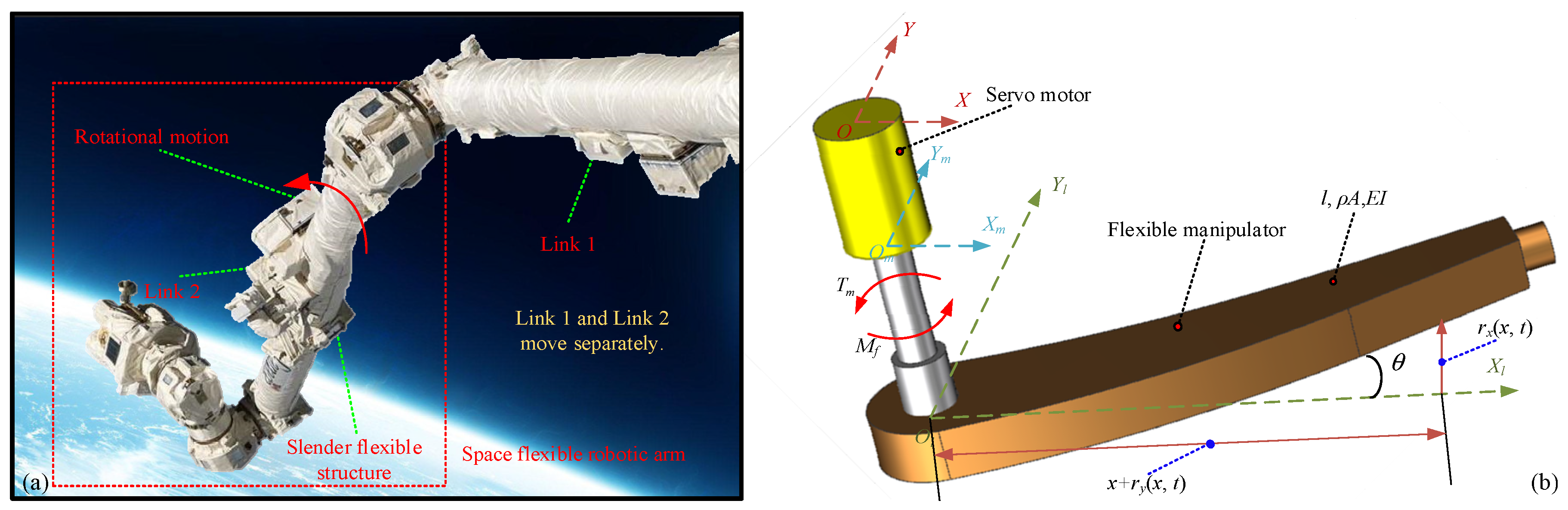
2. Modelling Dynamics for the SFRA

2.1. Friction Modeling

The accuracy of the dynamical modeling is crucial for the control law design of the research target. Therefore, we consider the effects of 2D deformation and disturbance torques on the SFRA, and model the SFRA dynamics in Section 2. Moreover, the established SFRA dynamics model is simplified and the modeling accuracy of the simplification models is discussed.

In the SFRA, there are numerous nonlinear disturbances. Usually, we consider nonlinear disturbances in the form of disturbance torques in the modelling of the dynamic of the research system. Whereas the model of disturbance torques is generally referred to as the friction model. The common friction models are the Stribeck friction model, the Dahl friction model, the LuGre friction model, the Coulomb friction model, and the Bliman-Sorine friction model. The Stribeck friction model has advantages over other friction models in terms of the accurate description of friction behavior and ease of calculation. Therefore, this paper chooses the Stribeck friction model to indicate the disturbance torque within the SFRA.

Generally, the mathematical formulation of the Stribeck friction model is:

$$M_f=F_c+\left(F_s-F_c\right)e^{-{\left(v/v_s\right)}^{\epsilon }}$$

(1)

where F_c is the coulomb friction (F_c = µ |F_n|, µ is friction coefficient, F_n is normal force); F_s is the maximum static friction; ε is an empirical constant; v_s is Stribeck speed.

The Gaussian model is adopted in this paper with ε = 2. Under this condition, the Stribeck friction model is approximately equivalently to the Lorentzian model [43], and the mathematical expression is:

$$M_f=F_c\mathrm{sgn}\left(v\right)+\left(F_s-F_c\right){\displaystyle \frac{1}{1+{\left(v/v_s\right)}^2}}$$

(2)

2.2. Dynamic Modeling

In this paper, the SFRA for space operations is studied, as reflected in Figure 1. Figure 1a is a hypothetical prototype of the space manipulator. In Figure 1a, the space robot arm is composed of slender flexible links, including link 1 and link 2. It is assumed that link 1 and link 2 move independently, so when the link 2 moves, link 1 can be considered to be relatively static. Figure 1b is the model equivalent diagram of the SFRA. It is stated that the SFRA is directly driven by the motor, and small deformation occurs during the movement. In Figure 1b, XOY is the fixed coordinate system, X_lO_lY_l, is the SFRA’s moving coordinate system, and X_mO_mY_m, is the coordinate system of motor rotation. M_f represents the equivalent disturbance; T_m represents the actuating torque. m is the mass of the SFRA; ρA is the linear density of the SFRA; l is the length of the SFRA, x is the horizontal coordinate of any point on the SFRA, EI is the flexural rigidity of the SFRA, θ is the rotation angle of the SFRA. r_x (x, t) is the transverse deformation; r_y (x, t) is the longitudinal deformation.

The deformation description of the SFRA can be represented by the beam model. Most of the beam models use the AMM to study their vibration problems. So this paper adopts the AMM to represent the transverse deformation and longitudinal deformation for the SFRA.

According to the Literature [44], the effect of higher-order modes on the accuracy of the SFRA model is small, only 1st order mode is retained in the dynamic modelling of SFRA. Therefore, the transverse deformation and longitudinal deformation of the SFRA are:

$$\{\begin{array}{l}{r}_x\left(x,t\right)={\delta }_1\left(x\right){\beta }_1\left(t\right)\\ {\delta }_1\left(x\right)=\cos \mathrm{h}\left({\alpha }_{1}x\right)-\cos \left({\alpha }_{1}x\right)+\\ {\xi }_1\left(\sin \mathrm{h}\left({\alpha }_{1}x\right)-\sin \left({\alpha }_{1}x\right)\right)\\ {\xi }_1=-{\displaystyle \frac{\sin \mathrm{h}\left({\alpha }_{1}l\right)-\sin \left({\alpha }_{1}l\right)}{\cos \mathrm{h}\left({\alpha }_{1}l\right)+\cos \left({\alpha }_{1}l\right)}}\end{array}$$

(3)

$$\{\begin{array}{l}{\displaystyle \frac{\partial r_y\left(x,t\right)}{\partial x}}=\sqrt{1-{\left({\displaystyle \frac{\partial r_x\left(x,t\right)}{\partial x}}\right)}^2}-1\approx -{\displaystyle \frac{1}{2}}{\left({\displaystyle \frac{\partial r_x\left(x,t\right)}{\partial x}}\right)}^2\\ r_y\left(x,t\right)=-{\displaystyle \frac{1}{2}}{\displaystyle {\int }_0^x{\left(\frac{\partial r_x\left(\tau ,t\right)}{\partial \tau }\right)}^2}\mathrm{d}\tau =-{\displaystyle \frac{1}{2}}{\displaystyle {\int }_0^x{\left({\beta }_1\left(t\right){\delta }_{\prime }^1\left(\tau \right)\right)}^2}\mathrm{d}\tau \end{array}$$

(4)

where ${\delta }_1\left(x\right)$ is the first-order modal function; ${\beta }_1\left(t\right)$ is the first-order modal coordinate; α₁ is the characteristic root of the first-order modal function and α₁ can be derived from solving $\cos \left({\alpha }_{1}l\right)\cos \mathrm{h}\left({\alpha }_{1}l\right)=-1$.

For simplification, the symbols defined below are all valid.

$$\begin{gathered} {\displaystyle \frac{\partial (\ast )}{\partial x}}=(\ast {)}^{\prime }, {\displaystyle \frac{\partial (\ast )}{\partial x^2}}=(\ast {)}^{″}, {\displaystyle \frac{\partial (\ast )}{\partial t}}=\stackrel{·}{(\ast )}, {\displaystyle \frac{\partial (\ast )}{\partial t^2}}=\stackrel{··}{(\ast )}; \\ {r}_x\left(x,t\right)=r_x; r_y\left(x,t\right)=r_y; {\dot{r}}_x\left(x,t\right)={\dot{r}}_x; \\ {\dot{r}}_y\left(x,t\right)={\dot{r}}_y; r_x^{″}\left(x,t\right)=r_x^{″}; \\ {\delta }_1\left(x\right)={\delta }_1; {\delta }_1^{\prime }\left(x\right)={\delta }_1^{\prime }; {\delta }_1^{\prime }\left(\tau \right)=\widehat{{\delta }_1^{\prime }}; \\ {\delta }_1^{″}\left(x\right)={\delta }_1^{″}; {\beta }_1\left(t\right)={\beta }_1; {\dot{\beta }}_1\left(t\right)={\dot{\beta }}_1; {\ddot{\beta }}_1\left(t\right)={\ddot{\beta }}_1 \end{gathered}$$

From Equations (3) and (4), the vector of displacement at any point on the SFRA is:

$$\mathit{R}=\left[\begin{array}{c}X\\ Y\end{array}\right]=A\left(\theta \right)\left[\begin{array}{c}x+r_y\\ r_x\end{array}\right]$$

(5)

where A(θ) denotes the rotational transformation matrix, which is specifically expressed as:

$$A\left(\theta \right)=\left[\begin{array}{cc}\cos \theta & -\sin \theta \\ \sin \theta & \cos \theta \end{array}\right]$$

The SFRA’s kinetic energy is:

$$\begin{array}{l}T={\displaystyle \frac{1}{2}}\rho A{\displaystyle {\int }_0^l{\dot{\mathit{R}}}^{\mathrm{T}}\dot{\mathit{R}}\mathrm{d}x}\\ ={\displaystyle \frac{1}{2}}\rho A{\displaystyle {\int }_0^l\left[\left({\left(x+r_y\right)}^2+{r_x}^2\right){\dot{\theta }}^2+\left({{\dot{r}}_x}^2+{{\dot{r}}_y}^2\right)+\left(2\left(x+r_y\right){\dot{r}}_x-2{\dot{r}}_y{r}_x\right)\dot{\theta }\right]\mathrm{d}x}\end{array}$$

(6)

The SFRA’s lightweight and slender characteristics cause it to deform elastically during motion. Thus, the potential energy of the SFRA is:

$$V={\displaystyle \frac{1}{2}}EI{\displaystyle {\int }_0^l{\left(r_x^{″}\right)}^2}\mathrm{d}x$$

(7)

According to the Lagrange principle, the equations below hold.

$$\{\begin{array}{l}{\displaystyle \frac{\mathrm{d}}{\mathrm{d}t}}\left({\displaystyle \frac{\partial T}{\partial \dot{\theta }}}\right)-{\displaystyle \frac{\partial T}{\partial \theta }}+{\displaystyle \frac{\partial V}{\partial \theta }}=T_m-M_f\\ {\displaystyle \frac{\mathrm{d}}{\mathrm{d}t}}\left({\displaystyle \frac{\partial T}{\partial {\dot{\beta }}_1\left(t\right)}}\right)-{\displaystyle \frac{\partial T}{\partial {\beta }_1\left(t\right)}}+{\displaystyle \frac{\partial V}{\partial {\beta }_1\left(t\right)}}=0\end{array}$$

(8)

The expressions for kinetic and potential energy of the SFRA can be substituted into Equation (8) to derive the dynamic equations of the SFRA, as shown in Equation (9).

$$\{\begin{array}{l}\ddot{\theta }\rho A{\displaystyle {\int }_0^l{x}^2\mathrm{d}x}+\left({\displaystyle \frac{1}{4}}\ddot{\theta }{{\beta }_1}^4+\dot{\theta }{\dot{\beta }}_1{{\beta }_1}^3\right)\rho A{\displaystyle {\int }_0^l{\left({\displaystyle {\int }_0^x{{\hat{\delta }}_1^{\prime }}^2}\mathrm{d}\tau \right)}^2\mathrm{d}x}-\\ \left(\ddot{\theta }{{\beta }_1}^2+2\dot{\theta }{\dot{\beta }}_1{\beta }_1\right)\rho A{\displaystyle {\int }_0^{l}x\left({\displaystyle {\int }_0^x{{\hat{\delta }}_1^{\prime }}^2}\mathrm{d}\tau \right)\mathrm{d}x}+\left(\ddot{\theta }{{\beta }_1}^2+2\dot{\theta }{\dot{\beta }}_1{\beta }_1\right)\rho A{\displaystyle {\int }_0^l{{\delta }_1}^2\mathrm{d}x}+\\ {\ddot{\beta }}_1\rho A{\displaystyle {\int }_0^{l}x{\delta }_1\mathrm{d}x}+{\displaystyle \frac{1}{2}}({\ddot{\beta }}_1{{\beta }_1}^2+2{{\dot{\beta }}_1}^2{\beta }_1)\rho A{\displaystyle {\int }_0^l\left({\delta }_1{\displaystyle {\int }_0^x{{\hat{\delta }}_1^{\prime }}^2}\mathrm{d}\tau \right)\mathrm{d}x}=T_m-M_f\\ \ddot{\theta }\rho A{\displaystyle {\int }_0^{l}x{\delta }_1\mathrm{d}x}+{\displaystyle \frac{1}{2}}\ddot{\theta }{{\beta }_1}^2\rho A{\displaystyle {\int }_0^l\left({\delta }_1{\displaystyle {\int }_0^x{{\hat{\delta }}_1^{\prime }}^2}\mathrm{d}\tau \right)\mathrm{d}x}+{\ddot{\beta }}_1\rho A{\displaystyle {\int }_0^l{{\delta }_1}^2\mathrm{d}x}+\\ \left({\ddot{\beta }}_1{{\beta }_1}^2+2{{\dot{\beta }}_1}^2{\beta }_1\right)\rho A{\displaystyle {\int }_0^l{\left({\displaystyle {\int }_0^x{{\hat{\delta }}_1^{\prime }}^2}\mathrm{d}\tau \right)}^2\mathrm{d}x}-{\displaystyle \frac{1}{2}}{\dot{\theta }}^2{{\beta }_1}^3\rho A{\displaystyle {\int }_0^l{\left({\displaystyle {\int }_0^x{{\hat{\delta }}_1^{\prime }}^2}\mathrm{d}\tau \right)}^2\mathrm{d}x}+\\ {\dot{\theta }}^2{\beta }_1\rho A{\displaystyle {\int }_0^{l}x\left({\displaystyle {\int }_0^x{{\hat{\delta }}_1^{\prime }}^2}\mathrm{d}\tau \right)\mathrm{d}x}-{\dot{\theta }}^2{\beta }_1\rho A{\displaystyle {\int }_0^l{{\delta }_1}^2\mathrm{d}x}+{\beta }_{1}EI{\displaystyle {\int }_0^l{{\hat{\delta }}_1^{″}}^2}\mathrm{d}x=0\end{array}$$

(9)

For writing purposes, the following symbol expressions are defined.

$$\begin{gathered} {\eta }_1=\rho A{\displaystyle {\int }_0^l{x}^2\mathrm{d}x}; {\eta }_2=\rho A{\displaystyle {\int }_0^l{\left({\displaystyle {\int }_0^x{{\hat{\delta }}_1^{\prime }}^2}\mathrm{d}\tau \right)}^2\mathrm{d}x}; \\ {\eta }_3=\rho A{\displaystyle {\int }_0^{l}x\left({\displaystyle {\int }_0^x{{\hat{\delta }}_1^{\prime }}^2}\mathrm{d}\tau \right)\mathrm{d}x}; {\eta }_4=\rho A{\displaystyle {\int }_0^l{{\delta }_1}^2\mathrm{d}x}; \\ {\eta }_5=\rho A{\displaystyle {\int }_0^{l}x{\delta }_1\mathrm{d}x}; {\eta }_6=\rho A{\displaystyle {\int }_0^l\left({\delta }_1{\displaystyle {\int }_0^x{{\hat{\delta }}_1^{\prime }}^2}\mathrm{d}\tau \right)\mathrm{d}x}; \\ {\eta }_7=EI{\displaystyle {\int }_0^l{{\delta }_1^{″}}^2}\mathrm{d}x. \end{gathered}$$

Then Equation (9) can be rewritten as

$$\{\begin{array}{l}\ddot{\theta }{\eta }_1+\left({\displaystyle \frac{1}{4}}\ddot{\theta }{{\beta }_1}^4+\dot{\theta }{\dot{\beta }}_1{{\beta }_1}^3\right){\eta }_2-\left(\ddot{\theta }{{\beta }_1}^2+2\dot{\theta }{\dot{\beta }}_1{\beta }_1\right){\eta }_3+\\ \left(\ddot{\theta }{{\beta }_1}^2+2\dot{\theta }{\dot{\beta }}_1{\beta }_1\right){\eta }_4+{\ddot{\beta }}_1{\eta }_5+{\displaystyle \frac{1}{2}}({\ddot{\beta }}_1{{\beta }_1}^2+2{{\dot{\beta }}_1}^2{\beta }_1){\eta }_6=T_m-M_f\\ \ddot{\theta }{\eta }_5+{\displaystyle \frac{1}{2}}\ddot{\theta }{{\beta }_1}^2{\eta }_6+{\ddot{\beta }}_1{\eta }_4+\left({\ddot{\beta }}_1{{\beta }_1}^2+2{{\dot{\beta }}_1}^2{\beta }_1\right){\eta }_2-\\ {\displaystyle \frac{1}{2}}{\dot{\theta }}^2{{\beta }_1}^3{\eta }_2+{\dot{\theta }}^2{\beta }_1{\eta }_3-{\dot{\theta }}^2{\beta }_1{\eta }_4+{\beta }_1{\eta }_7=0\end{array}$$

(10)

2.3. Dynamical Model Simplification

Numerous nonlinear factors are affecting the dynamical model of the SFRA, including the deformation resulting from higher-order modes, the coupling of two-dimensional deformation, and so on. Therefore the dynamics equations of the SFRA contain a large number of nonlinear terms, which make it hard to design the controller of the SFRA. In addition, the presence of nonlinear terms also makes the calculation of the SFRA dynamics model complex and difficult to solve. Therefore, the dynamics model of the SFRA needs to be simplified. Equation (10) represents the dynamic model of the SFRA, taking into account the 2D deformation, which is denoted as 2D1M. To make the dynamic equations of the SFRA simple, the longitudinal deformation or nonlinear terms can be neglected. The simplified dynamic models are to consider only the transverse deformation of the SFRA, which is denoted as 1D1M, and neglect the nonlinear terms of the SFRA, which is denoted as NNTs.

2.3.1. 1D1M Simplification Model

Only taking into account the transverse deformation of the SFRA, the vector of displacements at any point of the SFRA is:

$$\mathit{R}=\left[\begin{array}{c}X\\ Y\end{array}\right]=A\left(\theta \right)\left[\begin{array}{c}x\\ r_x\end{array}\right]$$

(11)

Thus the SFRA’s kinetic energy is:

$$T={\displaystyle \frac{1}{2}}\rho A{\displaystyle {\int }_0^l{\dot{\mathit{R}}}^{\mathrm{T}}\dot{\mathit{R}}\mathrm{d}x}={\displaystyle \frac{1}{2}}\rho A{\displaystyle {\int }_0^l\left[\left(x^2+{r_x}^2\right){\dot{\theta }}^2+{{\dot{r}}_x}^2+2x{\dot{r}}_x\dot{\theta }\right]\mathrm{d}x}$$

(12)

Since the expression for the potential energy of the SFRA is not relevant to the longitudinal deformation, the potential energy of the SFRA maintain as Equation (7). By combining Equations (7), (8) and (12), the SFRA’s dynamic equations which consider the transverse deformation can be obtained as follows.

$$\{\begin{array}{l}\ddot{\theta }{\eta }_1+\left(\ddot{\theta }{{\beta }_1}^2+2\dot{\theta }{\dot{\beta }}_1{\beta }_1\right){\eta }_4+{\ddot{\beta }}_1{\eta }_5=T_m\\ \ddot{\theta }{\eta }_5+{\ddot{\beta }}_1{\eta }_4-{\dot{\theta }}^2{\beta }_1{\eta }_4+{\beta }_1{\eta }_7=0\end{array}$$

(13)

2.3.2. NNTs Simplification Model

Equation (10) can be simplified by neglecting the nonlinear terms, and the power equation of SFRA can be rewritten as:

$$\{\begin{array}{l}\ddot{\theta }{\eta }_1+{\ddot{\beta }}_1{\eta }_5=T_m-M_f\\ \ddot{\theta }{\eta }_5+{\ddot{\beta }}_1{\eta }_4+{\beta }_1{\eta }_7=0\end{array}$$

(14)

where ω₁ is the first-order natural frequency of the SFRA.

Therefore, Equation (14) can be rewritten as:

$$\{\begin{array}{l}\ddot{\theta }{\eta }_1+{\ddot{\beta }}_1{\eta }_5=T_m-M_f\\ \ddot{\theta }{\eta }_5+{\ddot{\beta }}_1+{\beta }_1{{\omega }_1}^2=0\end{array}$$

(15)

3. Accuracy Evaluation of the Simplified Model

During the process of modelling the SFRA dynamic model, due to complexity of certain coupling terms, nonlinear terms will be generated. The nonlinear terms will increase the complexity of the simulation calculation. In this paper, the two simplified methods, 1D1M model that only considered the lateral deformation of SFRA and NNTs model that neglected the nonlinear terms, were designed. To check the efficiency of the simplified model, this paper simulates and analyzes the three simplification methods of dynamic model of 2D1M, 1D1M, and NNTs, and compares their modeling accuracy. Flexible deformation is an important parameter of the SFRA. In this section, the modeling accuracy is compared by the flexible deformation of three simplified methods. Both methods are effective in reduce the amount of computation and make the dynamic equation easier to solve.

The SFRA flexible deformation is greatly affected by length, structural mass, and flexural stiffness. This section uses the SFRA physical parameters in

Table 1. Condition parameters of the SFRA.

Condition	l (m)	M (kg)	${\dot{\mathit{\theta }}}_{\mathbf{max}}$ (rad/s)	EI (Nm2)
Length 1 (a-i)	1	3	1	160
Length 2 (a-ii)	2	3	1	160
Length 3 (a-iii)	3	3	1	160
Mass 1 (b-i)	3.5	2	1	160
Mass 2 (b-ii)	3.5	4	1	160
Mass 3 (b-iii)	3.5	6	1	160
Flexural stiffness 1 (d-i)	3.5	5	1	80
Flexural stiffness 2 (d-ii)	3.5	5	1	200
Flexural stiffness 3 (d-iii)	3.5	5	1	320

for calculation. In this paper, the single-link deductive algorithm is used to compute the flexible deformation, and the detailed calculation process of deformation can refer to the literature [45]. The flexible deformation of the SFRA under different conditions of three simplified dynamic models, 2D1M, 1D1M, and NNTs, is compared, and the deformation curve is shown in Figure 2. Figure 2a illustrates the flexible deformation curves at various lengths. Figure 2b illustrates the flexible deformation curves with various structural masses. Figure 2c is the flexible deformation curve for various flexural stiffness.

As observed in Figure 2, with the length and structural mass increasing, the amplitude of flexible deformation increases. W With the flexural stiffness increasing, the amplitude of the flexible deformation gradually diminishes. Among them, the increase in structural mass amplitude is the most obvious. This shows that the structural mass is the main factor which affects the flexible deformation of the SFRA, and also verifies the accuracy of the NNTs simplified model. Comparing the three simplified model curves, the flexible deformation curve of the NNTs model can be observed to be closer with that of the 2D1M model. The 1D1M model flexible deformation curves is very different from the two methods. This shows that considering 2D deformation can improve the accuracy of the SFRA’s dynamic model effectively. This phenomenon is more obvious under the influence of structural mass and flexural stiffness. Moreover, since the NNTs model has similar modelling accuracy to the 2D1M model. So although the nonlinear terms are integral parts in dynamic modelling of the robotic system they have little influence on the output characteristics of the system. Thus, the simplified method of neglecting the nonlinear terms to reduce the calculations is feasible.

4. Fuzzy PI Control Based on Disturbance Observer

Based on the accuracy analysis of the SFRA’s simplified dynamics models in Section 3, it is found that the NNTs have high model accuracy. Moreover, the NNTs simplified model is simple to calculate and easy to solve. Therefore, the NNTs dynamic simplified model is chosen for the controller design in Section 4.

To eliminate the effect of the disturbing torque to the SFRA output characteristics as much as possible, this paper uses a disturbance observer to observe and compensate the disturbing torque in the SFRA. In addition, the PI control method is selected in this study. The unknown disturbing torque will lead to the uncertainty of the SFRA dynamics model. In addition, the problem of model variation cannot be solved by the traditional PI control method. To remove the shortcomings of the traditional PI controller, choosing the fuzzy rules for real time adjustment of the controller parameters.

Depending on Equation (14), the transfer function in the SFRA between motor rotation speed and actuating torque can be obtained as:

$${\displaystyle \frac{{\omega }_m\left(s\right)}{T_m\left(s\right)}}={\displaystyle \frac{1}{s^2{\eta }_1-\frac{s^4{\eta }_5^2}{s^2+{\omega }_1^2}}}={\displaystyle \frac{s^2+{\omega }_1^2}{s^3\left({\eta }_1-{\eta }_5^2\right)+s{\omega }_1^2{\eta }_1}}$$

(16)

4.1. Fuzzy Adjustment of the Controller Parameters Based on Pole Configuration

In this study, the PI control method is adopted, thus the closed-loop transfer function of the SFRA is:

$$\begin{array}{ll}\hfill G_b\left(s\right)& ={\displaystyle \frac{\left(K_p+\frac{K_I}{s}\right)\left(\frac{s^2+{\omega }_1^2}{s^3\left({\eta }_1-{\eta }_5^2\right)+s{\omega }_1^2{\eta }_1}\right)}{1+\left(K_p+\frac{K_I}{s}\right)\left(\frac{s^2+{\omega }_1^2}{s^3\left({\eta }_1-{\eta }_5^2\right)+s{\omega }_1^2{\eta }_1}\right)}}\hfill \\ & ={\displaystyle \frac{K_p{s}^3+K_I{s}^2+K_p{\omega }_1^{2}s+K_I{\omega }_1^2}{\left({\eta }_1-{\eta }_5^2\right)s^4+K_p{s}^3+\left(K_I+{\omega }_1^2{\eta }_1\right)s^2+K_p{\omega }_1^{2}s+K_I{\omega }_1^2}}\hfill \end{array}$$

(17)

where K_I and K_P are the integral parameter and proportional parameter of the controller, respectively.

Referring to the pole configuration [46], the denominator polynomial in Equation (18) is written as shown in Equation (19).

$$\begin{array}{l}\left({\eta }_1-{\eta }_5^2\right)s^4+K_p{s}^3+\left(K_I+{\omega }_1^2{\eta }_1\right)s^2+K_p{\omega }_1^{2}s+K_I{\omega }_1^2\\ =s^4+{\displaystyle \frac{K_p}{{\eta }_1-{\eta }_5^2}}{s}^3+{\displaystyle \frac{\left(K_I+{\omega }_1^2{\eta }_1\right)}{{\eta }_1-{\eta }_5^2}}{s}^2+{\displaystyle \frac{K_p{\omega }_1^2}{{\eta }_1-{\eta }_5^2}}s+{\displaystyle \frac{K_I{\omega }_1^2}{{\eta }_1-{\eta }_5^2}}\\ =\left(s^2+2{\xi }_{a1}{\omega }_{a1}s+{\omega }_{a1}^2\right)\left(s^2+2{\xi }_{b1}{\omega }_{b1}s+{\omega }_{b1}^2\right)\end{array}$$

(18)

where ξ_a1 and ξ_b1 represent the damping coefficients of the poles; ω_a1 and ω_b1 represent the inherent frequency coefficients of the poles.

Based on Equation (19), Equation (20) can be derived.

$$\{\begin{array}{l}2\left({\xi }_{a1}{\omega }_{a1}+{\xi }_{b1}{\omega }_{b1}\right)={\displaystyle \frac{K_p}{{\eta }_1-{\eta }_5^2}}\\ 4{\xi }_{a1}{\xi }_{b1}{\omega }_{a1}{\omega }_{b1}+{\omega }_{a1}^2+{\omega }_{b1}^2={\displaystyle \frac{\left(K_I+{\omega }_1^2{\eta }_1\right)}{{\eta }_1-{\eta }_5^2}}\\ 2\left({\xi }_{a1}{\omega }_{a1}{\omega }_{b1}^2+{\xi }_{b1}{\omega }_{b1}{\omega }_{a1}^2\right)={\displaystyle \frac{K_p{\omega }_1^2}{{\eta }_1-{\eta }_5^2}}\\ {\omega }_{a1}^2{\omega }_{b1}^2={\displaystyle \frac{K_I{\omega }_1^2}{{\eta }_1-{\eta }_5^2}}\end{array}$$

(19)

The specific expression of K_P and K_I can be found in Equation (20).

$$\{\begin{array}{l}{K}_p=2\left({\xi }_{a1}{\omega }_{a1}+{\xi }_{b1}{\omega }_{b1}\right)\left({\eta }_1-{\eta }_5^2\right)\\ K_I={\displaystyle \frac{{\omega }_{a1}^2{\omega }_{b1}^2}{{\omega }_1^2}}\left({\eta }_1-{\eta }_5^2\right)\end{array}$$

(20)

The PI controller’s parameters change in real time depending on the fuzzy rules. The error e and the rate of the error ec are the inputs of the fuzzy controller. The values of Δk_P and Δk_I are the outputs of the fuzzy controller. Besides, the fuzzy domains of the input and output variables are set to [−6, 6]. The domain of e is set to [−0.1, 0.1]. The domain of the ec is set to [−0.2, 0.2]. The domains of the actual controller output are set to [−0.6, 0.6] [9]. The fuzzy set of the input and output is set to six, as shown in Equation (22).

$$e,ec,\Delta k_P,\Delta k_I=\left\{\begin{array}{ccccccc}\mathrm{NB}& \mathrm{NM}& \mathrm{NS}& \mathrm{ZO}& \mathrm{PS}& \mathrm{PM}& \mathrm{PB}\end{array}\right\}$$

(21)

where N is negative; B is large; M is moderate; S is small; P is positive; ZO is 0.

The fuzzy rules table can be shown in the literature [46]. In this paper, we use the triangular membership function as the input and output membership function. The mathematical expression of the triangular membership function is:

$$f\left(x,a,b,c\right)=\{\begin{array}{c}0 x\le a\\ {\displaystyle \frac{x-a}{b-a}} a\le x\le b\\ {\displaystyle \frac{c-x}{c-b}} b\le x\le c\\ 0 x\ge c\end{array}$$

(22)

where a, b, and c denote the parameters.

Thus, the fuzzy inference relationship can be gotten, as presented in Figure 3.

$$\{\begin{array}{l}{K}_P=K_{P0}+k_P\Delta k_P\\ K_I=K_{I0}+k_I\Delta k_I\end{array}$$

(23)

where K_P0 and K_I0 are the initial parameters of the controller; k_P and k_I are the scale factors for the controller parameters; K_P and K_I denote the controller parameters after fuzzy rules adjustment.

4.2. Design of Disturbance Observer Based on the Nominal Model

In this paper, the disturbance observer is used to observe and compensate for the disturbance torque in the SFRA. The design of the disturbance observer focuses on the establishment of the nominal transfer function and the design of the low pass filter. The speed control block diagram of the SFRA based on the disturbance observer is given in Figure 4. In Figure 4, ω_m ^∗ denotes the rated speed; C(s) denotes the PI controller; Q(s) denotes the low pass filter; M_f denotes the equivalent disturbance; $\hat{d}$ denotes the observing value of M_f; ξ denotes the measurement noise.

According to Equation (17), the transfer function of the controlled plant can be written as:

$$\{\begin{array}{l}{G}_p\left(s\right)={\displaystyle \frac{{\omega }_m\left(s\right)}{T_m\left(s\right)}}={\displaystyle \frac{s^2+M_3}{M_1{s}^3+M_{2}s}}\\ M_1={\eta }_1-{\eta }_5^2\\ M_2={\omega }_1^2{\eta }_1\\ M_3={\omega }_1^2\end{array}$$

(24)

where G_p(s) represents the actual model.

Then, the transfer function of the nominal model can be obtained as:

$$\{\begin{array}{l}{G}_n\left(s\right)={\displaystyle \frac{{\hat{\omega }}_m\left(s\right)}{{\hat{T}}_m\left(s\right)}}={\displaystyle \frac{s^2+{\hat{M}}_3}{{\hat{M}}_1{s}^3+{\hat{M}}_{2}s}}\\ {\hat{M}}_1={\hat{\eta }}_1-{\hat{\eta }}_5^2\\ {\hat{M}}_2={\hat{\omega }}_1^2{\hat{\eta }}_1\\ {\hat{M}}_3={\hat{\omega }}_1^2\end{array}$$

(25)

where G_n(s) represents the nominal model; ${\hat{\eta }}_1$, ${\hat{\eta }}_5$ and ${\hat{\omega }}_1$ represent the estimated value of ${\eta }_1$, ${\eta }_5$ and ${\omega }_1$.

It is assumed that the uncertain performance of the SFRA caused by the disturbance torque can be expressed by product perturbation. The relationship between the nominal model and the actual model can be gotten as follows.

$${\displaystyle \frac{G_p\left(s\right)}{G_n\left(s\right)}}=1+\Delta \left(s\right)$$

(26)

where $\Delta \left(s\right)$ represents the variation.

The complementary sensitivity function of the closed loop system could be obtained as [47,48]:

$$\{\begin{array}{l}T\left(s\right)={\displaystyle \frac{C\left(s\right)G_n\left(s\right)+Q\left(s\right)}{1+C\left(s\right)G_n\left(s\right)}}={\displaystyle \frac{C\left(s\right)G_n\left(s\right)+T_{DOB}\left(s\right)}{1+C\left(s\right)G_n\left(s\right)}}\\ Q\left(s\right)=T_{DOB}\left(s\right)\end{array}$$

(27)

where T_DOB(s) represents the complementary sensitivity function of the disturbance observer inner loop; C(s) represents the PI controller.

According to the literature [49], the sufficient and necessary conditions for the robust stability of the system can be obtained as:

$${\Vert \Delta \left(s\right)T_{DOB}\left(s\right)\Vert }_{\infty }={\Vert \Delta \left(s\right)Q\left(s\right)\Vert }_{\infty }\le 1$$

(28)

By Equation (29), the system is guaranteed to be stable as long as the low-pass filter satisfies Equation (30).

$${\Vert Q\left(s\right)\Vert }_{\infty }\le {\displaystyle \frac{1}{{\Vert \Delta \left(s\right)\Vert }_{\infty }}}={\displaystyle \frac{1}{{\Vert \frac{G_p\left(s\right)-G_n\left(s\right)}{G_n\left(s\right)}\Vert }_{\infty }}}$$

(29)

The low-pass filter is designed as Equation (31). By adjusting the coefficients to satisfy Equation (30), in which case the system is stable.

$$Q\left(s\right)={\displaystyle \frac{\alpha \beta \gamma }{\left(s+\alpha \right)\left(s+\beta \right)\left(s+\gamma \right)}}$$

(30)

where α, β, γ represent the parameters of the low-pass filter to be designed.

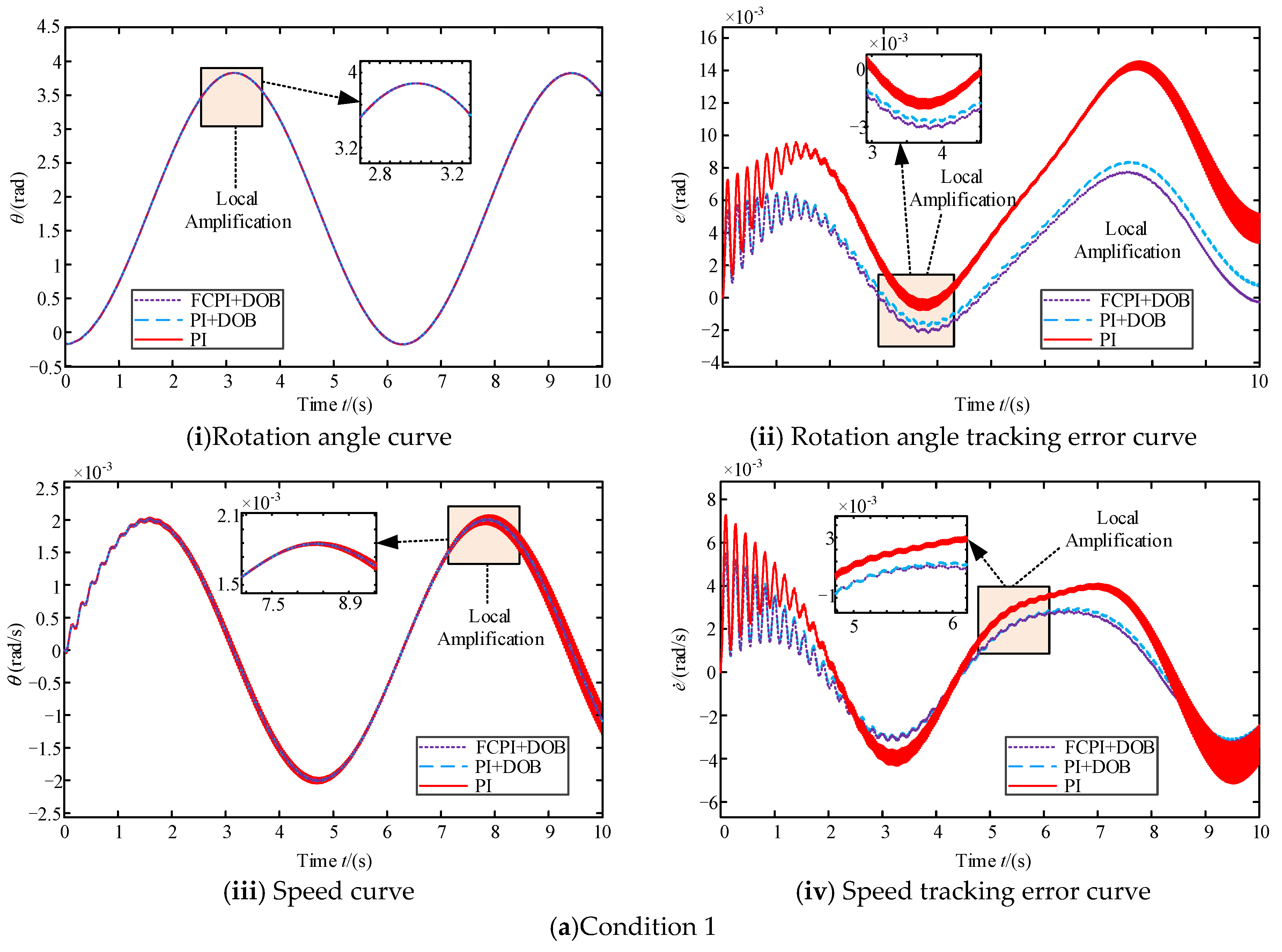
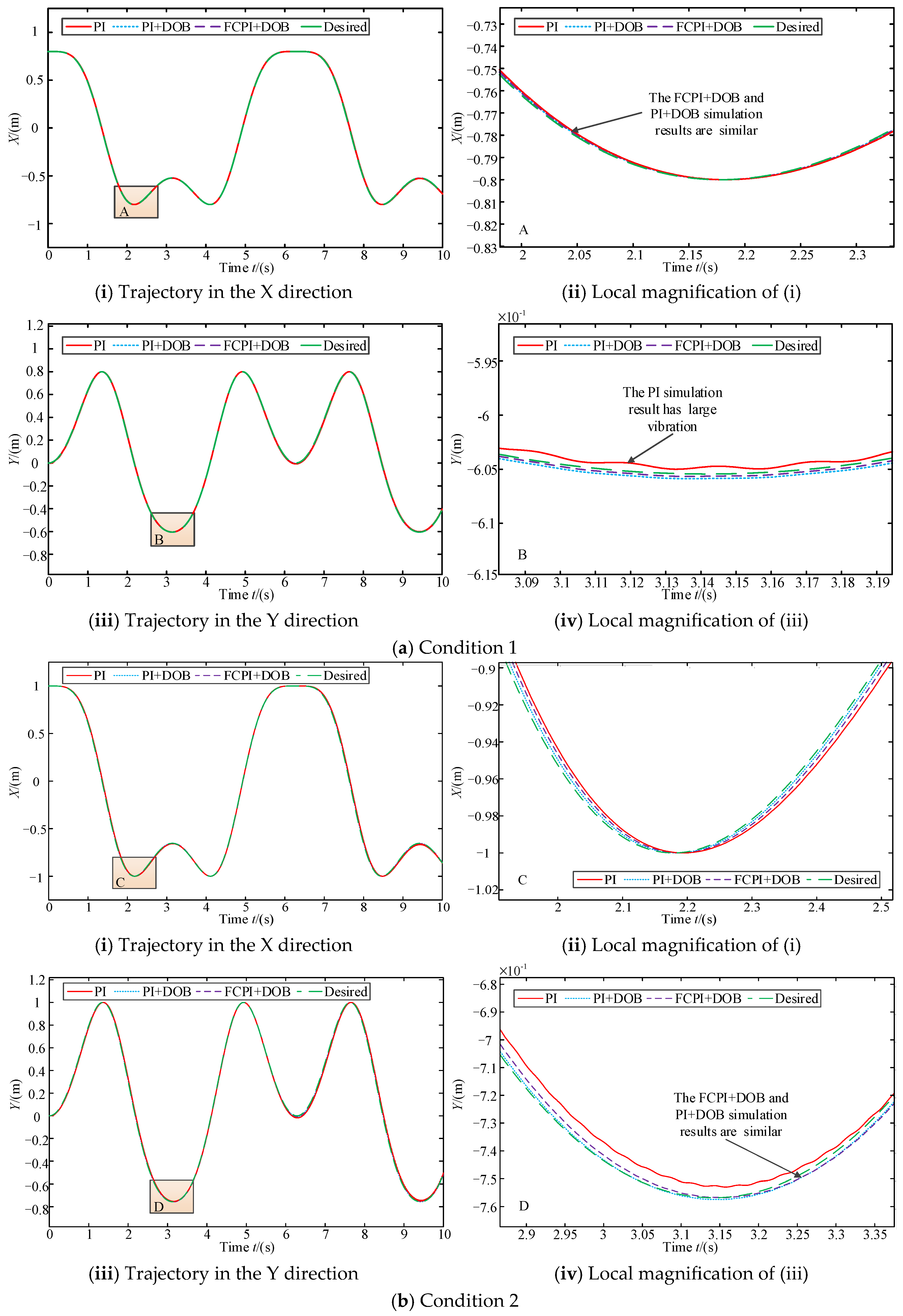
5. Simulation and Physical Prototype Control Experiments on Ground

The SFRA is subject to great external disturbance when performing tasks in space, and the traditional PI control strategy is less resistant to external disturbance. This will directly impact the SFRA control accuracy. In order to resolve this problem, this paper proposes the combined control strategy (FCPI + DOB). The strategy compensates the uncertainty through fuzzy rules, and applies the DOB control to compensate external interference to enhance the control accuracy. To verify the FCPI + DOB strategy effectiveness, it was performed with simulation analysis and ground physics control experiments. In the simulation analysis, the SFRA parameters in

Table 2. Parameters of the SFRA in Simulation.

Parameters	Condition 1	Condition 2
Length l/m	0.8	1
Mass m/kg	0.8	1.1
Flexural rigidity EI/Nm2	400	400
Coulomb friction torque Fc/Nm	0.28	0.28
Static friction torque Fs/Nm	0.34	0.34
Low-pass filter parameters α	0.1	0.1
Low-pass filter parameters β	0.1	0.1
Low-pass filter parameters γ	0.1	0.1
Controller parameters KP	20	20
Controller parameters KI	5	5

are used to compare the rotation angle, speed, deformation and trajectory of the SFRA with different control strategies. The efficiency of the FCPI + DOB strategy proposed is verified in this paper. The effectiveness of the FCPI + DOB strategy is verified through contrasting the experimental results of ground physical prototype control and simulation analysis.

5.1. Simulation Analysis

To verify that the FCPI + DOB strategy can enhance the control accuracy effectively, this section selects the output characteristics of SFRA’s rotation angle and speed, tracking error of rotation angle and speed, flexible deformation, and trajectory for comparison. In the simulation, use a sine function as the input. Three strategies of FCPI + DOB, PI + DOB, and PI are chosen to be simulated and analysed under two different conditions. The simulation results are shown below.

According to Figure 5, the three strategies have better tracking effects under condition 1. With the increase in length and quality, the speed-tracking effect of the PI strategy decreases significantly. In order to study the rotation angle and speed tracking error with the three control strategies, this section gives the tracking error curve. According to the figure, the error curves of the FCPI + DOB and the PI + DOB are similar, and the tracking error is smaller than that of the PI strategy under condition 1. This indicates that the DOB strategy can effectively compensate for external interference. As the length and quality increase, the tracking errors increase gradually for the three strategies. Nevertheless, the tracking error of the FCPI + DOB strategy does not increase significantly. This verifies that the fuzzy rules can effectively compensate the uncertainty and enhance the control accuracy. It is also proved that the FCPI + DOB strategy can effectively reduce control error.

To investigate the effect of different control strategies on the flexible deformation of the SFRA, the simulation analysis is carried out, and the results are shown in Figure 6.

According to Figure 6, the FCPI + DOB strategy and the PI + DOB strategy can obtain smaller deformation amplitude than the PI strategy under any conditions. Among them, the FCPI + DOB strategy amplitude is the smallest. This verifies that the DOB strategy can effectively compensate for external interference and obtain higher control accuracy. As the length and mass of the SFRA increase, the deformation amplitude increases gradually for the three control strategies. Nevertheless, the FCPI + DOB strategy deformation amplitude does not increase significantly. This indicates that the control strategy using fuzzy rules to compensate for uncertainties can improve the control accuracy effectively.

In order to study the influence of the FCPI + DOB strategy on the accuracy of the SFRA tracking trajectory, this paper analyzes the trajectory of the end effector under different control strategies, as indicated in Figure 7.

Based on shown in Figure 7, the PI + DOB strategy is close to the FCPI + DOB strategy in the X and Y directions. Among them, the FCPI + DOB strategy is closer to the desired trajectory. This shows that fuzzy rules can compensate for uncertainties and improve control accuracy. The PI strategy tracking effect is worse than that of the other two control strategies and has a large disturbance. This shows that the DOB strategy can effectively compensate for external interference and achieve greater control accuracy. As the length and mass of the SFRA increase, the trajectory amplitude in the X direction and Y direction increases, and the PI + DOB strategy and FCPI + DOB strategy still have a good tracking effect.

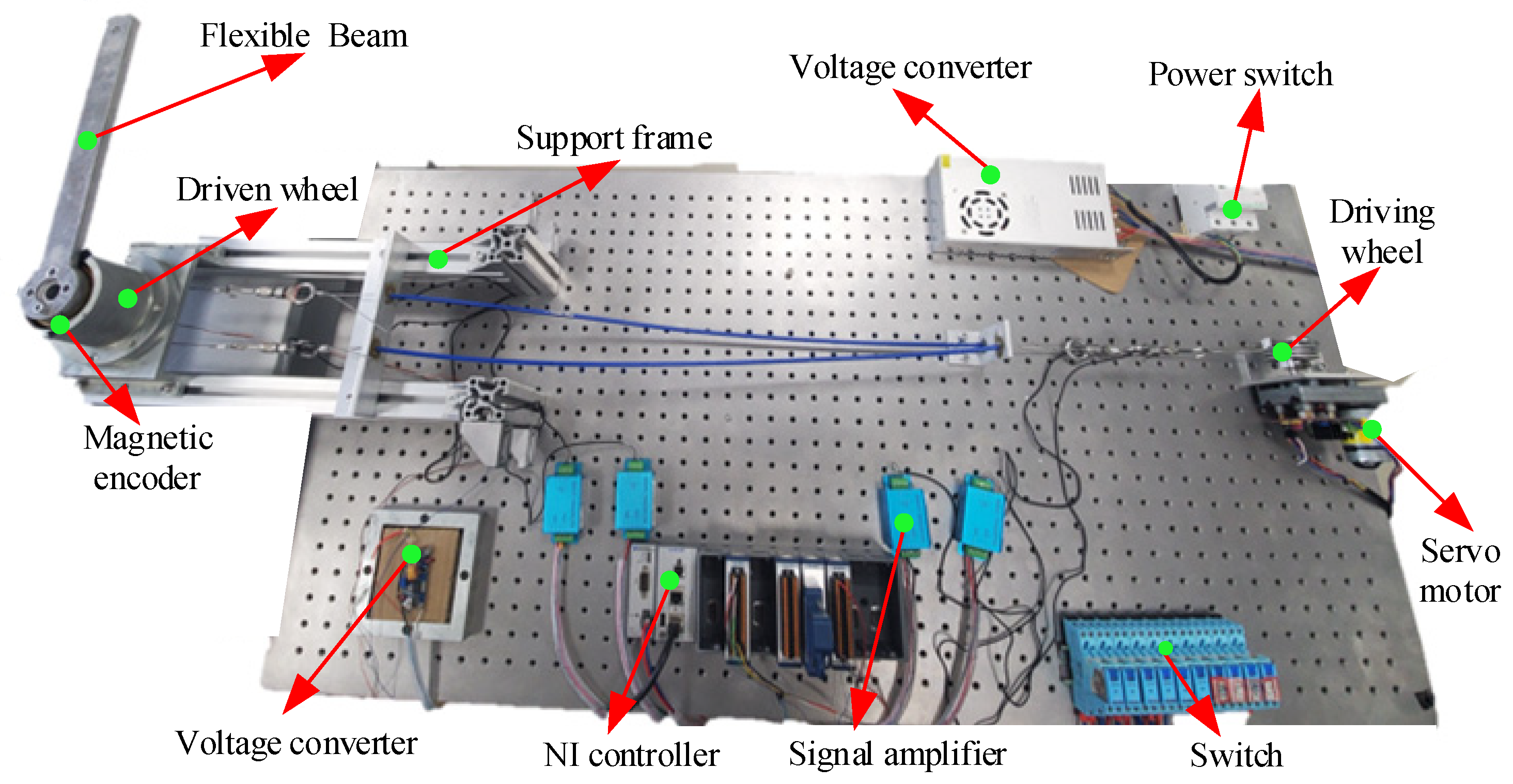
5.2. Ground Physical Prototype Control Experiment

In order to validate the efficiency of the FCPI + DOB control strategy proposed in this paper, a ground SFRA control simulation experiment platform is constructed. In order to simulate the environment in space to offset the influence of gravity, the experimental platform needs to rotate the flexible beam horizontally. As illustrated in Figure 8, the experimental platform composed of a servo motor, drive wheel, flexible beam, calculation module, data acquisition module, motor drive module, and so on. The calculation module is accountable for identifying the control program and inputting the control signal to the motor drive module. The motor drive module, through the voltage control servo motor, transmits the control torque to the drive wheel, which can realize the rotation of the flexible beam. The data acquisition module collects the SFRA rotation angle data in real-time and enters the control system.

To study the control effect of the FCPI + DOB strategy, the experimental platform compares three control strategies of FCPI + DOB strategy, PI + DOB strategy, and PI strategy by simulating different SFRA length conditions. The SFRA parameters are shown in

Table 3. Parameters of the SFRA in ground physical prototype.

Parameters	Condition 1	Condition 2	Condition 3
Length l/m	3	3.5	4
Mass m/kg	2	2	2
Flexural rigidity EI/Nm2	50	50	50
Low-pass filter parameters α	0.1	0.1	0.1
Low-pass filter parameters β	0.1	0.1	0.1
Low-pass filter parameters γ	0.1	0.1	0.1
Controller parameters KP	10	10	10
Controller parameters KI	5	5	5

. The sine function is used as the input signal of the SFRA. The experimental results under different control strategies can be acquired, as indicated in Figure 9.

As can be seen on Figure 9, all three control strategies have better tracking effects. The tracking error amplitude of the FCPI + DOB strategy is the smallest. The PI + DOB is the second, and the PI strategy tracking error amplitude is the largest. As SFRA length increases, the angle error increases slightly, and the tracking error amplitude of the FCPI + DOB strategy is still the smallest. This is because the fuzzy rules can effectively compensate for the uncertainties, and it is also verified that the FCPI + DOB control strategy can enhance the control accuracy.

This section quantifies the performance of different control strategies to explain the experimental results of different control strategies. Three evaluation indexes of absolute error mean error variance and standard deviation of error are compared. The experimental parameters are shown in

Table 4. Evaluation index of error.

	Control Strategy	Means of Absolute Error	Variance of Error	Standard Deviation of Error
Condition 1	PI	0.1587	0.0221	0.149
	PI + DOB	0.1406	0.0145	0.121
	FCPI + DOB	0.1253	0.0133	0.115
Condition 2	PI	0.1626	0.0232	0.152
	PI + DOB	0.1497	0.0195	0.139
	FCPI + DOB	0.1428	0.0152	0.123
Condition 2	PI	0.1706	0.0424	0.206
	PI + DOB	0.1643	0.0308	0.175
	FCPI + DOB	0.1462	0.0267	0.166

.

From Table 4, it can be seen that the three evaluation indexes obtained by the FCPI + DOB strategy are the smallest under the three conditions. Compared to the PI strategy, the mean absolute error of the FCPI + DOB strategy is reduced by 16.47%, the error variance is reduced by 37.05% and the standard deviation is reduced by 20.36%. This shows that the FCPI + DOB strategy has a better control effect.

Through simulation experiments and prototype control experiments, this paper proves the superiority of the FCPI + DOB strategy. Compared with the PI strategy, fuzzy rules can effectively compensate for uncertainties and improve control accuracy. The fuzzy rule control compensation strategy can make the SFRA get a better control effect.

6. Discussions

6.1. Comparison of Dynamic Modeling Methods

Accurate dynamic model is an indispensable step for high-precision control. It is important to use appropriate modeling methods to establish a dynamic model. At present, there are two common modeling methods for flexible manipulators, namely AMM and FEM. AMM uses a set of assumptions that satisfy the boundary conditions to discretize the displacement of the flexible continuum, and usually derives a model with less degrees of freedom and similar accuracy [50]. AMM is suitable for the structure of regular vibration modes, has better approximation results, high computational efficiency and is easy to implement [51]. However, it has always been a challenge for the AMM to find a series of mode functions that meet the geometrical constraint conditions for each component FEM is a computational method that can analyze the dynamics of structures with complex geometry, material distribution and boundary conditions and has high modeling accuracy [52]. However, the accuracy of the FEM depends on the size of the finite element (or mesh) used in the analysis, because the displacement field in the finite element is usually represented by simple polynomial functions that are independent of the vibration frequency. A disadvantage of FEM is that very fine mesh division is required to improve the accuracy of the solution, which will lead to a significant increase in computational costs [53]. High computational cost is not conducive to real-time control. And the dynamic model established by FEM is strongly nonlinear and strongly coupled, which is not conducive to the design of the controller. The SFRA studied in this paper is a regular shaped object and the vibration suppression of SFRA is carried out in this paper by using a control strategy that combined fuzzy adjustment PI and DOB. Therefore, in this paper, AMM is used to model the dynamics of the SFRA.

6.2. DOB Robust Stability

In this study, the DOB is mainly used to control the external disturbance of the SFRA. Parameter perturbation of the controlled object, external disturbance and parameter change of the controller will affect the DOB robust stability. The robust stability of the DOB under parametric perturbation has been thoroughly discussed by Shang et al. [48] and Jun et al. [49]. According to the above literature, the parameters of the low-pass filter can meet the robust stability criteria formed by the above functions by setting the complementary sensitivity function, the upper limit function and the equivalent weight function, so as to ensure the robust stability of the system under parameter perturbation. However, the focus of this paper is to discuss the application of the DOB, rather than the robust stability analysis of the DOB. For the analysis of the robust stability of DOB, the reader can refer to the above literature.

7. Conclusions

In this paper, the SFRA is selected as the object of research, and the dynamic model is established using the AMM. In the process of building the SFRA dynamic model, the 2D deformation and external disturbance are considered. Compared with the traditional dynamic modeling method considering only transverse deformation, the dynamic modeling method considering the 2D deformation proposed in this paper has higher model accuracy. In order to simplify the kinetic model of SFRA and improve the computational efficiency, this paper proposes a simplification method that ignores the nonlinear terms. This method maintains a high modelling accuracy while reducing model complexity.

An advanced control strategy that combines the fuzzy adjustment PI controller and the DOB) is designed in this paper. This combined strategy not only adjusts the controller parameters in real time to reduce the tracking error, but also mitigates the negative impact of external perturbations on the system with the DOB. Compared with the traditional PI control method, the control strategy proposed in this study shows a significant advantage in reducing the SFRA tracking error. The experimental results show that the strategy is capable of reducing the tracking error of SFRA by 16.47%.

The validity of the control strategy proposed in this paper is demonstrated through the verification of simulation and physical prototype experiments. These findings not only provide new solutions for the precise control of SFRA, but also contribute valuable insights to the field of modelling and controlling the dynamics of flexible manipulators.

References

1. Moghaddam, B.M.; Chhabra, R. On the guidance, navigation and control of in-orbit space robotic missions: A survey and prospective vision. Acta Astronaut. 2021, 184, 70–100. [Google Scholar] [CrossRef]
2. Li, Y.M.; Tong, S.C.; Li, T.S. Adaptive fuzzy output feedback control for a single-link flexible robot manipulator driven DC motor via backstepping, Nonlinear Anal. Real World Appl. 2012, 14, 483–494. [Google Scholar] [CrossRef]
3. Li, W.J.; Cheng, D.Y.; Liu, X.G.; Wang, Y.B.; Shi, W.H.; Tang, Z.X.; Gao, F.; Zeng, F.M.; Chai, H.Y.; Luo, W.B.; et al. On-orbit service (OOS) of spacecraft: A review of engineering developments. Prog. Aerosp. Sci. 2019, 108, 32–120. [Google Scholar] [CrossRef]
4. Peng, J.Q.; Xu, W.F.; Liu, T.L.; Yuan, H.; Liang, B. End-effector pose and arm-shape synchronous planning methods of a hyper-redundant manipulator for spacecraft repairing. Mech. Mach. Theory 2021, 155, 104062. [Google Scholar] [CrossRef]
5. Yang, S.J.; Zhang, Y.L.; Wen, H.; Jin, D.P. Coordinated control of dual-arm robot on space structure for capturing space targets. Adv. Space Res. 2023, 71, 2437–2448. [Google Scholar] [CrossRef]
6. Gasbarri, P.; Pisculli, A. Dynamic/control interactions between flexible orbiting space-robot during grasping, docking and post-docking manoeuvres. Acta Astronaut. 2015, 110, 225–238. [Google Scholar] [CrossRef]
7. Sabatini, M.; Gasbarri, P.; Monti, R.; Palmerini, G.B. Vibration control of a flexible space manipulator during on orbit operations. Acta Astronaut. 2012, 73, 109–121. [Google Scholar] [CrossRef]
8. Mehrjooee, O.; Dehkordi, S.F.; Korayem, M.H. Dynamic modeling and extended bifurcation analysis of flexible-link manipulator. Mech. Based Des. Struct. Mach. 2019, 48, 87–110. [Google Scholar] [CrossRef]
9. Chu, A.M.; Nguyen, C.D.; Duong, X.B.; Nguyen, A.V.; Nguyen, T.A.; Le, C.H.; Packianather, M. A novel mathematical approach for finite element formulation of flexible robot dynamics. Mech. Based Des. Struct. March. 2020, 50, 3747–3767. [Google Scholar] [CrossRef]
10. Du, H.; Lim, M.K.; Liew, K.M. A nonlinear finite element model for dynamics of flexible manipulators. Mech. Mach. Theory 1996, 31, 1109–1119. [Google Scholar] [CrossRef]
11. Hewit, J.R.; Morris, J.R.; Sato, K.; Ackermann, F. Active force control of a flexible manipulator by distal feedback. Mech. Mach. Theory 1997, 32, 583–596. [Google Scholar] [CrossRef]
12. Xiao, W.; Hu, D.A.; Yang, G.; Jiang, C. Modeling and analysis of soft robotic surfaces actuated by pneumatic network bending actuators. Smart Mater. Struct. 2022, 31, 055001. [Google Scholar] [CrossRef]
13. Zhang, X.S.; Zhang, D.G.; Chen, S.J.; Hong, J.Z. Modal characteristics of a rotating flexible beam with a concentrated mass based on the absolute nodal coordinate formulation. Nonlinear Dyn. 2017, 88, 61–77. [Google Scholar] [CrossRef]
14. Kumar, P.; Pratiher, B. Influences of generic payload and constraint force on modal analysis and dynamic responses of flexible manipulator. Mech. Based Des. Struct. Mach. 2020, 50, 1968–1986. [Google Scholar] [CrossRef]
15. Qiu, Z.C.; Li, C.; Zhang, X.M. Experimental study on active vibration control for a kind of two-link flexible manipulator. Mech. Syst. Signal Process. 2018, 118, 623–644. [Google Scholar] [CrossRef]
16. Mukherjee, S.; Roy, H. Modeling of flexible damped coupling and its influence on rotor dynamics. Mech. Based Des. Struct. Mach. 2023, 52, 1377–1398. [Google Scholar] [CrossRef]
17. Kumar, P.; Pratiher, B. Nonlinear dynamic analysis of a multi-link manipulator with flexible links-joints mounted on a mobile platform. Adv. Space Res. 2023, 71, 2095–2127. [Google Scholar] [CrossRef]
18. Korayem, M.H.; Shafei, A.; Absalan, M.; Kadkhodaei, F.B.; Azimi, A. Kinematic and dynamic modeling of viscoelastic robotic manipulators using Timoshenko beam theory: Theory and experiment. Int. J. Adv. Manuf. Technol. 2014, 71, 1005–1018. [Google Scholar] [CrossRef]
19. Mahto, S. Shape optimization of revolute-jointed single link flexible manipulator for vibration suppression. Mech. Mach. Theory 2014, 75, 150–160. [Google Scholar] [CrossRef]
20. Guo, F.; Cheng, G.; Pang, Y.S. Explicit dynamic modeling with joint friction and coupling analysis of a 5-dof hybrid polishing robot. Mech. Mach. Theory 2022, 167, 104509. [Google Scholar] [CrossRef]
21. He, J.; Zheng, H.C.; Gao, F.; Zhang, H.B. Dynamics and control of a 7-DOF hybrid manipulator for capturing a non-cooperative target in space. Mech. Mach. Theory 2019, 140, 83–103. [Google Scholar] [CrossRef]
22. Cui, L.L.; Wang, H.S.; Chen, W.D. Trajectory Planning of a Spatial Flexible Manipulator for Vibration Suppression. Rob. Auton. Syst. 2019, 123, 103316. [Google Scholar] [CrossRef]
23. Kim, H.K.; Choi, S.B.; Thompson, B.S. Compliant control of a two-link flexible manipulator featuring piezoelectric actuators. Mech. Mach. Theory 2001, 36, 411–424. [Google Scholar] [CrossRef]
24. Malgaca, L.; Yavuz, A.; Akda, M.; Karagülle, H. Residual vibration control of a single-link flexible curved manipulator. Simul. Modell. Pract. Theory 2016, 67, 155–170. [Google Scholar] [CrossRef]
25. Han, D.; Dong, G.Q.; Huang, P.F.; Ma, Z.Q. Capture and detumbling control for active debris removal by a dual-arm space robot. Chin. J. Aeronaut. 2022, 35, 342–353. [Google Scholar] [CrossRef]
26. Ahmadizadeh, M.; Shafei, A.M.; Fooladi, M. Dynamic modeling of closed-chain robotic manipulators in the presence of frictional dynamic forces: A planar case. Mech. Based Des. Struct. Mach. 2021, 51, 4347–4367. [Google Scholar] [CrossRef]
27. Huang, J.B.; Xie, Z.W.; Jin, M.H.; Jiang, Z.N.; Liu, H. Adaptive impedance-controlled manipulator based on collision detection. Chin. J. Aeronaut. 2009, 22, 105–112. [Google Scholar] [CrossRef]
28. Feyzollahzadeh, M.; Bamdad, M. Efficient technique in computational dynamic modeling of a flexible manipulator with large deformation. J. Vib. Control 2023, 29, 2227–2241. [Google Scholar] [CrossRef]
29. Bamdad, M.; Feyzollahzadeh, M. Computational efficient discrete time transfer matrix method for large deformation analysis of flexible manipulators. Mech. Based Des. Struct. Mach. 2020, 50, 4274–4296. [Google Scholar] [CrossRef]
30. Liu, X.F.; Li, H.Q.; Chen, Y.J.; Cai, G.P. Dynamics and control of space robot considering joint friction. Acta Astronaut. 2015, 111, 1–18. [Google Scholar] [CrossRef]
31. Zhai, G.; Zheng, H.M.; Zhang, B. Observer-based control for the platform of a tethered space robot. Chin. J. Aeronaut. 2018, 31, 1786–1796. [Google Scholar] [CrossRef]
32. Ibrahim, K.; Sharkawy, A.B. A hybrid PID control scheme for flexible joint manipulators and a comparison with sliding mode control. Ain Shams Eng. J. 2019, 9, 3451–3457. [Google Scholar] [CrossRef]
33. Lu, K.; Han, S.; Yang, J.; Yu, H. Inverse Optimal Adaptive Tracking Control of Robotic Manipulators Driven by Compliant Actuators. IEEE Trans. Ind. Electron. 2023, 71, 6139–6149. [Google Scholar] [CrossRef]
34. Zhang, S.; Schmidt, R.; Qin, X.S. Active vibration control of piezoelectric bonded smart structures using PID algorithm. Chin. J. Aeronaut. 2015, 28, 305–313. [Google Scholar] [CrossRef]
35. Ranjan, R.; Dwivedy, S.K. Dynamic analysis and control of a string-stiffened single-link flexible manipulator with flexible joint. Mech. Based Des. Struct. Mach. 2022, 51, 6329–6359. [Google Scholar] [CrossRef]
36. Ravandi, A.K.; Khanmirza, E.; Daneshjou, K. Hybrid force/position control of robotic arms manipulating in uncertain environments based on adaptive fuzzy sliding mode control. Appl. Soft Comput. 2018, 70, 864–874. [Google Scholar] [CrossRef]
37. Chen, J.H.; Huang, T.C. Applying neural networks to on-line updated pid controllers for nonlinear process control. J. Process Control 2004, 14, 211–230. [Google Scholar] [CrossRef]
38. Wen, S.H.; Zheng, W.; Jia, S.D.; Ji, Z.X.; Hao, P.C.; Lam, H.K. Unactuated Force Control of 5-DOF Parallel Robot Based on Fuzzy PI. Int. J. Control Autom. Syst. 2020, 18, 1629–1641. [Google Scholar] [CrossRef]
39. Aghayan, Z.S.; Alfi, A.; Lopes, A.M. Disturbance observer-based delayed robust feedback control design for a class of uncertain variable fractional-order systems: Order-dependent and delay-dependent stability. ISA Trans. 2023, 138, 20–36. [Google Scholar] [CrossRef]
40. Jiang, T.T.; Liu, J.K.; He, W. Boundary control for a flexible manipulator based on infinite dimensional disturbance observer. J. Sound. Vib. 2015, 348, 1–14. [Google Scholar] [CrossRef]
41. Shang, D.Y.; Li, X.P.; Yin, M.; Li, F.J. Speed control strategy of dual flexible servo system considering time-varying parameters for a flexible manipulator with an axially translating arm. Asian J. Control 2023, 25, 61975. [Google Scholar] [CrossRef]
42. Yin, H.B.; Kobayashi, Y.; Hoshino, Y.; Emaru, T. Modeling and vibration analysis of flexible robotic arm under fast motion in consideration of nonlinearity. J. Syst. Des. Dyn. 2011, 5, 909–924. [Google Scholar] [CrossRef]
43. Hess, D.P.; Soom, A. Friction at a lubricated line contact operating at oscillating sliding velocities. J. Tribol. 1990, 112, 147–152. [Google Scholar] [CrossRef]
44. Shang, D.Y.; Li, X.P.; Yin, M.; Li, F.J. Dynamic modeling and fuzzy adaptive control strategy for space flexible robotic arm considering joint flexibility based on improved sliding mode controller. Adv. Space Res. 2022, 70, 3520–3539. [Google Scholar] [CrossRef]
45. Shang, D.Y.; Li, X.P.; Yin, M.; Li, F.J. Dynamic modeling and fuzzy compensation sliding mode control for flexible manipulator servo system. Appl. Math. Modell. 2022, 107, 530–556. [Google Scholar] [CrossRef]
46. Feliu, V.; Pereira, E.; Diaz, I.M. Passivity-based control of single-link flexible manipulators using a linear strain feedback. Mech. Mach. Theory 2013, 71, 191–208. [Google Scholar] [CrossRef]
47. Shang, D.Y.; Li, X.P.; Yin, M.; Li, F.J.; Wen, B.C. Rotation Angle Control Strategy for Telescopic Flexible Manipulator Based on a Combination of Fuzzy Adjustment and RBF Neural Network. Chin. J. Mech. Eng. 2022, 35, 53. [Google Scholar] [CrossRef]
48. Shang, D.Y.; Li, X.P.; Yin, M.; Li, F.J. Speed control method for dual-flexible manipulator with a telescopic arm considering bearing friction based on adaptive PI controller with DOB. Alex. Eng. J. 2022, 61, 4741–4756. [Google Scholar] [CrossRef]
49. Yun, J.N.; Su, J.B.; Kim, Y.I.; Kim, Y.C. Robust Disturbance Observer for Two-Inertia System. IEEE Trans. Ind. Electron. 2013, 60, 2700–2710. [Google Scholar] [CrossRef]
50. Sun, C.; Gao, H.; He, W.; Yu, Y. Fuzzy Neural Network Control of a Flexible Robotic Manipulator Using Assumed Mode Method. IEEE Trans. Neural Netw. Learn. Syst. 2018, 29, 5214–5227. [Google Scholar] [CrossRef]
51. Yang, X.; Liu, M.; Zhang, W.; Melnik, R.V. Invariant and energy analysis of an axially retracting beam. Chin. J. Aeronaut. 2016, 29, 952–961. [Google Scholar] [CrossRef]
52. Chen, Y.-P.; Hsu, H.-T. Regulation and Vibration Control of an FEM-Based Single- Link Flexible Arm Using Sliding-Mode Theory. J. Vib. Control 2001, 7, 741–752. [Google Scholar] [CrossRef]
53. Alandoli, E.A.; Lee, T.S.; Lin, Y.J.; Vijayakumar, V. Dynamic Model and Intelligent Optimal Controller of Flexible Link Manipulator System with Payload Uncertainty. Arab. J. Sci. Eng. 2021, 46, 7423–7433. [Google Scholar] [CrossRef]
Figure 1. The SFRA schematic view; (a) Hypothetical prototype of the SFRA; (b) Equivalent physical model of the SFRA.
Mathematics 12 02513 g001
Figure 2. Flexible deformation for different simplified dynamic models.
Mathematics 12 02513 g002aMathematics 12 02513 g002b
Figure 3. Fuzzy inference relationship.
Mathematics 12 02513 g003
Figure 4. Speed control block diagram of the SFRA.
Mathematics 12 02513 g004
Figure 5. Rotation simulation results of the SFRA with different strategies.
Mathematics 12 02513 g005aMathematics 12 02513 g005b
Figure 6. Simulation results of the SFRA deformation.
Mathematics 12 02513 g006
Figure 7. Trajectory simulation results of the end effector.
Mathematics 12 02513 g007
Figure 8. Ground physical prototype composition diagram.
Mathematics 12 02513 g008
Figure 9. Experimental result curves.
Mathematics 12 02513 g009