Comparative Evaluation of Model Accuracy for Predicting Selected Attributes in Agile Project Management

Abstract

In this study, we evaluate predictive modelling techniques within project management, employing diverse architectures such as the LSTM, CNN, CNN-LSTM, GRU, MLP, and RNN models. The primary focus is on assessing the precision and consistency of predictions for crucial project parameters, including completion time, required personnel, and estimated costs. Our analysis utilises a comprehensive dataset that encapsulates the complexities inherent in real-world projects, providing a robust basis for evaluating model performance. The findings, presented through detailed tables and comparative charts, underscore the collective success of the models. The LSTM model stands out for its exceptional performance in consistently predicting completion time, personnel requirements, and estimated costs. Quantitative evaluation metrics, including Mean Absolute Error (MAE), Mean Squared Error (MSE), and Mean Absolute Percentage Error (MAPE), corroborate the efficacy of the models. This study offers insights into the success observed, reflecting the potential for further refinement and continuous exploration to enhance the accuracy of predictive models in the ever-evolving landscape of project management.

1. Introduction

In the contemporary landscape of project management, integrating Artificial Intelligence (AI) and predictive modelling has become increasingly pivotal. As we navigate through the dynamic and fast-paced terrain of project execution, the ability to accurately forecast critical parameters has emerged as a cornerstone for informed decision-making and efficient resource allocation.

As pointed out in the survey [1] of Yanming Yang et al., predictive modelling is very important in many areas of software engineering. Motivated by their findings, we focus our paper rather on project-scope-related aspects than dealing with various project phases such as requirements, development, or testing.

Our study embarks on a comprehensive exploration of predictive modelling, focusing on the performance assessment of diverse architectures [2], namely LSTM, CNN, CNN-LSTM, GRU, MLP, and RNN.

This investigation aims to evaluate the efficacy of these models in predicting crucial project aspects such as completion time, personnel requirements, and estimated costs. Our dataset, featuring many projects, mirrors the intricacies encountered in real-world project management scenarios, providing a robust foundation for our analysis. The preface details critical attributes of the dataset, setting the context for the subsequent evaluation of model predictions.

As the exploration unfolds, tables illuminate the original dataset and predicted outcomes from each model, offering a comprehensive understanding of their performance in various project contexts. Comparative figures further underscore the collective success and consistency observed across all models. A more granular examination of the LSTM model, distinguished for its outstanding performance, sheds light on its reliability in predicting project completion time, personnel requirements, and estimated costs.

Our investigation extends beyond visual representation to quantitative evaluation metrics, including MAE, MSE, and MAPE [3]. This multifaceted approach allows a nuanced assessment of the models’ performance, identifying specific strengths and areas for improvement. This study concludes by synthesising the collective insights, emphasising the success of the models in providing reliable predictions while acknowledging the unique contributions of each architecture.

2. Project Management with AI

Artificial Intelligence is a transformative technology that empowers robots to perform cognitive tasks, such as learning, reasoning, and problem-solving, mirroring human capabilities. Machine learning, a vital component of AI [4], enables machines to learn from data without explicit programming, allowing them to analyse patterns, make predictions, and enhance their abilities.

The introduction of agile methodologies has significantly reshaped the field of project management, fostering seamless collaboration, flexibility, and efficiency [2]. Integrating AI and ML into agile practices has marked a substantial evolution [5], providing agile teams extensive benefits, including increased efficiency, accuracy, teamwork, and project risk management.

AI’s contributions to project management are multifaceted, revolutionising traditional approaches and enhancing operational efficiency. By leveraging extensive data analytics, AI streamlines project operations and fortifies risk management strategies [6] and provides decision-making support to project managers, ensuring adaptability in the face of evolving challenges.

In the integration of AI with project management [7], specific contributions are highlighted across various stages of software development [1,8]:

• Gathering requirements and planning: AI utilises user data to formulate comprehensive plans, considering schedules, potential risks, and alternative solutions to navigate challenges effectively.
• Analysis and design: AI facilitates optimal resource allocation during the design phase, guiding designers to adopt more accurate and efficient methodologies based on past experiences.
• Implementation: in the implementation stage, AI aids decision-making by assisting project managers in selecting the right individuals for specific tasks within a given environment, ensuring faster and more secure outcomes.
• Testing and delivery: AI continues to play a pivotal role in the testing and delivery phases, supporting the identification of potential risks and contributing to decision-making processes.

The merger between AI and project management in software engineering management harnesses big data to inform decision-making processes, enhancing efficiency and success rates throughout the software development life cycle; this integration becomes paramount for success in the dynamic era of software development.

2.1. AI Techniques

Integrating Artificial Intelligence techniques into project predictive modelling is a revolutionary development, reshaping the landscape of project management. AI encompasses diverse techniques that empower machines to undertake tasks traditionally requiring human intelligence [9]. Deep learning, a subset of AI, takes a main position in this integration and plays a crucial role in constructing predictive models.

A comprehensive exploration of AI tools involves machine learning algorithms, time-series analysis, artificial neural networks, ensemble learning, natural language processing, clustering algorithms, genetic algorithms, and predictive analytics platforms. Collectively, these varied methodologies contribute to a more sophisticated and informed approach to project predictive modelling.

One of the most popular AI techniques involves the use of a deep neural network or deep learning model, a robust artificial neural network with multiple layers designed to mimic the human brain’s data-processing ability [10]. “Deep” refers to the network’s depth, featuring multiple hidden layers between the input and output. These networks excel in complex tasks like image and speech recognition, language processing, and pattern-based decision-making. Deep learning has revolutionised computer vision and natural language understanding [11]. It plays a crucial role in tasks like image classification and language translation, making it a key component of modern AI applications.

2.2. Types of Deep Neural Networks

Many neural networks have specific functions, capabilities, and distributions to perform basic tasks. Networks differ from each other in general in their number of layers, data direction, and speed [12]. Here, we will review the six that we used in the development of our model so that we could explore the differences in their results and choose the perfect one for our case:

2.2.1. Recurrent Neural Networks (RNNs)

RNNs are a powerful approach for modelling sequential data, effectively generalising data to variable-length sequences [13]. RNNs gained prominence in the 1980s, with RNN advancements like LSTM networks being developed in the 1990s.

RNNs cycle information through a loop to the hidden layer (Figure 1), using activation functions such as Sigmoid, Tanh, and ReLU to determine neuron activity. They handle sequential data types like text, speech, and time-series data, but face challenges like vanishing and exploding gradients, which are thus addressed in LSTMs [14].

RNNs are used in speech recognition, music generation, automated translations, video action analysis, and genome sequencing. They are also crucial in language modelling, text generation, and voice recognition (Figure 1).

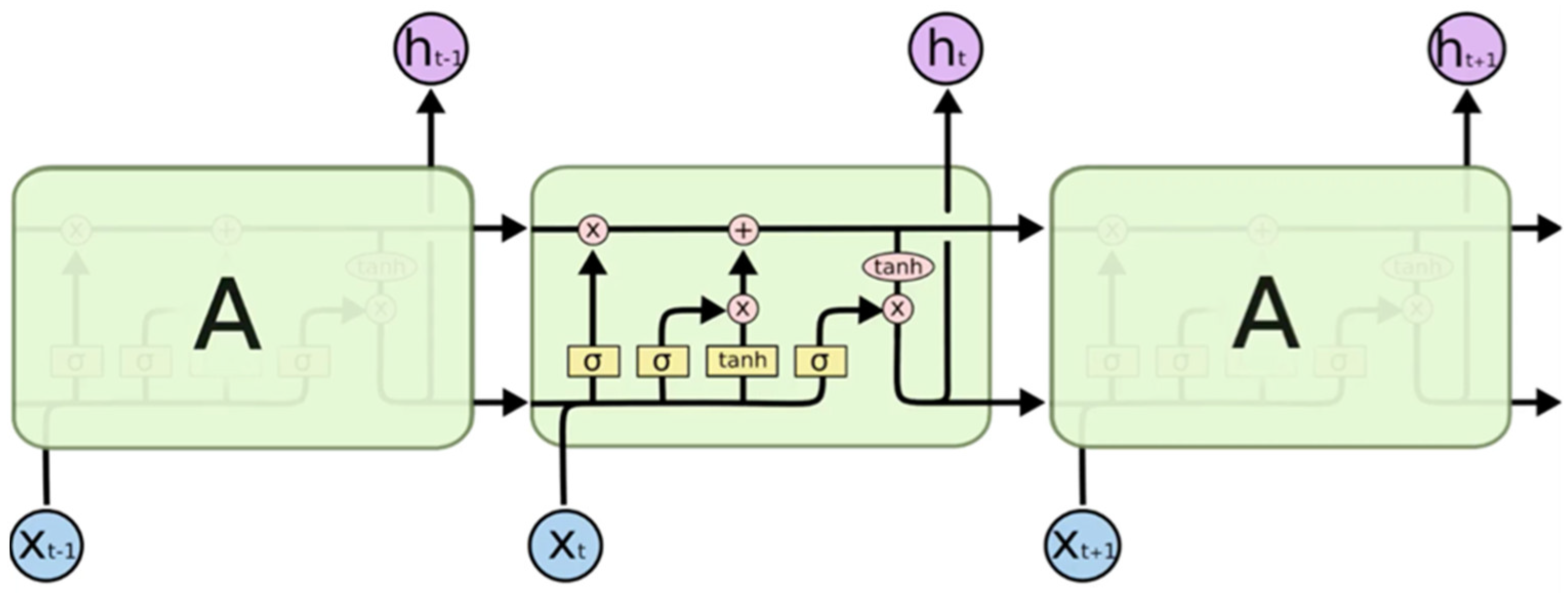
2.2.2. Long Short-Term Memory (LSTM)

The LSTM model is a specialised RNN designed to capture long-term dependencies crucial for sequence prediction. Unlike traditional neural networks [16], LSTM is adept at processing and predicting patterns in sequential data like time series, text, and speech, making it a popular choice for natural language processing and other applications in Artificial Intelligence.

Figure 2 illustrates the LSTM architecture, which includes three main parts: the forget gate (which decides the relevance of previous information), the input gate (which learns new information), and the output gate (which passes updated information to the next step). These gates regulate the information flow, aided by the hidden state (short-term memory) and cell state (long-term memory) [17]. This design enables LSTM models to process and predict patterns in entire sequences effectively.

2.2.3. Convolutional Neural Networks (CNNs)

The CNN originated in the 1980s for recognising handwritten digits but gained prominence in 2012 with Alex Krizhevsky’s work, thanks to large datasets like ImageNet and improved computing power [19,20]. Despite their success, CNNs struggle with contextual information in images. Nonetheless, they have revolutionised AI, impacting facial recognition, image search, and augmented reality.

Central to AlexNet, CNNs mimic human vision using convolution to simplify image processing while preserving essential features. They apply filters to input images, creating convolved features processed through multiple layers. Early layers detect basic features, while deeper layers identify complex elements like objects and faces [21]. The final convolution layer’s activation map informs the classification layer, producing confidence scores for image classification.

2.2.4. CNN-LSTM Hybrid Model

The CNN-LSTM hybrid model effectively combines CNNs and LSTMs to handle sequential data with spatial dependencies. This integration is ideal for time-series analysis [22], video processing, and spatiotemporal modelling.

CNNs excel at spatial feature extraction through convolutional layers, while LSTMs are skilled at capturing long-term temporal dependencies. In this hybrid model, the CNN extracts spatial features, which are then processed by the LSTM to model sequential patterns. This setup allows the model to represent both spatial and temporal dimensions comprehensively.

The CNN-LSTM hybrid is versatile and particularly useful in video analysis for recognising activities by combining spatial feature extraction with temporal modelling. It also performs well with spatiotemporal data, such as weather patterns, by capturing spatial features and modelling their evolution over time.

2.2.5. Gated Recurrent Units (GRUs)

The GRU, introduced in 2014 by Kyunghyun Cho and team, is a simplified evolution of RNNs, similar to LSTM but with a more streamlined architecture that allows for faster training. Unlike LSTM, GRUs use only a hidden state (h_t) and lack a separate cell state (Ct). They incorporate two key gates: the reset gate, which manages short-term memory, and the update gate, which handles long-term memory [23], as shown in Figure 3.

In operation, a GRU generates a candidate hidden state by combining the input (x_t) with the previous hidden state (h_t−1) using the reset gate (r_t). The update gate then balances the influence of historical and new data to produce the current hidden state (h_t) [24]. GRUs are efficient and effective in recurrent neural networks due to their simplified architecture and reliance on fewer components.

2.2.6. Multilayer Perceptron (MLP)

The MLP model features multiple layers, including a crucial hidden layer for complex data representation. When MLPs have more than one hidden layer, they are termed deep ANNs. Tuning hyperparameters like the number of layers and neurons is essential, which is often carried out through cross-validation. While back-propagation adjusts weights, deeper networks may face vanishing-gradient problems, requiring specialised algorithms [25].

MLP learning involves forward-propagation, error calculation, back-propagation, and iterative weight adjustments across epochs. During forward-propagation, hidden layer activations are computed using functions like Sigmoid, which introduces the nonlinearity necessary for complex tasks like image processing.

Figure 4 shows that paying attention to weight initialisation methods, such as Xavier/Glorot, is critical to avoid vanishing or exploding gradients, especially in deep networks. Regularisation strategies like dropout help combat overfitting and improve model generalisation. Though they have historically used Sigmoid functions, MLPs now often use Rectified Linear Unit (ReLU) activations for better nonlinearity, sparse activations, and reduced vanishing-gradient issues. This evolution in activation functions reflects a balance between computational efficiency and expressive power.

2.3. Comparison between Models

Table 1. Strengths and weaknesses of different predictive models.

Model	Application	Strengths	Weaknesses
RNN	Sequential data and time-series analysis	Captures temporal dependencies. Simple architecture. Can handle variable-length sequences.	Vulnerable to vanishing/exploding-gradient problems in long sequences. Struggles with very-long-term dependencies due to its limited memory. Computationally intensive.
LSTM	Sequence modelling, time-series prediction, natural language processing	Effectively captures long-term dependencies. Guards against vanishing-gradient problem in RNNs. Suitable for sequential tasks with variable-length inputs/outputs.	More computationally intensive than simpler models. Prone to overfitting with small datasets.
CNN	Image application and video analysis; grid-like data processing	Effective at capturing spatial dependencies. Handles local patterns well. Reduces the number of parameters through parameter sharing.	Limited ability to capture long-term dependencies in sequential data. Fixed input size.
CNN-LSTM hybrid	Tasks with spatial and temporal aspects	Captures spatial features with its CNN. Captures sequential patterns with its LSTM. Suitable for tasks where both image and time-series information are essential.	Increased complexity compared to standalone models. Requires more training data.
GRU	Sequence modelling: similar to LSTM but more computationally efficient	Handles long-term dependencies. More computationally efficient than LSTM.	Struggles with capturing very-long-term dependencies. Less expressive than LSTM.
MLP	Various tasks, including classification and regression	Simple architecture. Suitable for tasks with well-defined input–output mappings. Performs well on structured/tabular data.	May struggle with complex, nonlinear relationships in data. Limited ability to handle sequential/temporal patterns.

presents an insightful analysis of the strengths and weaknesses inherent in CNN, CNN-LSTM hybrid, GRU, LSTM, MLP, and RNN models [27]. This comprehensive overview assists in identifying the specific domains where each model excels and where it might face limitations, guiding its practical application.

2.4. Evaluation Metrics

Three error metrics are commonly used to measure errors, also referred to as residual values, in order to evaluate and report regression model performance:

• Mean Absolute Error:

MAE is a metric that quantifies the average absolute differences between predicted and actual values [3]. It is calculated by taking the average absolute differences between the predicted and actual values. The formula for MAE is as follows:

$$MAE={\displaystyle \frac{1}{n}}{{\displaystyle \sum }}_{i=1}^n\left|y_i-{\widehat{y}}_i\right|$$

(1)

where

• $n$: is the number of observations;
• $y_i$: is the actual value;
• ${\widehat{y}}_i$: is the predicted value.

A lower MAE indicates better accuracy, which signifies more minor errors between the predicted and actual values.

• Mean Squared Error:

MSE measures the average of the squared differences between predicted and actual values. It is obtained by squaring the individual errors, emphasising more significant errors over smaller ones [28]. The formula for MSE is as follows:

$$MSE={\displaystyle \frac{1}{n}}{{\displaystyle \sum }}_{i=1}^n{(y_i-{\widehat{y}}_i)}^2$$

(2)

Similar to MAE, a lower MSE is desirable, indicating a more accurate model.

• Mean Absolute Percentage Error:

MAPE calculates the percentage difference between predicted and actual values, providing a relative measure of accuracy [29]. The formula for MAPE is as follows:

$$MAPE={\displaystyle \frac{1}{n}}{{\displaystyle \sum }}_{i=1}^n\left({\displaystyle \frac{\left|y_i-{\widehat{y}}_i\right|}{\left|y_i\right|}}\right)\times 100\%$$

(3)

A lower MAPE indicates a more accurate model regarding the percentage difference between predicted and actual values. MAPE is particularly useful when you want to understand the accuracy relative to the scale of the actual values.

3. Research Objective

The primary objective of this study is to develop and evaluate machine learning models for predicting project completion times in the context of project management. Project timelines’ dynamic and multifaceted nature poses a significant challenge for accurate forecasting, necessitating the exploration of advanced computational techniques. This study aims to address the following key aspects:

• To precisely assess the performance of LSTM, CNN, CNN-LSTM, GRU, MLP, and RNN models in predicting project completion time, required personnel, and estimated costs. This involves utilising a comprehensive dataset that reflects the complexities of real-world projects to determine how well each model can forecast these crucial project parameters.
• To compare the accuracy of these models using specific evaluation metrics: MAE, MSE, and MAPE. This comparison aims to provide a detailed understanding of each model’s predictive precision, aiding in selecting the most accurate model for project management.
• To determine which machine learning architecture (LSTM, CNN, CNN-LSTM, GRU, MLP, RNN) best predicts project parameters. The goal is to identify the most effective model for different project scenarios and data patterns, thereby supporting more reliable forecasting.
• To elucidate each model’s strengths and limitations, focusing on its ability to handle various project types and complexities. This will help us understand which models are best suited for different project characteristics and provide insights into potential areas for improvement.
• To offer actionable insights for refining predictive models and exploring advanced techniques, such as ensemble methods and hyperparameter optimisation. This objective aims to improve prediction accuracy and robustness in project management.
• To assist students and project managers in ensuring the success of their projects by providing accurate predictions for project completion times and required resources. This includes offering guidance on measuring, estimating, and managing timeframes effectively, enhancing project planning and execution.
• To evaluate the practical implications of the resulting model predictions for real-world project management. This involves understanding how these predictive models can be applied to improve decision-making, resource allocation, and overall project success.

This research aims to advance the field of project management by integrating and evaluating advanced machine learning techniques and introducing novel hybrid models and preprocessing strategies, thereby providing a comprehensive understanding of their effectiveness and practical implications.

4. Related Work

Filippettoet al. [30] introduced the Atropos model, a comprehensive framework for risk prediction in software project management. The model utilises historical project contexts and similarity analysis to provide risk recommendations tailored to new projects. Integrating concepts from ubiquitous computing, agile methodologies, and activity theory, Atropos enhances stakeholder collaboration, quantifies risks, and prioritises them effectively. It addresses all phases of risk management, including identification, analysis, and mitigation, with a strong focus on improving decision-making and reducing project failure rates. Future work aims to refine and validate this model’s effectiveness across various projects.

Malgonde and Chari [31] proposed an ensemble-based predictive model for effort estimation in agile software development. The model integrates various predictive algorithms to enhance accuracy and is particularly useful in sprint planning and effort optimisation. Their research identifies key predictor variables: effort, priority, subtasks, size, sprint, and programmer experience. The ensemble-based approach is demonstrated to improve estimation accuracy, providing valuable insights for project managers. The study also outlines limitations and future research directions to refine the model further.

Pasuksmit et al. [32] introduced DocWarn-H, a hybrid model for predicting documentation changes in agile development. This model combines metrics from DocWarn-C with contextualised text vectors from DocWarn-T, trained using a neural network. The study highlights the importance of predicting documentation changes to manage uncertainty and support effort estimation and sprint planning. By analysing multiple software projects, the authors demonstrate that specific work item characteristics can predict documentation changes, providing a valuable tool for agile teams.

Licorish et al. [33] explored the challenges of prioritising app feature fixes using user reviews. Their study reveals that traditional requirement-engineering methods are insufficient for application development, which relies heavily on post-release user feedback. Through content analysis and regression, they found that reviews often lack actionable information but can indicate severe functionality issues. The study emphasises redesigning app review interfaces to better capture valuable feedback. Future research is suggested to employ deep learning techniques for improved review mining and feature prioritisation.

Our approach further address the topics in [30,31], by utilising various machine learning models and providing their analysis and comparison.

5. Study Methodology

This study’s methodology is designed to explore predictive modelling in project management comprehensively. Focusing on students affiliated with the Department of Computers and Informatics at the Technical University of Košice [34], this study aims to assess various predictive models’ efficacy in forecasting critical project parameters. These include the completion time, persons needed, and estimated costs, catering to the dynamic nature of real-world project management scenarios. The following provides an overview of the dataset, highlighting key attributes and laying the groundwork for evaluating model predictions. Subsequently, the exploration unfolds through tables showcasing the original dataset and predicted outcomes from diverse machine learning models.

5.1. Data Collection

This study involved distributing a meticulously crafted questionnaire via Google Forms to a targeted group of students affiliated with the Department of Computers and Informatics at the Technical University of Košice. The questionnaire was tailored for students in their final classes, focusing on informatics and software development.

5.1.1. Data Collection Process

A meticulous approach was paramount in orchestrating our investigation into project management methodologies to ensure robust data acquisition.

• We distributed the questionnaire on electronic platforms associated with the academic bodies mentioned above.
• We obtained responses from students, totaling 190 responses.
• We performed data checking and cleaning, including removing incomplete or incomprehensible responses.
• We classified the collected data into two main groups: students following the waterfall methodology and those adopting the agile method.
• Data classification was based on project parameters such as the project type, team size, expected completion time, and project overview.

5.1.2. Respondent Selection

This study employed purposive sampling. The following criteria were used to select respondents:

• Affiliation: Only students from the Department of Computers and Informatics at the Technical University of Košice were selected.
• Academic Standing: Respondents needed to be in their final classes, ensuring they had sufficient knowledge and experience in informatics and software development.
• Experience with Project Management: Students who had completed at least one project management course or had practical experience were targeted.
• Project Methodology: Respondents were selected based on their familiarity with the waterfall or agile project management methodologies.

5.2. Consent and Personal Data Protection

Ethical considerations related to consent and personal data protection were paramount in this study. We researchers took several steps to ensure that respondents’ data were protected and their participation was voluntary and informed. Before data collection began, all potential respondents were provided with detailed study information.

• One of the project team members provided the students with a detailed explanation of the study. This session included information about the study’s objectives, the nature of the data being collected, and how the data would be used.
• The study was also distributed on one of the university’s documented platforms, ensuring that all information was accessible to the students.
• Participants were assured that their responses would be kept confidential and that any published results would not include identifiable information.
• All collected data were anonymised to ensure that individual respondents could not be identified from the dataset.

5.3. Machine Learning Models

This study employed machine learning models to predict project completion times, offering a comprehensive understanding of the data. The models used included CNN, CNN-LSTM hybrid, GRU, LSTM, MLP, and RNN models. Each model has distinct architectures and capabilities, making it suitable for diverse data patterns and complexities.

5.4. Training and Evaluation Process for Each Model

The training and evaluation of each machine learning model followed a standardised procedure:

• Data splitting: The dataset was split into training and testing sets to assess the models’ generalisation performance accurately. An 80–20 split was adopted, allocating 80% of the data for training and 20% for testing.
• Model curation: Distinct models were used for each machine learning architecture, incorporating unique layer configurations. For instance, the CNN model featured convolutional layers for spatial feature extraction, while the LSTM model emphasised sequential data understanding.
• Training: Models underwent an iterative training process using the training set. The training involved minimising a predefined loss function, adjusting model weights through back-propagation, and optimising performance over multiple epochs.
• Prediction: After training, each model was evaluated on the testing set to simulate real-world predictive scenarios, and predictions were generated for project completion times based on the patterns learned from the training data.
• Evaluation metrics: Each model’s performance was quantified using standard evaluation metrics such as MAE, MSE, and MAPE. These metrics provided insights into the accuracy and reliability of the models in predicting project completion times.

6. Results and Analysis

This section will examine the outcomes derived from our predictive model, which has been meticulously crafted with versatility in mind. The architecture incorporates a combination of recurrent and convolutional layers strategically chosen to adeptly capture temporal and sequential patterns inherent in project features. Our model comprises simple RNN, LSTM, GRU, CNN, and hybrid CNN-LSTM architecture, offering adaptability to various project dynamics.

The selection of the algorithms driving our model’s effectiveness was based on their demonstrated efficacy in handling sequential and temporal data. The CNN, LSTM, GRU, and hybrid models were explicitly chosen for their ability to discern patterns within diverse project datasets. Introducing a hybrid CNN-LSTM model aimed to leverage the strengths of both convolutional and recurrent layers, potentially uncovering intricate patterns within project-related features. In implementing these architectures, we utilised TensorFlow’s Keras API, providing a robust and efficient deep learning framework. The model was continually refined throughout development until we achieved optimal effectiveness within our dataset.

6.1. “Predicted Completion Time” Results

Table 2. The results pertaining to the “predicted completion time” (days) for each model.

Project Name	Original Dataset	Predicted Results
	Expected Duration	LSTM	CNN-LSTM	CNN	GRU	MLP	RNN
GPS	90	66	64	68	67	64	60
Web app	90	68	63	68	67	63	64
Smart clock	90	60	59	66	66	64	63
Web game	90	70	68	66	66	68	64
Desktop blog app	90	72	72	66	67	66	64
Web-based game	90	77	65	68	66	74	63
Web application	90	65	69	66	68	71	59
Custom	90	63	68	68	67	62	68
Unity game	90	60	64	67	67	71	72
Lights Out game	90	71	58	67	66	60	65
Web application for posting blogs	90	73	73	66	68	64	63
School project	90	67	80	67	67	63	64
Blog web application with a simple UI	90	68	72	67	68	64	68
Mobile app to support and automate FP+COCOMO calculations	90	80	63	68	67	66	71
Shazam application	90	77	64	67	67	74	62
App for management of save files	60	62	68	67	66	71	71
Simple service for users, sound recognition	90	58	66	66	68	62	60

compares the original dataset’s expected duration and the predicted completion times generated by various machine learning models, namely LSTM, CNN-LSTM, CNN, GRU, MLP, and RNN, for multiple projects. The original dataset’s expected duration serves as a benchmark for evaluating the accuracy and reliability of the predictive models.

The results can be used to explore the potential reasons for variations across models and highlight practical outcomes for project management.

The LSTM model generally predicted completion times lower than the expected duration (e.g., “66 days” for “GPS” compared to the expected “90 days”). This tendency suggests that LSTM might be capable of capturing the essential features that drive completion time but may underestimate the impact of some factors, possibly due to its focus on time-series patterns rather than project-specific complexities. For instance, LSTM predicted “65 days” for “Web application”, significantly lower than the expected “90 days”. This may indicate that the LSTM model perceives these projects as less complex than they are, possibly due to oversimplification in its learned patterns.

CNN-LSTM predictions are often close to the LSTM predictions but show more variability. For example, in the “Web-based game” project, CNN-LSTM predicted “65 days” compared to LSTM’s “77 days”. This variation might arise from the CNN component, which could capture different project features that influence the timeline, such as dependencies and concurrent tasks, leading to more accurate or varied predictions depending on the project’s nature. This model seems to be slightly more sensitive to project complexity, leading to a broader range of predictions. For instance, for the “School project”, CNN-LSTM predicted “80 days”, significantly deviating from LSTM’s “67 days” and being closer to the expected duration, indicating its ability to detect project-specific nuances.

The CNN model predicted completion times generally higher than those predicted by LSTM and CNN-LSTM (e.g., “68 days” for “GPS”). This might be due to the CNN’s architecture, which excels at capturing complex patterns in data, potentially identifying project details that other models overlook. The CNN consistently predicted “67 or 68 days” for many projects, suggesting it accounts for additional complexities, such as resource constraints or task interdependencies, that simpler models might not fully capture.

The GRU and MLP models show mixed performances, with predictions sometimes close to the expected duration (e.g., “67 days” for “GPS” by GRU) but also with noticeable underestimations (e.g., “63 days” for “Custom” by MLP). These models may struggle with capturing the full complexity of project timelines, especially for more intricate projects, resulting in generally lower predictions than the expected duration. For example, MLP’s prediction of “62 days” for the “Custom” project indicates a potential underestimation of the project scope or complexities.

The RNN’s predictions are often lower than other models (e.g., “60 days” for “GPS”). The RNN model may be overly influenced by short-term patterns in the data, leading to optimistic predictions that do not fully account for all project phases. The prediction for “Web application” (59 days) is particularly low, which might indicate that this RNN could not fully capture the challenges inherent in web development projects, such as iterative testing or debugging.

For projects like “Web application for posting blogs”, predictions across the models vary widely. CNN-LSTM and LSTM predicted “73 days”, close to the expected “90 days”, while the RNN predicted “63 days”. This suggests that models like LSTM and CNN-LSTM, which combine temporal and feature-based learning, are better suited for these types of projects.

In custom projects like the “Shazam application”, CNN-LSTM predicted “64 days”, while LSTM predicted “77 days”. The deviation could indicate the models’ sensitivity to unique project characteristics. For custom or novel projects, using a model that can handle both temporal patterns and specific features (like CNN-LSTM) might be advantageous for a more accurate timeline estimation.

Predictions vary significantly for game development projects (e.g., “Unity game” and “Web game”), with LSTM predicting “60 days” for “Unity game”, whereas CNN-LSTM and CNN predicted longer durations. This variability highlights the complexity and unpredictability of game development projects, where different models might capture various aspects of the development process.

In Figure 5, a statistical summary showcases the median, quartiles, and potential outliers in the predicted completion time results.

Figure 6 illustrates the predicted completion time (days) across various models compared to the original expected duration from the dataset. Each line represents a dataset, showcasing how well the models align with the project durations.

6.2. “Persons Needed” Results

Table 3. The results pertaining to the “persons needed” for each model.

Project Name	Original Dataset	Predicted Results
	Team Size	LSTM	CNN-LSTM	CNN	GRU	MLP	RNN
GPS	2	4	3	5	5	8	8
Web app	5	8	2	5	5	2	3
Smart clock	3	1	5	5	3	5	1
Web game	3	5	1	2	3	4	5
Desktop blog app	2	5	1	2	8	5	2
Web-based game	3	2	2	2	3	1	2
Web application	1	5	8	1	2	2	2
Custom	1	8	8	4	2	4	2
Unity game	1	3	2	4	2	4	2
Lights Out game	3	4	3	5	3	8	3
Web application for posting blogs	2	5	1	8	2	4	5
School project	4	8	2	1	2	2	1
Blog web application with a simple UI	5	3	4	2	4	2	3
Mobile app to support and automate FP+COCOMO calculations	3	4	4	5	5	8	5
Shazam application	3	3	5	5	8	4	4
App for management of save files	5	3	8	5	5	2	1
Simple service for users, sound recognition	1	3	1	5	5	1	1

compares the original dataset’s team sizes and the predicted number of persons needed for various projects, as estimated by different machine learning models, including LSTM, CNN-LSTM, CNN, GRU, MLP, and RNN. The original dataset’s team size serves as a reference for evaluating the accuracy and reliability of the predictive models.

The results explore possible reasons for specific predictions and their practical implications for project management.

LSTM predictions for team size tend to be higher than the original dataset. For instance, LSTM predicted that four people were needed for the “GPS” project, compared to the original two. This pattern suggests that LSTM might overestimate the required team size, potentially due to its sensitivity to the complexity of project phases and the involvement needed at each step. However, LSTM sometimes underestimates the team size, as seen in the “Smart clock” project, where it predicted one person compared to the original three. This discrepancy could be due to the model underestimating the variety of tasks or underappreciating the need for a diverse skill set.

CNN-LSTM shows significant variability, predicting as few as one person for the “Web-based game”, in line with the original dataset, but also overestimating for other projects, like “Custom”, where it predicted eight people compared to the original one. This variability might be due to the CNN-LSTM model capturing complex patterns related to team dynamics but possibly overfitting certain project features, leading to inconsistent predictions across different projects.

CNN predictions vary widely, with some predictions closely matching the original dataset (e.g., two for the “Web app” and five for “GPS”) and others showing significant overestimation, such as eight for the “Web application for posting blogs” compared to the original two. The CNN model might focus on specific project aspects like the number of tasks, dependencies, or required skills, leading to larger predicted team sizes for projects where these factors are prominent.

The GRU and MLP models also show a range of predictions, from underestimating the team size (e.g., one person for the “school project” according to the GRU model compared to the original four) to overestimating it (e.g., eight people for the “Desktop blog app” according to MLP compared to the original two). These models might have struggled with generalising across different project types, leading to predictions that vary significantly depending on how the model interprets the complexity and scope of each project.

The RNN predictions are quite varied, often matching the original dataset (e.g., two for the “Desktop blog app” and one for the “Simple service for users, sound recognition”) but also showing overestimation in some cases, like its prediction of eight people for “GPS”. The RNN model may have been overly influenced by specific features or patterns within the training data, leading to inconsistent predictions across different projects.

For smaller projects like “GPS” or the “Simple service for users, sound recognition”, the predicted team sizes vary widely. The LSTM and CNN tend to predict more team members than necessary, which could suggest that these models are sensitive to perceived complexity that may not exist. For instance, the CNN predicted “five” people for the “Simple service for users”, which is higher than the original “one” person, indicating a possible misinterpretation of this project as requiring more resources.

For web-based projects such as the “Web application for posting blogs”, predictions are again inconsistent. The CNN predicted eight people, far exceeding the original two, which could indicate an overestimation of this project’s complexity or the resources needed to manage and execute web development tasks. On the other hand, CNN-LSTM predicted one person, which aligns with the original dataset, showing that while CNN-LSTM might overestimate for some projects, it can also provide accurate estimates depending on the data it captures.

Predictions for custom and specialised projects like the “Shazam application” or “App for management of save files” vary significantly. LSTM predicted three people for the “Shazam application”, which is the same as the original, but CNN-LSTM predicted five, possibly indicating that CNN-LSTM needs more specialised roles in such projects. Similarly, MLP’s prediction of eight people for the “App for management of save files” compared to the original five might reflect an overestimation of this project’s complexity or the perceived need for a larger, more diverse team.

The CNN and CNN-LSTM models demonstrated a strong understanding of individual needs, providing consistent estimates. In contrast, the GRU, MLP, and RNN models exhibited some variability, indicating potential areas for improvement in staffing predictions, as illustrated in Figure 7 and Figure 8.

6.3. “Estimated Cost” Results

Table 4. The result pertaining to the “estimated cost” for each model.

Project Name	Predicted Results
	LSTM	CNN-LSTM	CNN	GRU	MLP	RNN
GPS	170	171	170	169	169	170
Web app	170	172	170	169	169	170
Smart clock	165	168	165	166	165	165
Web game	164	168	165	166	164	165
Desktop blog app	170	170	165	169	169	170
Web-based game	165	168	170	166	166	165
Web application	170	174	166	170	171	170
Custom	169	170	170	169	169	169
Unity game	169	169	169	169	169	169
Lights Out game	165	166	169	166	166	165
Web application for posting blogs	171	169	165	170	170	171
School project	167	169	168	168	167	167
Blog web application with a simple UI	171	173	167	170	170	171
Mobile app to support and automate FP+COCOMO calculations	170	170	169	169	169	170
Shazam application	167	169	170	168	167	167
App for management of save files	170	170	167	169	169	170
Simple service for users, sound recognition	164	169	169	166	166	165

presents the results for the “estimated cost” across different projects as predicted by various machine learning models: LSTM, CNN-LSTM, CNN, GRU, MLP, and RNN.

The LSTM model shows highly consistent predictions across most projects, frequently predicting the exact cost (e.g., “170” for projects like the “GPS”, “Web app”, and “Desktop blog app” projects). This consistency suggests that LSTM effectively suits scenarios with clear and predictable project requirements. The stable predictions indicate that LSTM can reliably generalise from the training data, making it a dependable model for estimating costs in typical projects.

The CNN-LSTM model predicted slightly higher costs than LSTM (e.g., “171” or “172” compared to LSTM’s “170” for the same projects). This difference could stem from CNN-LSTM’s architecture, which includes convolutional layers that may capture more detailed features of the projects, such as hidden complexities or nuances, leading to higher cost estimates. For example, the higher prediction for “Web application” (“174” vs. “170”) might indicate that CNN-LSTM is sensitive to subtle project-specific details that LSTM overlooks.

The CNN predictions are generally close to LSTM’s but occasionally differ slightly (e.g., 170 for "GPS" and "Web app" but 165 for "Desktop blog app"). This suggests that while CNN captures relevant patterns, its performance may vary depending on the project type.

The GRU also shows consistency, similar to LSTM, with slight deviations (e.g., predicting 169 for the "GPS" and "Web app" projects). GRU’s ability to handle sequential data effectively is reflected in its stable predictions, although it occasionally predicts lower costs than LSTM and CNN-LSTM.

The MLP and RNN models show a mixed performance. While their predictions often align with LSTM’s predictions, they occasionally deviate (e.g., MLP predicting “171” for the “Web application”). This variability might be due to the simpler architecture of the MLP and RNN models, which may struggle with capturing complex relationships between features, leading to slight overestimations or underestimations.

For web-based projects like the “Web app”, “Web-based game”, and “Web application”, predictions across models are quite consistent. This consistency suggests that these project types share common characteristics that the models effectively learned, resulting in stable predictions. For example, the predictions for the “Web-based game” are closely aligned, with minimal variation among the models, indicating the models’ proficiency in handling such projects.

In projects related to game development (the “Web game”, “Unity game”, and “Lights Out game”), the predictions vary more significantly. For example, the LSTM model predicted “164” for the “Web game”, whereas CNN-LSTM and MLP predicted “168”. This variation could reflect the complexity and unpredictability inherent in game development, where different models interpret the project’s scope differently, leading to variations in estimated costs.

Predictions for custom projects (e.g., the “Shazam application” and “Simple service for users”) show slight variations across models, indicating the challenges in accurately estimating costs for non-standard, unique projects. For instance, the CNN-LSTM model’s slightly higher predictions may be due to its ability to detect hidden complexities that simpler models like MLP might miss, as shown in Figure 9.

6.4. Comparison of Metrics across Models

We present a detailed evaluation of the predictive performance of six distinct models, CNN, CNN-LSTM hybrid, GRU, LSTM, MLP, and RNN, using key evaluation metrics; these metrics offer a comprehensive insight into the accuracy and reliability of each model in predicting critical project parameters, as shown in

Table 5. Evaluation metrics for predictive models in project management.

Model	MAE (avg.)	MSE (avg.)	MAPE (avg.)
CNN	0.023	0.001	5.8%
CNN-LSTM hybrid	0.037	0.002	9.2%
GRU	0.027	0.001	6.7%
LSTM	0.036	0.002	9.0%
MLP	0.016	0.000	4.0%
RNN	0.009	0.000	2.2%

.

Figure 10 illustrates the comparative performance of these models across the three metrics. We report the key findings from our evaluation as follows.

6.4.1. Mean Absolute Error

Here are the results regarding the MSE metric, which sheds light on each model’s comparative performance in minimising absolute error, as shown in Figure 11.

• The RNN stands out as the top-performing model, with the lowest MAE of 0.0056. The MLP and GRU models also demonstrate excellent performance, with MAE values of 0.0175 and 0.0202, respectively.
• The CNN and LSTM models exhibit slightly higher MAE values but remain competitive, showcasing their competence in minimising prediction errors.
• CNN-LSTM hybrid, while still effective, shows a comparatively higher MAE.

6.4.2. Mean Squared Error

Here, we will explore the findings regarding the MSE, which will shed light on each model’s comparative performance in minimising squared errors. This exploration will offer valuable insights into the efficacy of different approaches in handling predictive tasks, as shown in Figure 12.

• The RNN again leads with the lowest MSE of 0.0001, emphasising its superior ability to minimise squared errors.
• The MLP and GRU models follow closely with impressive MSE values of 0.000580942 and 0.000505865, respectively.
• The CNN model, LSTM model, and CNN-LSTM hybrid model display higher MSE values but maintain effectiveness in reducing squared errors.

6.4.3. Mean Absolute Percentage Error

Delving into the comprehensive findings from the MAPE analysis, we uncover valuable insights into each model’s performance, specifically its ability to provide percentage errors accurately, as shown in Figure 13.

• The RNN exhibits exceptional accuracy, with the lowest MAPE of 1.39%, indicating its proficiency in providing precise percentage errors.
• MLP and CNN-LSTM hybrid also perform well, demonstrating MAPE values of 4.36% and 9.21%, respectively.
• While slightly higher in MAPE, the CNN, GRU, and LSTM models effectively minimise percentage errors.

Among the evaluated models, the RNN consistently performs exceptionally well across all metrics, showcasing its proficiency in minimising prediction errors and providing accurate estimates. The MLP and GRU models also demonstrate strong performance, while the CNN and LSTM remain competitive, albeit with slightly higher errors. The MAE, MSE, and MAPE comparison charts visually illustrate these model performances.

7. Conclusions

In conclusion, this comprehensive evaluation of diverse predictive models for project management has provided valuable insights into their strengths and areas for improvement. The success of models such as the LSTM, CNN, CNN-LSTM, GRU, MLP, and RNN models in forecasting critical project parameters, including completion time, required personnel, and estimated costs, underscores the robustness of these models in capturing intricate patterns within the dataset.

The comparative analysis revealed a remarkable consistency and close alignment of results across various models, highlighting their collective ability to provide reliable predictions.

Notably, the LSTM model emerges as a pinnacle of success, demonstrating exceptional accuracy and reliability in predicting completion time, persons needed, and estimated costs. While RNNs exhibit lower MAE, MSE, and MAPE values in this study, indicating strong performance on the evaluated metrics, LSTMs offer distinct advantages in handling the complex and long-term dependencies inherent in project management data. Their superior capability to manage long-term temporal relationships and adaptability to varying data complexities make them more suitable for comprehensive and robust project management predictions, even if they demonstrate slightly higher average metrics in specific evaluations.

LSTM’s consistent performance across diverse projects underscores its versatility, and this research aimed to conduct a thorough investigation into predictive modelling as it relates to project management. The ultimate objective was to assess the efficacy of different predictive models in forecasting crucial project parameters, including completion time, necessary personnel, and estimated costs. The studied models have been specifically designed to accommodate the ever-evolving nature of real-world project management scenarios. The introduction offers an overview of the dataset, highlighting key features and laying the foundation for evaluating model predictions. Subsequently, the study unfolds through tables that present the original dataset and predicted results from various machine learning models as well as evaluation metrics to gain a nuanced understanding of model performance. As the predictive modelling landscape evolves, the success observed in this study encourages ongoing refinement, the exploration of ensemble strategies, and further optimisation of hyperparameters to enhance predictive accuracy in the dynamic realm of project management.

This research’s findings are applicable to a wide range of industry scenarios and are particularly valuable for educational purposes. By focusing on predictive modelling and project management, this study offers a robust framework that can be utilised to teach university students how to work in teams effectively. The models and methods explored here can serve as powerful tools to help students understand and navigate the complexities of real-world projects, preparing them for future professional challenges; the primary focus is on providing university students with the tools and knowledge to work effectively in teams and successfully complete their projects. From the point of view of industry managers and staff engineers, the predictions for small task groups are suitable for scheduling improvements of effort distribution across several projects being solved in parallel.

Future research will expand the dataset used in this study to include a broader range of projects and industry contexts. This will help assess the generalisability of the models and ensure their applicability across diverse scenarios. Additionally, further exploration of hybrid models could yield improvements in performance metrics. Experimenting with new hybrid architectures or enhancements, alongside advanced feature engineering techniques, will refine model accuracy and robustness. Longitudinal studies could also provide insights into how these models perform over extended periods and different project phases, revealing their long-term reliability.

References

1. Yang, Y.; Xia, X.; Lo, D.; Bi, T.; Grundy, J.; Yang, X. Predictive Models in Software Engineering: Challenges and Opportunities. arXiv 2020, arXiv:2008.03656. Available online: http://arxiv.org/abs/2008.03656 (accessed on 10 August 2024). [CrossRef]
2. Wang, Q. How to apply AI technology in Project Management. PM World J. 2019, VIII, 1–12. [Google Scholar]
3. Chicco, D.; Warrens, M.J.; Jurman, G. The coefficient of determination R-squared is more informative than SMAPE, MAE, MAPE, MSE and RMSE in regression analysis evaluation. PeerJ Comput. Sci. 2021, 7, e623. [Google Scholar] [CrossRef]
4. Auth, G.; Jokisch, O.; Dürk, C. Revisiting automated project management in the digital age—A survey of AI approaches. Online J. Appl. Knowl. Manag. 2019, 7, 27–39. [Google Scholar] [CrossRef]
5. Martínez-Fernández, S.; Bogner, J.; Franch, X.; Oriol, M.; Siebert, J.; Trendowicz, A.; Vollmer, A.M.; Wagner, S. Software Engineering for AI-Based Systems: A Survey. ACM Trans. Softw. Eng. Methodol. 2022, 31, 37e. [Google Scholar] [CrossRef]
6. McGrath, J.; Kostalova, J. Project Management Trends and New Challenges 2020+. Hradec Econ. Days 2020, 10, 534–542. [Google Scholar] [CrossRef]
7. Bodimani, M. AI and Software Engineering: Rapid Process Improvement through Advanced Techniques. J. Sci. Technol. 2021, 2, 95–119. [Google Scholar]
8. Hofmann, P.; Jöhnk, J.; Protschky, D.; Urbach, N. Developing Purposeful AI Use Cases—A Structured Method and Its Application in Project Management. In Proceedings of the 15th International Conference on Wirtschaftsinformatik (WI) (WI2020), Postdam, Germany, 9–11 March 2020; pp. 33–49, ISBN 978-3-95545-335-0. [Google Scholar]
9. Khan, A. Artificial Intelligence (AI) Techniques. Available online: https://intellipaat.com/blog/artificial-intelligence-techniques/ (accessed on 5 March 2024).
10. Anitha, N.N.S.; Reddymalla, N.R.; Karri, V.R. Introduction of Artificial Intelligence techniques and approaches. Asian J. Multidiscip. Stud. 2020, 8, 15–24. [Google Scholar]
11. Sarker, I.H. AI-Based Modeling: Techniques, Applications and Research Issues Towards Automation, Intelligent and Smart Systems. SN Comput. Sci. 2022, 3, 158. [Google Scholar] [CrossRef]
12. Bouwmans, T.; Javed, S.; Sultana, M.; Jung, S.K. Deep neural network concepts for background subtraction: A systematic review and comparative evaluation. Neural Netw. 2019, 117, 8–66. [Google Scholar] [CrossRef]
13. Yu, Y.; Si, X.; Hu, C.; Zhang, J. A Review of Recurrent Neural Networks: LSTM Cells and Network Architectures. Neural Comput. 2019, 31, 1235–1270. [Google Scholar] [CrossRef] [PubMed]
14. Schmidt, R.M. Recurrent Neural Networks (RNNs): A Gentle Introduction and Overview. arXiv 2019, arXiv:1912.05911. Available online: http://arxiv.org/abs/1912.05911 (accessed on 29 July 2024).
15. Bianchi, F.M.; Maiorino, E.; Kampffmeyer, M.C.; Rizzi, A.; Jenssen, R. An Overview and Comparative Analysis of Recurrent Neural Networks for Short Term Load Forecasting. arXiv 2017, arXiv:1705.04378. [Google Scholar]
16. Muhammad, A.; Külahcı, F.; Salh, H.; Hama Rashid, P.A. Long Short Term Memory networks (LSTM)-Monte-Carlo simulation of soil ionization using radon. J. Atmos. Sol. Terr. Phys. 2021, 221, 105688. [Google Scholar] [CrossRef]
17. Staudemeyer, R.C.; Morris, E.R. Understanding LSTM—A Tutorial into Long Short-Term Memory Recurrent Neural Networks. arXiv 2019, arXiv:1909.09586. Available online: http://arxiv.org/abs/1909.09586 (accessed on 29 July 2024).
18. Lynn, H.M.; Pan, S.B.; Kim, P. A Deep Bidirectional GRU Network Model for Biometric Electrocardiogram Classification Based on Recurrent Neural Networks. IEEE Access 2019, 7, 145395–145405. [Google Scholar] [CrossRef]
19. Li, Z.; Liu, F.; Yang, W.; Peng, S.; Zhou, J. A Survey of Convolutional Neural Networks: Analysis, Applications, and Prospects. IEEE Trans. Neural Netw. Learn. Syst. 2022, 33, 6999–7019. [Google Scholar] [CrossRef]
20. Rosebrock, A. Deep Learing for Computer Vision. PYIMAGESEARCH. 2017. Available online: https://pyimagesearch.com/deep-learning-computer-vision-python-book/ (accessed on 9 July 2024).
21. Mandal, M. Introduction to Convolutional Neural Networks (CNN), Analytics Vidhya. 2021. Available online: https://www.analyticsvidhya.com/blog/2021/05/convolutional-neural-networks-cnn/ (accessed on 5 March 2024).
22. Abdallah, M.; An Le Khac, N.; Jahromi, H.; Delia Jurcut, A. A Hybrid CNN-LSTM Based Approach for Anomaly Detection Systems in SDNs. In Proceedings of the 16th International Conference on Availability, Reliability and Security, Vienna, Austria, 17–20 August 2021; ACM: New York, NY, USA, 2021; pp. 1–7. [Google Scholar]
23. Zargar, S.A. Introduction to Sequence Learning Models: RNN, LSTM, GRU. Agric. Philos. 2021. [Google Scholar] [CrossRef]
24. Astawa, I.N.G.A.; Pradnyana, I.P.B.A.; Suwintana, I.K. Comparison of RNN, LSTM, and GRU Methods on Forecasting Website Visitors. J. Comput. Sci. Technol. Stud. 2022, 4, 11–18. [Google Scholar] [CrossRef]
25. Li, D.; Wang, H.; Li, Z. Accurate and Fast Wavelength Demodulation for Fbg Reflected Spectrum Using Multilayer Perceptron (Mlp) Neural Network. In Proceedings of the 2020 12th International Conference on Measuring Technology and Mechatronics Automation (ICMTMA), Phuket, Thailand, 28–29 February 2020; IEEE: Piscataway, NJ, USA, 2020; pp. 265–268. [Google Scholar]
26. Abiodun, O.I.; Kiru, M.U.; Jantan, A.; Omolara, A.E.; Dada, K.V.; Umar, A.M.; Linus, O.U.; Arshad, H.; Kazaure, A.A.; Gana, U. Comprehensive Review of Artificial Neural Network Applications to Pattern Recognition. IEEE Access 2019, 7, 158820–158846. [Google Scholar] [CrossRef]
27. Shiri, F.M.; Perumal, T.; Mustapha, N.; Mohamed, R. A Comprehensive Overview and Comparative Analysis on Deep Learning Models: CNN, RNN, LSTM, GRU. arXiv 2023. [Google Scholar] [CrossRef]
28. De Myttenaere, A.; Golden, B.; Le Grand, B.; Rossi, F. Mean Absolute Percentage Error for regression models. Neurocomputing 2016, 192, 38–48. [Google Scholar] [CrossRef]
29. Prayudani, S.; Hizriadi, A.; Lase, Y.Y.; Fatmi, Y.; Al-Khowarizmi. Analysis Accuracy of Forecasting Measurement Technique on Random K-Nearest Neighbor (RKNN) Using MAPE And MSE. J. Phys. Conf. Ser. 2019, 1361, 012089. [Google Scholar] [CrossRef]
30. Filippetto, A.S.; Lima, R.; Barbosa, J.L.V. A risk prediction model for software project management based on similarity analysis of context histories. Inf. Softw. Technol. 2021, 131, 106497. [Google Scholar] [CrossRef]
31. Malgonde, O.; Chari, K. An ensemble-based model for predicting agile software development effort. Empir. Softw. Eng. 2019, 24, 1017–1055. [Google Scholar] [CrossRef]
32. Pasuksmit, J.; Thongtanunam, P.; Karunasekera, S. Towards Reliable Agile Iterative Planning via Predicting Documentation Changes of Work Items. In Proceedings of the 19th International Conference on Mining Software Repositories, Pittsburgh, PA, USA, 23–24 May 2022; ACM: New York, NY, USA, 2022; pp. 35–47. [Google Scholar]
33. Licorish, S.A.; Savarimuthu, B.T.R.; Keertipati, S. Attributes that Predict which Features to Fix: Lessons for App Store Mining. In Proceedings of the Proceedings of the 21st International Conference on Evaluation and Assessment in Software Engineering, Karlskrona, Sweden, 15–16 June 2017; ACM: New York, NY, USA, 2017; pp. 108–117. [Google Scholar]
34. Alzeyani, E.M.M.; Szabo, C. A Study on the Methodology of Software Project Management Used by Students whether They are Using an Agile or Waterfall Methodology. In Proceedings of the 2022 20th International Conference on Emerging eLearning Technologies and Applications (ICETA), Stary Smokovec, Slovakia, 20–21 October 2022; IEEE: Piscataway, NJ, USA, 2022; pp. 22–27. [Google Scholar] [CrossRef]
Figure 1. The RNN model [15].
Mathematics 12 02529 g001
Figure 2. The LSTM model [18].
Mathematics 12 02529 g002
Figure 3. The GRU model [18].
Mathematics 12 02529 g003
Figure 4. The MLP model [26].
Mathematics 12 02529 g004
Figure 5. Statistical summary of values for the “predicted completion time” (days) across various models.
Mathematics 12 02529 g005
Figure 6. Comparison of values for the “predicted completion time” (days) across various models.
Mathematics 12 02529 g006
Figure 7. Statistical summary of values in relation to the “persons needed” across various models.
Mathematics 12 02529 g007
Figure 8. Comparison of values in relation to the “persons needed” across various models.
Mathematics 12 02529 g008
Figure 9. Comparison of values for the “estimated cost” across datasets.
Mathematics 12 02529 g009
Figure 10. Comparison of metrics across models.
Mathematics 12 02529 g010
Figure 11. Comparison of MAE across models.
Mathematics 12 02529 g011
Figure 12. Comparison of MSE across models.
Mathematics 12 02529 g012
Figure 13. Comparison of MAPE across models.
Mathematics 12 02529 g013