Abstract
Material handling is a widely used process in manufacturing and is generally considered a non-value-added process. The Dynamic Facility Layout Problem (DFLP) considered in this paper minimizes the total material handling and re-arrangement cost. In this study, an integrated DFLP model with unequal facility areas, assignment of material handling devices (MHD), and flexible bay structure (FBS) is considered, and it is aimed to propose fast solution approaches. Two different solution methods are proposed for the problem, which are the genetic algorithm and the simulated annealing algorithm, respectively. In both methods, a non-linear mathematical model solution was used to calculate the fitness values. Thus, the solutions in the feasible solution space are utilized. The proposed solution approaches were applied to solve four problems published in the literature. The computational experiments have validated the effectiveness of the algorithms and the quality of solutions produced.
Keywords:
dynamic facility layout problem; genetic algorithm; simulated annealing; flexible bay structure; mixed integer non-linear programming; hybrid heuristics MSC:
68W50; 68T20; 90C59
1. Introduction
The facility layout stands as a pivotal strategic determination within contemporary business operations, exerting direct influence on companies’ production costs amidst escalating competitive landscapes. Internal transportation logistics within the facility, which is one of the processes that do not provide benefit within the facility, corresponds to the costs that it creates and the part of the total facility costs whose effects vary between 2% and 10% [1]. Facility layout planning (FLP) has proven effects on the efficiency and productivity of production systems as part of business operations strategies. Most of the studies in the scientific literature have mainly focused on the static facility layout problem (SFLP), and the dynamic facility layout problem (DFLP), which is very useful in real-world applications, has been overlooked [2]. However, in recent years, researchers have increased the number of studies on real-world problems related to DFLP, and interest in SFLP has decreased. DFLP is to design a facility that provides multi-period planning, where material handling between units changes from period to period due to the high variability of product demands in an increasingly competitive environment [3,4,5,6,7,8]. Looking at these definitions, dynamic facility design aims to minimize the transport distance between facilities and reorganize the facility with greater efficacy, keeping the re-arrangement costs of the facilities at a minimum.
When addressing the issue of facility layout, it is usually classified as facilities with equal areas (EA) and unequal areas (UA). Facility layout problems with unequal areas (UA-FLPs) are represented on a continuous facility area, while EA-FLPs consider a discrete area representation. Slicing Tree Structure (STS), Flexible Bay Structure (FBS), or Relaxed FBS are used when arranging facilities in the layout area. While the layout area can be divided both horizontally and vertically in the STS method, it can only be divided vertically or horizontally in the FBS method. In the FBS method, horizontal or vertical bays are formed in the layout area, and the widths of these bays are flexible depending on the facility areas [9]. In Figure 1, an example of a dynamic facility layout with an unequal area with the FBS structure consisting of six facilities and two periods, illustrating the problem addressed in this study, is shown.
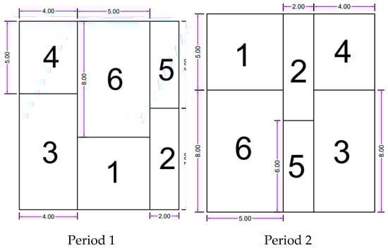
Figure 1.
Example illustration of the FBS-DFLP problem with unequal areas.
While solving the DFLP, it can be solved by creating new facility layouts in certain periods with an adaptive approach, assuming that the locations of the facilities will be easily changed. A solution can also be realized by creating a facility layout for all periods using a robust approach (RA), assuming that the locations of the facilities cannot be easily changed. Because DFLP is computationally complex, exact solution methods have difficulty finding a solution to large problems in a reasonable time. Therefore, Ant Colony Optimization (ACO) [3], Simulated Annealing (SA) [10], Genetic Algorithm (GA) [11], Particle Swarm Optimization (PSO) [12], etc., heuristic and meta-heuristic methods are used.
The motivation of the current study is to propose fast solution methods for the mathematical model, which has all the following features in the dynamic facility layout literature and was developed for the first time in the authors’ previous study [13]. The mathematical model’s characteristics are given as follows:
- Layouts with facilities that have different areas;
- Facilities whose shape can change with an aspect ratio;
- Layouts with FBSs;
- Assignment of different types of MHD;
- Considering the purchase, use, and non-use of MHD;
- Decisions on facility layouts are made simultaneously with decisions on material-handling vehicles.
Since the exact solution methods used in the problem structure discussed in this study have difficulty in producing solutions in a reasonable time, in this article, hybrid GA (HGA) and hybrid SA (HSA) algorithms are developed for FBS and DFLP with unequal areas (UA-DFLP) that simultaneously consider material handling decisions. In the proposed hybrid approaches, the Solving Constraint Integer Programs (SCIP) solver is used to obtain fitness functions for GA and SA separately. The main contribution of this study is to propose near-optimal and fast heuristic approaches for the integrated dynamic facility layout and material handling device assignment problem. Furthermore, a problem-specific chromosome structure and fitness value calculation approach based on a nonlinear mathematical model are proposed.
The remainder of the article is organized as follows: Section 2 describes the current literature review for the area; Section 3 explains the proposed methods, the problem description, solution coding, HGA steps, and HSA steps. Section 4 provides numerical experiments, findings, and subsequent analysis. Section 5 elucidates the conclusions drawn from these findings and outlines avenues for prospective research.
2. Background
In recent years, the DFLP has been widely studied in the facility layout literature, as the SFLP does not take into account the demand variability during the time horizon. Researchers have produced solutions using many methods for the DFLP, which is handled with different objectives and various facility layout structures. McKendall and Shang [3] for DFLP, which aims to minimize material handling and rearranging costs in general, obtained very effective results on two datasets from the literature using hybrid ant systems. Ulutas and Islier [5] tried to minimize the transportation and re-arrangement costs with clonal selection using real data. Kheirkhah and Bidgoli [14] developed game theory by taking into account the factor of being affected by competitive environments and found SA as the best model in game theory in which three different heuristics were modeled. Kumar and Singh [15] proposed a heuristic method to optimally solve the Dynamic Cellular Facility Layout Problem (DCFLP), which considers multiple products to be produced multiple times in the production order and provides optimal solutions in a reasonable time (these times change between 100 and 155,522 s according to problems) using similarity scores between facilities. In another study modeled with QAP, a mixed-integer nonlinear model was developed for a DCFLP with equal-area departments, considering not only transportation and rearrangement costs but also minimizing net electrical energy consumption. For model validation, twenty-five datasets corresponding to varying combinations of machines, time periods, and cells from the existing literature were utilized. A SA algorithm was used to solve the model [16]. Using the bacterial foraging approach and SA together, Turanoğlu and Akkaya [8] obtained satisfactory results on the most used test problems in the literature in reasonable calculation times that some of the range from under 1 to over 87,000 s. In another study, a Petri Net-based flexible manufacturing process model was developed for a DFLP solution, taking into account the total process cost. The proposed method combines the reachability graph algorithm and the search algorithm to achieve flexible production planning and dynamic layout schema [17]. Pournaderi et al. [18] have considered a multi-objective DFLP, which considers both the budget constraint and material handling equipment. A multi-objective Cloud Theory (CT) and TS were utilized to obtain solutions. The method parameters were determined using the Taguchi method and were tested by solving random samples. In the study by Molla et al. [19], the DFLP was solved using the Chemical Reaction Optimization (CRO) algorithm to optimize the total production cost economically. A new selection and repair operator was designed for the CRO, and the proposed algorithm was tested on a benchmark dataset. The results demonstrated that the proposed method yielded better outcomes in terms of cost minimization compared to other algorithms. There are studies in which computer-based methods are used for solving DFLP, and the solutions obtained are further improved. In one of these studies, the CRAFT method was used for DFLP, resulting in an 18.66% reduction in the total facility layout cost for a textile company [20].
Al Hawarneh et al. [21] developed a binary integer linear programming model (BILP) for the worksite layout problem by calculating the travel distances of workers and equipment with the site blocks algorithm, considering usability, overlap, installation, dismantling, forbidden zones, and relocation restrictions. With the developed model, the costs of transportation, dismantling, installation, and relocation of the facilities were minimized, resulting in a 20.68% reduction in the total settlement cost. Sahin et al. [22] modeled the classical single-row facility layout with mixed integer programming (MIP) by extending it to DFLP. The developed model is solved with hybrid methods where GA and SA are used with restart and acceptance probability strategies. The methods applied to 20 examples in the literature performed better in more than 60% of the problems, and the superiority of the hybrid SA method was robustly demonstrated. Matai and Singh [23] modeled DFLP linearly and obtained satisfactory results with little deviation (0.09%) on the two test problems. Hosseini et al. [24] proposed a novel mathematical model aimed at concurrently optimizing the placement of machines for each time period and orchestrating the logistics of transportation operations. To solve the model, they combined the modified genetic algorithm with the cloud-based SA algorithm. Guan et al. [25] investigated a dynamic expanded sequential facility layout (SFL) problem in which the relative positions and exact positions of the sections are calculated based on product processing. Constructing a mixed integer linear programming model for the problem, the authors proposed a hybrid evolution algorithm (HEA) combining binary swap and variation operations for the solution. HEA has achieved good results in comparison to the existing solutions and exact approximation (CPLEX) results of many samples. In the study of Palubeckis et al. [26], a variable neighborhood search (VNS) and a fast local search (LS) procedure were developed for the dynamic single-row facility layout problem. Computational experiments were performed on samples of up to 200 facilities and three or five planning periods to determine the effectiveness of the developed approach. The VNS heuristic was compared with the SA method, which is the most advanced algorithm for DFLP, and outperformed by a significant margin. In the study of Zouein and Kattan [27], an ACO algorithm was developed to solve the Dynamic Construction Site Layout Planning (DCSLP), and the performance of randomly generated datasets was measured. The results of the comparison with the examples in the literature showed that the algorithm achieved promising results. In the study of Pérez-Gosende et al. [28], a multi-objective mixed integer nonlinear programming model was developed for DFLP, which includes a bottom-up approach, contrary to the usual approach in the literature. The objectives of the developed model are to minimize the total material handling and total reorganization costs and to maximize the total closeness between facilities and the space utilization rate. The proposed model underwent application and validation through a case study conducted within the metal-mechanics industry, encompassing twelve facilities over a span of three periods, each lasting four months.
In their study aimed at minimizing transportation and relocation costs within a facility, Pourhassan and Raissi [29] extended the DFLP to minimize total combined rearrangement, material handling, and transportation costs by considering multiple carriers commonly used for transportation tasks between departments. To solve the developed model efficiently, two PSO-based and one GA-based hybrid algorithm were presented. The proposed hybrid PSO algorithms achieved better objective function values and solution times compared to the hybrid GA. In the study of Peron et al. [30], 3D mapping, indoor positioning systems, motion capture systems, and immersive reality technologies were introduced for the DFLP. The results show that these technologies provide a configurable facility layout as well as a structure that reduces costs in terms of sustainability, protects the environment, and improves social aspects [30]. According to Tayal et al. [31], the criteria used with unsupervised machine learning (UML) in the first stage for the DFLP were clustered, and the layouts were created with SA, chaotic SA (CSA), and hybrid (Firefly/CSA) methods. In the second stage, efficient/inefficient layouts were determined by data envelopment analysis (DEA), and in the last stage, the rankings of the layouts and efficiency scores were obtained with supervised machine learning (SML). This study obtained effective solutions for the problem with 12 facilities and 5 periods. A method with two main stages was proposed for the DFLP. In the first stage, layouts to be considered in each period were determined using a heuristic approach, forming the decomposition stages of periods in the dynamic programming (DP) approach. In the second stage, the DP model was solved using a hybridized genetic algorithm (GA) [32].
In the literature, studies dealing with UA-DFLP in accordance with real-world problems are increasing. Asl and Wong [12] used a modified PSO algorithm for UA-DFLP. Period swapping methods are used to avoid the model getting stuck in local optima. The developed method produced effective solutions to the problem examples in the literature. Liu et al. [33] proposed an approach with combining the Wang-Landau (WL) sampling algorithm and some heuristic strategies (blank point, push, and pressure strategies). The algorithm results tested on four groups of cases show that the proposed algorithm is effective. In another study, UA-DFLP modeled using the Quadratic Assignment Problem (QAP) was considered for the SDFLP. The problem was discussed using an example from the garment manufacturing industry, and a hybrid Firefly Algorithm (FA) and Chaotic Simulated Annealing (CSA) were employed to optimize the layout of the garment production unit. It was found that the proposed layout was superior to existing layout plans [34]. The SDFLP was examined in the context of disaster relief operations, and a mathematical model was developed for the problem by the same authors. Tabu Search (TS) and Chaotic TS methods were employed for solving the model. The developed approach was tested using datasets from the literature containing 12 departments and 5 periods, yielding effective results. The approach’s applicability for larger demand-based disasters was validated by increasing the number of departments to 30, and good results were obtained [35]. In another study involving facilities with unequal-area departments, a semi-robust cellular approach capable of handling continuous product mix and demand changes was modeled using multi-objective mathematical programming. In the proposed approach, instead of changing the facility layout, the locations of the cells’ pick-up/drop-off points are modified. The developed model can simultaneously determine the optimal number of cells and the intra-cell and inter-cell layout decisions. The model was solved using a modified NSGA-II that incorporates an advanced non-dominated sorting strategy and a modified dynamic crowding distance procedure [36]. An UA-DFLP solution developed for a construction site utilized information from Building Information Modeling (BIM) and a Geographic Information System (GIS) to dynamically optimize the site layout. The problem aimed to minimize the total on-site travel distance of personnel and equipment between facilities and to enhance the safety level of the construction site. A Guided Population Archive Whale Optimization Algorithm was applied. The results demonstrated that the total on-site travel distance was reduced by approximately 20% with the new arrangements [37]. In a recent study on unequal-area UA-DFLP, mathematical models for dynamic facility layout across several production planning periods were first developed. Secondly, a fixed-point movement strategy was proposed to solve the non-interference constraint handling problem based on the logistic relationship between facilities. The developed model was solved using a two-step method involving TS and a GA. A case study demonstrated the effectiveness of the proposed method [38].
UA-DFLP has been solved by modeling with FBSs in some studies. For Kulturel-Konak’s [39] regional-based DFLP, models were made in which facility sizes are decision variables and facilities are assigned to flexible regions with pre-configured positioning. In the model, facility locations, sizes, and entry/exit points are determined simultaneously, and a meta-heuristic method in which SA, VNS, and MIP are used together in the solution is used. Zha et al. [40] devised a hybrid (PSO and SA) algorithm within a fuzzy random environment to minimize the combined expenses related to material handling and reorganization, and the accuracy of the algorithm was ensured with the available test data. The developed algorithm was applied in a new aircraft assembly workshop facility layout planning, and the results were found to be effective in terms of both solution time (the run times change between 504 and 104,844 s) and solution quality. Erfani et al. [41] discussed the workshop scheduling problem with DFLP for a while and proposed a multi-objective Mixed-Integer Nonlinear Programming (MINLP) model. Considering the facility entry and exit points, proximity, and distance rating scores in the model, the authors reduced the average flow time of jobs by 10% in the model they solved using a hybrid method consisting of a LS and a GA. Hunagund et al. [42] considered UA-DFLP and FBSs together and obtained the optimum solution by using SA for the solution. Erik and Kuvvetli [13] developed MINLP for the use of UA-DFLP with FBSs and the combination with MHD assignment problems, showing that the integrated decision impacts the facility layout and leads to a reduction in overall costs. In the study of Zolfi and Jouzdani [43], in the multi-floor DFLP in which facilities with unequal areas are located, the number of elevators with FBS and the location of the elevator are taken into account as variables are modeled and solved by SA. With the developed method, eight test scenarios and some problems in the literature have been solved. The results demonstrated that the developed algorithm exhibits a superior capability in identifying optimal solutions compared to the algorithms under comparison.
Another important approach in the facility layout literature is the RA. In the RA, instead of creating new layouts repeatedly based on periods, a single settlement is obtained by considering all periods. Hosseini et al. [44] used a robust and simply structured hybrid technique based on imperialist competitive algorithms, variable neighborhood search, and SA algorithms to solve DFLP effectively. With the dataset from the literature, very good results were obtained regarding solution quality for most of the test problems of the hybrid algorithm. In some DFLPs, a robust structure is employed that accounts for changes across periods but develops a single facility layout for all periods. In one such study, a robust optimization model was proposed for a DFLP with unequal-area departments and uncertain demands, considering drop-off/pick-up points. Particle Swarm Optimization (PSO) was developed to solve the model, and the effectiveness of the approach was demonstrated using a real case from an assembly line [45].
Kaveh et al. [46] introduced chance-constrained programming and dependent chance programming, along with two hybrid intelligent algorithms for fuzzy programming and DFLP where the information flow is uncertain. These presented algorithms have been tested with some numerical examples, and their effectiveness has been demonstrated. According to Vitayasak et al. [6], they made layout arrangements to reduce transportation costs for DFLP with stochastic demand, but they observed that these regulations cause new costs and developed three different backtracking algorithms (BTA). By applying the developed methods to 11 problems in the literature, it was seen that the modified BTA obtained better results than the classical BTA and GA. Big Data Analytics (BDA) and a hybrid meta-heuristic for DFLP under stochastic demand. Firstly, the facility design factors were determined, and a number of reduced factors were obtained using BDA. Then, a weighted aggregate target for the problem is mathematically modeled, and a hybrid method consisting of Firefly and CSA is used to obtain the final facility layout. Peng et al. [11] developed a mathematical model that reveals a robust facility design for DFLP with uncertain material flow, and this model is solved by the GA. Samples of different sizes were solved with the developed GA and PSO, and it was seen that the robust layout performed well compared to the optimum layout for each period. In the study of Ghadirpour et al. [47], three MIP models were proposed for stochastic UA-DFLP, which takes into account routing flexibility, and large-scale problems in the literature were solved by GA and MIP methods. The results showed that the MIP models are valid for the problems and show competitive results. In another study, expert opinions were gathered for SDFLP from a sustainability perspective, and the diversity, velocity, and volume defined in big data were matched with the sustainability criteria of people, profit, and planet. The problem, expressed through a QAP-based mathematical model, had its efficiencies calculated using DEA. The ranking of the calculated efficiencies was performed using supervised machine learning. The objectives of the problem included minimizing material handling and rearrangement costs, hazards, and waste, and maximizing safety and aesthetics. To demonstrate which layouts best met these objectives, the k-means clustering method was applied, and the cluster that maximized the criteria (Cluster-3) was identified. Finally, energy consumption and CO2 emissions were calculated for each layout [48]. For a similar problem involving facilities with unequal departments and routing flexibility in SDFLP, three mixed-integer nonlinear programming models were proposed. In the models, independent demand random variables followed Poisson, Exponential, and Normal distributions. To validate the models, several small-scale test problems derived from a real case in the literature were solved, and large-scale test problems were solved using a GA within a reasonable computation time [49]. In the study of Khajemahalle et al. [10], the creation of a robust counterpart of the facility layout for a DFLP in which the material flow between facilities and re-arrangement costs are uncertain is achieved by a hybrid method consisting of Nested Sections and SA algorithm. The results showed that the created hybrid algorithm is very effective in achieving good solutions with less computational effort. Hunagund et al. [42] developed a mathematical model that provides a robust layout design for UA-DFLP with FBS. The developed model was adapted to the SA algorithm and aimed to minimize a penalty cost function. Zhun et al. [50] developed a multi-objective pigeon-inspired optimization algorithm for DFLP to optimize cost and space utilization, taking into account uncertain product demands. Using a global collaboration mechanism to balance local and global search, the authors demonstrated the validity of the approach with an industrial case and revealed that the algorithm developed for the proposed problem performed better. Alamiparvin et al. [51] formulated the stochastic DFLP (SDFLP) with facilities with unequal area by considering upper bounds. Examples of problems where product demand is normally distributed with a known expected value and variance are solved by P9. The effectiveness and validity of the developed PSO have been verified. Esmikhani et al. [52] proposed a SA and Modified Non-Dominant Sequence Genetic Algorithm II (MNSGA-II) to solve the DFLP problem where flows between facilities consist of random fuzzy numbers and it is forbidden to place facilities in some areas of the layout. It has been determined that the SA algorithm finds better solutions with the material handling cost of the operators and cranes, and the MNSGA-II algorithm finds better solutions with the usability of the cranes in the problem, which aims to minimize the material handling costs of the operators and cranes and to maximize the usability of the cranes. The characteristics, objectives, solution methods, and types of problems addressed in recent studies on DFLP are summarized in Table 1.

Table 1.
Studies for the dynamic facility layout problem.
When examining Table 1, it becomes evident that numerous authors approach the DFLP in various ways. The existing literature exhibits diversity concerning facility structures (equal, unequal, flexible, fixed), objectives, placement configurations within the facility (bay, slicing, etc.), solution methods, and problem types (stochastic, deterministic, cellular, etc.). In this study, two effective hybrid methods (SCIP solver is collaborated with GA and SA) were developed for a novel problem previously introduced to the literature by Erik and Kuvvetli [13]. The effectiveness of the proposed methods is demonstrated through problem examples with known exact results. Furthermore, the PSO method developed by Pourhassan and Raissi [29] was adapted to the problem under consideration and compared with the methods proposed in this study. The results substantiate the effectiveness of the proposed methods.
3. Materials and Methods
For the DFLP, different methods are used together in many studies [6,8,10,22,39,58]. Due to the NP-Hard nature of the problem, the literature has increasingly gravitated towards heuristic or hybrid solutions. In this study, two hybrid meta-heuristic methods have been developed in which a GA and an SA with the SCIP solver that offers deterministic solutions are used together. The methods of the study are explained in Section 3.1, Section 3.2, Section 3.3 and Section 3.4.
3.1. The Mathematical Model Used for the Problem
The MINLP model is shown below, developed by Erik and Kuvvetli [13] for the problem addressed in this paper. This model was utilized in conjunction with the GA and SA algorithms to develop the HGA and HSA methods.
Objective function:
Constraints:
The objective function in Equation (1) aims to minimize costs. Equation (2) represents material handling costs between departments; Equation (3) represents rearrangement costs; and Equation (4) represents purchase costs of transportation vehicles and costs associated with the use and non-use of these vehicles.
Equations (5)–(8) calculate the horizontal and vertical distances for material handling between departments and the rearrangement-induced distances. Equation (9) ensures each department is assigned to a single cell. Equations (10) and (11) calculate the width of each cell based on the departments assigned to it. Equations (12) and (13) determine the horizontal positions of the department centroids. These equations, along with Equation (14), ensure departments remain within the facility’s boundaries along the horizontal axis. Equations (14)–(21) determine the vertical positions of the department centroids and prevent vertical overlap. Equation (22) ensures departments stay within the facility’s vertical boundaries. Equations (23)–(28) maintain the same dimensions and centroid coordinates for departments across consecutive periods if no rearrangement occurs. Equation (29) ensures the total time a vehicle spends handling materials is less than its available time during the planning horizon, also determining the required number of vehicles. Equations (30)–(32) describe the relationship between the number of required vehicles of type g, the number of purchased vehicles, and the number of redundant vehicles in period t. Equation (33) ensures transportation between departments i and j in period t is handled by a vehicle of type g. Finally, Equations (34) and (35) specify the constraints on the variables used in the model.
3.2. Outline of the Proposed Hybrid Heuristics
In this study, two heuristics are proposed that combine the SCIP solver with a GA and an SA. In the HGA, genetic algorithm parameters, genes, and chromosomes are determined. Then, a random initial population of these chromosomes is generated. The fitness values of each individual are calculated using a MINLP model via the SCIP solver. The outline of the HGA is depicted in Figure 2. The basic idea behind the methodology is to find a solution by checking the feasibility of the main DFLP. Therefore, in the algorithm, chromosomes created in the GA determine a random location within the layout and enter the model as a parameter. Under the constraints of the MINLP model, the fitness functions are calculated and fed to the genetic algorithm individual. In the proposed algorithm, the fitness value of the solutions that are not feasible is penalized with a huge number, and the probability of survival is decreased for infeasible solutions.
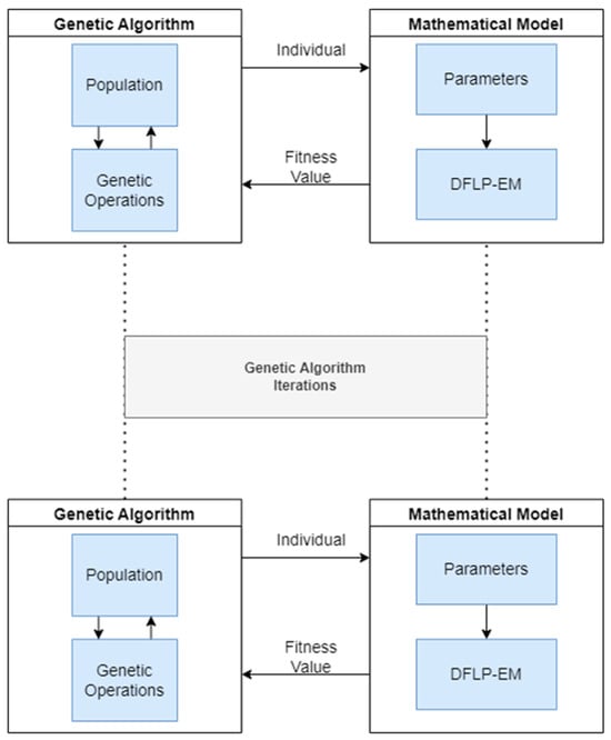
Figure 2.
Outline of the HGA.
The HSA has fewer steps than the HGA. In this approach, SA algorithm parameters are determined. Then it is created an initial solution and calculated fitness value from the MINLP model via the SCIP solver. Lastly, it creates new neighbor solutions to find better results until reaching the stopping criterion. The outline of the HSA is depicted in Figure 3. The basic idea behind the methodology is to search for neighboring solutions by checking the feasibility of the main DFLP. Therefore, in the algorithm, new random locations are created with a formula that uses the neighbor coefficient. Under the constraints of the MINLP model, the fitness functions are calculated and fed to the HSA.
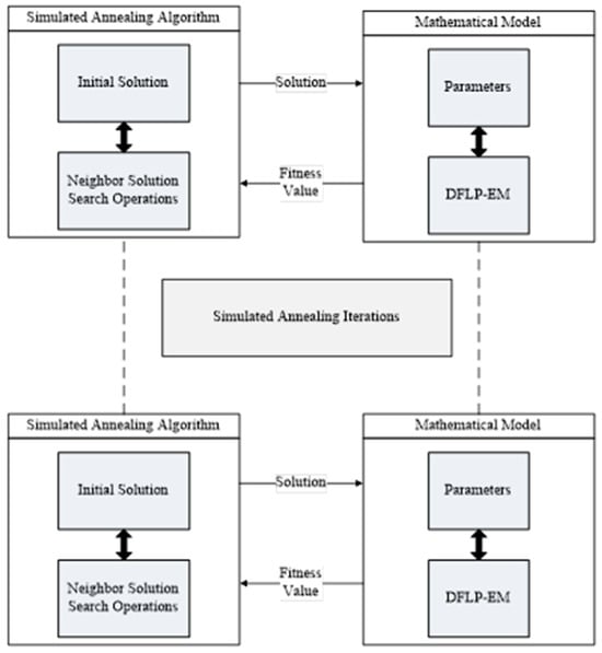
Figure 3.
Outline of the HSA.
3.3. Genetic Algorithm
The GA is a population-based algorithm originating from the theory of evolution [6,60,61]. The GA is a search and optimization method that uses evolutionary methods in nature [62]. With this algorithm, the survival and reproduction probability of an individual is determined according to its suitability by applying natural selection [63]. The GA has demonstrated successful applications in diverse areas, including function optimization, scheduling, machine learning, design, and cellular manufacturing. The GA scans a part of the solution space, not the whole. With an effective search, a solution is reached in a much shorter time [64].
The GA operates with populations of chromosomes, each representing a coded solution to the problem at hand. These chromosomes are composed of fundamental units referred to as basic cells. Within each chromosome, a fitness value is assigned to gauge its success rate. Typically, an initial population is randomly generated, and through an iterative evolution process, fitness selection is conducted using crossover and mutation operators to generate a new population [4]. Offspring are produced by crossover and mutation processes on randomly selected chromosomes from the population. The suitability of these chromosomes determines their survival probability [6].
The stage of applying a GA to a problem begins with creating the gene and the chromosome structure formed by these genes. While the generated gene carries the basic information, the chromosome constitutes the solution consisting of these genes and is called the individual. The combination of many chromosomes forms a population. At this juncture, the user determines the population size to regulate its magnitude. Subsequently, solutions are evaluated, and the fitness function of the problem is determined. The GA usually starts with a randomly generated initial population. Then, the fitness function values of all chromosomes in the initial population are calculated. Thanks to these values, the elitism process can be operated in which good individuals can survive better than the others. After the initial population is created, individuals are crossed to produce better individuals. In order to ensure diversity in individuals, the mutation is applied to individuals at the determined mutation rate. Finally, the extinction process is handled to survive only the pre-determined population size. According to the determined stopping criterion, crossover operation, mutation operation, and elimination operation are applied. In this way, the initial population is gradually improved [65]. The algorithm tries to obtain the best solution in the end by preserving the individual with the best fitness value at each stage. A flowchart of the genetic algorithm is shown in Figure 4.
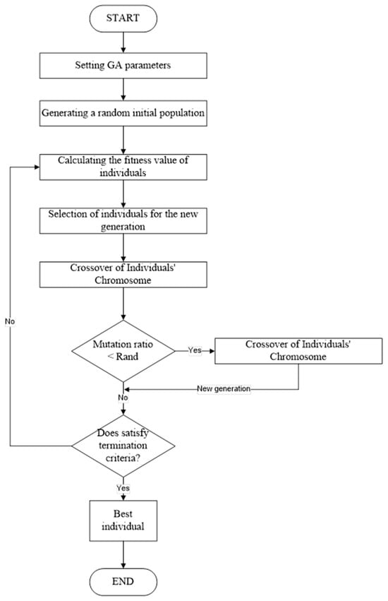
Figure 4.
Genetic algorithm procedure.
3.3.1. Individual Representation
The nature of the problem should be taken into account when generating the gene in HGA. The genes in the HGA are formed according to the period (T) and the number of facilities (N). The flexible division structure consists of randomly generated numbers between 1 and B + 1, with B being the maximum number of divisions. The integer part of the randomly generated numbers shows which partitions the facilities are assigned to, while the decimal part shows the placements of the facilities in the same bay, with the smaller one taking precedence. While the divisions are numbered from left to right (x = 0.00), facilities are ordered from bottom to top (y = 0.00). An example chromosome and its facility location are given in Figure 5.
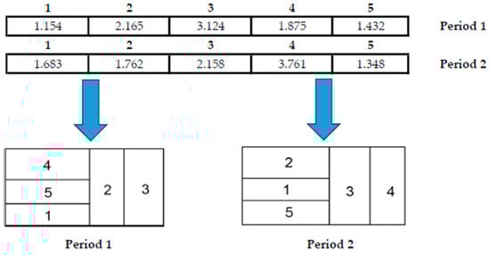
Figure 5.
An example chromosome representation and layout plan for FBS-DFLP-2.
3.3.2. Evaluation of an Individual
Mixed integer programming (MIP), one of the most frequently used methods in facility layout problems, is a deterministic method with optimum results. MIP has also been widely used in DFLPs [4,7,9,13,22,23,41,46,56,57,59]. In this study, the model developed by Erik and Kuvvetli [13], which deals with the combined DFLP and assignment of MHD, was used. The model, which tries to create the optimum facility layout in different periods, tends to minimize the sum of material transportation costs, re-arrangement costs, and the costs of using, not using, and purchasing MHD. A FBS is used when assigning facilities with different areas on a continuous facility area.
In the evaluation of the solutions of the proposed method, the fitness value of an individual is obtained by the optimal solution of the DFLP with FBS and material handling systems assignment model (DFLP-EM). The evaluation procedure is given in Algorithm 1.
| Algorithm 1: DFLP-EM fitness evaluation |
| Procedure DFLP-EM (chromosome, |
| , ) |
| Generate facility layout (S0) from chromosome |
| Generate , , from S0 |
| Z0 = Evaluation (,, , ) // run DFLP-EM model |
| If Z0 feasible then |
Sg S0 S0 |
| Zg Z0 |
| else |
| Sg |
| Zg M |
| end if |
| Return Sg, Zg |
| End Procedure |
During the HGA, a chromosome represents the randomly generated facility layouts, and the , , and variables are fed as parameters to the mathematical model used in Erik and Kuvvetli [13]. A solution (S0 or Sg) includes decision variables, which are , , , . The objective function (Z0 or Zg) can be calculated by Equations (1)–(4) using the decision variables of the solution. Where is related to classical facility layout costs, occurred from the change in facility layout during periods, and includes the MHD-related costs.
The MINLP that is used for computing the fitness function is to ensure the feasibility of solutions through a set of constraints. These constraints encompass several aspects, including the allocation of only one flexible bay to each facility, the calculation of flexible bay widths based on assigned facilities and aspect ratios, the requirement for facilities to remain within the layout and flexible bay boundaries, the computation of horizontal and vertical centers of facilities within the facility, the prohibition of facility overlap, and the stipulation that facilities, if not rearranged, must maintain consistent dimensions and coordinate centers. Furthermore, constraints include ensuring that the transportation vehicles utilized adhere to planning horizons in terms of their capacity, loading and unloading times, and speeds. It is also important that there are no unused transportation vehicles if a new material handling vehicle is acquired. Lastly, the constraints dictate that material handling between facilities should be facilitated by a specific type of vehicle.
3.3.3. Selection Method
The Roulette Wheel (RW) method was used as the selection method in the study. The RW method performs a normalization by dividing the fitness values calculated for each chromosome created by the sum of the fitness values of all chromosomes [66]. It then decides whether the chromosome will die or live according to the random numbers generated. RW is a method that works with the logic of maximization, but the purpose of the fitness value calculated in the problem is to provide the minimum cost. Therefore, the RW method is applied by making the following transformation for the fitness value.
where is the fitness value; is the arc length; is the survival probability of the individual; and R is the initial population size.
After the calculations made with Equations (36) and (37), individuals who are strong survive with a high probability. The surviving chromosomes move on to the next step, crossover. At the same time, there is a small probability that non-feasible solutions will survive the transformation. This ensures diversification and reduces the probability of getting stuck in local minimums.
3.3.4. Crossover Process
Crossover is the process of generating new solutions (children) from two main solutions (parents). The reproductive process creates clones of good individuals but not new individuals [67]. The crossover function is applied to individuals in the hope of producing better individuals. An example of crossover for the FBS-DFLP with MHD assignment problem is given in Figure 6.
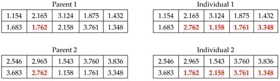
Figure 6.
An example crossover operation.
The crossover process starts with the selection of the pairs to be crossed first. In the new individual pool formed, individuals are randomly matched, and pairs are formed for crossover. In order to make the crossover decisions of the selected pairs, randomly distributed random numbers between 0 and 1 are generated. If these generated numbers are less than the crossover probability (Pc) determined for crossover, the crossover occurs. In the proposed algorithm, a random gene is selected for the one-point crossover mechanism, and the genes further from this point are exchanged between individuals.
3.3.5. Mutation Process
Mutation introduces novel genetic structures into the population by randomly altering certain genes. This process aids in avoiding local minima and promoting diversity within the population [68].
In the proposed algorithm, a mutation probability (Pm) determined by generating a random number between 0 and 1 for each gene (T*N) is compared with (usually between 0.001 and 0.01). The mutation process is applied to genes with random numbers lower than the determined mutation probability. The mutation process used in this study is shown in Equation (38):
where and are the individuals before and after mutation, l and u are the lower and upper bounds of the genes, and k are neighborhood (0.01–0.1) and a random number between −1 and 1, respectively.
3.4. The Simulated Annealing Algorithm
SA is a random search method proposed by Kirkpatrick et al. [69] to solve optimization problems. It has been successfully applied to many large-scale real-life problems. Due to its ease of implementation, convergence, and strategy to avoid local optima, SA has become a common method for solving optimization problems [70]. SA gets its name from the similarity with the physical annealing process of solids [71]. SA is a step-by-step improvement method. During this process, not only better results are accepted, but also, with a certain probability, bad solutions. This ensures that the algorithm gets rid of the local bests. This process is one of the main features of SA. In SA, the goal is to get rid of the local best and reach the general best. The probability of acceptance is expressed in based on a conceptual temperature. Here, expresses the change between the objective functions of the current solution and the generated neighbor solution. T is the temperature, which is the control parameter [54].
For small values of , the probability of accepting the bad solution is higher than for large values. Also, most of the new solutions produced at high temperature values will be accepted.
As the temperature tends towards zero, the likelihood of accepting new solutions diminishes [55]. Therefore, in the SA algorithm, the initial temperature is generally set as a high value to avoid local optima. Despite its easy applicability and good-quality solutions for combinatorial optimization problems, the disadvantages of SA are that it requires more computer time and requires a lot of experimentation for parameter selection [45].
Before applying SA to DFLP, some definitions must be made. In this study, the solution to the problem is represented as a two-dimensional matrix. The rows of the matrix correspond to the periods, while the columns correspond to the facilities. The elements of the matrix show the bay where the facilities are located and their positions in the bay. An equation with a neighborhood coefficient parameter is used to obtain the neighboring solution from the current solution. With the created equation, the randomly generated numbers for the facility locations are added or subtracted. The addition or subtraction process changes randomly depending on whether the number obtained at the end of the equation is produced as positive or negative. The Annealing Chart is a structure of parameters used in SA. It includes the parameters of initial temperature (), neighborhood coefficient (), cooling rate (), final temperature (), acceptance criterion, and finishing condition. The initial solution is randomly generated by the algorithm in this study. The initial temperature must be large enough for the majority of solutions generated at the beginning of the algorithm to be accepted. As a result of the experiments carried out in this study, different initial temperatures were determined for different instances. Cooling should be carried out slowly to obtain good-quality solutions. A cooling rate is used for this. When moving from one temperature to another, the previous temperature is multiplied by the cooling rate to find the new temperature (). Parameter selection is an important issue for all heuristic optimization problems. In SA, the cooling rate is an important parameter and has a great influence on achieving good results. Therefore, in this study, the best cooling rate options were determined by conducting experiments for cooling rates. The final temperature was also used as the stopping condition for the algorithm. The search ends when the algorithm reaches the final temperature.
3.4.1. Solution Encoding in the HSA
The solution encoding scheme used for the HSA is the same as the individual representation in Section 3.3.1. Here, as in the previous one, random numbers are generated, not exceeding the number of bays, and the integer part of the number indicates the bay to which the facility is assigned, and the decimal part indicates the location of the facility in the bay. The rules for facility layout representation remain unchanged. In other words, if the decimal part of the number produced for the facility is smaller, the priority belongs to that facility. While the divisions are numbered from left to right (x = 0.00), facilities are ordered from bottom to top (y = 0.00). According to these rules, an example representation of the facility layout is given in Figure 5.
3.4.2. Evaluation of a Solution
In order to evaluate the solutions in HSA, as in HGA, the model developed by Erik and Kuvvetli [13], which deals with the combined DFLP and assignment of MHD, was used. In the evaluation of the solutions of the proposed method, the fitness value of an individual is obtained by the optimal solution of the DFLP-EM. The evaluation procedure (Algorithm 1) also applies to the evaluation of the HSA. The only difference here for HSA is that the facility layout is not derived from chromosomes. There is a random facility layout produced in HSA, and different solutions are sought with the neighborhood move operation.
3.4.3. Neighborhood Structure
In the proposed study, the transition from one configuration to another involves selecting specific periods (rows) and subsequently implementing the insert operation on the chosen periods.
denotes the ith element of the solution after the insert operation, while denotes the ith element of the solution; l and k are the lower and upper bounds. Finally, denotes the neighborhood coefficient, and k is a random number between −1 and +1.
The formulation shown in Equation (39) is used to perform the insert operation. To calculate the amount of change in Equation (39), the maximum number of bays is multiplied by the neighborhood coefficient and divided by 2. The final amount of change is calculated by multiplying the obtained number by a random number between −1 and 1. Thus, the amount of change to be obtained will be able to function both as addition and subtraction. When this process is repeated many times, it is possible for some elements to exceed the maximum number of bays or decrease below the minimum number of bays. In order to prevent this, elements that are not between the minimum and maximum values determined immediately after the operation are replaced with a random number generated between these values.
4. Results
The results obtained from the study are presented in this section. First, it was determined how to set the user-defined parameters. Thus, the ideal user-defined parameters to be used by the HGA and HSA methods are found as provided in Section 4.1. In order to test the proposed methods, the problems called FBS-DFLP-1, 2, 3, and 4 in the study of Erik and Kuvvetli [13] were solved. These problem instances represent problems involving rectangular facilities with FBS, unequal areas, and a certain aspect ratio. In addition, the necessary MHD and their assignments are also included in the problem, as aforementioned. These problem instances are solved by HGA, HSA and PSO methods known in the literature and results were presented in Section 4.2. Results for more complex problem instances are given in Section 4.3. Finally, sensitivity analysis is performed and summarized in Section 4.4.
4.1. Parameter Tunning
The user-defined parameters of the HGA and HSA should be tuned in order to find better generalization ability of the algorithms. The HGA algorithm includes while the HSA algorithm includes and parameters to be set. The depends on the problem instance; therefore, they are neglected. For instance, in the FBS-DFLP-2 problem instance, and . In order to obtain parameters ( and ) of the HGA and HSA, each parameter was run separately with the computer program developed for hybrid algorithms. These parameters were determined by taking into account the fitness values of the instance. In Figure 7, the values of the fitness function according to various initial population size, number of iterations, crossover probability, neighborhood coefficient, and mutation probability values are shown for the proposed HGA algorithm. In Figure 8, the values of the fitness function according to various the initial temperature, the final temperature, coefficient neighborhood, and cooling rate are shown for the proposed HSA algorithm.
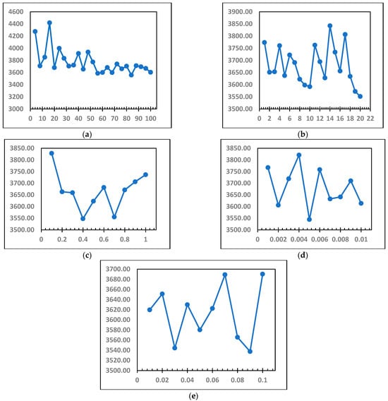
Figure 7.
Fitness values of the proposed HGA algorithm according to different user-defined parameters for the FBS-DFLP-2. (a) Initial population size/fitness value. (b) Number of iterations/fitness values. (c) Possibility of crossover/fitness value. (d) Neighborhood coefficient/fitness value. (e) Possibility of mutation/fitness value.
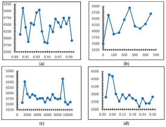
Figure 8.
Fitness values of the proposed HSA algorithm according to different user-defined parameters for the FBS-DFLP-2. (a) Cooling rate/fitness value. (b) Final temperature/fitness value. (c) Initial temperature/fitness value. (d) Neighborhood coefficient/fitness value.
When the fitness values obtained by keeping the other parameters constant are examined, the initial solution size () was 84, while the minimum cost was reached. The initial solution size has been updated to 84. While the initial solution size is 84 and other parameters are fixed, the number of iterations (/terminate criterion) is tried and the number 20 is reached. A 2% difference was found between the optimum solution and the fitness function value found by the genetic algorithm. The crossover probability () specifies the condition for crossing strong individuals produced by reproduction. After updating the iteration and initial solution size, the crossover probabilities were tried, and the value of 0.4 was found. In the determined formula used for the mutation process, the neighborhood coefficient directly affects the number to be added or subtracted. In the algorithm operated by keeping other parameters constant, the neighborhood coefficient () value of 0.09 and the best fitness value were obtained. The mutation must be performed so that the crossed individuals are not caught in the local minimum and the solutions are diversified. While determining the mutation probability (), which is the prerequisite in the mutation process, the algorithm was run with the updated parameters, and the best fitness value of 0.005 was reached.
Similar to the HGA results, the cooling rate (sk) is 0.95 for achieving the minimum cost. While the cooling rate is 0.95 and other parameters are fixed, the coefficient of the neighborhood is tried and set as 0.22. There is a 2.38% difference between the optimum solution and the HSA’s fitness function value. After updating the cooling rate and the co, the initial and final temperature are set as 1000 and 0, respectively. There have been obtained solutions with a 0.69% difference from the optimum value for the FBS-DFLP-1 instance and just a 0.01% difference from the optimum value for the FBS-DFLP-2 instance using these parameters. There have been obtained solutions with a 0.69% difference from the optimum value for the FBS-DFLP-1 instance and just a 0.01% difference from the optimum value for the FBS-DFLP-2 instance using these parameters. However, these parameters did not provide good results for the FBS-DFLP-3 and FBS-DFLP-4 instances. For this reason, the parameter tuning repeated for these instances. The values of 0.995, 2, 25000, and 0 were reached for the cooling rate, neighborhood coefficient, initial temperature, and final temperature, respectively. With these new parameters, optimum results were obtained for FBS-DFLP-3 and FBS-DFLP-4 instances.
4.2. Results for Known Instances
Contrary to mathematical modeling, meta-heuristic algorithms search for solution spaces randomly, so the results can vary from run to run. Therefore, the developed HGA and HSA methods were run 10 times for each problem instance. Additionally, to demonstrate the effectiveness of the proposed methods, the PSO method developed by Pourhassan and Raissi [29] was adapted to problem instances that are known optimal solutions. Performance criteria including minimum cost (fitnessc function), average cost, maximum cost, standard deviation of cost, and average speed were chosen for the simulations. In assessing the algorithms’ performance and quality, these criteria were computed for each algorithm, given the significance of cost, standard deviation, and speed. All computations were conducted using a personal computer equipped with an Intel Core i5-10200H CPU operating at 2.40 GHz, running a 64-bit Windows 10 operating system with 16 GB RAM, and utilizing the MATLAB coding platform.
Solutions were obtained for four test problem instances known in the literature. The first instance has four departments and three periods, while the second instance has five departments and two periods. The other two instances are relatively more complex problem instances; the third one has eight departments and six periods, while the last one has 12 departments and four periods.
4.2.1. Results for the FBS-DFLP-1 Instance
The FBS-DFLP-1 problem instance has four facilities with unequal areas and three periods. The optimum value of material handling, rearrangement, purchasing a handling device, and using and disusing costs in the problem involving handling device assignment and FBS was found to be 4454.95 TL.
Figure 9 shows the PSO, HGA, and HSA results for the FBS-DFLP-1 instance during the different runs. The cost deviates by 13.55%, 2.34%, and 2.97% on average for the PSO, HGA, and HSA solutions obtained in the study. No difference was found from the optimal solution in the use cases and assignments of transport vehicles. There was found an 8.92%, 0.22%, and 0.69% difference between the best solution and optimum value for the PSO, HGA, and HSA methods, respectively.
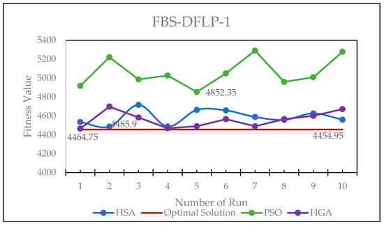
Figure 9.
Fitness changes for FBS-DFLP-1 during runs.
When the study that obtains the optimum results and that study are compared, it is seen that different facility layouts are formed. Figure 10 shows layouts closest to the optimum cost of the FBS-DFLP-1 instance within the scope of this study.
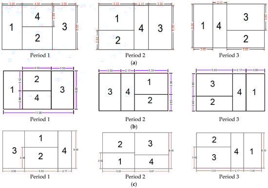
Figure 10.
The best layout obtained from the HGA and HSA for the FBS-DFLP-1. (a) The best layout obtained from the HGA; (b) the best layout obtained from the has; (c) the best layout obtained from the PSO.
4.2.2. Results for the FBS-DFLP-2 Instance
The FBS-DFLP-2 problem instance consists of five facilities with different areas and two periods. The PSO, HGA, and HSA reached the results with an average of 19.18%, 3.91%, and 5.37% deviation from the optimum cost (3488.71 TL), respectively. Figure 11 shows the results for run-to-run of the PSO, HGA, and HSA.
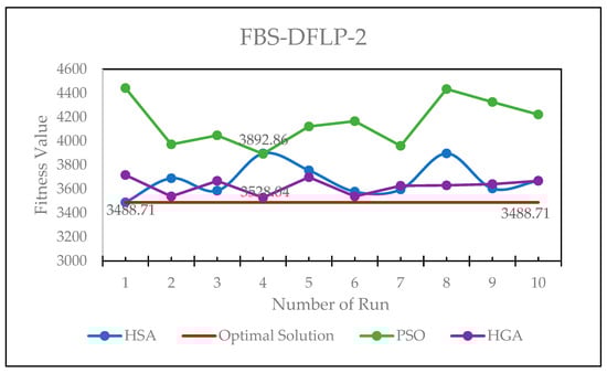
Figure 11.
Fitness changes for FBS-DFLP-2 during runs.
According to the material handling device decisions obtained from the proposed methodologies and the optimal solution, both proposed methods have the same material handling assignments as the optimal solution. The fitness function value of the best settlement found with the PSO, HGA, and HSA deviated from the optimum cost by 11.58%, 1.13%, and 0.01%, respectively. The best layout obtained from the proposed methodology is shown in Figure 12 for the HGA, HSA, and PSO methods.
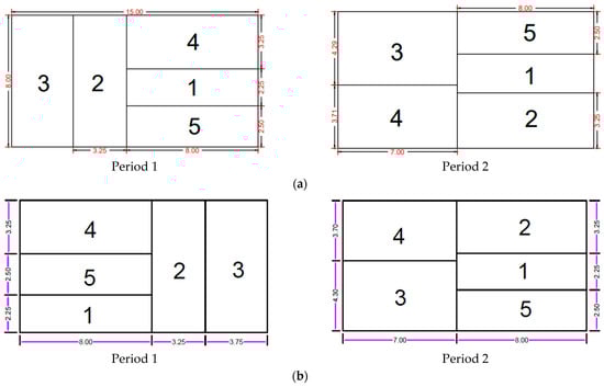
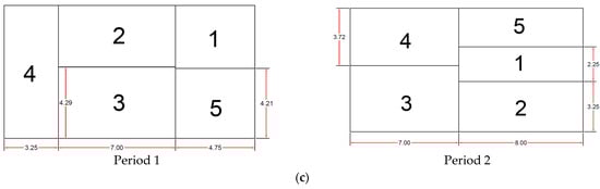
Figure 12.
The best layout obtained from the HGA and the HSA for the FBS-DFLP-2. (a) The best layout obtained from the HGA; (b) the best layout obtained from the HSA; (c) the best layout obtained from the PSO.
4.2.3. Results for the FBS-DFLP-3 Instance
The FBS-DFLP-3 problem instance consists of eight facilities with unequal areas and six periods. Figure 13 indicates that the PSO, HGA, and HSA solve the instance with an average of 10.38%, 4.75%, and 2.41% deviation from the optimum cost, respectively (38431.21 TL).
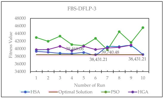
Figure 13.
Fitness changes for FBS-DFLP-3 during runs.
The fitness function value of the best settlement found with the PSO, HGA, and HSA deviated by 3.41%, 2.70%, and 0.00% from the optimum cost, respectively. Layouts obtained from the HGA, HSA, and PSO are shown in Figure 14. In the results obtained, there are different uses and assignments related to transportation vehicles. While five vehicles were purchased from a vehicle type in the optimum solution, six vehicles were purchased from two different vehicle types in the best solution found in the HGA, and one vehicle was out of use in the fourth period.
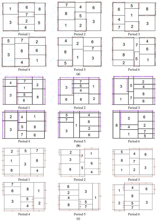
Figure 14.
The best layout obtained from the HGA and the HSA for the FBS-DFLP-3. (a) The best layout obtained from the HGA; (b) the best layout obtained from the HSA; (c) the best layout obtained from the PSO.
4.2.4. Results for the FBS-DFLP-4 Instance
The FBS-DFLP-4 problem consists of 12 facilities with different areas and four periods. The PSO, HGA, and HSA achieved the results with an average of 4.20%, 2.41%, and 1.02% deviation from the optimum cost (72,594.23 TL), respectively. The results of the FBS-DFLP-4 instance can be seen in Figure 15.
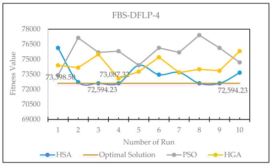
Figure 15.
Fitness changes for FBS-DFLP-4 during runs.
The best layout found in the PSO, HGA, and HSA deviated 1.11%, 0.68%, and 0.00% from the cost, respectively. These layouts are shown in Figure 16. The solution of the HGA obtained in the assignment of transport vehicles is the same as the optimum solution in the first period, and 11 units of one type of vehicle are purchased and used. However, there is a vehicle out of use in the second period and two vehicles purchased in the fourth period.
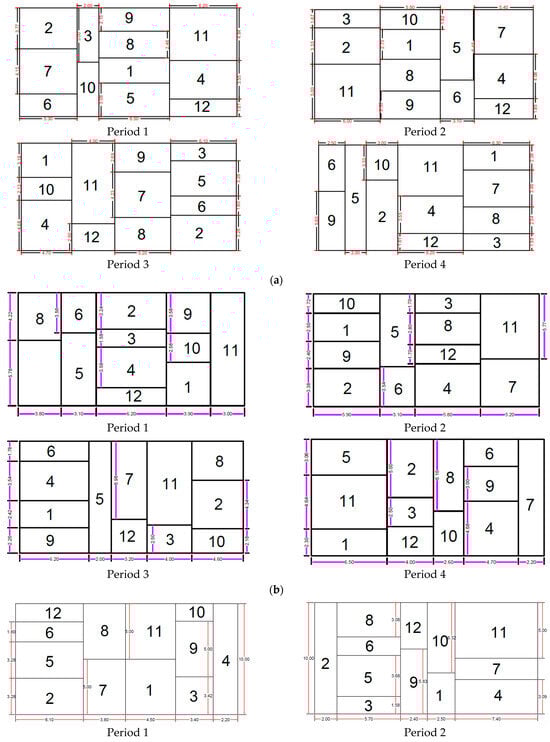
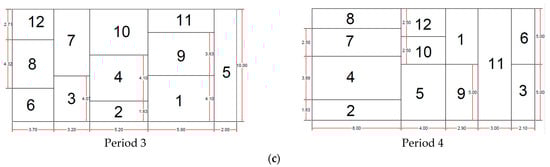
Figure 16.
The best layout obtained from the HGA and the HSA for the FBS-DFLP-4 (a) The best layout obtained from the HGA; (b) the best layout obtained from the has; (c) the best layout obtained from the PSO.
4.2.5. Evaluation of Results
The discrepancies, means, and average CPU time for four problem instances solved using the HGA, HSA, and PSO are presented in Table 2. Upon analysis of the results, it is evident that the HGA has achieved solutions with deviations of less than 1% for two problem instances and below 3% for the remaining two instances. The HSA has reached the optimum solution for three instances, and it found a solution for the other instance as a %0.69 difference. The results of the PSO method adapted to the problem are behind the HGA and HSA methods. Among the four solved problems, the closest solution found by PSO is for FBS-DFLP-4 with 1.11%. The solutions for other problems are over 3%. Although the maximum and minimum deviations of the solutions found are at reasonable levels, it can be concluded that the results are achieved with low variability. There has been a great improvement in the solution times of the problem, and the solution times, which exceed one day, have decreased to less than 10 min for the HGA method. The HSA method has provided better resolution time than the HGA.
Table 2.
Performance of algorithms for problem instances.
4.3. Computational Study
Hybrid meta-heuristic methods have shown excellent performance in solving problems with known optimum solutions. In addition to known problems, more complex problem instances have also been investigated to determine the performance of these methods in solving more intricate problems. The general characteristics of the examined problem instances are provided in Table 3. In the newly considered problem instances, the number of facilities ranges from 8 to 24, the average of facilities’ maximum aspect ratio ranges from 4 to 16, and the average of facility areas ranges from 7.5 to 19.55 m2. There are a maximum of 5 periods and 10 flexible bays. Similar to previous problems, two different types of vehicles are used in these problem instances.
Table 3.
Characteristics of problem instances.
The results of the costs and solution times for each problem considered are presented in Table 4. According to these results, the HSA algorithm has consistently outperformed in solving all the problems. In terms of total cost, the HSA algorithm has been observed to yield better solutions by an average rate of 2.73% when compared to the HGA algorithm. In the most significant difference, the HSA algorithm achieved a notably better result for P13 compared to the HGA algorithm, with an 8.30% difference. When the developed algorithms are compared in terms of solution times, the HSA algorithm once again exhibits a clear advantage. It achieves better solutions in an average of 122.82% less time, and in the most extreme case, it obtains solutions nearly four times faster with a 381.99% difference compared to the HGA algorithm. The HGA algorithm managed to achieve faster solutions in only 3 out of the 22 problem instances, but in those cases, it incurred 5.50%, 0.09%, and 8.30% higher costs for the solutions. Table 4 also presents the results of the PSO algorithm developed by Pourhassan and Raissi [29] and adapted to the problem. According to these results, the HSA outperformed the PSO algorithm across all problem instances, yielding superior solutions. The HGA achieved worse results than the PSO algorithm in only six instances. Similar trends were observed in terms of computational time. These findings indicate that the proposed methods obtain more effective results in a more reasonable time frame compared to the PSO algorithm.
Table 4.
Cost and solution time results for problem instances.
In addition to the results of the obtained costs and solution times, other factors, such as the total facility rearrangement distance, the total material transport distance within the layout, and the number of MHD used, have also proven to be significant when evaluating the effectiveness of the algorithms. These results are presented in Table 5. A detailed evaluation of the algorithm solutions reveals that, as expected, the HSA algorithm achieves lower costs by rearranging facilities more in most of the problems. However, an intriguing result is that the HGA algorithm performs more transportation in terms of the total facility rearrangements. This situation implies that, despite the transportation conducted by the HGA algorithm, it fails to reach transportation routes with shorter distances or lower costs. This is evident in the HGA algorithm having a total material handling distance of 2840.19 m greater. When examining the preferences for MHD, it is observed that both algorithms require the same type and the same number of handling devices. Furthermore, as problem complexity increases, the algorithms make different choices regarding the types of handling devices. This indicates the influence of handling device decisions in conjunction with facility layout decisions.
Table 5.
The change in some variables (rearrangement, movement, and MHD number) according to the solution algorithms.
4.4. Sensitivity Analysis
To investigate how the variation of parameters affects the solution in the developed HGA and HSA, solutions were obtained for the P1 instance by varying the parameters by ±10%, as shown in Table 6. Material flows between departments are excluded from the sensitivity analysis as these flows directly affect the facility layout. In the sensitivity analysis conducted, the effects of these parameters on decision variables (changes in layout), objective function value, and solution time were measured. In some instances, the change in the parameter caused infeasible solutions; therefore, these instances were labeled as INF. For the HGA method (Table 6), reducing the facility width and height resulted in infeasible solutions, as departments could not fit within the facility. A similar situation was observed when department areas were increased. This shows us that the width, height, areas, and number of bays are the most important parameters for achieving solutions for the layout problem. When analyzing how the quality and CPU time of the solution change with changes in these parameters, it is seen that the objectives of both algorithms deviate by less than 10%, but the CPU times deviate considerably. According to CPU times, the HSA has less deviation than the HGA.
Table 6.
The sensitivity analysis results.
However, it has been observed that, unlike the HGA method, the HSA method can still find a solution despite a decrease in the aspect ratio parameter. Reducing the number of flexible bays made it harder to find solutions, whereas increasing it allowed for more solutions to be obtained. It can be explained as fewer restrictions make it easier to make facility appointments. While cost parameters did not significantly affect the solution feasibility, they influenced the facility layout. Increasing the speed and capacity of transport materials led to better solutions, whereas decreasing them deteriorated the solutions. It is concluded that the parameters can affect the objective function between −9.87% and 13.87% while the CPU time between −19.28% and 102.69%. The HGA solution approach is sensitive to department areas and facility lengths; however, the HGA is robust for the rest of the parameters. Other parameters affect the HSA method similarly to the HGA method.
According to the objective values, it is concluded that both methods show less than 20 percent change in all conditions. This shows that the objective values of the approaches are robust to changes in parameters.
When the CPU times of both algorithms are compared for all changes in parameters, the HGA can run faster or slower depending on the changes in the parameters. In the HSA, on the other hand, it is observed that the solution times are getting longer with the changes in the parameters. It can be said that this is due to the increased neighbor solution searching. Additionally, the HSA is faster than the HGA for almost all cases (see Table 4); therefore, the increase in CPU times is negligible.
5. Conclusions
The DFLP, especially transportation costs, machinery, materials, quality, planning, etc., within the facility. It is an important issue affecting many areas. The created facility layout directly affects the machine and material layouts. Depending on this location, production planning and quality assurance may vary. In this study, two hybrid meta-heuristic algorithms were developed to provide effective facility layouts that were determined in different periods with admissible costs by considering the handling costs within the facility, the costs of usage, non-usage, purchase of handling devices, and relocation costs. In the instances consisting of facilities with unequal areas, flexible bay structure was used in addition to the decisions about MHD. In the study, better solution approaches in terms of speed and quality for the UA-DFLP are discussed, and the HGA and the HSA algorithms are developed and tested on four numerical problem instances from the literature and 22 computational problem instances. The results show that the HGA solutions are close to the optimal solutions (below 3% deviations) within reasonable solution times (not exceeding 10 min). There were reached optimal solutions for three instances by using the HSA. There was a solution with just a 0.69% difference for the other instance by the HSA. There were not exceeded 8 min for reaching solutions by using the HSA.
With the application of the proposed approach, it can be examined how the facility layout should change for different flow levels during the facility layout design phase. The most economical facility layout can be produced quickly. Especially in apparel-intensive environments such as shoe production, facility layouts can be changed quickly. In doing so, material handling conditions are also taken into account. The main limitation of this study is that the approach is specific to production environments where the flows are known in advance and the facility plan can be updated. In addition, since the proposed heuristics do not guarantee optimality, near-optimal results are obtained. Additionally, the grid search approach is used for the parameter setting in the developed method. While the parameter values were fixed at certain intervals, other parameters were obtained experimentally. The initial population for the HGA and the first solution for the HSA are created randomly, which may be improved using a smart algorithm. In the study, crossover operation was performed by a one-point crossover operation. In this study, hybrid algorithms are proposed that trigger an optimization model that affects the run times.
In future studies, a robust structure in which the demand is uncertain can be addressed by expanding the problem, and the GA used in the solution method can be replaced with algorithms such as ACO and PSO, or it can be used together to reach better solutions and reasonable times. In addition, rental, repair, maintenance, etc., related to the MHD may also be taken into account in future studies.
Author Contributions
Both authors (A.E. and Y.K.) worked in harmony, making approximately equal contributions to every article chapter. All authors have read and agreed to the published version of the manuscript.
Funding
This research received no external funding.
Data Availability Statement
The data underpinning the findings of this study are accessible from the corresponding author, Y Kuvvetli, upon reasonable request.
Acknowledgments
Adem Erik expresses gratitude to the Scientific and Technological Research Council of Turkey (TÜBITAK) and the Science Dissemination Foundation (ilim Yayma Vakfı) for their support during his PhD studies under the BIDEB-2214-A Program, with Grant Application Number: 1059B142201652.
Conflicts of Interest
The authors declare no relevant competing interests associated with the content of this article.
Nomenclature
| Indices | |
| Parameters: | |
| Facility width on the x axis | |
| Facility height on the y axis | |
| Maximum allowed number of bays at period t | |
| Required area for department i at period t | |
| Aspect ratio for department i | |
| Amount of material flow between departments i and j in period t | |
| The cost for transporting per unit material a unit distance between departments i and j using g device in period t | |
| Rearrangement fixed cost of shifting department i at the beginning period t | |
| Rearrangement variable cost of shifting department i at the beginning period t | |
| The capacity of the device g between facilities i and j | |
| Average percentage working time of device g with load | |
| Average speed of MHD g in meters per minute | |
| Average loading and offloading time of device g that is transporting at a medium speed (in min) | |
| Purchasing cost per unit material handling device g at the beginning of the period t | |
| Non-operating cost per unit material handling device g thorough period t | |
| Operating cost per unit material handling device g thorough period t | |
| Department assignment matrix include ones if department i is assigned to bay k in period t | |
| Bay occupancy matrix include ones if bay k is used in period t | |
| Department assignment matrix include ones if department i is above department j in period t | |
| Decision Variables: | |
| Width (the length in the x-axis direction) of bay k in period t | |
| Height of department i in bay k in period t | |
| Height (the length in the y-axis direction) of department i in period t | |
| Coordinates of the centroid of department i in period t (x-axis) | |
| Coordinates of the centroid of department i in period t (y-axis) | |
| = = + | Horizontal distance between the centers of departments i and j in period t |
| = = + | Vertical distance between the centers of departments i and j in period t |
| = = + | The amount of horizontal movement for department i from period t − 1 to t |
| = = + | The amount of vertical movement for department i from period t − 1 to t |
| Number of g devices used in period t | |
| Number of purchased device g in the period t | |
| Number of g devices not used in period t | |
References
- Tompkins, J.A.; White, J.A.; Bozer, Y.A.; Tanchoco, J.M.A. Facilities Planning; John Wiley & Sons: Hoboken, NJ, USA, 2010. [Google Scholar]
- Pérez-Gosende, P.; Mula, J.; Díaz-Madroñero, M. Facility layout planning: An extended literature review. Int. J. Prod. Res. 2021, 59, 3777–3816. [Google Scholar] [CrossRef]
- McKendall, A.R., Jr.; Shang, J. Hybrid ant systems for the dynamic facility layout problem. Comput. Oper. Res. 2006, 33, 790–803. [Google Scholar] [CrossRef]
- Mazinani, M.; Abedzadeh, M.; Mohebali, N. Dynamic facility layout problem based on flexible bay structure and solving by genetic algorithm. Int. J. Adv. Manuf. Technol. 2013, 65, 929–943. [Google Scholar] [CrossRef]
- Ulutas, B.; İslier, A.A. Dynamic facility layout problem in footwear industry. J. Manuf. Syst. 2015, 36, 55–61. [Google Scholar] [CrossRef]
- Vitayasak, S.; Pongcharoen, P.; Hicks, C. A tool for solving stochastic dynamic facility layout problems with stochastic demand using either a genetic algorithm or modified backtracking search algorithm. Int. J. Prod. Econ. 2017, 190, 146–157. [Google Scholar] [CrossRef]
- Kulturel-Konak, S. A metaheuristic approach for solving the dynamic facility layout problem. Procedia Comput. Sci. 2017, 108, 1374–1383. [Google Scholar] [CrossRef]
- Turanoğlu, B.; Akkaya, G. A new hybrid heuristic algorithm based on bacterial foraging optimization for the dynamic facility layout problem. Expert Syst. Appl. 2018, 98, 93–104. [Google Scholar] [CrossRef]
- Hunagund, I.B.; Pillai, V.M.; Kempaiah, U.N. Design of robust layout for unequal area dynamic facility layout problems with flexible bays structure. J. Facil. Manag. 2020, 18, 61–81. [Google Scholar] [CrossRef]
- Khajemahalle, L.; Emami, S.; Keshteli, R.N. A hybrid nested partitions and simulated annealing algorithm for dynamic facility layout problem: A robust optimization approach. INFOR Inf. Syst. Oper. Res. 2021, 59, 74–101. [Google Scholar] [CrossRef]
- Peng, Y.; Zeng, T.; Fan, L.; Han, Y.; Xia, B. An improved genetic algorithm based robust approach for stochastic dynamic facility layout problem. Discret. Dyn. Nat. Soc. 2018, 2018, 1529058. [Google Scholar] [CrossRef]
- Asl, A.D.; Wong, K.Y. Solving unequal-area static and dynamic facility layout problems using modified particle swarm optimization. J. Intell. Manuf. 2017, 28, 1317–1336. [Google Scholar]
- Erik, A.; Kuvvetli, Y. Integration of MHD assignment and facility layout problems. J. Manuf. Syst. 2021, 58, 59–74. [Google Scholar] [CrossRef]
- Kheirkhah, A.; Bidgoli, M.M. Dynamic facility layout problem under competitive environment: A new formulation and some meta-heuristic solution methods. Prod. Eng. Res. Dev. 2016, 10, 615–632. [Google Scholar] [CrossRef]
- Kumar, R.; Singh, S.P. A similarity score-based two-phase heuristic approach to solve the dynamic cellular facility layout for manufacturing systems. Eng. Optim. 2017, 49, 1848–1867. [Google Scholar] [CrossRef]
- Lamba, K.; Kumar, R.; Mishra, S.; Rajput, S. Sustainable dynamic cellular facility layout: A solution approach using simulated annealing-based meta-heuristic. Ann. Oper. Res. 2020, 290, 5–26. [Google Scholar] [CrossRef]
- Wang, W.; Hu, Y.; Xiao, X.; Guan, Y. Joint optimization of dynamic facility layout and production planning based on petri net. Procedia CIRP 2019, 81, 1207–1212. [Google Scholar] [CrossRef]
- Pournaderi, N.; Ghezavati, V.R.; Mozafari, M. Developing a mathematical model for the dynamic facility layout problem considering material handling system and optimizing it using cloud theory-based simulated annealing algorithm. SN Appl. Sci. 2019, 1, 832. [Google Scholar] [CrossRef]
- Molla, M.R.H.; Naznin, M.; Islam, M.R. Dynamic facility layout problem using chemical reaction optimization. In Proceedings of the 2020 4th International Conference on Computer, Communication and Signal Processing (ICCCSP), Chennai, India, 28–29 September 2020; pp. 1–5. [Google Scholar]
- Tarigan, U.; Ishak, A.; Simanjuntak, L.S.; Rizkya, I.; Putri, K.S.; Tarigan, U.P.P. Facility Layout Redesign with Static Facility Layout Planning (SFLP) and Dynamic Facility Layout Planning (DFLP) at Convection and Computer Embroidery Industry. IOP Conf. Ser. Mater. Sci. Eng. 2020, 1003, 012033. [Google Scholar] [CrossRef]
- Al Hawarneh, A.; Bendak, S.; Ghanim, F. Dynamic facilities planning model for large scale construction projects. Autom. Constr. 2019, 98, 72–89. [Google Scholar] [CrossRef]
- Sahin, R.; Niroomand, S.; Durmaz, E.D.; Molla-Alizadeh-Zavardehi, S. Mathematical formulation and hybrid meta-heuristic solution approaches for dynamic single row facility layout problem. Ann. Oper. Res. 2020, 295, 313–336. [Google Scholar] [CrossRef]
- Matai, R.; Singh, S.P. A new mixed integer linear programming formulation for dynamic facility layout problem. In Proceedings of the IEEE International Conference on Industrial Engineering and Engineering Management (IEEM), Singapore, 18–21 December 2021; pp. 834–838. [Google Scholar]
- Hosseini, S.S.; Azimi, P.; Sharifi, M.; Zandieh, M. A new soft computing algorithm based on cloud theory for dynamic facility layout problem. RAIRO-Oper. Res. 2021, 55, S2433–S2453. [Google Scholar] [CrossRef]
- Guan, C.; Zhang, Z.; Zhu, L.; Liu, S. Mathematical formulation and a hybrid evolution algorithm for solving an extended row facility layout problem of a dynamic manufacturing system. Robot. Comput.-Integr. Manuf. 2022, 78, 102379. [Google Scholar] [CrossRef]
- Palubeckis, G.; Ostreika, A.; Platužienė, J. A Variable Neighborhood Search Approach for the Dynamic Single Row Facility Layout Problem. Mathematics 2022, 10, 2174. [Google Scholar] [CrossRef]
- Zouein, P.P.; Kattan, S. An improved construction approach using ant colony optimization for solving the dynamic facility layout problem. J. Oper. Res. Soc. 2022, 73, 1517–1531. [Google Scholar] [CrossRef]
- Pérez-Gosende, P.; Mula, J.; Díaz-Madroñero, M. A bottom-up multi-objective optimisation approach to dynamic facility layout planning. Int. J. Prod. Res. 2023, 62, 626–643. [Google Scholar] [CrossRef]
- Pourhassan, M.R.; Raissi, S. A Hybrid Genetic and Particle Swarm Optimization Algorithms for Dynamic Facility Layout Problem with Multiple Transporters. In Proceedings of the 2019 15th Iran International Industrial Engineering Conference (IIIEC), Yazd, Iran, 23–24 January 2019; pp. 92–98. [Google Scholar]
- Peron, M.; Fragapane, G.; Sgarbossa, F.; Kay, M. Digital facility layout planning. Sustainability 2020, 12, 33–49. [Google Scholar] [CrossRef]
- Tayal, A.; Kose, U.; Solanki, A.; Nayyar, A.; Saucedo, J.A.M. Efficiency analysis for stochastic dynamic facility layout problem using meta-heuristic, data envelopment analysis and machine learning. Comput. Intell. 2020, 36, 172–202. [Google Scholar] [CrossRef]
- Salimpour, S.; Azab, A. Azab, A. A Dynamic Programming Approach to Solve the Facility Layout Problem for Reconfigurable Manufacturing. In International Manufacturing Science and Engineering Conference; American Society of Mechanical Engineers: New York, NY, USA, 2021; Volume 85079, p. V002T07A001. [Google Scholar]
- Liu, J.; Wang, D.; He, K.; Xue, Y. Combining Wang-Landau sampling algorithm and heuristics for solving the unequal-area dynamic facility layout problem. Eur. J. Oper. Res. 2017, 262, 1052–1063. [Google Scholar] [CrossRef]
- Tayal, A.; Singh, S.P. Modeling Stochastic Dynamic Facility Layout Using Hybrid Fireworks Algorithm and Chaotic Simulated Annealing: A Case of Indian Garment Industry. In Advanced Computing and Communication Technologies: Proceedings of the 10th ICACCT; Springer Singapore: Singapore, 2016; pp. 31–40. [Google Scholar]
- Tayal, A.; Singh, S.P. Formulating multi-objective stochastic dynamic facility layout problem for disaster relief. Ann. Oper. Res. 2019, 283, 837–863. [Google Scholar] [CrossRef]
- Salimpour, S.; Pourvaziri, H.; Azab, A. Semi-robust layout design for cellular manufacturing in a dynamic environment. Comput. Oper. Res. 2021, 133, 105367. [Google Scholar] [CrossRef]
- Zavari, M.; Shahhosseini, V.; Ardeshir, A.; Sebt, M.H. Multi-objective optimization of dynamic construction site layout using BIM and GIS. J. Build. Eng. 2022, 52, 104518. [Google Scholar] [CrossRef]
- Zeng, Q.; Chen, Y.; Yuan, R.; He, M. Optimization method of unequal area dynamic facility layout under fixed-point movement strategy. Res. Sq. 2023. [CrossRef]
- Kulturel-Konak, S. The zone-based dynamic facility layout problem. INFOR Inf. Syst. Oper. Res. 2019, 57, 1–31. [Google Scholar] [CrossRef]
- Zha, S.; Guo, Y.; Huang, S.; Wu, Q.; Tang, P. A hybrid optimization approach for unequal-sized dynamic facility layout problems under fuzzy random demands. J. Eng. Manuf. 2020, 234, 382–399. [Google Scholar] [CrossRef]
- Erfani, B.; Ebrahimnejad, S.; Moosavi, A. An integrated dynamic facility layout and job shop scheduling problem: A hybrid NSGA-II and local search algorithm. J. Ind. Manag. Optim. 2020, 16, 1801–1820. [Google Scholar] [CrossRef]
- Hunagund, I.B.; Pillai, V.M.; Kempaiab, U.N. A simulated annealing algorithm for unequal area dynamic facility layout problems with flexible bay structure. Int. J. Ind. Eng. Comput. 2018, 9, 307–330. [Google Scholar] [CrossRef]
- Zolfi, K.; Jouzdani, J. A mathematical model and a simulated annealing algorithm for unequal multi-floor dynamic facility layout problem based on flexible bay structure with elevator consideration. J. Facil. Manag. 2023, 21, 352–386. [Google Scholar] [CrossRef]
- Hosseini, S.; Khaled, A.A.; Vadlamani, S. Hybrid imperialist competitive algorithm, variable neighborhood search, and simulated annealing for dynamic facility layout problem. Neural Comput. Appl. 2014, 25, 1871–1885. [Google Scholar] [CrossRef]
- Xiao, X.; Hu, Y.; Wang, W.; Ren, W. A robust optimization approach for unequal-area dynamic facility layout with demand uncertainty. Procedia CIRP 2019, 81, 594–599. [Google Scholar] [CrossRef]
- Kaveh, M.; Dalfard, V.M.; Amiri, S. A new intelligent algorithm for dynamic facility layout problem in state of fuzzy constraints. Neural Comput. Appl. 2014, 24, 1179–1190. [Google Scholar] [CrossRef]
- Ghadirpour, S.M.; Chaharsooghi, S.K.; Mirzapour Al-e-hashem, S.M.J.; Moslemipour, G. Stochastic Programming Models for Dynamic Facility Layout Problem in Flexible Manufacturing Systems. Adv. Ind. Eng. 2020, 54, 267–291. [Google Scholar]
- Tayal, A.; Solanki, A.; Singh, S.P. Integrated frame work for identifying sustainable manufacturing layouts based on big data, machine learning, meta-heuristic and data envelopment analysis. Sustain. Cities Soc. 2020, 62, 102383. [Google Scholar] [CrossRef]
- Seyed, M.G.; Rahmani, D.; Moslemipour, G. Routing flexibility for unequal-area stochastic dynamic facility layout problem in flexible manufacturing systems. Int. J. Ind. Eng. Prod. Res. 2020, 31, 269–285. [Google Scholar]
- Zhun, X.; Liyun, X.; Xufeng, L. An Improved Pigeon-inspired Optimization Algorithm for Solving Dynamic Facility Layout Problem with Uncertain Demand. Procedia CIRP 2021, 104, 1203–1208. [Google Scholar] [CrossRef]
- Alamiparvin, R.; Mehdizadeh, E.; Soleimani, H. A Mathematical Model for Unequal Area Stochastic Dynamic Facility Layout Problems. J. Qual. Eng. Prod. Optim. 2021, 6, 147–164. [Google Scholar]
- Esmikhani, S.; Kazemipoor, H.; Sobhani, F.M.; Molana, S.M.H. Solving fuzzy robust facility layout problem equipped with cranes using MPS algorithm and modified NSGA-II. Expert Syst. Appl. 2022, 210, 118402. [Google Scholar] [CrossRef]
- Barzinpour, F.; Mohammadpour Omran, M.; Hoseini, S.F.; Fahimi, K.; Samaei, F. A New Optimization via Invasive Weeds Algorithm for Dynamic Facility Layout Problem. J. Qual. Eng. Prod. Optim. 2019, 1, 11–20. [Google Scholar]
- McKendall Jr, A.R.; Shang, J.; Kuppusamy, S. Simulated annealing heuristics for the dynamic facility layout problem. Comput. Oper. Res. 2006, 33, 2431–2444. [Google Scholar] [CrossRef]
- Sahin, R. Dinamik tesis düzenleme problemi için bir tavlama benzetimi sezgiseli. Gazi Üniversitesi Mühendislik Mimar. Fakültesi Derg. 2008, 23. [Google Scholar]
- Kulturel-Konak, S.; Konak, A. A large-scale hybrid simulated annealing algorithm for cyclic facility layout problems. Eng. Optim. 2015, 47, 963–978. [Google Scholar] [CrossRef]
- Moslemipour, G. A hybrid CS-SA intelligent approach to solve uncertain dynamic facility layout problems considering dependency of demands. J. Ind. Eng. Int. 2018, 14, 429–442. [Google Scholar] [CrossRef][Green Version]
- Tayal, A.; Singh, S.P. Integrating big data analytic and hybrid firefly-chaotic simulated annealing approach for facility layout problem. Ann. Oper. Res. 2018, 270, 489–514. [Google Scholar] [CrossRef]
- Azevedo, M.M.; Crispim, J.A.; de Sousa, J.P. A dynamic multi-objective approach for the reconfigurable multi-facility layout problem. J. Manuf. Syst. 2017, 42, 140–152. [Google Scholar] [CrossRef]
- Yıldırım, Ü.; Kuvvetli, Y. Solution of capacitated vehicle routing problem with invasive weed and hybrid algorithms. Int. J. Ind. Eng. Comput. 2021, 12, 441–456. [Google Scholar] [CrossRef]
- Gen, M.; Cheng, R.; Lin, L. Network Models and Optimization: Multiobjective Algorithm Approach; Springer: Berlin/Heidelberg, Germany, 2008. [Google Scholar]
- Holland, J. Adaptation in Natural and Artificial Systems; The University of Michigan Press: Ann Arbor, MI, USA, 1975; Volume 32. [Google Scholar]
- Reeves, C.; Rowe, J.E. Genetic Algorithms: Principles and Perspectives: A Guide to GA Theory; Springer Science & Business Media: New York, NY, USA, 2002; Volume 20. [Google Scholar]
- De Jong, K. Learning with genetic algorithms: An overview. Mach. Learn. 1988, 3, 121–138. [Google Scholar] [CrossRef]
- Behera, R.K.; Naik, D.; Rath, S.K.; Dharavath, R. Genetic algorithm-based community detection in large-scale social networks. Neural Comput. Appl. 2020, 32, 9649–9665. [Google Scholar] [CrossRef]
- Fung, R.Y.K.; Tang, J.; Wang, D. Extension of a hybrid genetic algorithm for nonlinear programming problems with equality and inequality constraints. Comput. Oper. Res. 2001, 29, 261–274. [Google Scholar] [CrossRef]
- Brown, C.E.; Sumichrast, R.T. CF-GGA: A grouping genetic algorithm for the cell formation problem. Int. J. Prod. Res. 2001, 39, 3651–3669. [Google Scholar] [CrossRef]
- Zheng, Y.; Huang, M.; Lu, Y.; Li, W. Fractional stochastic resonance multi-parameter adaptive optimization algorithm based on genetic algorithm. Neural Comput. Appl. 2020, 32, 16807–16818. [Google Scholar] [CrossRef]
- Kirkpatrick, S.; Gelatt, C.D., Jr.; Vecchi, M.P. Optimization by simulated annealing. Science 1983, 220, 671–680. [Google Scholar] [CrossRef]
- Rutenbar, R.A. Simulated annealing algorithms: An overview. IEEE Circuits Devices Mag. 1989, 5, 19–26. [Google Scholar] [CrossRef]
- Burke, E.K.; Kendall, G. Search Methodologies: Introductory Tutorials in Optimization and Decision Support Techniques; Springer: New York, NY, USA, 2014. [Google Scholar]


Disclaimer/Publisher’s Note: The statements, opinions and data contained in all publications are solely those of the individual author(s) and contributor(s) and not of MDPI and/or the editor(s). MDPI and/or the editor(s) disclaim responsibility for any injury to people or property resulting from any ideas, methods, instructions or products referred to in the content. |
© 2024 by the authors. Licensee MDPI, Basel, Switzerland. This article is an open access article distributed under the terms and conditions of the Creative Commons Attribution (CC BY) license (https://creativecommons.org/licenses/by/4.0/).