Optimal Asymptotic Tracking Control for Nonzero-Sum Differential Game Systems with Unknown Drift Dynamics via Integral Reinforcement Learning

Abstract

This paper employs an integral reinforcement learning (IRL) method to investigate the optimal tracking control problem (OTCP) for nonlinear nonzero-sum (NZS) differential game systems with unknown drift dynamics. Unlike existing methods, which can only bound the tracking error, the proposed approach ensures that the tracking error asymptotically converges to zero. This study begins by constructing an augmented system using the tracking error and reference signal, transforming the original OTCP into solving the coupled Hamilton–Jacobi (HJ) equation of the augmented system. Because the HJ equation contains unknown drift dynamics and cannot be directly solved, the IRL method is utilized to convert the HJ equation into an equivalent equation without unknown drift dynamics. To solve this equation, a critic neural network (NN) is employed to approximate the complex value function based on the tracking error and reference information data. For the unknown NN weights, the least squares (LS) method is used to design an estimation law, and the convergence of the weight estimation error is subsequently proven. The approximate solution of optimal control converges to the Nash equilibrium, and the tracking error asymptotically converges to zero in the closed system. Finally, we validate the effectiveness of the proposed method in this paper based on MATLAB using the ode45 method and least squares method to execute Algorithm 2.

1. Introduction

In the processes of manufacturing, military action, economic activities, and other purposeful human activities, it is necessary to apply a certain control to a controlled system and process to make a certain performance index reach the optimal value [1,2]; such a control effect is called optimal control, which is the most basic and core subject of modern control theory. The central issue is determining how to select a control law based on the system’s dynamics to ensure the system operates according to specified technical requirements, thereby optimizing a particular performance index of the system in a defined sense [3]. For example, the use of the minimum amount of fuel or the minimum time to accurately launch space rockets and satellites into the predetermined orbit is a typical optimal control problem (OCP). In the past few decades, optimal control has received much research attention and has been widely used in the fields of aerospace [4], industrial production [5], and power systems [6].

The OCP of linear systems or nonlinear systems can be solved by constructing and solving the Riccati equation or the Hamilton–Jacobi–Bellman (HJB) equation [7]. However, the HJB equation is a nonlinear partial differential equation (NPDE) that is extremely challenging to solve analytically due to the “curse of dimensionality” as the dimensionality increases. Therefore, many scholars have developed an adaptive dynamic programming (ADP) technique that can solve the HJB equation [8,9]. In [10], the convergence and error bound analysis of value iteration (VI) ADP for continuous-time (CT) nonlinear systems were studied. However, most of the previously developed OCP discussed above is for systems affected by a single input parameter or a single agent. In fact, not only are multi-agent systems attracting attention from academics [11,12,13], but many practical systems are controlled by multi-input controllers, such as micro smart grid systems [14] and wireless communication systems [15], where each control input can be thought of as a player, and each player minimizes its own cost functions by influencing the system state. In this case, each player’s optimal problem is coupled to the other players’ optimal problems; therefore, the optimal solution does not exist in the general sense, which promotes the formulation of alternative optimality criteria.

For these multi-input systems, game theory provides an approach to a solution [16,17,18]. Nash equilibrium refers to a combination strategy. The combination strategy consists of the optimal strategy of all players; that is, under the condition of a given strategy of the other players, no individually motivated players choose other strategies, so no one is motivated to break this equilibrium [19]. Therefore, in some game-based control methods, the Nash equilibrium is often used to provide the concept of solutions.

Game theory has been successful in the simulation of strategic behavior in which each player’s outcome depends on their own actions and those of all the other players. Each player influences the state of the system by selecting its own control policy to minimize its own predetermined performance goals independent of the other players. Differential games are an important field of game theory and have been used in different fields [20,21,22]. Differential games can be classified into zero-sum games, cooperative games, and NZS games based on the different tasks and roles of the participants. The objective of NZS games is to find a set of optimal control strategies that minimize the individual performance index function and ensure the stability of the NZS game systems, ultimately producing a Nash equilibrium. The Nash equilibrium can be obtained by solving coupled HJ equations [23]. However, the HJ equation is also an NPDE.

Recently, numerous scholars have investigated approximate dynamic programming (ADP) and reinforcement learning (RL) using an NN to approximate the Nash equilibrium [24,25,26,27]. RL can be classified into model-free RL and model-based RL based on the dynamic model of the system. The difference between the two approaches is whether a system model is required in the solution process. For model-based RL, Werbos [24] was the first to propose the use of ADP to tackle the discrete-time OCP, including two algorithms, VI and policy iteration (PI). However, compared to the PI algorithm, the convergence speed of the VI algorithm is slower, and the control strategy obtained at each iteration cannot ensure system stability. In [25], an online critical NN weight-tuning algorithm combining PI and recursive LS is proposed to solve the optimal control problem for players in nonlinear systems with nonzero-sum games. In [26], Zhang proposed a single-layer critic NN instead of a dual critic–actor NN, which solves the Nash equilibrium of NZS game systems. Vrabie [27] proposed an IRL method to solve the HJB equation with unknown drift dynamics. The IRL method is based on the integration time interval, PI technique, and RL concept to obtain the value function and has become a common method for solving the HJB equation. However, these methods still need to assume some knowledge of the model. This has motivated the development of model-free learning design methods.

Model-free RL can be classified into two categories: identifier-based RL and data-based RL. For identifier-based RL, Liu [28] proposed a critic–identifier structure to tackle the OCP for NZS games with completely unknown dynamics. In this approach, an identifier NN and a critic NN were used for approximating the unknown dynamics system and value function, respectively. However, identifier training is usually time-consuming and inevitably introduces harmful identifier errors. Data-based RL methods are used to solve discrete-time nonlinear NZS game systems [29,30] and CT nonlinear NZS games systems [31,32,33]. Compared to the identifier-based RL method, this method avoids the introduction of identification error.

To our best knowledge, previous studies have focused on the regulation problem, and there have been few studies on the OTCP of NZS game systems. However, for practical systems, it is common to have the state or output of the system trace a given reference (desired) signal. For the OTCP, the traditional approach entails a two-stage process: optimal feedback tracking control and steady-state control [34]. To avoid such a classic two-step control design and reduce the computational cost, we will tackle the OTCP through an augmented system that only needs a one-step design. Currently, the conventional approach to solving the OTCP involves constructing an augmented system. This transforms the original OTCP into a related optimal regulation problem, which is subsequently tackled using the existing methods for such problems. The solution to the OTCP, namely, the Nash equilibrium, can thus be obtained through this process. In [35], an identifier–critic NN based on RL and NZS game theory was proposed to address the OTCP for nonlinear multi-input systems. However, in that paper, they used NN identification, which inevitably introduced identification errors, and the discount factor was not considered in its value function. Wen [36] solved the OTCP for discrete-time linear two-player NZS game systems by using model-free RL, in which the value function takes the discount factor into account. In [37], a new adaptive critic design was proposed to approximate the online Nash equilibrium solution for the robust trajectory tracking control of NZS games for continuous-time uncertain nonlinear systems. Zhao [38] solved the OTCP of NZS games of nonlinear CT systems through RL. However, in that paper, the tracking error is bounded, which is not ideal. In this paper, an offline IRL algorithm based on a single-layer critic NN is proposed to address the OTCP of N-player NZS games with nonlinear CT systems.

Compared to the existing literature, the innovations of this paper are primarily reflected in the following aspects:

• To the best of our knowledge, no offline learning algorithm has been used to tackle the OTCP of nonlinear CT NZS differential game systems.
• In this paper, the discount factor is considered in the cost function, which relaxes the requirement of the reference signal and does not need to require the reference signal to be an asymptotically stable signal.
• In this paper, only the critic NN is considered to avoid the identification errors and to reduce the computational burden.
• The offline IRL algorithm designed in this paper enables the weight error of the NN to converge to zero and the approximate solution to converge to a Nash equilibrium. In addition, the stability of the tracking error in the closed system is asymptotically guaranteed.

The subsequent sections of this paper will proceed as follows. In Section 2, an augmented system is developed to convert the OTCP into an optimal regulation problem, and a model-based PI algorithm is introduced. In Section 3, an IRL technique is proposed to approximate the value function, and the equivalence between the proposed method and this model-based policy iteration is proven. Section 4 presents the offline iterative learning algorithm and proves its convergence. Section 5 provides a simulation example. And Section 6 concludes this paper.

The following notations will be used throughout this paper:

Symbols	Meaning of Symbols
$\mathbb{R}$	real number set
${\mathbb{R}}^n$	n-dimensional vector
${\mathbb{R}}^{n\times m}$	the set of real $n\times m$ matrices
∇	gradient operator
$|·|$	absolute value
$\parallel ·\parallel$	2-norm of a matrix or vector
sup	supremum
$C^1(\Omega )$	a function space on $\Omega$ with continuous first derivatives

2. Preliminaries

2.1. Problem Description

A class of nonlinear CT NZS differential game systems consisting of N-players is given by

$$\dot{x}\left(t\right)=f\left(x\left(t\right)\right)+\sum _{j=1}^N{g}_j\left(x\left(t\right)\right)u_j\left(t\right)$$

(1)

where $u_j\in {\mathbb{R}}^{m_j}$ is the control input for player j, $x\in {\mathbb{R}}^n$ denotes the measurable system state, and $f\left(x\right)\in {\mathbb{R}}^n$ and $g_j\left(x\right)\in {\mathbb{R}}^{n\times m_j}$ are both smooth nonlinear functions. Assume that $g_j\left(x\right)$ is known and Lipschitzcontinuous. $u_{-i}$ is the set of control inputs for all players except player i: $u_{-i}=\{u_1,u_2,\dots ,u_{i-1},u_{i+1},\dots ,u_N\}$.

Assumption 1

([39]). For the OTCP, we need the following basic assumptions:

(a) 

The drift dynamics system $f\left(x\right)$ is unknown and Lipschitz-continuous on a compact set $\Omega \in {\mathbb{R}}^n$ with $f\left(0\right)=0$.

(b) 

$g_j\left(x\right)$ is bounded by a constant $b_{gj}$, i.e., $\left|\right|g_j\left(x\right)\left|\right|⩽b_{gj}$.

Remark 1.

Assumption 1 (a) is a standard assumption that guarantees that the solution $x\left(t\right)$ of system (1) is unique for any finite initial condition. For Assumption 1 (b), although this assumption is somewhat strict, in practice, there are still many systems that meet such a condition, such as robot systems.

The bounded reference signal is generated by a Lipschitz-continuous command generator

$$\dot{r}\left(t\right)=f_d\left(r\left(t\right)\right)$$

(2)

where $f_d\left(0\right)=0$, $r\left(t\right)\in {\mathbb{R}}^n$ denotes the reference signal. Note that the reference dynamics only need to be stable in the Lyapunov sense and are not required to be asymptotically stable. Sine and cosine waves are some examples of such signals.

The purpose of tracking control is to achieve $x\left(t\right)$ following the $r\left(t\right)$. Then, the tracking error is given by

$$e_r\left(t\right)=x\left(t\right)-r\left(t\right).$$

(3)

Define the cost function of player i as

$$\begin{array}{cc}\hfill J_i(e_r\left(t\right),u_1,u_2,\dots ,u_N)& ={\int }_t^{\infty }{e}^{-\lambda (\eta -t)}(e_r^T\left(\eta \right)Q_i{e}_r\left(\eta \right)\hfill \\ \hfill & +\sum _{j=1}^N{u}_j^T\left(\eta \right)R_{ij}{u}_j\left(\eta \right))d\eta ,i\in \mathbb{N}\hfill \end{array}$$

(4)

where $\mathbb{N}=\{1,2,\dots ,N\}$, $Q_i=Q_i^T⩾0,R_{ii}=R_{ii}^T>0,R_{ij}=R_{ij}^T⩾0,$ and $\lambda >0$ is the discount factor.

Take the derivative of Equation (3):

$${\dot{e}}_r\left(t\right)=f(r\left(t\right)+e_r\left(t\right))+\sum _{j=1}^N{g}_j(r\left(t\right)+e_r\left(t\right))u_j\left(t\right)-f_d\left(r\left(t\right)\right).$$

(5)

The objective of the OTCP is to determine the optimal control inputs $\{u_1^{*},u_2^{*},\dots ,u_N^{*}\}$ that ensure $e_r\left(t\right)$ asymptotically converges to zero, and the predetermined cost function (4) for each player i is minimized.

Next, we introduce the augmented state including tracking error $e_r\left(t\right)$ and reference signal $r\left(t\right)$ expressed by $\mu \left(t\right)={[e_r^T\left(t\right),r^T\left(t\right)]}^T\in {\mathbb{R}}^{2n}$, and the corresponding augmented system can be obtained by using Equations (2) and (5):

$$\dot{\mu }\left(t\right)=\mathcal{F}\left(\mu \left(t\right)\right)+\sum _{j=1}^N{\mathcal{G}}_j\left(\mu \left(t\right)\right)u_j\left(t\right)$$

(6)

where

$$\mathcal{F}\left(\mu \left(t\right)\right)=\left[\begin{array}{c}f(r\left(t\right)+e_r\left(t\right))-f_d\left(r\left(t\right)\right)\\ f_d\left(r\left(t\right)\right)\end{array}\right],{\mathcal{G}}_j\left(\mu \left(t\right)\right)=\left[\begin{array}{c}{g}_j(r\left(t\right)+e_r\left(t\right))\\ 0\end{array}\right].$$

Redefine the cost function of player i as

$$\begin{array}{cc}\hfill {\overline{J}}_i(\mu \left(t\right),u_1,u_2,\dots ,u_N)& ={\int }_t^{\infty }{e}^{-\lambda (\eta -t)}({\mu }^T\left(\eta \right){\overline{Q}}_i\mu \left(\eta \right)\hfill \\ \hfill & +\sum _{j=1}^N{u}_j^T\left(\eta \right)R_{ij}{u}_j\left(\eta \right))d\eta \hfill \end{array}$$

(7)

where ${\overline{Q}}_i=\left[\begin{array}{cc}{Q}_i& 0_{n\times n}\\ 0_{n\times n}& 0_{n\times n}\end{array}\right]$.

Definition 1

([39]). (Admissible control.) The feedback control policy $u_i=u_i\left(\mu \right)\in \Phi (\Omega )$ is admissible with respect to (7) on $\Omega \in {\mathbb{R}}^n$ if $u_i\left(\mu \right)$ is continuous on Ω, $u_i\left(0\right)=0$, $u_i\left(\mu \right)$ stabilizes the tracking error dynamics (5) on Ω, and (7) is finite $\forall \mu \in \Omega$.

Remark 2.

As observed from (6), because the augmented system states contain $r\left(t\right)$, this state is uncontrollable. However, because the reference signal is assumed to be bounded, the admissible control policy means that $\mu \left(t\right)$ is bounded.

For the simplicity of description, we denote admissible control as $u_i=u_i\left(\mu \right)$. Given admissible control $u_i$, the value functions for player i are given by the following:

$$V_i\left(\mu \left(t\right)\right)={\int }_t^{\infty }{e}^{-\lambda (\eta -t)}\left({\mu }^T\left(\eta \right){\overline{Q}}_i\mu \left(\eta \right)+\sum _{j=1}^N{u}_j^T{R}_{ij}{u}_j\right)d\eta ,i\in \mathbb{N}.$$

(8)

The goal of the optimal regulation problem is to find a set of admissible control sequences $\{u_1^{*},u_2^{*},\dots ,u_N^{*}\}$ that minimizes the value functions (8) for each player. $\{u_1^{*},u_2^{*},\dots ,$$u_N^{*}\}$ also represents the Nash equilibrium of NZS games.

Definition 2

([40]). (Nash equilibrium.) An N-tuple of control policies $\{u_1^{*},u_2^{*},\dots ,u_N^{*}\}$ is called the Nash equilibrium of an N-player game if the following N inequalities are satisfied:

$${\overline{J}}_i^{*}={\overline{J}}_i(u_1^{*},u_2^{*},\dots ,u_i^{*},\dots ,u_N^{*})⩽{\overline{J}}_i(u_1^{*},u_2^{*},\dots ,u_i,\dots ,u_N^{*}),i\in \mathbb{N}.$$

(9)

Remark 3.

The value function (8) must use a discount factor $\lambda >0$ because $r\left(t\right)$ does not go to zero and then the input cost ${\sum }_{j=1}^N{u}_j^T{R}_{ij}{u}_j$ does not go to zero either, and therefore, the performance function is unbounded.

Remark 4.

The cost function (4) for the OTCP of system (1) has been transformed into a cost function (7) for the related problem of partial optimal regulation (i.e., only adjust the tracking error) by building an augmented system (6). Therefore, we can solve the OTCP of system (1) by using the method of dealing with the optimal regulation problem.

Assume that the value function $V_i\left(\mu \left(t\right)\right)\in C^1(\Omega )$, where $C^1(\Omega )$ is a function space on $\Omega$ with continuous first derivatives for $i\in \mathbb{N}$. By differentiating $V_i$ along the system trajectories (6), we can write Equation (8) as follows:

$$\begin{array}{cc}\hfill {\dot{V}}_i\left(\mu \right)& ={\int }_t^{\infty }{\displaystyle \frac{\partial }{\partial t}}{e}^{-\lambda (\eta -t)}\left({\mu }^T{\overline{Q}}_i\mu +\sum _{j=1}^N{u}_j^T{R}_{ij}{u}_j\right)d\eta \hfill \\ \hfill & -U_i(\mu ,u_1,u_2,\dots ,u_N),i\in \mathbb{N}.\hfill \end{array}$$

(10)

Equation (10) can be written as

$$0=U_i(\mu ,u_1,u_2,\dots ,u_N)-\lambda V_i+\nabla V_i^T\left(\mathcal{F}\left(\mu \right)+\sum _{j=1}^N{\mathcal{G}}_j\left(\mu \right)u_j\right),i\in \mathbb{N}$$

(11)

where $V_i\left(0\right)=0$, $\nabla V_i={\displaystyle \frac{\partial V_i}{\partial \mu }}$, $\nabla V_i^T$ is the transpose of $\nabla V_i$, and $U_i(\mu ,u_1,u_2,\dots ,$$u_N)={\mu }^T{\overline{Q}}_i\mu +{\sum }_{j=1}^N{u}_j^T{R}_{ij}{u}_j$.

Define the Hamiltonian functions:

$$\begin{array}{cc}\hfill H_i(\mu ,\nabla V_i,u_1,u_2,\dots ,u_N)& =U_i(\mu ,u_1,u_2,\dots ,u_N)\hfill \\ \hfill & -\lambda V_i+\nabla V_i^T\left(\mathcal{F}\left(\mu \right)+\sum _{j=1}^N{\mathcal{G}}_j\left(\mu \right)u_j\right),i\in \mathbb{N}.\hfill \end{array}$$

(12)

The optimal value functions $V_i^{*}$ can be given:

$$V_i^{*}\left(\mu \left(t\right)\right)=\underset{u_i}{min}{\int }_t^{\infty }{e}^{-\lambda (\eta -t)}\left({\mu }^T\left(\eta \right)\overline{Q_i}\mu \left(\eta \right)+\sum _{j=1}^N{u}_j^T{R}_{ij}{u}_j\right)d\eta ,i\in \mathbb{N}.$$

(13)

Using the stationarity conditions ${\displaystyle \frac{\partial H_i}{\partial u_i}}=0$ [41], the optimal control inputs can be obtained:

$$u_i^{*}\left(\mu \right)=-{\displaystyle \frac{1}{2}}{R}_{ii}^{-1}{\mathcal{G}}_i^T\left(\mu \right)\nabla V_i^{*},i\in \mathbb{N}.$$

(14)

Substituting Equation (14) into Equation (11), the N coupled HJ equations are obtained:

$$\begin{array}{cc}\hfill 0=& {(\nabla V_i^{*})}^T\mathcal{F}\left(\mu \right)+{\mu }^T{\overline{Q}}_i\mu -\lambda V_i^{*}-{\displaystyle \frac{1}{2}}{(\nabla V_i^{*})}^T\sum _{j=1}^N{\mathcal{G}}_j\left(\mu \right)R_{jj}^{-1}{\mathcal{G}}_j^T\left(\mu \right)\nabla V_j^{*}\hfill \\ \hfill & +{\displaystyle \frac{1}{4}}\sum _{j=1}^N{(\nabla V_j^{*})}^T{\mathcal{G}}_j\left(\mu \right){\left(R_{jj}^{-1}\right)}^T{R}_{ij}{R}_{jj}^{-1}{\mathcal{G}}_j^T\left(\mu \right)\nabla V_j^{*},V_i\left(0\right)=0,i\in \mathbb{N}.\hfill \end{array}$$

(15)

It is clear from Equation (14) that $V_i^{*}\left(\mu \right)$ must be known if $u_i^{*}\left(\mu \right)$ is to be obtained. That is, solving the OTCP for NZS games is ultimately a question of solving the coupled HJ Equation (15). However, because the coupled HJ equation is an NPDE, it is very difficult to solve it directly. Next, we will apply IRL to try to address the coupled HJ equations for augmented systems (6).

2.2. Policy Iteration Solution for NZS Games

It is essential to recognize that solving the coupled HJ Equation (15) requires the information of all the other players’ policies. Thus, Equation (15) is difficult to solve. Next, we try to obtain the solution with the PI technique.

The following Algorithm 1 is actually an infinite iterative process that is only suitable for theoretical analysis in this paper. For practical systems, it is common to set a termination condition on the value function in step 4. According to [28], the convergence of Algorithm 1 is proven, i.e., $V_i^k\left(\mu \right)\to V_i^{*}\left(\mu \right)$ and $\{u_i^k\left(\mu \right),u_{-i}^k\left(\mu \right)\}\to \{u_i^{*}\left(\mu \right),u_{-i}^{*}\left(\mu \right)\}$ as $k\to \infty$.

It is clear that Equation (16) still requires a full system model because Algorithm 1 does not provide a solution for the HJ equation with unknown drift dynamics. References [35,42] used the identifier technique to solve unknown NZS games. To avoid the identification process, we adopt the IRL method to tackle NZS games with multiple inputs, where $\mathcal{F}\left(\mu \right)$ is unknown.

Algorithm 1 Model-based PI for solving the HJ equation

1: Start with an initial policies $\{u_1^0,u_2^0,\dots ,u_N^0\}\in \Phi (\Omega )$, and set $k=0$. 2: According to the control policies of the N-tuple $\{u_1^k,u_2^k,\dots ,u_N^k\}$, find the N-tuple of value functions $\{V_1^{k+1}\left(\mu \right),V_2^{k+1}\left(\mu \right),\dots ,V_N^{k+1}\left(\mu \right)\}$ successively approximated by solving $$\begin{array}{c}{(\nabla V_i^{k+1})}^T\left[\mathcal{F}\left(\mu \right)+\sum _{j=1}^N{\mathcal{G}}_j\left(\mu \right)u_j^k\right]-\lambda V_i^{k+1}+U_i(\mu ,u_i^k,u_{-i}^k)=0,\hfill \\ \hspace{1em}\hspace{1em}\hspace{1em}{V}_i^{k+1}\left(0\right)=0,i\in \mathbb{N}.\hfill \end{array}$$ (16) 3: Revise the N-tuple of control policies as follows $$u_i^{k+1}\left(\mu \right)=-{\displaystyle \frac{1}{2}}{R}_{ii}^{-1}{\mathcal{G}}_i^T\left(\mu \right)\nabla V_i^{k+1}\left(\mu \right)$$ (17) 4: Let $k=k+1$, and return to Step 2.

3. IRL Method for NZS Games

In this section, we adopt an IRL method to tackle NZS games and prove the convergence of the IRL method.

3.1. IRL Method

Inspired by [43], we can rewrite system (6) as follows:

$$\dot{\mu }=\mathcal{F}\left(\mu \right)+\sum _{j=1}^N{\mathcal{G}}_j\left(\mu \right)\left(u_j-u_j^k\right)+\sum _{j=1}^N{\mathcal{G}}_j\left(\mu \right)u_j^k$$

(18)

where $\forall u_j\in \Phi (\Omega ),j\in \mathbb{N}$, $u_j^k$ represents the kth iteration of the jth control input.

Let $V_i^{k+1}\left(\mu \right)$ be the solution of Equation (16). The time derivative of $V_i^{k+1}\left(\mu \right)$ along the system trajectory (18) is

$$\begin{array}{cc}\hfill {\displaystyle \frac{d{V}_i^{k+1}\left(\mu \right)}{dt}}& ={(\nabla V_i^{k+1})}^T\left[\mathcal{F}\left(\mu \right)+\sum _{j=1}^N{\mathcal{G}}_j\left(\mu \right)u_j^k+\sum _{j=1}^N{\mathcal{G}}_j\left(\mu \right)(u_j-u_j^k)\right]\hfill \\ \hfill & =\lambda V_i^{k+1}-U_i(\mu ,u_i^k,u_{-i}^k)+{(\nabla V_i^{k+1})}^T\sum _{j=1}^N{\mathcal{G}}_j\left(\mu \right)(u_j-u_j^k).\hfill \end{array}$$

(19)

According to the IRL technique, taking integrals on both sides of Equation (19) over the time interval $[t,t+\Delta t]$,

$$\begin{array}{cc}\hfill V_i^{k+1}\left(\mu (t+\Delta t)\right)-V_i^{k+1}\left(\mu \left(t\right)\right)& ={\int }_t^{t+\Delta t}(\nabla V_i^{k+1}{\left(\mu \left(\eta \right)\right)}^T\sum _{j=1}^N{\mathcal{G}}_i\left(\mu \left(\eta \right)\right)(u_j-u_j^k)d\eta \hfill \\ \hfill -{\int }_t^{t+\Delta t}& U_i\left(\mu \left(\eta \right),u_i^k,u_{-i}^k\right)d\eta +{\int }_t^{t+\Delta t}\lambda V_i^{k+1}\left(\mu \left(\eta \right)\right)d\eta .\hfill \end{array}$$

(20)

From Equation (20), it is evident that dynamics knowledge $\mathcal{F}\left(\mu \right)$ is not needed. Therefore, by replacing Equation (16) in Algorithm 1 with Equation (20), the NZS games with unknown $\mathcal{F}\left(\mu \right)$ are solved. Next, we will prove that Equation (16) is equivalent to Equation (20).

Theorem 1.

Let $V_i^{k+1}\left(\mu \right)\in C^1(\Omega )$, $V_i^{k+1}\left(\mu \right)⩾0$, and $V_i^{k+1}\left(0\right)=0$. $V_i^{k+1}\left(\mu \right)$ is the solution of Equation (20) if and only if $V_i^{k+1}\left(\mu \right)$ is the solution of Equation (16).

Proof of Theorem 1.

From the derivation of Equation (20), it is obvious that if $V_i^{k+1}$ is the solution of Equation (16), then $V_i^{k+1}$ satisfies Equation (20). If we can prove that Equation (20) has only one solution, then Equation (20) is equivalent to Equation (16). We use the contradiction method to derive that Equation (20) has only one solution. Before embarking on the proof of contradiction, let us derive the following fact:

$$\begin{array}{cc}\hfill \underset{\Delta t\to 0}{lim}{\displaystyle \frac{1}{\Delta t}}{\int }_t^{t+\Delta t}& \mathit{h}\left(\eta \right)d\eta \hfill \\ \hfill =& \underset{\Delta t\to 0}{lim}{\displaystyle \frac{1}{\Delta t}}\left({\int }_0^{t+\Delta t}\mathit{h}\left(\eta \right)d\eta -{\int }_0^t\mathit{h}\left(\eta \right)d\eta \right)\hfill \\ \hfill =& {\displaystyle \frac{d}{dt}}{\int }_0^t\mathit{h}\left(\eta \right)d\eta \hfill \\ \hfill =& \mathit{h}\left(t\right).\hfill \end{array}$$

(21)

From Equation (20), we can obtain

$$\begin{array}{cc}\hfill {\displaystyle \frac{d{V}_i^{k+1}\left(\mu \left(t\right)\right)}{dt}}& \\ \hfill =& \underset{\Delta t\to 0}{lim}{\displaystyle \frac{1}{\Delta t}}\left(V_i^{k+1}\left(\mu (t+\Delta t)\right)-V_i^{k+1}\left(\mu \left(t\right)\right)\right)\hfill \\ \hfill =& \underset{\Delta t\to 0}{lim}{\int }_t^{t+\Delta t}(\nabla V_i^{k+1}{\left(\mu \left(\eta \right)\right)}^T\sum _{j=1}^N{\mathcal{G}}_i\left(\mu \left(\eta \right)\right)(u_j-u_j^k)d\eta \hfill \\ \hfill -& \underset{\Delta t\to 0}{lim}{\int }_t^{t+\Delta t}{U}_i\left(\mu \left(\eta \right),u_i^k,u_{-i}^k\right)d\eta +\underset{\Delta t\to 0}{lim}{\int }_t^{t+\Delta t}\lambda V_i^{k+1}\left(\mu \left(\eta \right)\right)d\eta .\hfill \end{array}$$

(22)

By using fact (21), Equation (22) can be written as Equation (19). Suppose that there is another solution $Z_i\left(\mu \left(t\right)\right)$ of Equation (20) with $Z_i\left(\mu \left(t\right)\right)⩾0$ and $Z_i\left(0\right)=0$. So, $Z_i\left(\mu \left(t\right)\right)$ also satisfies Equation (20), i.e.,

$$\begin{array}{c}\hfill {\displaystyle \frac{d{Z}_i\left(\mu \left(t\right)\right)}{dt}}=\lambda Z_i\left(\mu \left(t\right)\right)-U_i(\mu \left(t\right),u_i^k,u_{-i}^k)+\nabla Z_i^T\left(\mu \left(t\right)\right)\sum _{j=1}^N{\mathcal{G}}_j\left(\mu \left(t\right)\right)(u_j-u_j^k).\end{array}$$

(23)

From Equations (20) and (23), we can obtain

$$\begin{array}{cc}\hfill {\displaystyle \frac{d}{dt}}\left(V_i^{k+1}\left(\mu \left(t\right)\right)-Z_i\left(\mu \left(t\right)\right)\right)=\lambda (V_i^{k+1}\left(\mu \left(t\right)\right)-Z_i\left(\mu \left(t\right)\right))& \\ \hfill +\left({(\nabla V_i^{k+1}\left(\mu \left(t\right)\right))}^T-\nabla Z_i^T\left(\mu \left(t\right)\right)\right)& \sum _{j=1}^N{\mathcal{G}}_j\left(\mu \left(t\right)\right)\left(u_j-u_j^k\right)\hfill \end{array}$$

(24)

then

$$\begin{array}{cc}\hfill {\displaystyle \frac{d}{dt}}(V_i^{k+1}\left(\mu \left(t\right)\right)& -Z_i\left(\mu \left(t\right)\right))-\lambda (V_i^{k+1}\left(\mu \left(t\right)\right)-Z_i\left(\mu \left(t\right)\right))\hfill \\ \hfill & =\left({(\nabla V_i^{k+1})}^T\left(\mu \left(t\right)\right)-\nabla Z_i^T\left(\mu \left(t\right)\right)\right)\sum _{j=1}^N{\mathcal{G}}_j\left(\mu \left(t\right)\right)\left(u_j-u_j^k\right).\hfill \end{array}$$

(25)

Multiplying $e^{-\lambda t}$ on both sides of Equation (25), we can rewrite Equation (25) as follows:

$$\begin{array}{cc}\hfill {\displaystyle \frac{d}{dt}}\left(e^{-\lambda t}\left(V_i^{k+1}\left(\mu \left(t\right)\right)-Z_i\left(\mu \left(t\right)\right)\right)\right)& =e^{-\lambda t}\left({(\nabla V_i^{k+1})}^T\left(\mu \left(t\right)\right)-\nabla Z_i^T\left(\mu \left(t\right)\right)\right)\hfill \\ \hfill & \times \sum _{j=1}^N{\mathcal{G}}_j\left(\mu \left(t\right)\right)\left(u_j-u_j^k\right).\hfill \end{array}$$

(26)

Equation (26) always holds $\forall u_j\in \Phi (\Omega )$. When we select $u_j=u_j^k$, then

$${\displaystyle \frac{d}{dt}}\left(e^{-\lambda t}\left(V_i^{k+1}\left(\mu \left(t\right)\right)-Z_i\left(\mu \left(t\right)\right)\right)\right)\equiv 0,\forall \mu \left(t\right)\in \Omega$$

(27)

Thus,

$$e^{-\lambda t}\left(V_i^{k+1}\left(\mu \left(t\right)\right)-Z_i\left(\mu \left(t\right)\right)\right)\equiv c,\forall \mu \left(t\right)\in \Omega$$

(28)

where c is a real constant.

Now, considering the condition $V_i^{k+1}\left(0\right)=0$ and $Z_i\left(0\right)=0$, it follows that $c=e^{-\lambda t}\left(V_i^{k+1}\left(0\right)-Z_i\left(0\right)\right)=0$. According to $e^{-\lambda t}>0$, it can be deduced that $V_i^{k+1}\left(\mu \left(t\right)\right)=Z_i\left(\mu \left(t\right)\right)$$\forall \mu \left(t\right)\in \Omega$. This contradicts the existence of another solution. Then, Equation (20) has only a solution, which means that its solution is equivalent to that of Equation (16). Thus, the proof is complete.    □

From Theorem 1, it follows that the solution of Equation (16) is equivalent to the solution of Equation (20), so the convergence of the IRL iterative method (20) is guaranteed. That is, the equivalence between Algorithm 1 and the IRL method is proven, which ensures the convergence of the IRL method.

3.2. Single-Layer Critic NN

A single-layer critic NN is utilized for approximating the solution to Equation (20). According to the Weierstrass approximation theorem, the approximate form of the value function $V_i^{k+1}\left(\mu \right)$ and its gradient $\nabla V_i^{k+1}\left(\mu \right)$ can be given as follows:

$$\begin{array}{cc}\hfill V_i^{k+1}\left(\mu \right)& ={\omega }_{i,k+1}^T{\psi }_i\left(\mu \right)+{\sigma }_{i,k+1}\hfill \end{array}$$

(29)

$$\begin{array}{cc}\hfill \nabla V_i^{k+1}\left(\mu \right)& =\nabla {\psi }_i^T\left(\mu \right){\omega }_{i,k+1}+\nabla {\sigma }_{i,k+1},i\in \mathbb{N}\hfill \end{array}$$

(30)

where ${\psi }_i:{\mathbb{R}}^{2n}\to {\mathbb{R}}^{K_i}$ are linearly independent activation functions, $K_i$ denotes the number of hidden neurons, ${\omega }_{i,k+1}\in {\mathbb{R}}^{K_i}$ are the unknown ideal weights, and ${\sigma }_{i,k+1}$ are the approximation errors. It is shown in [8] that as $K_i\to \infty$, the approximation error ${\sigma }_{i,k+1}$ converges to zero.

Assumption 2

([39]).

(1) 

The approximation error ${\sigma }_{i,k+1}\left(\mu \right)$ and its gradient $\nabla {\sigma }_{i,k+1}\left(\mu \right)$ are bounded on Ω, specifically, $\left|\right|{\sigma }_{i,k+1}\left(\mu \right)\left|\right|⩽b_{{\sigma }_i}$ and $\left|\right|\nabla {\sigma }_{i,k+1}$$\left(\mu \right)\left|\right|⩽b_{\sigma {\mu }_i}$, where $b_{{\sigma }_i}$ and $b_{\sigma {\mu }_i}$, $i\in \mathbb{N}$, are positive constants.

(2) 

The activation functions ${\psi }_i\left(\mu \right)$ and their gradients $\nabla {\psi }_i\left(\mu \right)$ are bounded, i.e., $\left|\right|{\psi }_i\left(\mu \right)\left|\right|⩽b_{{\psi }_i}$ and $\left|\right|\nabla {\psi }_i\left(\mu \right)\left|\right|⩽b_{\psi {\mu }_i}$, with $b_{{\psi }_i}$ and $b_{\psi {\mu }_i}$, $i\in \mathbb{N}$, being positive constant.

Remark 5.

For Assumption 2 (1), it is known that as the number of neurons $K_i\to \infty$, the error ${\sigma }_{i,k+1}\left(\mu \right)\to 0$. In addition, for fixed $K_i$, there exist $\left|\right|{\sigma }_{i,k+1}\left(\mu \right)\left|\right|⩽b_{{\sigma }_i}$ and $\left|\right|\nabla {\sigma }_{i,k+1}\left(\mu \right)\left|\right|⩽b_{\sigma {\mu }_i}$. For Assumption 2 (2), this condition is mild in practice because many activation functions, such as the sigmoid function and tanh function, satisfy Assumption 2 (2).

According to Equation (29), Equation (20) can be written as

$$\begin{array}{cc}\hfill ({\psi }_i\left(\mu (t+\Delta t)\right)& -{\psi }_i{\left(\mu \left(t\right)\right))}^T{\omega }_{i,k+1}\hfill \\ \hfill -{\int }_t^{t+\Delta t}\sum _{j=1}^N& ({\mathcal{G}}_j\left(\mu \left(\eta \right)(u_j\left(\eta \right)-u_j^k{\left(\eta \right)}^T)\right)\nabla {\psi }_i^T\left(\mu \right){\omega }_{i,k+1}d\eta \hfill \\ \hfill +{\int }_t^{t+\Delta t}(\mu {\overline{Q}}_i\mu & +\sum _{j=1}^N\left({\left(u_j^k\left(\eta \right)\right)}^T{R}_{ij}{u}_i^k\left(\eta \right)\right))d\eta -\lambda {\int }_t^{t+\Delta t}{\left({\psi }_i\left(\mu \left(\eta \right)\right)\right)}^T{w}_{i,k+1}d\eta \hfill \\ \hfill =e_{i,k+1}\left(\mu \left(t\right)\right)\end{array}$$

(31)

where $e_{i,k+1}\left(\mu \left(t\right)\right)$ is the error from the NN approximation error:

$$\begin{array}{cc}\hfill & e_{i,k+1}\left(\mu \left(t\right)\right)={\sigma }_{i,k+1}\left(\mu \left(t\right)\right)-{\sigma }_{i,k+1}\left(\mu (t+\Delta t)\right)\hfill \\ \hfill & +{\int }_t^{t+\Delta t}\sum _{j=1}^N({\mathcal{G}}_j{(u_j\left(\eta \right)-u_j^k\left(\eta \right))}^T\nabla {\sigma }_{i,k+1}\left(\mu \left(\eta \right)\right))d\eta +\lambda {\int }_t^{t+\Delta t}{\sigma }_{i,k+1}\left(\mu \left(\eta \right)\right)d\eta .\hfill \end{array}$$

(32)

Denote by ${\widehat{\omega }}_{i,k+1}$ the estimations of ${\omega }_{i,k+1}$. Thus, $V_i^{k+1}\left(\mu \right)$ can be approximated as

$${\widehat{V}}_i^{k+1}\left(\mu \right)={\widehat{\omega }}_{i,k+1}^T{\psi }_i\left(\mu \right),i\in \mathbb{N}.$$

(33)

Based on Equation (17), the approximate control policies are

$${\widehat{u}}_i^{k+1}\left(\mu \right)=-{\displaystyle \frac{1}{2}}{R}_{ii}^{-1}{\mathcal{G}}_i^T\left(\mu \right)\nabla {\psi }_i^T\left(\mu \right){\widehat{\omega }}_{i,k+1},i\in \mathbb{N}.$$

(34)

Remark 6.

Because the input dynamics $G_i\left(\mu \right)$ are known, we directly use the critic NN approximation (19) to obtain the approximated optimal control (20). Therefore, the single-layer critic structure is adopted instead of the actor–critic structure, reducing the computational cost and avoiding approximation errors from the action NN.

Due to the estimation error of Equation (29), ${\widehat{V}}_i^k\left(\mu \right)$ is replaced by $V_i^k\left(\mu \right)$ in Equation (20). Therefore, the residual error for player i is given by

$$\begin{array}{cc}\hfill {\widehat{e}}_{i,k+1}(\mu \left(t\right),u_i\left(t\right)& ,u_{-i}\left(t\right))\hfill \\ \hfill & ={({\psi }_i\left(\mu \left(t\right)\right)-{\psi }_i\left(\mu (t+\Delta t)\right))}^T{\widehat{\omega }}_{i,k+1}\hfill \\ \hfill & +{\int }_t^{t+\Delta t}\sum _{j=1}^N{\left({\mathcal{G}}_j\left(\mu \left(\eta \right)\right)(u_j\left(\eta \right)-u_j^k\left(\eta \right))\right)}^T\nabla {\psi }_i^T\left(\mu \left(\eta \right)\right){\widehat{\omega }}_{i,k+1}d\eta \hfill \\ \hfill & -{\int }_t^{t+\Delta t}{\overline{Q}}_i\left(\mu \left(\eta \right)\right)d\eta -{\int }_t^{t+\Delta t}\sum _{j=1}^N\left({\left(u_j^k\left(\eta \right)\right)}^T{R}_{ij}{u}_j^k\left(\eta \right)\right)d\eta \hfill \\ \hfill & +\lambda {\int }_t^{t+\Delta t}{\psi }_j\left(\mu \left(\eta \right)\right){\widehat{\omega }}_{i,k+1}d\eta .\hfill \end{array}$$

(35)

Note that

$$\begin{array}{cc}\hfill {\int }_t^{t+\Delta t}& \sum _{j=1}^N{\left({\mathcal{G}}_j\left(\mu \left(\eta \right)\right)(u_j\left(\eta \right)-u_j^k\left(\eta \right))\right)}^T\nabla {\psi }_i^T\left(\mu \left(\eta \right)\right){\widehat{\omega }}_{i,k+1}d\eta \hfill \\ \hfill =& {\int }_t^{t+\Delta t}\sum _{j=1}^N\left(u_j^T\left(\eta \right){\mathcal{G}}_j^T\left(\mu \left(\eta \right)\right)\right)\nabla {\psi }_i^T\left(\mu \left(\eta \right)\right)d\eta \hfill \\ \hfill +& {\displaystyle \frac{1}{2}}{\int }_t^{t+\Delta t}\sum _{j=1}^N({\widehat{\omega }}_{j,k}^T\nabla {\psi }_j\left(\mu \left(\eta \right)\right){\mathcal{G}}_j\left(\mu \left(\eta \right)\right)R_{jj}^{-1}{\mathcal{G}}_j^T\left(\mu \left(\eta \right)\right))\nabla {\psi }_i^T\left(\mu \left(\eta \right)\right){\widehat{\omega }}_{i,k+1}d\eta \hfill \end{array}$$

(36)

and

$$\begin{array}{cc}\hfill {\int }_t^{t+\Delta t}\sum _{j=1}^N\left({\left(u_j^k\left(\eta \right)\right)}^T{R}_{ij}{u}_j^k\left(\eta \right)\right)d\eta & ={\displaystyle \frac{1}{4}}{\int }_t^{t+\Delta t}\sum _{j=1}^N({\widehat{\omega }}_{j,k}^T\nabla {\psi }_j\left(\mu \left(\eta \right)\right){\mathcal{G}}_j\left(\mu \left(\eta \right)\right)R_{jj}^{-1}\hfill \\ \hfill & \times R_{ij}{R}_{jj}^{-1}{\mathcal{G}}_j^T\left(\mu \left(\eta \right)\right)\nabla {\psi }_j^T\left(\mu \left(\eta \right)\right){\widehat{\omega }}_{j,k})d\eta .\hfill \end{array}$$

(37)

For notation simplicity, define

$$\begin{array}{cc}\hfill D_{i,j}\left(\mu \right)=& \nabla {\psi }_j\left(\mu \right){\mathcal{G}}_j\left(\mu \right)R_{jj}^{-1}{R}_{ij}{R}_{jj}^{-1}{\mathcal{G}}_j^T\left(\mu \right)\nabla {\psi }_j^T\left(\mu \right)\hfill \\ \hfill E_{i,j}\left(\mu \right)=& \nabla {\psi }_j\left(\mu \right){\mathcal{G}}_j\left(\mu \right)R_{jj}^{-1}{\mathcal{G}}_j^T\left(\mu \right)\nabla {\psi }_i^T\left(\mu \right)\hfill \\ \hfill {\zeta }_{1,i}\left(\mu \left(t\right)\right)=& {({\psi }_i\left(\mu \left(t\right)\right)-{\psi }_i\left(\mu (t+\Delta t)\right))}^T\hfill \\ \hfill {\zeta }_{2,i}(\mu \left(t\right),u_i,u_{-i})=& {\int }_t^{t+\Delta t}\sum _{j=1}^N\left(u_j^T\left(\eta \right){\mathcal{G}}_j^T\left(\mu \left(\eta \right)\right)\right)\nabla {\psi }_i^T\left(\mu \left(\eta \right)\right)d\eta \hfill \\ \hfill {\zeta }_{3,i}\left(\mu \left(t\right)\right)=& \left[\begin{array}{c}{\int }_t^{t+\Delta t}{E}_{i,1}\left(\mu \left(\eta \right)\right)d\eta \\ ⋮\\ {\int }_t^{t+\Delta t}{E}_{i,N}\left(\mu \left(\eta \right)\right)d\eta \end{array}\right]\hfill \\ \hfill {\zeta }_{4,i}\left(\mu \left(t\right)\right)=& {\int }_t^{t+\Delta t}\lambda {\psi }_i^T\left(\mu \left(\eta \right)\right)d\eta \hfill \\ \hfill {\zeta }_{5,i}\left(\mu \left(t\right)\right)=& {\int }_t^{t+\Delta t}{\overline{Q}}_i\left(\mu \left(\eta \right)\right)d\eta \hfill \\ \hfill {\zeta }_{6,i}\left(\mu \left(t\right)\right)=& \left[\begin{array}{ccc}{\int }_t^{t+\Delta t}{D}_{i,1}\left(\mu \left(\eta \right)\right)d\eta & 0& 0\\ 0& \ddots & ⋮\\ 0& \dots & {\int }_t^{t+\Delta t}{D}_{i,N}\left(\mu \left(\eta \right)\right)d\eta .\end{array}\right]\hfill \end{array}$$

Equation (35) can be written as

$${\widehat{e}}_{i,k+1}(\mu \left(t\right),u_i\left(t\right),u_{-i}\left(t\right))={\rho }_i(\mu \left(t\right),u_i\left(t\right),u_{-i}\left(t\right)){\widehat{\omega }}_{i,k+1}-s_i\left(\mu \left(t\right)\right)$$

(38)

where

$$\begin{array}{cc}\hfill {\rho }_i(\mu \left(t\right),u_i\left(t\right),u_{-i}\left(t\right))& ={\zeta }_{1,i}\left(\mu \left(t\right)\right)+{\zeta }_{2,i}(\mu \left(t\right),u_i\left(t\right),u_{-i}\left(t\right))\hfill \\ \hfill & +{\displaystyle \frac{1}{2}}{\widehat{W}}_k^T{\zeta }_{3,i}\left(\mu \left(t\right)\right)+{\zeta }_{4,i}\left(\mu \left(t\right)\right)\hfill \\ \hfill s_i\left(\mu \left(t\right)\right)& ={\zeta }_{5,i}\left(\mu \left(t\right)\right)+{\displaystyle \frac{1}{4}}{\widehat{W}}_k^T{\zeta }_{6,i}\left(\mu \left(t\right)\right){\widehat{W}}_k\hfill \\ \hfill {\widehat{W}}_k& ={[{\widehat{\omega }}_{1,k}^T,\dots ,{\widehat{\omega }}_{N,k}^T]}^T\hfill \end{array}$$

Consider the objective function

$$E_{i,k+1}={\displaystyle \frac{1}{2}}{\widehat{e}}_{i,k+1}^2.$$

(39)

In the following section, an algorithm is proposed to update the weights ${\widehat{\omega }}_{i,k+1}$ by minimizing $E_{i,k+1}$ and to prove the convergence of the algorithm.

4. Offline Iterative Learning

4.1. Offline Algorithm for Updating the Weights

The LS method will be used for updating ${\widehat{\omega }}_{i,k+1}$. ${\left\{t_m\right\}}_{m=0}^p$ represents a strictly increasing time series, where p represents the number of samples and is a sufficiently large integer. $M_i={\left\{({\mu }_m,u_{i,m},u_{-i,m})\right\}}_{m=0}^p$ denotes the sample set, where ${\mu }_m=\mu \left(t_m\right)$ is the state at time $t_m$ and $u_{i,m}=u_i\left(t_m\right)$ and $u_{-i,m}=u_{-i}\left(t_m\right)$ represent the control input at time $t_m$ with $m=0,1,\dots ,p$. For simplicity, let ${\rho }_{i,m}={\rho }_i({\mu }_m,u_{i,m},u_{-i,m})$ and $s_{i,m}=s_i({\mu }_m,u_{i,m},$$u_{-i,m})$, where

$$\begin{array}{cc}\hfill {\rho }_{i,m}& ={\zeta }_{1,i}\left(\mu \left(t_m\right)\right)+{\zeta }_{2,i}(\mu \left(t_m\right),u_{i,m},u_{-i,m})+{\displaystyle \frac{1}{2}}{\widehat{W}}_k^T{\zeta }_{3,i}\left(\mu \left(t_m\right)\right)+{\zeta }_4\left(\mu \left(t_m\right)\right)\hfill \\ \hfill s_{i,m}& ={\zeta }_{5,i}\left(\mu \left(t_m\right)\right)+{\displaystyle \frac{1}{4}}{\widehat{W}}_k^T{\zeta }_{6,i}\left(\mu \left(t_m\right)\right){\widehat{W}}_k.\hfill \end{array}$$

(40)

The following persistence of excitation (PE) condition is used for ensuring the convergence of ${\widehat{\omega }}_{i,k+1}$.

Assumption 3.

There exist $p_0>0$ and $\beta >0$ such that for all $p⩾p_0$, we have

$${\displaystyle \frac{1}{p}}\sum _{m=0}^{p-1}{\rho }_{i,m}^T{\rho }_{i,m}-\beta I_{i,K_i}⩾0$$

(41)

where $I_{i,K_i}\in {\mathbb{R}}^{K_i\times K_i}$ denotes the identity matrix.

Based on [8,43], the updating law of ${\widehat{\omega }}_{i,k+1}$ is given by

$${\widehat{\omega }}_{i,k+1}={\left[P_i^T{P}_i\right]}^{-1}{P}_i^T{S}_i$$

(42)

where

$$P_i={[{\rho }_{i,0}^T,\dots ,{\rho }_{i,p-1}^T]}^T,S_i={[s_{i,0},\dots ,s_{i,p-1}]}^T.$$

An offline algorithm is presented based on the weight updating law (42). In Algorithm 2, we can see that steps 1–2 are a measurement process that is used to collect real data. Steps 3–4 are an offline learning process, which is used to approximate real weights.

Algorithm 2 NN-based offline learning for updating weights

1: For each player i, let $\{u_i^0,u_{-i}^0\}\in \Phi (\Omega )$ and initial weight ${\widehat{\omega }}_{i,0}$, set $k=0$, a small constant $ϵ>0$; 2: Then, collect the data $({\mu }_m,u_{i,m},u_{-i,m})$ for $M_i$, and compute ${\zeta }_{1,i}\left(\mu \left(t_m\right)\right)$, ${\zeta }_{2,i}(\mu \left(t_m\right),u_{i,m},u_{-i,m})$, ${\zeta }_{3,i}\left(\mu \left(t_m\right)\right)$, ${\zeta }_{4,i}\left(\mu \left(t_m\right)\right)$, ${\zeta }_{5,i}\left(\mu \left(t_m\right)\right)$, and ${\zeta }_{6,i}\left(\mu \left(t_m\right)\right)$; 3: Compute $P_i$ and $S_i$ and update ${\widehat{\omega }}_{i,k+1}$ with Equation (42); 4: If $\left|\right|{\widehat{\omega }}_{i,k+1}-{\widehat{\omega }}_{i,k}{\left|\right|}^2⩽ϵ$, Stop iterating and bring ${\widehat{\omega }}_{i,k+1}$ back into Equation (34) for optimal control input; else, let $k=k+1$, and return to Step 3.

Remark 7.

In on-policy learning algorithms [26,38], approximate control policies (not real policies) are usually used for generating data and then learning the value function. This means that during the strategy learning process, “incorrect” data are employed, leading to the accumulation of errors. According to reference [43], Algorithm 2 can be regarded as an off-policy learning algorithm. In this algorithm, control $u_i$ can be arbitrarily selected on $\Phi (\Omega )$, and ensures error-free data generation, thereby preventing cumulative errors.

Remark 8.

As seen from (42), updating the weight requires the inverse of ${\left[P_i^T{P}_i\right]}^{-1}$, necessitating the PE condition to ensure the invertibility of this matrix. Thus, in practical applications, it becomes essential to add detection noise, such as random noise or sine waves of different frequencies, to make the given control input meet the PE assumption.

4.2. Convergence Analysis for the Offline Algorithm

To show the effectiveness of the updating law (42), the following theorem is given.

Theorem 2.

For $i\in \mathbb{N}$, assume that $V_i^{k+1}$ is the solution of Equation (20) and Assumption 3 holds. $\forall \mu \left(t\right)\in \Omega$, $\forall \delta >0$, there $\exists K_i^{*}\in {\mathbb{N}}_{+}$ such that

$$\begin{array}{cc}\hfill & \left(1\right)\underset{\mu \in \Omega }{sup}\left|{\widehat{V}}_i^{k+1}\left(\mu \right)-V_i^{k+1}\left(\mu \right)\right|<\delta \hfill \end{array}$$

(43)

$$\begin{array}{cc}\hfill & \left(2\right)\underset{\mu \in \Omega }{sup}\left|{\widehat{V}}_i^{k+1}\left(\mu \right)-V_i^{*}\left(\mu \right)\right|<\delta \hfill \end{array}$$

(44)

for $K_i>K_i^{*}$ ($K_i$ is the number of neurons) and the approximate optimal tracking control $\{{\widehat{u}}_1,{\widehat{u}}_2,$$\dots ,{\widehat{u}}_N\}$ in Equation (34) will converge to the Nash equilibrium, i.e., the tracking error dynamics system can be stabilized.

Proof of Theorem 2.

A similar proof has already been provided in references [32,44]. To avoid repetition, we omit some similar proof steps.

From Theorem 2, $V_i^{k+1}$ is the solution of iteration Equation (20). Then, with the same procedure used in Theorem 3.1 of reference [44] and Theorem 2 of reference [32], result (43) can be proven.

In other words, there exists $K_i^{*}>0$, $\forall \mu \in \Omega ,\delta >0$ such that if $K_i>K_i^{*}$, then

$$\left|{\widehat{V}}_i^{k+1}\left(\mu \right)-V_i^{k+1}\left(\mu \right)\right|<\delta .$$

(45)

According to Theorem 4 of reference [8], the result of ${sup}_{\mu \in \Omega }|{\widehat{V}}_i^{k+1}\left(\mu \right)-V_i^{*}\left(\mu \right)|<\delta$ can be proven directly.

The optimal input error of tracking control can be obtained by using Equations (14) and (34):

$$\begin{array}{cc}\hfill e_{ui}& =u_i^{*}-{\widehat{u}}_i^k\hfill \\ \hfill & =-{\displaystyle \frac{1}{2}}{R}_{ii}^{-1}{\mathcal{G}}_i^T\left(\mu \right)\nabla V_i^{*}\left(\mu \right)+{\displaystyle \frac{1}{2}}{R}_{ii}^{-1}{\mathcal{G}}_i^T\left(\mu \right)\nabla {\psi }_i^T\left(\mu \right){\widehat{\omega }}_{i,k}\hfill \\ \hfill & ={\displaystyle \frac{1}{2}}{R}_{ii}^{-1}{\mathcal{G}}_i^T\left(\mu \right)(\nabla {\widehat{V}}_i^k\left(\mu \right)-\nabla V_i^{*}\left(\mu \right)),i\in \mathbb{N}.\hfill \end{array}$$

(46)

Because ${\psi }_i$ is linearly independent, using [27] Theorem 2, we know that ${sup}_{\mu \in \Omega }|\nabla {\widehat{V}}_i^k\left(\mu \right)-\nabla V_i^{*}\left(\mu \right)|<\delta$. We know from Assumption 1 (b) that $g_j\left(x\right)$ is bounded, so it is clear that ${\mathcal{G}}_j\left(\mu \left(t\right)\right)$ is also bounded. Therefore, the errors $e_{ui}$ will eventually converge to zero. In other words, ${\widehat{u}}_i^k$ will converge to $u_i^{*}$, the N-tuple control inputs $\{{\widehat{u}}_1,{\widehat{u}}_2,\dots ,{\widehat{u}}_N\}$ constitute a Nash equilibrium for the NZS games, and the tracking error dynamics (5) will be asymptotically stable. □

Remark 9.

From Theorem 2, we can easily obtain the following conclusions. The critic weight error converges to zero. The optimal control inputs $\{u_1^{*},u_2^{*},\dots ,u_N^{*}\}$ can enable $x\left(t\right)$ to track the reference signal $r\left(t\right)$, and ${\widehat{u}}_i$ converges to $u_i^{*}$; then, the N-tuple control outputs $\{{\widehat{u}}_1,{\widehat{u}}_2,\dots ,{\widehat{u}}_N\}$ can guarantee that the stability of the tracking error of the closed systems will be asymptotically stable.

5. Simulation Results

We will verify the feasibility of the IRL method through a numerical simulation example. Consider the nonlinear CT differential game with two players as below [35]:

$$\dot{x}=f\left(x\right)+g_1\left(x\right)u_1+g_2\left(x\right)u_2$$

where

$$\begin{array}{cc}\hfill f\left(x\right)& =\left[\begin{array}{c}{x}_2\\ -x_2-0.5x_1-0.25x_2{(sin\left(4x_1\right)+2)}^2+0.25x_2{(cos\left(2x_1\right)+2)}^2\end{array}\right]\hfill \\ \hfill g_1\left(x\right)& =\left[\begin{array}{c}0\\ cos\left(2x_1\right)+2\end{array}\right],g_2\left(x\right)=\left[\begin{array}{c}0\\ sin\left(4x_1^2\right)+2\end{array}\right]\hfill \end{array}$$

$u_1,u_2\in \mathbb{R}$ are the control inputs and $x={[x_1,x_2]}^T\in {\mathbb{R}}^2$ is the system state.

The reference signals are given by the following commands:

$$\dot{r}\left(t\right)=\left[\begin{array}{cc}0& 1\\ -1& 0\end{array}\right]r\left(t\right).$$

Select the initial state $x_0={[2,0]}^T$, $r_0={[-0.1168,0.2763]}^T$, $Q_1=diag[1,1],$ $Q_2=diag[2,2]$, $\lambda =0.1$, $\sigma ={10}^{-4}$, $R_{11}=R_{12}=2$, and $R_{21}=R_{22}=1$. Set the initial probing control input $u_1=u_2=1.4(sin{\left(8t\right)}^{2}cos\left(2t\right)+sin{\left(20t\right)}^{4}cos\left(7t\right))$. We set the interval of integration as 0.05 and the number of samples collected as $p=100$. The augmented system states are $\mu \left(t\right)={[{\mu }_1,{\mu }_2,{\mu }_3,{\mu }_4]}^T$$={[e_1,e_2,r_1,r_2]}^T$, and select the following activation functions

$${\psi }_1\left(\mu \left(t\right)\right)={\psi }_2\left(\mu \left(t\right)\right)={[e_1^2,e_1{e}_2,e_1{r}_1,e_1{r}_2,e_2^2,e_2{r}_1,e_2{r}_2,r_1^2,r_1{r}_2,r_2^2]}^T$$

and the initial NN weights

$${\omega }_{1,0}={[-1,1,0,0,1,0,0,1,1,0]}^T,{\omega }_{2,0}={[-1,-1,1,-1,0,-1,1,1,0,0]}^T.$$

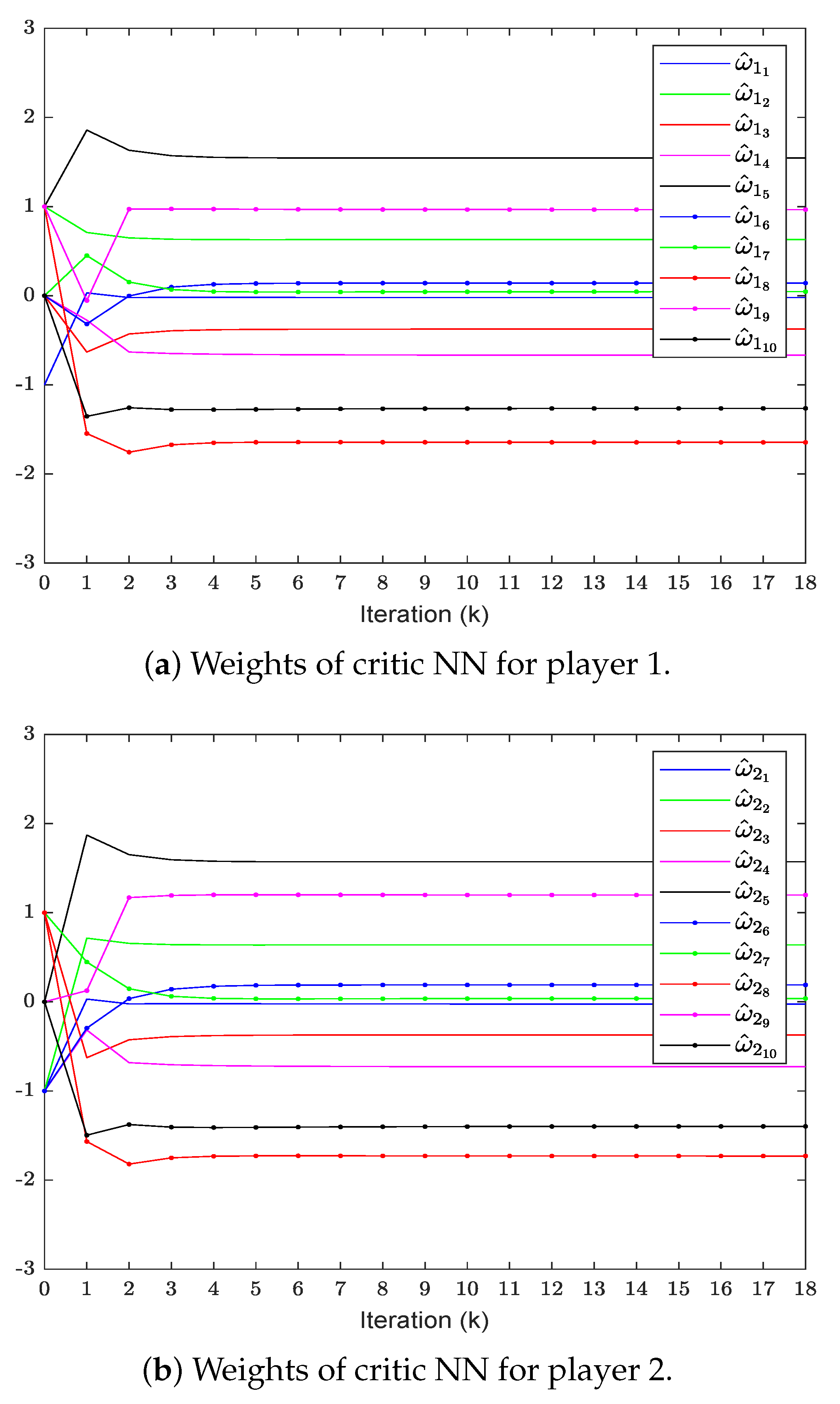
In order to verify the effectiveness of the proposed method, we will compare it with the method in [38] under the same conditions. To save space, this article presents a comparison of only some of the important results. Figure 1 shows the convergence curve of evaluating the weights of the critic NN, which finally converges to

$${\widehat{\omega }}_1={[-0.0213,0.6304,-0.3745,-0.6673,1.5467,0.1415,0.0455,-1.6452,0.9663,1.2640]}^T$$

$${\widehat{\omega }}_2={[-0.0247,0.6392,-0.3716,-0.7285,1.5715,0.1891,0.0372,-1.7302,1.1982,-1.3978]}^T.$$

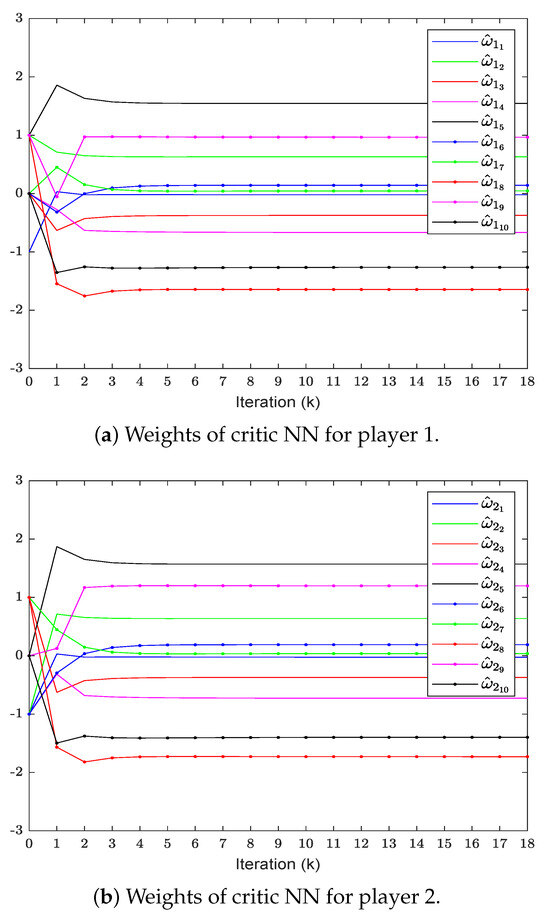
Figure 1. Critic NN weight convergence curve.

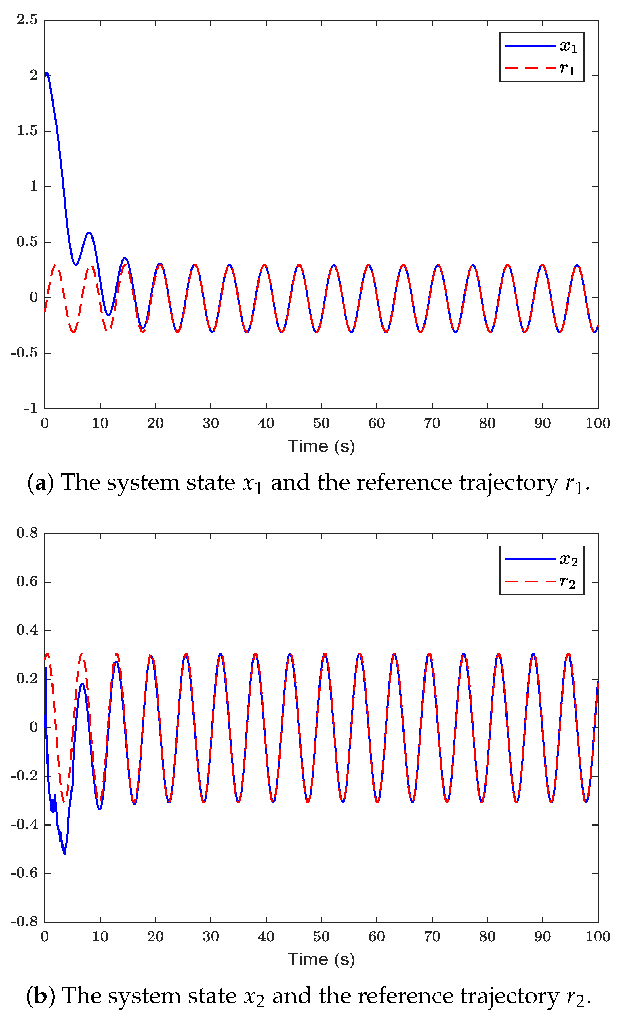
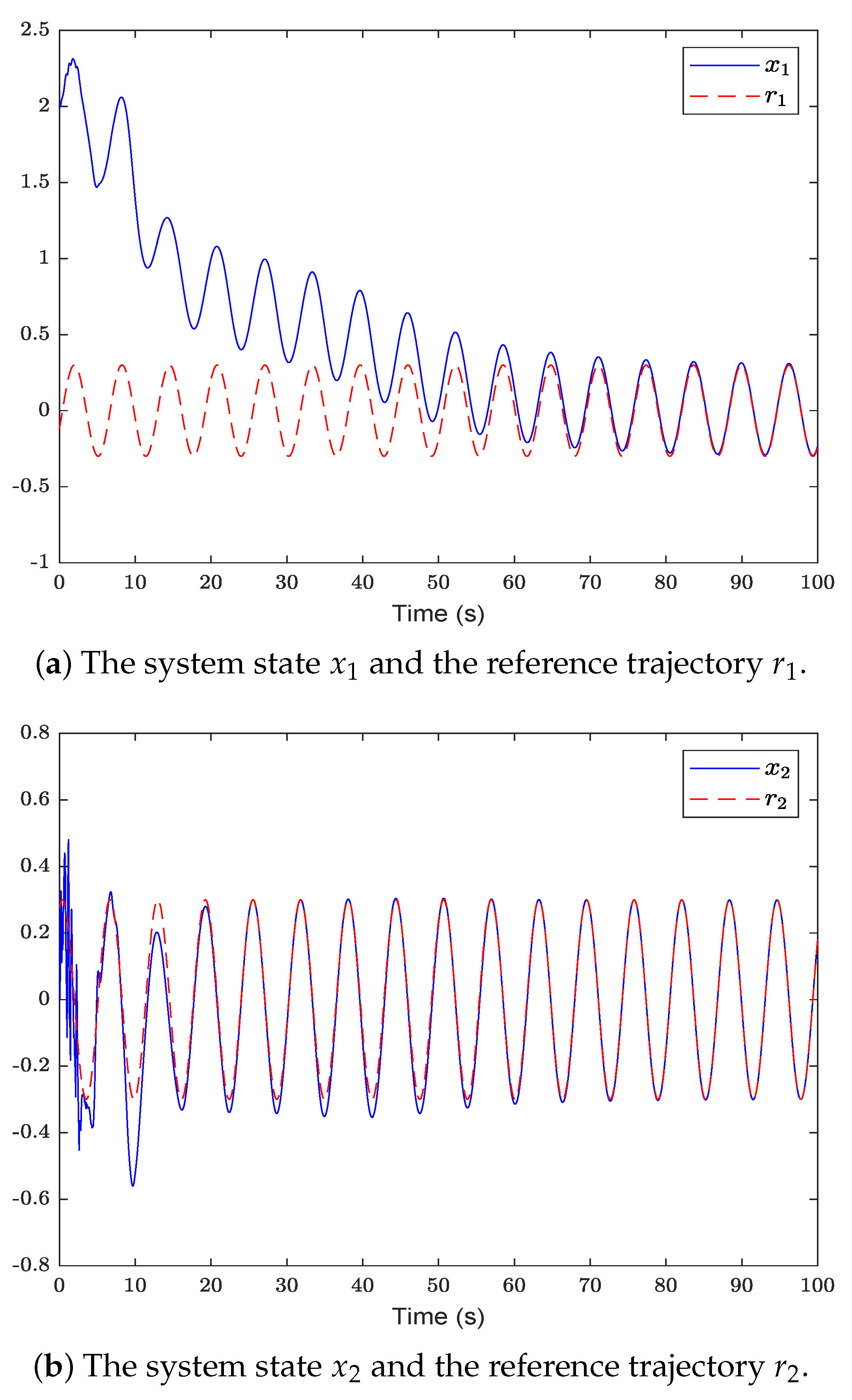
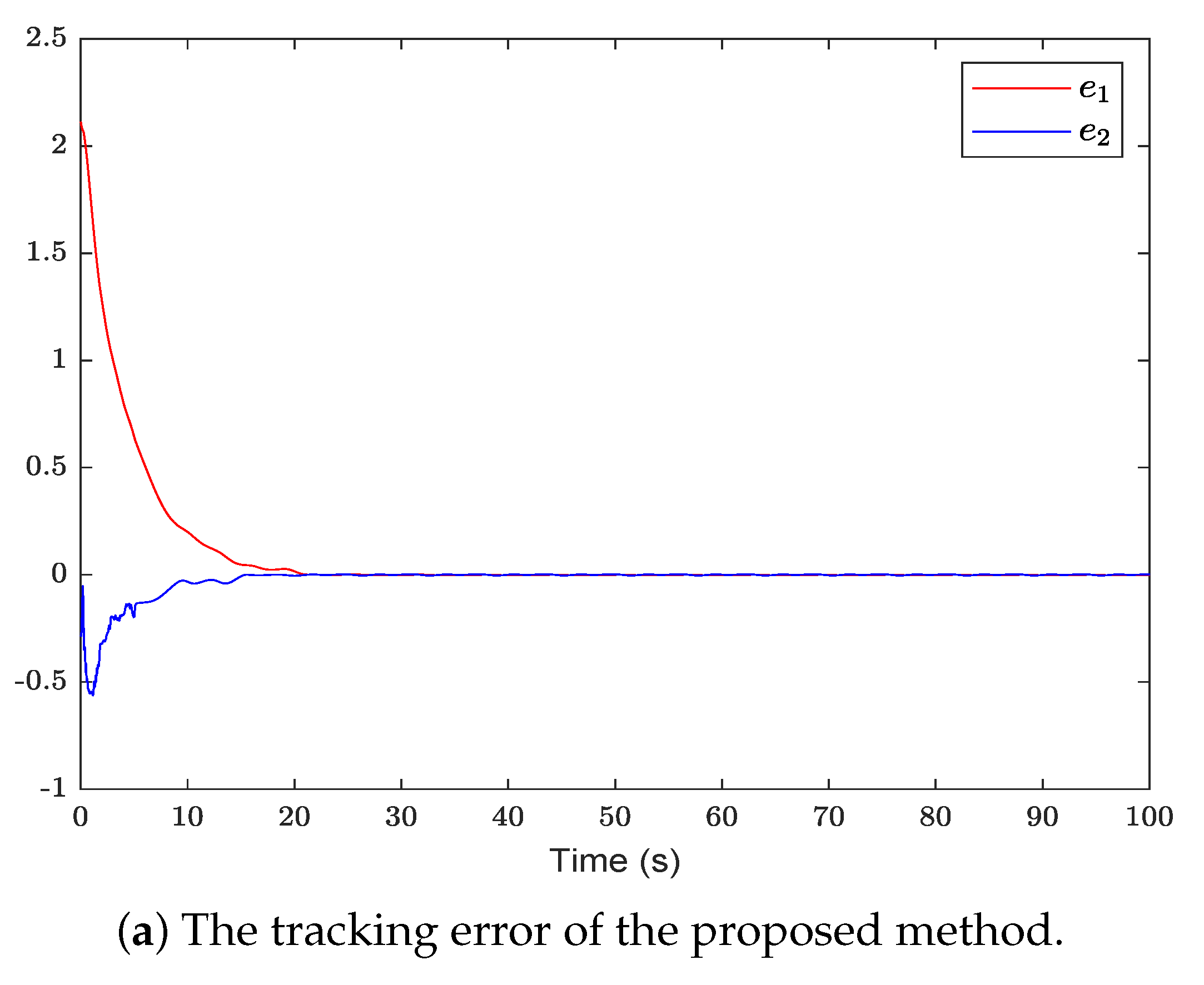
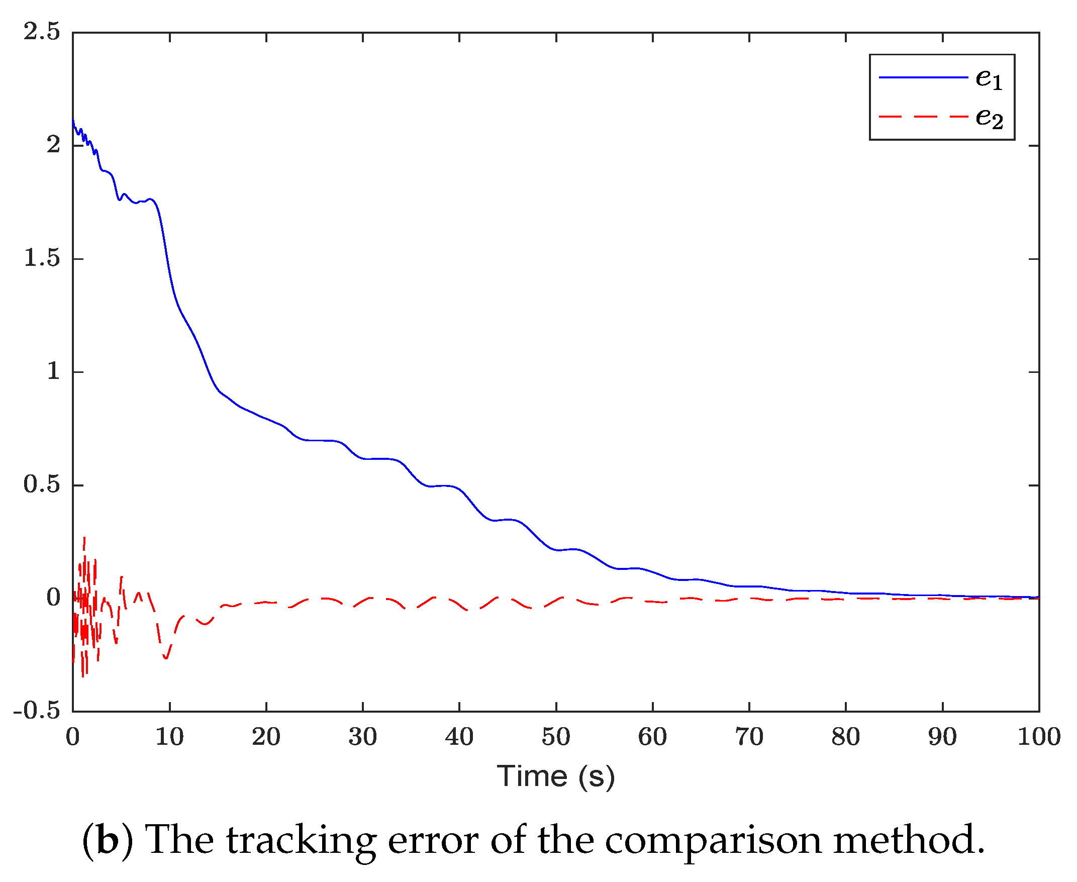
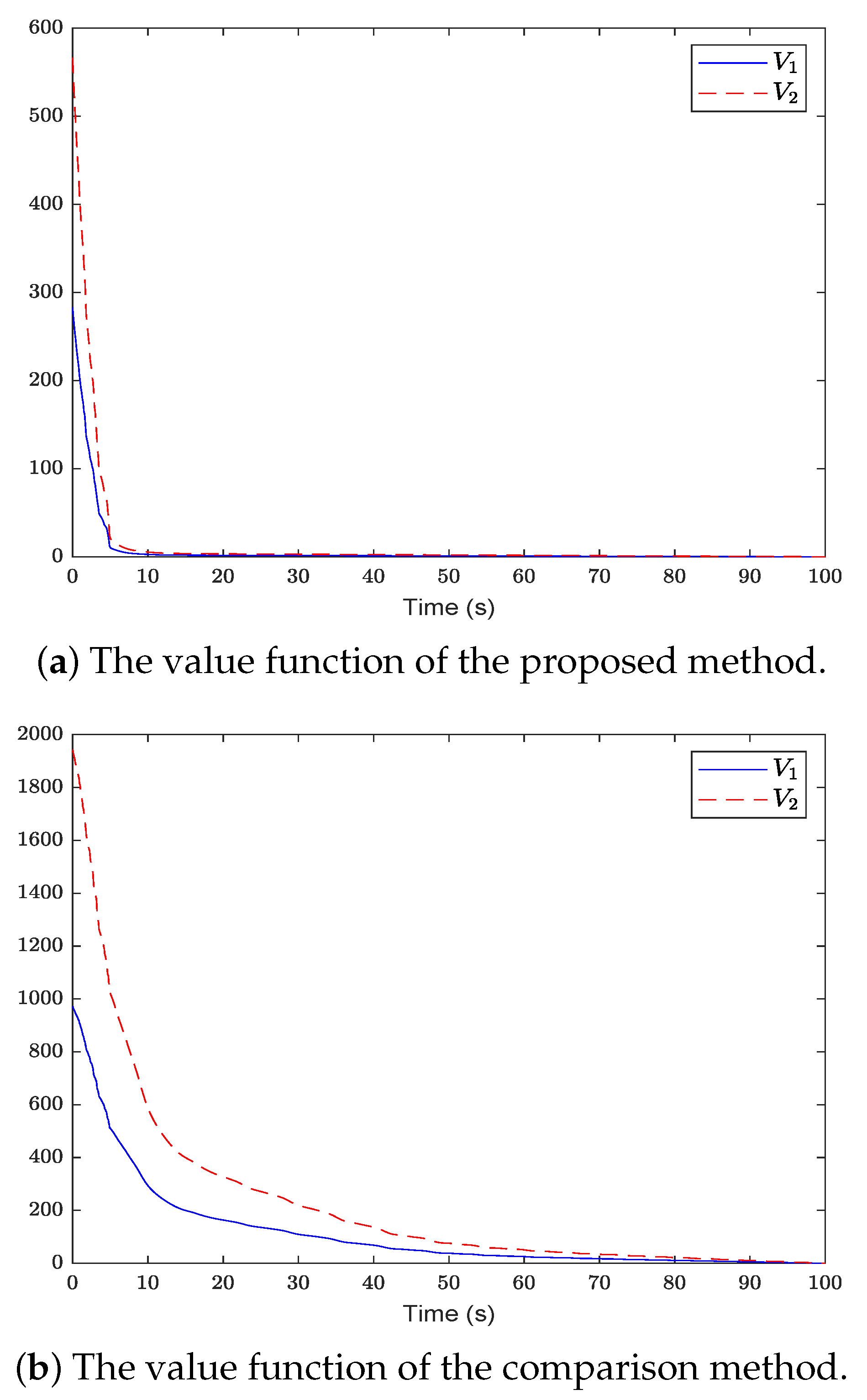
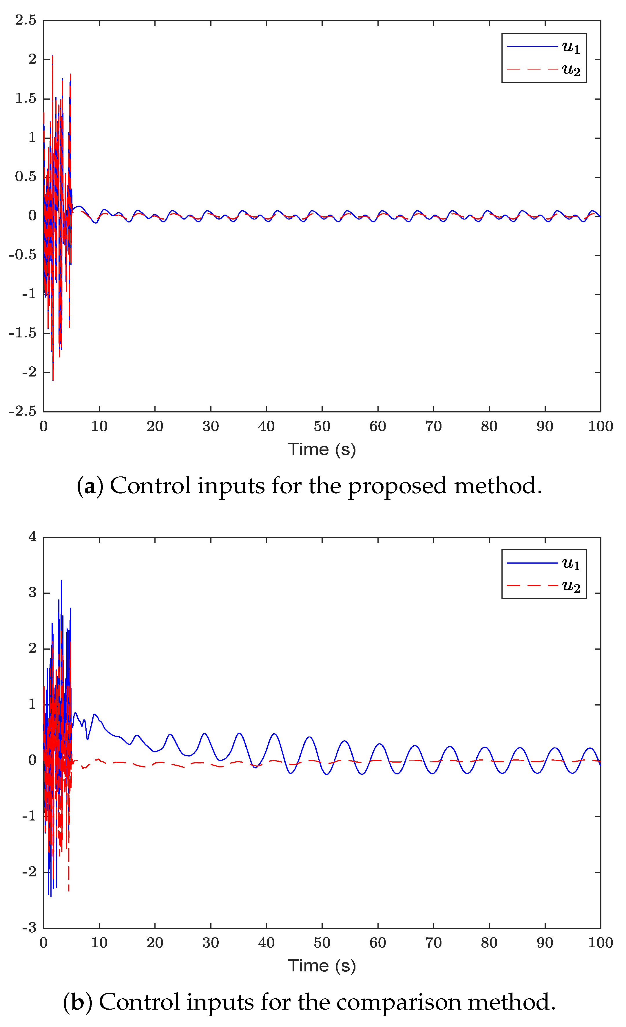
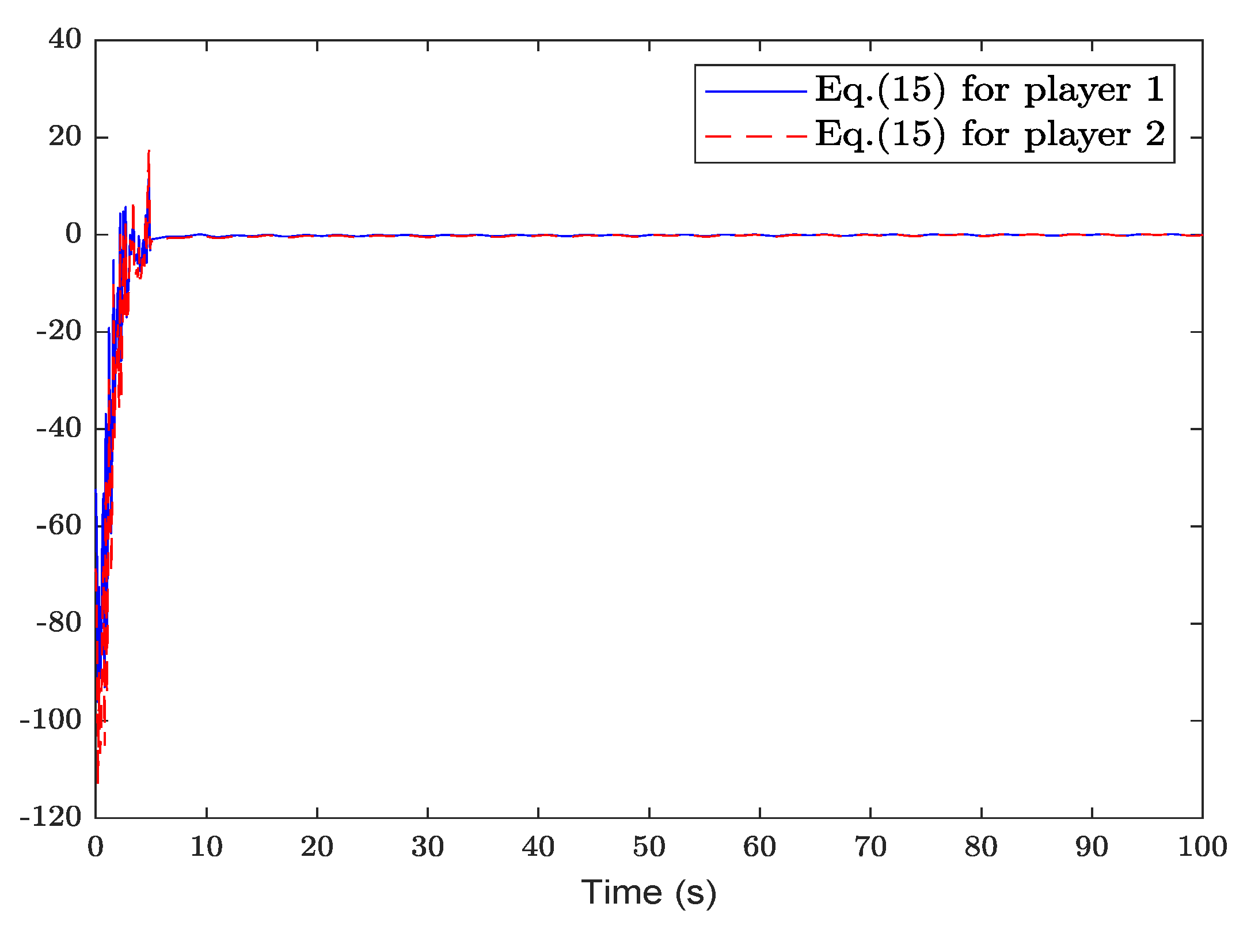
Figure 2 shows the system state $x\left(t\right)$ and reference trajectory $r\left(t\right)$ of the proposed method in this paper. It can be seen that the system state $x\left(t\right)$ can track the reference trajectory $r\left(t\right)$ after 20 s. Figure 3 shows the system state $x\left(t\right)$ and reference trajectory $r\left(t\right)$ of the method given in [38]. It can be seen that the reference trajectory $r\left(t\right)$ can be tracked in the system state $x\left(t\right)$ only after 90 s. In Figure 4a,b are the evolution curves of the tracking error of the proposed method in this paper and that of the proposed method in [38], respectively. From Figure 4, it is easy to see that the tracking error convergence speed of the proposed method in this paper is faster than that used in [38]. Figure 5 shows a comparison between the value function obtained by the proposed method and that obtained by the method used in [38]. It is easy to see that the value function of the proposed method in this paper is smaller both at the initial moment and the final moment, that is, the optimal control obtained in this paper is better than that obtained by the comparison method. The control inputs of the proposed method are compared with that of the comparison method in Figure 6. Figure 7 is an evolution curve approximating the HJ equation. For Equation (15), optimal control can make the left end of Equation (15) equal to zero, but for a non-optimal control it is not necessarily possible to make the left end of Equation (15) equal to zero. In this paper, approximate optimal control is used to approximate optimal control, so it is necessary to bring the obtained approximate optimal control back to the right end of Equation (15) to verify whether it is equal to zero. By observing Figure 7, it can be seen that the optimal approximate control obtained by this method makes the left end of Equation (15) equal to zero, i.e., the optimal approximate control ${\widehat{u}}_i^k$ converges to the optimal control $u_i^{*}$.

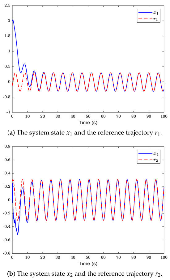
Figure 2. The system state $x\left(t\right)$ of the proposed method is compared with the reference trajectory $r\left(t\right)$.

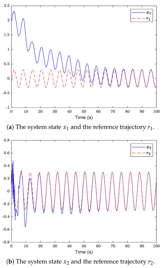
Figure 3. The system state $x\left(t\right)$ of the comparison method is compared with the reference trajectory $r\left(t\right)$.

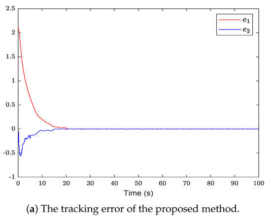
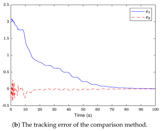
Figure 4. The evolution curve of the tracking error of the proposed method is compared with that of the comparison method.

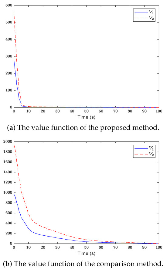
Figure 5. The comparison between the value function of the proposed method and that of the comparison method.

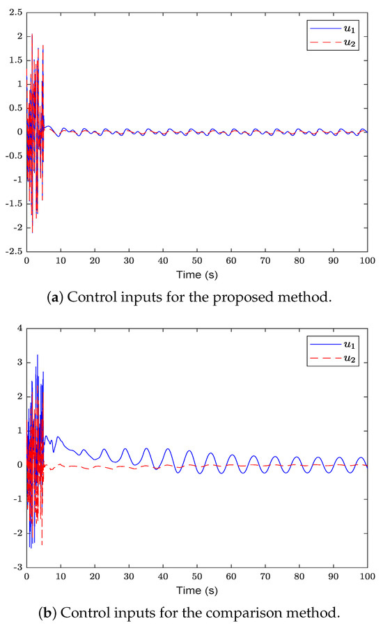
Figure 6. The control inputs of the proposed method are compared with that of the comparison method.

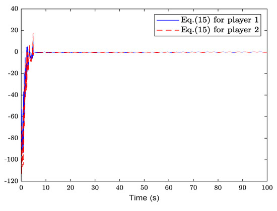
Figure 7. The evolution of (15).

6. Conclusions

To tackle the OTCP for nonlinear CT NZS differential game systems with unknown drift dynamics, an IRL method based on PI is proposed. Because the HJB equation is an NPDE that cannot be solved directly, the single-layer critic NN is used for approximating the value function of each player, and the LS method is used to update the weight of the NN. Due to the stability of the tracking error dynamics system, the approximate solutions converge to a Nash equilibrium, and the convergence of the weights of the NN is strictly proven. Finally, the validity of Algorithm 2 is verified by MATLAB simulation, and the comparison yields faster convergence and shows the higher convergence accuracy of this method.

References

- Jiang, Y.; Jiang, Z. Robust Adaptive Dynamic Programming for Large-Scale Systems with an Application to Multimachine Power Systems. IEEE Trans. Circuits Syst. Express Briefs 2012, 59, 693–697. [Google Scholar] [CrossRef]
- Bian, T.; Jiang, Y.; Jiang, Z.P. Decentralized Adaptive Optimal Control of Large-Scale Systems with Application to Power Systems. IEEE Trans. Ind. Electron. 2015, 62, 2439–2447. [Google Scholar] [CrossRef]
- Kirk, D.E. Optimal Control Theory: An Introduction; Dover Publications: New York, NY, USA, 2004. [Google Scholar]
- Rodrigues, L. Affine Quadratic Optimal Control and Aerospace Applications. IEEE Trans. Aerosp. Electron. Syst. 2021, 57, 795–805. [Google Scholar] [CrossRef]
- Lu, K.; Yu, H.; Liu, Z.; Han, S.; Yang, J. Inverse Optimal Adaptive Control of Canonical Nonlinear Systems with Dynamic Uncertainties and Its Application to Industrial Robots. IEEE Trans. Ind. Inf. 2024, 20, 5318–5327. [Google Scholar] [CrossRef]
- Alfred, D.; Czarkowski, D.; Teng, J. Reinforcement Learning-Based Control of a Power Electronic Converter. Mathematics 2024, 12, 671. [Google Scholar] [CrossRef]
- Mu, C.; Zhen, N.; Sun, C.; He, H. Data-Driven Tracking Control with Adaptive Dynamic Programming for a Class of Continuous-Time Nonlinear Systems. IEEE Trans. Cybern. 2017, 47, 1460–1470. [Google Scholar] [CrossRef]
- Abu-Khalaf, M.; Lewis, F.L. Nearly optimal control laws for nonlinear systems with saturating actuators using a neural network HJB approach. Automatica 2005, 41, 779–791. [Google Scholar] [CrossRef]
- Lv, Y.; Na, J.; Yang, Q.; Wu, X.; Guo, Y. Online adaptive optimal control for continuous-time nonlinear systems with completely unknown dynamics. Int. J. Control 2015, 89, 99–112. [Google Scholar] [CrossRef]
- Xiao, G.; Zhang, H. Convergence Analysis of Value Iteration Adaptive Dynamic Programming for Continuous-Time Nonlinear Systems. IEEE Trans. Cybern. 2024, 54, 1639–1649. [Google Scholar] [CrossRef] [PubMed]
- Wang, G. Distributed control of higher-order nonlinear multi-agent systems with unknown non-identical control directions under general directed graphs. Automatica 2019, 110, 108559. [Google Scholar] [CrossRef]
- Chen, B.; Hu, J.; Zhao, Y.; Ghosh, B.K. Finite-time observer based tracking control of uncertain heterogeneous underwater vehicles using adaptive sliding mode approach. Neurocomputing 2022, 481, 322–332. [Google Scholar] [CrossRef]
- Wang, G. Consensus Algorithm for Multiagent Systems with Nonuniform Communication Delays and Its Application to Nonholonomic Robot Rendezvous. IEEE Trans. Control Netw. Syst. 2023, 10, 1496–1507. [Google Scholar] [CrossRef]
- Bidram, A.; Davoudi, A.; Lewis, F.L.; Guerrero, J.M. Distributed Cooperative Secondary Control of Microgrids Using Feedback Linearization. IEEE Trans. Power Syst. 2013, 28, 3462–3470. [Google Scholar] [CrossRef]
- Kodagoda, K.R.S.; Wijesoma, W.S.; Teoh, E.K. Fuzzy speed and steering control of an AGV. IEEE Trans. Control Syst. Technol. 2002, 10, 112–120. [Google Scholar] [CrossRef]
- Song, R.; Wei, Q.; Zhang, H.; Lewis, F.L. Discrete-Time Non-Zero-Sum Games with Completely Unknown Dynamics. IEEE Trans. Cybern. 2021, 51, 2929–2943. [Google Scholar] [CrossRef] [PubMed]
- Karg, P.; Kopf, F.; Braun, C.A.; Hohmann, S. Excitation for Adaptive Optimal Control of Nonlinear Systems in Differential Games. IEEE Trans. Autom. Control 2023, 68, 596–603. [Google Scholar] [CrossRef]
- Li, H.; Wei, Q. Initial Excitation-Based Optimal Control for Continuous-Time Linear Nonzero-Sum Games. IEEE Trans. Syst. Man Cybern. Syst. 2024, 1–12. [Google Scholar] [CrossRef]
- Nash, J.F. Non-cooperative Games. In Classics in Game Theory; Princeton University Press: Princeton, NJ, USA, 1951. [Google Scholar]
- Clemhout, S.; Wan, H.Y. Differential games-Economic applications. Handb. Game Theory Econ. Appl. 1994, 2, 801–825. [Google Scholar]
- Zhang, Z.; Xu, J.; Fu, M. Q-Learning for Feedback Nash Strategy of Finite-Horizon Nonzero-Sum Difference Games. IEEE Trans. Cybern. 2022, 52, 9170–9178. [Google Scholar] [CrossRef]
- Savku, E. A Stochastic Control Approach for Constrained Stochastic Differential Games with Jumps and Regimes. Mathematics 2023, 11, 3043. [Google Scholar] [CrossRef]
- Case, J.H. Toward a Theory of Many Player Differential Games. SIAM J. Control 1969, 7, 179–197. [Google Scholar] [CrossRef]
- Werbos, P.J. Approximate dynamic programming for real-time control and neural modeling. In Handbook of Intelligent Control Neural Fuzzy & Adaptive Approaches; Van Nostrand Reinhold: New York, NY, USA, 1992; pp. 493–525. [Google Scholar]
- Song, R.; Yang, G. Online solving Nash equilibrium solution of N-player nonzero-sum differential games via recursive least squares. Soft Comput. 2023, 27, 16659–16673. [Google Scholar] [CrossRef]
- Zhang, H.; Cui, L.; Luo, Y. Near-Optimal Control for Nonzero-Sum Differential Games of Continuous-Time Nonlinear Systems Using Single-Network ADP. IEEE Trans. Cybern. 2013, 43, 206–216. [Google Scholar] [CrossRef] [PubMed]
- Vrabie, D.; Lewis, F. Neural network approach to continuous-time direct adaptive optimal control for partially unknown nonlinear systems. Neural Netw. 2009, 22, 237–246. [Google Scholar] [CrossRef] [PubMed]
- Liu, D.; Li, H.; Wang, D. Online Synchronous Approximate Optimal Learning Algorithm for Multi-Player Non-Zero-Sum Games with Unknown Dynamics. IEEE Trans. Syst. Man Cybern. Syst. 2014, 44, 1015–1027. [Google Scholar] [CrossRef]
- Zhang, H.; Jiang, H.; Luo, C.; Xiao, G. Discrete-Time Nonzero-Sum Games for Multiplayer Using Policy-Iteration-Based Adaptive Dynamic Programming Algorithms. IEEE Trans. Cybern. 2017, 47, 3331–3340. [Google Scholar] [CrossRef]
- Wei, Q.; Zhu, L.; Song, R.; Zhang, P.; Liu, D.; Xiao, J. Model-Free Adaptive Optimal Control for Unknown Nonlinear Multiplayer Nonzero-Sum Game. IEEE Trans. Neural Netw. Learn. Syst. 2022, 33, 879–892. [Google Scholar] [CrossRef] [PubMed]
- Jiang, H.; Zhang, H.; Zhang, K.; Cui, X. Data-driven adaptive dynamic programming schemes for non-zero-sum games of unknown discrete-time nonlinear systems. Neurocomputing 2018, 275, 649–658. [Google Scholar] [CrossRef]
- Zhang, Q.; Zhao, D. Data-Based Reinforcement Learning for Nonzero-Sum Games with Unknown Drift Dynamics. IEEE Trans. Cybern. 2019, 49, 2874–2885. [Google Scholar] [CrossRef]
- Qin, C.; Shang, Z.; Zhang, Z.; Zhang, D.; Zhang, J. Robust Tracking Control for Non-Zero-Sum Games of Continuous-Time Uncertain Nonlinear Systems. Mathematics 2022, 10, 1904. [Google Scholar] [CrossRef]
- Kiumarsi, B.; Lewis, F.L. Actor-Critic-Based Optimal Tracking for Partially Unknown Nonlinear Discrete-Time Systems. IEEE Trans. Neural Netw. Learn. Syst. 2015, 26, 140–151. [Google Scholar] [CrossRef]
- Lv, Y.; Ren, X.; Na, J. Adaptive Optimal Tracking Controls of Unknown Multi-input Systems based on Nonzero-Sum Game Theory. J. Frankl. Inst. 2019, 356, 8255–8277. [Google Scholar] [CrossRef]
- Wen, Y.; Zhang, H.; Su, H.; Ren, H. Optimal tracking control for non-zero-sum games of linear discrete-time systems via off-policy reinforcement learning. Optim. Control Appl. Methods 2020, 41, 1233–1250. [Google Scholar] [CrossRef]
- Qin, C.; Qiao, X.; Wang, J.; Zhang, D.; Hou, Y.; Hu, S. Barrier-Critic Adaptive Robust Control of Nonzero-Sum Differential Games for Uncertain Nonlinear Systems with State Constraints. IEEE Trans. Syst. Man Cybern. Syst. 2024, 54, 50–63. [Google Scholar] [CrossRef]
- Zhao, J. Neural networks-based optimal tracking control for nonzero-sum games of multi-player continuous-time nonlinear systems via reinforcement learning. Neurocomputing 2020, 412, 167–176. [Google Scholar] [CrossRef]
- Modares, H.; Lewis, F.L. Optimal tracking control of nonlinear partially-unknown constrained-input systems using integral reinforcement learning. Automatica 2014, 50, 1780–1792. [Google Scholar] [CrossRef]
- BaÅŸar, T.; Olsder, G.J. Dynamic Noncooperative Game Theory, 2nd ed.; SIAM: Philadelphia, PA, USA, 1999. [Google Scholar]
- Amvoudakis, K.G.V.; Lewis, F.L. Multi-player non-zero-sum games: Online adaptive learning solution of coupled Hamilton-Jacobi equations. Automatica 2011, 47, 1556–1569. [Google Scholar] [CrossRef]
- Kamalapurkar, R.; Klotz, J.R.; Dixon, W.E. Concurrent learning-based approximate feedback-Nash equilibrium solution of N-player nonzero-sum differential games. IEEE/CAA J. Autom. Sin. 2014, 1, 239–247. [Google Scholar] [CrossRef]
- Luo, B.; Wu, H.N.; Huang, T. Off-policy reinforcement learning for H∞ control design. IEEE Trans. Cybern. 2015, 45, 65–76. [Google Scholar] [CrossRef]
- Jiang, Y.; Jiang, Z.P. Robust Adaptive Dynamic Programming and Feedback Stabilization of Nonlinear Systems. IEEE Trans. Neural Netw. Learn. Syst. 2014, 25, 882–893. [Google Scholar] [CrossRef]
Disclaimer/Publisher’s Note: The statements, opinions and data contained in all publications are solely those of the individual author(s) and contributor(s) and not of MDPI and/or the editor(s). MDPI and/or the editor(s) disclaim responsibility for any injury to people or property resulting from any ideas, methods, instructions or products referred to in the content. |
© 2024 by the authors. Licensee MDPI, Basel, Switzerland. This article is an open access article distributed under the terms and conditions of the Creative Commons Attribution (CC BY) license (https://creativecommons.org/licenses/by/4.0/).