Adaptive Fixed-Time Safety Concurrent Control of Vehicular Platoons with Time-Varying Actuator Faults under Distance Constraints

Abstract

This paper investigates the fault-tolerant control problem for vehicular platoons with time-varying actuator fault directions and distance constraints. A bias constraint function is introduced to convert the asymmetric constraints into symmetric ones, based on which a unified barrier Lyapunov function (BLF) method is proposed to ensure distance constraints. Further, an adaptive fixed-time fault-tolerant controller in the context of a sliding mode control technique is proposed, wherein a new Nussbaum function is adopted to address the effects of unknown time-varying actuator fault directions. It is proved that both individual vehicle stability and string stability can all be guaranteed, and the effectiveness of the proposed algorithm is verified through numerical simulations.

1. Introduction

Due to the good interaction between vehicles, vehicular platoon control, as an important part of an intelligent transportation system (ITS), has shown great potential to deal with various traffic issues, such as traffic congestion, air pollution, highway safety and so on [1,2,3]. Driving at a small distance can reduce the air resistance on the vehicle, which in turn reduces fuel consumption and increases road capacity [4]. Yet, it is known that small gaps between connected vehicles are the most likely to cause collisions. To this end, distance constraints, from the safety perspective, are issues that are worth investigating [5,6]. At present, there are two main effective methods proposed to deal with spacing constraints, namely, the prescribed performance control method [7,8] and the barrier Lyapunov function (BLF) method [9], among which the BLF method can satisfy stability and safety requirements at the same time, as described in [10,11], which promotes its application in vehicular platoon control. The work in [9] focuses on dealing with symmetric and asymmetric distance restrictions by utilizing symmetric and asymmetric BLF, respectively, and more similar results can be found in [12,13,14]. It is worth noting that the results above depend on the type (i.e., symmetric and asymmetric) of distance constraints, which are time-varying and not available previously, in some cases.

Actuator fault, as a common type of actuator nonlinearity, is an inevitable factor that may degrade system performance, and even lead to system instability for a practical physical system [15,16]. In recent years, researchers have made great contributions to the fault-tolerant control of vehicles [8,9,14,17,18,19]. However, most existing results are all based on the classical actuator fault model, and more attention has been paid to the loss of effectiveness and bias fault, yet the direction of the fault is ignored. As we all know, the direction of the fault varies with time and may be unknown in the actual operation. Therefore, it is of great theoretical and practical significance to achieve the fault tolerance of actuator fault with unknown directions. To handle an actuator fault with unknown directions, the Nussbaum function technique is adopted in [9,14], which is also used to in this paper but for a third-order nonlinear vehicular platoon system, and string stability is also considered.

Inspired by the aforementioned analysis, a novel adaptive fixed-time fault-tolerant control scheme is designed for a third-order vehicular platoon system with unknown actuator fault directions and distance constraints. The main contributions are summarized as follows:

(1)

A new Nussbaum function with smaller amplitudes is designed, with which the unknown time-varying actuator fault directions are dealt with, without depending on the precise boundary values for the efficiency loss factor.

(2)

A unified BLF method based on the bias constraint function is proposed, which can transform the asymmetric constraint into a symmetric one, making the control design simpler.

(3)

Together with the proposed Nussbaum function and BLF method, an adaptive fixed-time sliding mode control scheme is developed for a third-order platoon system, with which the individual vehicle stability and string stability can all be guaranteed within a settling time.

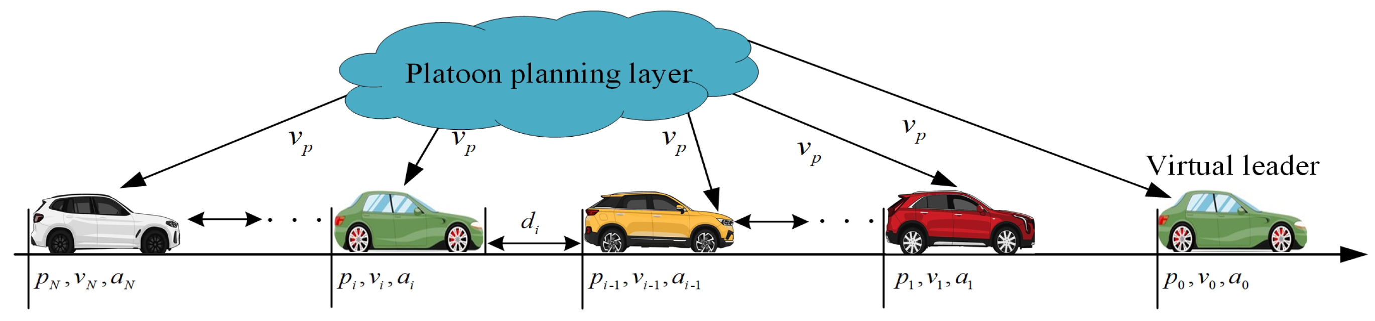
2. Preliminaries and Problem Formulation

2.1. Preliminaries

Lemma 1

([20]). For the continuous radially unbounded function $V\left(z\left(t\right)\right):{\mathbb{R}}^n\to {\mathbb{R}}^{+}$ such that

$$\begin{array}{c}\hfill \dot{V}\left(z\left(t\right)\right)\le -\alpha V^1\left(z\left(t\right)\right)-\beta V^2\left(z\left(t\right)\right)+\varpi ,t\ge 0,\end{array}$$

(1)

where $\alpha >0$, $\beta >0$, $0<{ }_1<1$, ${ }_2>1$, if $\varpi =0$, then $\dot{z}\left(t\right)=f\left(z\right)$ is globally fixed-time stable (GFxTS), and the settling time T is bounded as

$$\begin{array}{c}\hfill T\le T_{max}={\displaystyle \frac{1}{\alpha \left(1-{ }_1\right)}}+{\displaystyle \frac{1}{\beta \left({ }_2-1\right)}},\end{array}$$

(2)

otherwise, if $0<\varpi <\infty$, then the system is $\dot{z}\left(t\right)=f\left(z\right)$ practically fixed-time stable (PFxTS). Moreover, the residual set of the system is

$$\underset{t\to T}{lim}|V\left(z\left(t\right)\right)\le min\left\{{\alpha }^{{\displaystyle \frac{-1}{{ }_1}}}{\left({\displaystyle \frac{\varpi }{1-\tilde{\theta }}}\right)}^{{\displaystyle \frac{1}{{ }_1}}},{\beta }^{{\displaystyle \frac{-1}{{ }_2}}}{\left({\displaystyle \frac{\varpi }{1-\tilde{\theta }}}\right)}^{{\displaystyle \frac{1}{{ }_2}}}\right\},$$

(3)

where $\tilde{\theta }$ is scalar and satisfies $\tilde{\theta }$, and the settling time T is bounded as

$$\begin{array}{c}\hfill T\le T_{max}={\displaystyle \frac{1}{\alpha \tilde{\theta }\left(1-{ }_1\right)}}+{\displaystyle \frac{1}{\beta \tilde{\theta }\left({ }_2-1\right)}}.\end{array}$$

(4)

Lemma 2

([21]). The following inequalities hold

$$\begin{array}{cc}\hfill s^{1+k}-c^{1+k}& \le {(c-s)}^{1+k},\hfill \\ \hfill z^k(\tau -z)& \le {\displaystyle \frac{1}{1+k}}\left({\tau }^{k+1}-z^{k+1}\right),\hfill \end{array}$$

(5)

when $c>0$, $s\le c$, $z\ge 0$, $\tau >0$, and $k>0$.

Lemma 3

([22]). For positive parameters ${\epsilon }_1,{\epsilon }_2,\cdots ,{\epsilon }_G$, one has

$$\begin{array}{cc}\hfill & \sum _{i=1}^G{{\epsilon }_i^n\ge \left(\sum _{i=1}^G{\epsilon }_i\right)}^n,0<n\le 1,\hfill \\ \hfill & \sum _{i=1}^G{{\epsilon }_i^n\ge M^{1-n}\left(\sum _{i=1}^G{\epsilon }_i\right)}^n,1<n\le \infty .\hfill \end{array}$$

(6)

Lemma 4

([23]). For any positive constant ϵ, we have

$$ln{\displaystyle \frac{{ϵ}^2}{{ϵ}^2-s^2\left(t\right)}}\le {\displaystyle \frac{s^2\left(t\right)}{{ϵ}^2-s^2\left(t\right)}},\mathit{if}\left|s\left(t\right)\right|<ϵ.$$

(7)

Lemma 5

([24]). There exist two smooth functions, $V\left(t\right)$ and ${\delta }_i\left(t\right)$, that are defined on $[0,t_f)$, satisfying $V\left(t\right)>0$, $t\in [0,t_f)$, and $N\left({\delta }_i\left(t\right)\right)$ is a smooth Nussbaum function. $V\left(t\right)$, ${\delta }_i\left(t\right)$, and ${\sum }_{i=1}^N{\int }_0^t[{\rho }_i\left(\tau \right)N\left({\delta }_i\left(\tau \right)\right)+1]{\dot{\delta }}_i\left(\tau \right)d\tau$ must be bounded on $[0,t_f)$, when the following inequality holds:

$$V\left(t\right)\le c_0+\sum _{i=1}^N{\int }_0^t[{\rho }_i\left(\tau \right)N\left({\delta }_i\left(\tau \right)\right)+1]{\dot{\delta }}_i\left(\tau \right)d\tau ,\forall t\in [0,t_f),$$

(8)

while $c_0$ is a constant and ${\rho }_i\left(t\right)$ is a time-varying variable which takes a nonzero value from a closed interval.

2.2. Vehicle Dynamics

In this paper, a concurrent vehicular platoon system, containing N vehicles driving on a straight road (see Figure 1), is considered, and the dynamics for vehicle i ($i\in 1,2,\cdots ,N$) are adopted [18]:

$$\begin{array}{cc}\hfill {\dot{p}}_i\left(t\right)& =v_i\left(t\right),\hfill \\ \hfill {\dot{v}}_i\left(t\right)& =a_i\left(t\right),\hfill \\ \hfill {\dot{a}}_i\left(t\right)& =u_{ai}\left(t\right)+f_i(v_i,a_i)+{\omega }_i\left(t\right),\hfill \end{array}$$

(9)

with

$$\begin{array}{c}\hfill f_i\left(v_i,a_i\right)=-{\displaystyle \frac{1}{m_i{\tau }_i}}\left[{\rho }_{ai}{O}_i{C}_{ai}\left({\displaystyle \frac{1}{2}}{v}_i^2+{\tau }_i{v}_i{a}_i\right)+{\Xi }_i\right]-{\displaystyle \frac{1}{{\tau }_i}}{a}_i,\end{array}$$

(10)

and

$$\begin{array}{c}\hfill u_i\left(t\right)={\displaystyle \frac{1}{m_i{\tau }_i}}{\varsigma }_i\left(t\right),\end{array}$$

(11)

where $p_i\left(t\right)$, $v_i\left(t\right)$, and $a_i\left(t\right)$ denote position, velocity, and acceleration, respectively. ${\Xi }_i$ denotes the road slope function, and the definitions of the remaining parameters are given in

Table 1. The Definitions of the Model Parameters.

$m_i$	The vehicle’s mass	${\omega }_i\left(t\right)$	The external disturbances
${\rho }_{ai}$	The air density	$C_{ai}$	The drag coefficient
$O_i$	The frontal cross-area	$u_i\left(t\right)$	The control input
${\tau }_i$	The engine time constant	${\varsigma }_i\left(t\right)$	The engine/brake input

.

As a practical physical system, the actuator faults are inevitable. Thus, the actuator fault with time-varying direction is considered [18]:

$$\begin{array}{c}\hfill u_{ai}={\rho }_i(t,t_{\rho ,i})u_i\left(t\right)+r_i(t,t_{r,i}),\end{array}$$

(12)

where ${\rho }_i(t,t_{\rho ,i})$ and $r_i(t,t_{r,i})$ denote the fault efficiency factor and bias fault, respectively, $t_{\rho ,i}$ and $t_{r,i}$ are unknown fault time instants. The fault direction is determined by ${\rho }_i(t,t_{\rho ,i})$, i.e., if ${\rho }_i(t,t_{\rho ,i})>0$, the fault direction is forward, otherwise, the fault direction is in reverse.

Further, substituting (12) into (9) yields:

$$\begin{array}{cc}\hfill {\dot{p}}_i\left(t\right)& =v_i\left(t\right),\hfill \\ \hfill {\dot{v}}_i\left(t\right)& =a_i\left(t\right),\hfill \\ \hfill {\dot{a}}_i\left(t\right)& ={\rho }_i(t,t_{\rho ,i})u_i\left(t\right)+f_i(v_i,a_i)+{\omega }_i\left(t\right)+r_i(t,t_{r,i}).\hfill \end{array}$$

(13)

As described in [18], the nonlinear function $f_i(v_i,a_i)$ cannot be exactly determined due to parameter uncertainties, which will be approximated by RBFNN technique as:

$$\begin{array}{c}\hfill f_i(v_i,a_i)=W_i^T{\xi }_i\left(Z_i\right)+{\epsilon }_i,\end{array}$$

(14)

where $W_i^T$ is the ideal parameter vector, ${\xi }_i\left(Z_i\right)$ is the Gaussian basis function vector, and ${\epsilon }_i$ denotes the approximation error satisfying ${\epsilon }_i\le {\overline{\epsilon }}_i$ with ${\overline{\epsilon }}_i$ being an unknown positive constant.

Assumption 1.

The parameters ${\rho }_i(t,t_{\rho ,i})$, $r_i(t,t_{r,i})$, and ${\omega }_i\left(t\right)$ are bounded, i.e., $0<{\underline{\rho }}_i\le \left|{\rho }_i(t,t_{\rho ,i})\right|\le {\overline{\rho }}_i<\infty$, $\left|r_i(t,t_{r,i})\right|\le {\overline{r}}_i$, ${\omega }_i\left(t\right)\le {\overline{\omega }}_i$ with ${\underline{\rho }}_i$, ${\overline{\rho }}_i$, ${\overline{r}}_i$ and ${\overline{\omega }}_i$ as unknown nonnegative constants.

2.3. Distance Constraints

From Figure 1, it is obvious that vehicle 1 has no preceding car, which makes it difficult to design a controller for it directly. To this end, the virtual vehicle strategy is introduced, with which the controller for each vehicle can be designed under a unified framework. Here, the state of the virtual vehicle (label 0) is defined as $(p_0,v_0,a_0)$ with $p_0=v_{p}t$, $v_0=v_p$, and $a_0={\dot{v}}_p$, and $v_p$ can be obtained from the planning layer.

Assumption 2

([25]). The trajectories of $v_p\left(t\right)$, ${\dot{v}}_p\left(t\right)$, and ${\ddot{v}}_p\left(t\right)$ are smooth and bounded, where ${\dot{v}}_p\left(t\right)$ and ${\ddot{v}}_p\left(t\right)$ are the first and second time derivatives of $v_p\left(t\right)$, respectively.

Based on the virtual leader, the distance $d_i\left(t\right)$ between two adjacent vehicles is given by:

$$\begin{array}{c}\hfill d_i\left(t\right)=p_{i-1}\left(t\right)-p_i\left(t\right)-L_i,\mathrm{for}i=1,2,\cdots ,N,\end{array}$$

(15)

where $L_i$ is the length of vehicle i.

In practice, collision avoidance and communication connectivity maintenance are crucial performance indexes that, if violated, may lead to platoon system failure. Therefore, the following distance constraints are considered:

$$\begin{array}{c}\hfill 0<{\Delta }_{col,i}<d_i\left(t\right)<{\Delta }_{con,i},\end{array}$$

(16)

where ${\Delta }_{col,i}$ is the minimum distance to prevent collision and ${\Delta }_{con,i}$ is the maximum distance to maintain communication connectivity.

To achieve concurrent control, while avoiding large inter-vehicle distances at high speeds, and improving string stability, a new spacing policy is employed, and then the tracking error is defined as:

$$\begin{array}{c}\hfill s_i\left(t\right)=d_i\left(t\right)-{\Delta }_{i-1,i}-h_i(v_i\left(t\right)-v_p\left(t\right)),\end{array}$$

(17)

where ${\Delta }_{i-1,i}$ is a desired distance between two adjacent vehicles and satisfies ${\Delta }_{col,i}<{\Delta }_{i-1,i}<{\Delta }_{con,i}$, $h_i$ is the headway time. Together with (16) and (17), the distance constraints are converted into the following error constraint:

$$\begin{array}{c}\hfill {\underline{\Delta }}_i<s_i\left(t\right)<{\overline{\Delta }}_i,\end{array}$$

(18)

where ${\underline{\Delta }}_i={\Delta }_{col,i}-{\Delta }_{i-1,i}$ and ${\overline{\Delta }}_i={\Delta }_{con,i}-{\Delta }_{i-1,i}$.

Further, to better handle asymmetric error constraints (i.e., $\left|{\underline{\Delta }}_i\right|\ne \left|{\overline{\Delta }}_i\right|$), the following error transformation is introduced:

$$\begin{array}{c}\hfill z_i=s_i\left(t\right)+{\Delta }_{bc,i},\end{array}$$

(19)

where ${\Delta }_{bc,i}$ is the bias constraint function.

• Then, the error constraints become

$$-b_{c,i}<z_i<b_{c,i},$$

(20)

with $b_{c,i}\in {\mathbb{R}}_{+}$ as the prescribed constraint function, and $b_{c,i}\left(0\right)>\left|z_i\left(0\right)\right|$. Thus, one can deduce that $|s_i\left(t\right)+{\Delta }_{bc,i}|<b_{c,i}$, which is equivalent to ${\underline{\Delta }}_i<s_i\left(t\right)<{\overline{\Delta }}_i$, where ${\underline{\Delta }}_i=-b_{c,i}-{\Delta }_{bc,i}$ and ${\overline{\Delta }}_i=b_{c,i}-{\Delta }_{bc,i}$.

Remark 1.

Compared with the existing methods [9,12,13,14], the proposed bias state transformation-based method in this paper realizes the conversion of asymmetric constraints into symmetric constraints, based on which various types of distance constraints can be guaranteed by the symmetric BLF method. In addition, the given method relaxes the strict constraints on the sign of the constraint state in real time, and avoids the singularity problem that may arise in the derivation of the sign function.

2.4. Control Objectives

In this paper, we aim to develop an adaptive platoon control methodology, such that the following goals are achieved, despite the presence of dynamic uncertainties, unknown disturbances, time-varying actuator faults and distance constraints:

(1)

Fixed-time individual vehicle stability: A desired inter-vehicle distance can be maintained in a given time $T_i$ (i.e., $\underset{t\to T_i}{lim}{s}_i\to 0$ and $s_i\approx 0$ when $t\ge T_i$).

(2)

Fixed-time string stability: After a given time $T_{i2}$, the inter-vehicle spacing tracking error does not increase along the platoon, that is

$$\left|G_i\left(s\right)\right|=\left|{\displaystyle \frac{E_{i+1}\left(s\right)}{E_i\left(s\right)}}\right|\le 1,\mathrm{when}t\ge T_{i2},$$

(21)

where $E_i\left(s\right)$ denotes the Laplace transform of $s_i\left(t\right)$ and $i\in (1,2,\cdots ,N-1)$.

3. Fixed-Time Sliding Mode Surface and Nussbaum Function

3.1. Sliding Mode Surface Design

To ensure that the objective can be realized with a given time, the fixed-time sliding mode surface is designed:

$$\begin{array}{c}\hfill S_i={\dot{z}}_i+{\lambda }_{1i}{\left|z_i\right|}^{{\nu }_{1i}}\mathrm{sign}\left(z_i\right)+{\lambda }_{2i}{\left|z_i\right|}^{{\nu }_{2i}}\mathrm{sign}\left(z_i\right),\end{array}$$

(22)

with

$$\begin{array}{c}\hfill {\dot{S}}_i={\ddot{z}}_i+{\lambda }_{1i}{\nu }_{1i}{\left|z_i\right|}^{{\nu }_{1i}-1}{\dot{z}}_i+{\lambda }_{2i}{\nu }_{2i}{\left|z_i\right|}^{{\nu }_{2i}-1}{\dot{z}}_i,\end{array}$$

(23)

where $0<{\nu }_{1i}<1$, ${\nu }_{2i}>1$, and ${\lambda }_{1i}$ and ${\lambda }_{2i}$ are positive design constants.

Based on (17) and (19), it can be derived that:

$$\begin{array}{c}\hfill {\dot{z}}_i={\dot{s}}_i+{\dot{\Delta }}_{bc,i},\\ \hfill {\ddot{z}}_i={\ddot{s}}_i+{\ddot{\Delta }}_{bc,i},\end{array}$$

(24)

with

$$\begin{array}{c}\hfill {\dot{s}}_i=v_{i-1}-v_i-h_i(a_i-{\dot{v}}_p),\\ \hfill {\ddot{s}}_i=a_{i-1}-a_i-h_i({\dot{a}}_i-{\ddot{v}}_p).\end{array}$$

(25)

To better guarantee the string stability of the platoon, the following coupled sliding mode surface is adopted [26]:

$${\Pi }_i\left(t\right)=\left\{\begin{array}{cc}{\gamma }_i{S}_i\left(t\right)-S_{i+1}\left(t\right),\hfill & i=1,2,\cdots ,N-1,\hfill \\ {\gamma }_i{S}_i\left(t\right),\hfill & i=N,\hfill \end{array}\right.$$

(26)

where ${\gamma }_i$ is a positive parameter coupling the sliding surfaces $S_i\left(t\right)$ and $S_{i+1}\left(t\right)$. Noted that the convergence of the sliding mode surface ${\Pi }_i$ can guarantee the same for $S_i$.

For subsequent controller design, taking the time derivative of ${\Pi }_i\left(t\right)$ yields

$$\begin{array}{c}\hfill {\dot{\Pi }}_i\left(t\right)=\left\{\begin{array}{cc}{\gamma }_i\left\{{\ddot{z}}_i+{\Xi }_i{\dot{z}}_i\right\}-{\dot{S}}_{i+1},\hfill & i=1,2,\cdots ,N-1,\hfill \\ {\gamma }_i\left\{{\ddot{z}}_i+{\Xi }_i{\dot{z}}_i\right\},\hfill & i=N,\hfill \end{array}\right.\end{array}$$

(27)

with ${\Xi }_i={\lambda }_{1i}{\nu }_{1i}{\left|z_i\right|}^{{\nu }_{1i}-1}+{\lambda }_{2i}{\nu }_{2i}{\left|z_i\right|}^{{\nu }_{2i}-1}$.

3.2. Nussbaum Function

To solve the issue of unknown time-varying fault directions, the following Nussbaum function technique is adopted:

$$\begin{array}{c}\hfill N_i\left({\delta }_i\right)={\lambda }_i{\displaystyle \frac{b_i^2{c}_i^2+1}{c_i\sqrt{b_i^2{c}_i^2+1}}}{e}^{b_i{\delta }_i}sin\left({\displaystyle \frac{{\delta }_i}{c_i}}\right),\end{array}$$

(28)

where $i=1,2,\cdots ,N$. ${\lambda }_i$, $b_i$ and $c_i$ are positive constants.

From (28), we can see that $N_i\left({\delta }_i\right)$ is an odd function. Let $D_i\left({\delta }_i\right)={\int }_0^{{\delta }_i}{N}_i\left(x\right)dx$; it is obvious that $D_i\left({\delta }_i\right)$ is an even function. By calculation, we have

$$\begin{array}{c}\hfill D_i\left({\delta }_i\right)={\int }_0^{{\delta }_i}{N}_i\left(x\right)dx={\lambda }_i{e}^{b_i{\delta }_i}sin\left({\displaystyle \frac{{\delta }_i}{c_i}}-{\varphi }_i\right)+{\lambda }_{i}sin{\varphi }_i\end{array}$$

(29)

for ${\delta }_i>0$, where ${\varphi }_i=arccos\left({\displaystyle \frac{b_i{c}_i}{\sqrt{b_i^2{c}_i^2+1}}}\right)$.

Then, the Nussbaum-type function (28) has the following characteristics:

$$\begin{array}{c}\hfill \underset{{\delta }_i\to \infty }{lim}sup{\displaystyle \frac{1}{{\delta }_i}}{\int }_0^{{\delta }_i}{N}_i\left(x\right)dx=+\infty ,\\ \hfill \underset{{\delta }_i\to \infty }{lim}inf{\displaystyle \frac{1}{{\delta }_i}}{\int }_0^{{\delta }_i}{N}_i\left(x\right)dx=-\infty .\end{array}$$

4. Controller Design and Stability Analysis

By combining the proposed sliding mode surface (22) and Nussbaum function (28), an adaptive fixed-time sliding mode controller (FxTSMC) is designed for following vehicles such that platoon objectives can be achieved in a predefined time.

4.1. Controller Design

In order to ensure the error constraint of $z_i$, the symmetric BLF is adopted:

$$V_i^b\left(t\right)={\displaystyle \frac{k_{b,i}}{2}}ln{\displaystyle \frac{b_{c,i}^2}{b_{c,i}^2-z_i^2}},$$

(30)

where $k_{b,i}$ is a positive parameter of the design; when $z_i<0$ and $z_i\left(t\right)\to -b_{c,i}$, $V_i^b\left(t\right)\to +\infty$; when $z_i\left(t\right)>0$ and $z_i\left(t\right)\to b_{c,i}$, $V_i^b\left(t\right)\to +\infty$.

Here, the following reach law is considered:

$$\begin{array}{c}\hfill {\dot{\Pi }}_i=-k_{1i}{\left|{\Pi }_i\right|}^{{\nu }_{1i}}\mathrm{sign}\left({\Pi }_i\right)-k_{2i}{\left|{\Pi }_i\right|}^{{\nu }_{2i}}\mathrm{sign}\left({\Pi }_i\right)-k_{3i}\mathrm{sign}\left({\Pi }_i\right),\end{array}$$

(31)

where $k_{1i}$, $k_{2i}$ and $k_{3i}$ are positive design constants.

Substituting (31) into (27), the control law is designed as:

$$\begin{array}{cc}\hfill u_i\left(t\right)=& N_i\left({\delta }_i\right){\overline{u}}_i\left(t\right),\hfill \end{array}$$

(32a)

with

$$\begin{array}{cc}\hfill {\overline{u}}_i\left(t\right)=& -{\displaystyle \frac{1}{{\gamma }_i{h}_i}}[k_{1i}{\left|{\Pi }_i\right|}^{{\nu }_{1i}}\mathrm{sign}\left({\Pi }_i\right)+k_{2i}{\left|{\Pi }_i\right|}^{{\nu }_{2i}}\mathrm{sign}\left({\Pi }_i\right)+k_{3i}\mathrm{sign}\left({\Pi }_i\right)\hfill \\ & +{\gamma }_i{h}_i{\displaystyle \frac{g_i^2}{2}}{\widehat{\theta }}_i{\xi }_i^T\left(Z_i\right){\xi }_i\left(Z_i\right){\Pi }_i+{\displaystyle \frac{k_{b,i}{z}_i{\Pi }_i}{{\gamma }_i(b_{c,i}^2-z_i^2)}}+{\displaystyle \frac{{\gamma }_i{h}_i{\widehat{\eta }}_i{\overline{A}}_i^2{\Pi }_i}{{\overline{A}}_i\left|{\Pi }_i\right|+{\iota }_i}}\hfill \\ & +{\displaystyle \frac{1}{{\Pi }_i}}\left({\left({\displaystyle \frac{k_{b,i}}{2}}{\displaystyle \frac{z_i^2}{b_{c,i}^2-z_i^2}}\right)}^{{\displaystyle \frac{{\nu }_{1i}+1}{2}}}+{\left({\displaystyle \frac{k_{b,i}}{2}}{\displaystyle \frac{z_i^2}{b_{c,i}^2-z_i^2}}\right)}^{{\displaystyle \frac{{\nu }_{2i}+1}{2}}}\right)],\hfill \end{array}$$

(32b)

and

$$\begin{array}{cc}\hfill {\dot{\delta }}_i=& -{\gamma }_i{h}_i{\Pi }_i{\overline{u}}_i\left(t\right),\hfill \end{array}$$

(32c)

where ${\widehat{\theta }}_i$ and ${\widehat{\eta }}_i$ are the estimated values ${\theta }_i$ and ${\eta }_i$, which can be defined as:

$$\begin{array}{cc}\hfill {\theta }_i& ={\parallel W_i\parallel }^2=W_i^T{W}_i,\hfill \\ \hfill {\eta }_i& =max\left\{{\overline{\epsilon }}_i+{\overline{r}}_i+{\overline{\omega }}_i,1\right\}<\infty ,\hfill \end{array}$$

(33)

and $\overline{A_i}=1+{\displaystyle \frac{|A_i|}{{\gamma }_i{h}_i}}$. $A_i$ is given by:

$$\begin{array}{c}\hfill A_i=\left\{\begin{array}{c}{\gamma }_i\left[a_{i-1}-a_i+h_i{\ddot{v}}_p+{\Xi }_i\dot{z_i}+{\ddot{\Delta }}_{bc,i}\right]-{\dot{S}}_{i+1}\left(t\right),\hfill \\ \mathrm{for}i=1,2,\cdots ,N-1\hfill \\ {\gamma }_i\left[a_{i-1}-a_i+h_i{\ddot{v}}_p+{\Xi }_i\dot{z_i}+{\ddot{\Delta }}_{bc,i}\right],\mathrm{for}i=N.\hfill \end{array}\right.\end{array}$$

The adaptation laws of the parameters are designed as follows:

$$\begin{array}{cc}\hfill {\dot{\widehat{\theta }}}_i\left(t\right)=& {\gamma }_i{h}_i{\displaystyle \frac{g_i^2}{2}}{\xi }_i^T\left(Z_i\right){\xi }_i\left(Z_i\right){\Pi }_i^2-{\sigma }_{{\theta }_i}\left({\widehat{\theta }}_i^{{\nu }_{1i}}+{\widehat{\theta }}_i^{{\nu }_{2i}}\right),\hfill \\ \hfill {\dot{\widehat{\eta }}}_i\left(t\right)=& {\displaystyle \frac{{\gamma }_i{h}_i{\overline{A}}_i^2{\Pi }_i^2}{{\overline{A}}_i\left|{\Pi }_i\right|+{\iota }_i}}-{\sigma }_{{\eta }_i}\left({\widehat{\eta }}_i^{{\nu }_{1i}}+{\widehat{\eta }}_i^{{\nu }_{2i}}\right),\hfill \end{array}$$

(34)

where ${\sigma }_{{\theta }_i}$, ${\sigma }_{{\eta }_i}$ and $b_i$ are positive parameters, and ${\iota }_i$ is a small positive constant.

4.2. Stability Analysis

We now give the main result in the following theorems and remarks.

Theorem 1.

Consider the vehicle platoon system (13) with time-varying actuator fault directions (12), distance constraints (20), and dynamic uncertainties. By using the Nussbaum function (28) and the symmetric BLF (30), the proposed FxTSMC (32) with the adaptive laws in (34) ensures that the error state transformation $z_i$ and all signals of the closed-loop system (i.e., ${\Pi }_i$, $\tilde{\theta }i$, $\tilde{\eta }i$, and $S_i$) can be driven near the origin within a fixed time. This approach guarantees the stability of each individual vehicle.

Proof. 

The proof consists of the following two steps.

Step 1: Stability analysis in the reaching phase: Consider the following Lyapunov function:

$$\begin{array}{cc}\hfill V_{i1}\left(t\right)=& \sum _{i=1}^N\left[V_i^s\left(t\right)+V_i^b\left(t\right)\right],\hfill \\ \hfill V_i^s\left(t\right)=& {\displaystyle \frac{1}{2}}{\Pi }_i^2+{\displaystyle \frac{1}{2}}{\tilde{\theta }}_i^2+{\displaystyle \frac{1}{2}}{\tilde{\eta }}_i^2,\hfill \end{array}$$

(35)

where $\left(\widetilde{•}\right)=\left(•\right)-\left(\widehat{•}\right)$ is the estimation error.

Taking the time derivative of $V_i^s\left(t\right)$ yields:

$${\dot{V}}_i^s\left(t\right)={\Pi }_i{\dot{\Pi }}_i+{\tilde{\theta }}_i{\dot{\tilde{\theta }}}_i+{\tilde{\eta }}_i{\dot{\tilde{\eta }}}_i.$$

(36)

Based on (23) and (32), ${\dot{\Pi }}_i$ can be obtained as:

$$\begin{array}{cc}\hfill {\dot{\Pi }}_i=& {\rho }_i(t,t_{\rho ,i})N_i\left({\delta }_i\left(t\right)\right)[k_{1i}{\left|{\Pi }_i\right|}^{{\nu }_{1i}}\mathrm{sign}\left({\Pi }_i\right)+k_{2i}{\left|{\Pi }_i\right|}^{{\nu }_{2i}}\mathrm{sign}\left({\Pi }_i\right)+k_{3i}\mathrm{sign}\left({\Pi }_i\right)\hfill \\ & +{\gamma }_i{h}_i{\displaystyle \frac{g_i^2}{2}}{\widehat{\theta }}_i{\xi }_i^T\left(Z_i\right){\xi }_i\left(Z_i\right){\Pi }_i+{\displaystyle \frac{1}{{\Pi }_i}}\left({\left({\displaystyle \frac{k_{b,i}}{2}}{\displaystyle \frac{z_i^2}{b_{c,i}^2-z_i^2}}\right)}^{{\displaystyle \frac{{\nu }_{1i}+1}{2}}}+{\left({\displaystyle \frac{k_{b,i}}{2}}{\displaystyle \frac{z_i^2}{b_{c,i}^2-z_i^2}}\right)}^{{\displaystyle \frac{{\nu }_{2i}+1}{2}}}\right)\hfill \\ & +{\displaystyle \frac{k_{b,i}{z}_i{\Pi }_i}{{\gamma }_i(b_{c,i}^2-z_i^2)}}+{\displaystyle \frac{{\gamma }_i{h}_i{\widehat{\eta }}_i{\overline{A}}_i^2{\Pi }_i}{{\overline{A}}_i\left|{\Pi }_i\right|+{\iota }_i}}]-{\gamma }_i{h}_i{W}_i^T{\xi }_i\left(Z_i\right)-{\gamma }_i{h}_i({\epsilon }_i+{\omega }_i\left(t\right)+r_i(t,t_{r,i}))+A_i.\hfill \end{array}$$

(37)

Further, by left multiplying ${\Pi }_i$, we have:

$$\begin{array}{cc}\hfill {\Pi }_i{\dot{\Pi }}_i\le & \left[{\rho }_i(t,t_{\rho ,i})N_i\left({\delta }_i\left(t\right)\right)+1\right]{\dot{\delta }}_i\left(t\right)-k_{1i}{\left|{\Pi }_i\right|}^{{\nu }_{1i}+1}\mathrm{sign}\left({\Pi }_i\right)-k_{2i}{\left|{\Pi }_i\right|}^{{\nu }_{2i}+1}\mathrm{sign}\left({\Pi }_i\right)\hfill \\ & -k_{3i}{\Pi }_i\mathrm{sign}\left({\Pi }_i\right)-{\left({\displaystyle \frac{k_{b,i}}{2}}{\displaystyle \frac{z_i^2}{b_{c,i}^2-z_i^2}}\right)}^{{\displaystyle \frac{{\nu }_{1i}+1}{2}}}-{\left({\displaystyle \frac{k_{b,i}}{2}}{\displaystyle \frac{z_i^2}{b_{c,i}^2-z_i^2}}\right)}^{{\displaystyle \frac{{\nu }_{2i}+1}{2}}}\hfill \\ & -{\displaystyle \frac{k_{b,i}{z}_i{\Pi }_i}{{\gamma }_i(b_{c,i}^2-z_i^2)}}+{\gamma }_i{h}_i{\displaystyle \frac{1}{2g_i^2}}+B_i\left(t\right)+{\gamma }_i{h}_i{\displaystyle \frac{g_i^2}{2}}{\tilde{\theta }}_i{\xi }_i^T\left(Z_i\right){\xi }_i\left(Z_i\right){\Pi }_i^2,\hfill \end{array}$$

(38)

where

$$\begin{array}{cc}\hfill B_i\left(t\right)=& -{\displaystyle \frac{{\gamma }_i{h}_i{\widehat{\eta }}_i{\overline{A}}_i^2{\Pi }_i^2}{{\overline{A}}_i\left|{\Pi }_i\right|+{\iota }_i}}+\left[A_i-{\gamma }_i{h}_i({\epsilon }_i+{\omega }_i\left(t\right)+r_i(t,t_{r,i}))\right]{\Pi }_i\hfill \\ \hfill \le & -{\displaystyle \frac{{\gamma }_i{h}_i{\widehat{\eta }}_i{\overline{A}}_i^2{\Pi }_i^2}{{\overline{A}}_i\left|{\Pi }_i\right|+{\iota }_i}}+[A_i+{\gamma }_i{h}_i({\overline{\epsilon }}_i+{\overline{\omega }}_i+{\overline{r}}_i)]\left|{\Pi }_i\right|\hfill \\ \hfill \le & -{\displaystyle \frac{{\gamma }_i{h}_i{\widehat{\eta }}_i{\overline{A}}_i^2{\Pi }_i^2}{{\overline{A}}_i\left|{\Pi }_i\right|+{\iota }_i}}+{\gamma }_i{h}_i{\eta }_i{\overline{A}}_i\left|{\Pi }_i\right|\hfill \\ \hfill \le & {\displaystyle \frac{{\tilde{\eta }}_i{\gamma }_i{h}_i{\overline{A}}_i^2{\Pi }_i^2}{{\overline{A}}_i\left|{\Pi }_i\right|+{\iota }_i}}+{\gamma }_i{h}_i{\eta }_i{\iota }_i.\hfill \end{array}$$

(39)

Then,

$$\begin{array}{cc}\hfill {\Pi }_i{\dot{\Pi }}_i\le & \left[{\rho }_i(t,t_{\rho ,i})N_i\left({\delta }_i\left(t\right)\right)+1\right]{\dot{\delta }}_i\left(t\right)-k_{1i}{\left|{\Pi }_i\right|}^{{\nu }_{1i}+1}\mathrm{sign}\left({\Pi }_i\right)-k_{2i}{\left|{\Pi }_i\right|}^{{\nu }_{2i}+1}\mathrm{sign}\left({\Pi }_i\right)\hfill \\ & -k_{3i}{\Pi }_i\mathrm{sign}\left({\Pi }_i\right)-{\left({\displaystyle \frac{k_{b,i}}{2}}{\displaystyle \frac{z_i^2}{b_{c,i}^2-z_i^2}}\right)}^{{\displaystyle \frac{{\nu }_{1i}+1}{2}}}-{\left({\displaystyle \frac{k_{b,i}}{2}}{\displaystyle \frac{z_i^2}{b_{c,i}^2-z_i^2}}\right)}^{{\displaystyle \frac{{\nu }_{2i}+1}{2}}}+{\gamma }_i{h}_i{\displaystyle \frac{1}{2g_i^2}}\hfill \\ & -{\displaystyle \frac{k_{b,i}{z}_i{\Pi }_i}{{\gamma }_i(b_{c,i}^2-z_i^2)}}+{\gamma }_i{h}_i{\displaystyle \frac{g_i^2}{2}}{\tilde{\theta }}_i{\xi }_i^T\left(Z_i\right){\xi }_i\left(Z_i\right){\Pi }_i^2+{\displaystyle \frac{{\tilde{\eta }}_i{\gamma }_i{h}_i{\overline{A}}_i^2{\Pi }_i^2}{{\overline{A}}_i\left|{\Pi }_i\right|+{\iota }_i}}+{\gamma }_i{h}_i{\eta }_i{\iota }_i.\hfill \end{array}$$

(40)

Similarly, together with (34), we have:

$$\begin{array}{cc}\hfill {\tilde{\theta }}_i{\dot{\tilde{\theta }}}_i=& -{\tilde{\theta }}_i\left[{\gamma }_i{h}_i{\displaystyle \frac{g_i^2}{2}}{\xi }_i^T\left(Z_i\right){\xi }_i\left(Z_i\right){\Pi }_i^2-{\sigma }_{{\theta }_i}\left({\widehat{\theta }}_i^{{\nu }_{1i}}+{\widehat{\theta }}_i^{{\nu }_{2i}}\right)\right],\hfill \\ \hfill {\tilde{\eta }}_i{\dot{\tilde{\eta }}}_i=& -{\tilde{\eta }}_i\left[{\displaystyle \frac{{\gamma }_i{h}_i{\overline{A}}_i^2{\Pi }_i^2}{{\overline{A}}_i\left|{\Pi }_i\right|+{\iota }_i}}-{\sigma }_{{\eta }_i}\left({\widehat{\eta }}_i^{{\nu }_{1i}}+{\widehat{\eta }}_i^{{\nu }_{2i}}\right)\right].\hfill \end{array}$$

(41)

Substituting (38) and (41) into (36), it can be derived that

$$\begin{array}{cc}\hfill {\dot{V}}_i^s\le & -k_{1i}{\left|{\Pi }_i\right|}^{{\nu }_{1i}+1}\mathrm{sign}\left({\Pi }_i\right)-k_{2i}{\left|{\Pi }_i\right|}^{{\nu }_{2i}+1}\mathrm{sign}\left({\Pi }_i\right)-k_{3i}{\Pi }_i\mathrm{sign}\left({\Pi }_i\right)-{\displaystyle \frac{k_{b,i}{z}_i{\Pi }_i}{{\gamma }_i(b_{c,i}^2-z_i^2)}}\hfill \\ & +\left[{\rho }_i(t,t_{\rho ,i})N_i\left({\delta }_i\left(t\right)\right)+1\right]{\dot{\delta }}_i\left(t\right)-{\left({\displaystyle \frac{k_{b,i}}{2}}{\displaystyle \frac{z_i^2}{b_{c,i}^2-z_i^2}}\right)}^{{\displaystyle \frac{{\nu }_{1i}+1}{2}}}-{\left({\displaystyle \frac{k_{b,i}}{2}}{\displaystyle \frac{z_i^2}{b_{c,i}^2-z_i^2}}\right)}^{{\displaystyle \frac{{\nu }_{2i}+1}{2}}}\hfill \\ & +{\gamma }_i{h}_i{\displaystyle \frac{1}{2g_i^2}}+{\gamma }_i{h}_i{\eta }_i{\iota }_i+{\sigma }_{{\theta }_i}{\tilde{\theta }}_i{\widehat{\theta }}_i^{{\nu }_{1i}}+{\sigma }_{{\theta }_i}{\tilde{\theta }}_i{\widehat{\theta }}_i^{{\nu }_{2i}}+{\sigma }_{{\eta }_i}{\tilde{\eta }}_i{\widehat{\eta }}_i^{{\nu }_{1i}}+{\sigma }_{{\eta }_i}{\tilde{\eta }}_i{\widehat{\eta }}_i^{{\nu }_{2i}}.\hfill \end{array}$$

(42)

According to the Lemma 2, we have:

$$\begin{array}{cc}\hfill {\sigma }_{{\theta }_i}{\tilde{\theta }}_i{\widehat{\theta }}_i^{{\nu }_{1i}}\le & -{\displaystyle \frac{{\sigma }_{{\theta }_i}}{1+{\nu }_{1i}}}{\tilde{\theta }}_i^{{\nu }_{1i}+1}+{\displaystyle \frac{2{\sigma }_{{\theta }_i}}{1+{\nu }_{1i}}}{\theta }_i^{{\nu }_{1i}+1},\hfill \end{array}$$

(43)

$$\begin{array}{cc}\hfill {\sigma }_{{\theta }_i}{\tilde{\theta }}_i{\widehat{\theta }}_i^{{\nu }_{2i}}\le & -{\displaystyle \frac{{\sigma }_{{\theta }_i}}{1+{\nu }_{2i}}}{\tilde{\theta }}_i^{{\nu }_{2i}+1}+{\displaystyle \frac{2{\sigma }_{{\theta }_i}}{1+{\nu }_{2i}}}{\theta }_i^{{\nu }_{2i}+1},\hfill \end{array}$$

(44)

$$\begin{array}{cc}\hfill {\sigma }_{{\eta }_i}{\tilde{\eta }}_i{\widehat{\eta }}_i^{{\nu }_{1i}}\le & -{\displaystyle \frac{{\sigma }_{{\eta }_i}}{1+{\nu }_{1i}}}{\tilde{\eta }}_i^{{\nu }_{1i}+1}+{\displaystyle \frac{2{\sigma }_{{\eta }_i}}{1+{\nu }_{1i}}}{\eta }_i^{{\nu }_{1i}+1},\hfill \end{array}$$

(45)

$$\begin{array}{cc}\hfill {\sigma }_{{\eta }_i}{\tilde{\eta }}_i{\widehat{\eta }}_i^{{\nu }_{2i}}\le & -{\displaystyle \frac{{\sigma }_{{\eta }_i}}{1+{\nu }_{2i}}}{\tilde{\eta }}_i^{{\nu }_{2i}+1}+{\displaystyle \frac{2{\sigma }_{{\eta }_i}}{1+{\nu }_{2i}}}{\eta }_i^{{\nu }_{2i}+1}.\hfill \end{array}$$

(46)

From (22), ${\dot{V}}_i^b\left(t\right)$ is derived as:

$$\begin{array}{cc}\hfill {\dot{V}}_i^b& ={\displaystyle \frac{k_{b,i}{z}_i(S_i-{\lambda }_{1i}{\left|z_i\right|}^{{\nu }_{1i}}\mathrm{sign}\left(z_i\right)-{\lambda }_{2i}{\left|z_i\right|}^{{\nu }_{2i}}\mathrm{sign}\left(z_i\right))}{b_{c,i}^2-z_i^2}}\hfill \\ & \le {\displaystyle \frac{k_{b,i}{z}_i{\Pi }_i}{{\gamma }_i(b_{c,i}^2-z_i^2)}}.\hfill \end{array}$$

(47)

Using Lemma 4, we can obtain:

$$\begin{array}{c}\hfill -{\left({\displaystyle \frac{k_{b,i}}{2}}{\displaystyle \frac{z_i^2}{b_{c,i}^2-z_i^2}}\right)}^{{\displaystyle \frac{{\nu }_{1i}+1}{2}}}\le -{\left({\displaystyle \frac{k_{b,i}}{2}}ln{\displaystyle \frac{b_{c,i}^2}{b_{c,i}^2-z_i^2}}\right)}^{{\displaystyle \frac{{\nu }_{1i}+1}{2}}},\end{array}$$

(48)

$$\begin{array}{c}\hfill -{\left({\displaystyle \frac{k_{b,i}}{2}}{\displaystyle \frac{z_i^2}{b_{c,i}^2-z_i^2}}\right)}^{{\displaystyle \frac{{\nu }_{2i}+1}{2}}}\le -{\left({\displaystyle \frac{k_{b,i}}{2}}ln{\displaystyle \frac{b_{c,i}^2}{b_{c,i}^2-z_i^2}}\right)}^{{\displaystyle \frac{{\nu }_{2i}+1}{2}}}.\end{array}$$

(49)

Then we can obtain:

$$\begin{array}{cc}\hfill {\dot{V}}_{i1}\le & \sum _{i=1}^N\{-k_{1i}{\left|{\Pi }_i\right|}^{{\nu }_{1i}+1}\mathrm{sign}\left({\Pi }_i\right)-{\displaystyle \frac{{\sigma }_{{\theta }_i}}{1+{\nu }_{1i}}}{\tilde{\theta }}_i^{{\nu }_{1i}+1}-{\displaystyle \frac{{\sigma }_{{\eta }_i}}{1+{\nu }_{1i}}}{\tilde{\eta }}_i^{{\nu }_{1i}+1}-{\displaystyle \frac{{\sigma }_{{\theta }_i}}{1+{\nu }_{2i}}}{\tilde{\theta }}_i^{{\nu }_{2i}+1}\hfill \\ & -{\left({\displaystyle \frac{k_{b,i}}{2}}ln{\displaystyle \frac{z_i^2}{b_{c,i}^2-z_i^2}}\right)}^{{\displaystyle \frac{{\nu }_{1i}+1}{2}}}-k_{2i}{\left|{\Pi }_i\right|}^{{\nu }_{2i}+1}\mathrm{sign}\left({\Pi }_i\right)-{\left({\displaystyle \frac{k_{b,i}}{2}}ln{\displaystyle \frac{z_i^2}{b_{c,i}^2-z_i^2}}\right)}^{{\displaystyle \frac{{\nu }_{2i}+1}{2}}}\hfill \\ & -{\displaystyle \frac{{\sigma }_{{\eta }_i}}{1+{\nu }_{2i}}}{\tilde{\eta }}_i^{{\nu }_{2i}+1}+\left[{\rho }_i(t,t_{\rho ,i})N_i\left({\delta }_i\left(t\right)\right)+1\right]{\dot{\delta }}_i\left(t\right)+{\gamma }_i{h}_i{\displaystyle \frac{1}{2g_i^2}}-k_{3i}{\Pi }_i\mathrm{sign}\left({\Pi }_i\right)\hfill \\ & +{\displaystyle \frac{2{\sigma }_{{\theta }_i}}{1+{\nu }_{1i}}}{\theta }_i^{{\nu }_{1i}+1}+{\displaystyle \frac{2{\sigma }_{{\theta }_i}}{1+{\nu }_{2i}}}{\theta }_i^{{\nu }_{2i}+1}+{\displaystyle \frac{2{\sigma }_{{\eta }_i}}{1+{\nu }_{1i}}}{\eta }_i^{{\nu }_{1i}+1}+{\displaystyle \frac{2{\sigma }_{{\eta }_i}}{1+{\nu }_{2i}}}{\eta }_i^{{\nu }_{2i}+1}+{\gamma }_i{h}_i{\eta }_i{\iota }_i\}.\hfill \end{array}$$

(50)

Further, we can have

$$\begin{array}{cc}\hfill {\dot{V}}_{i1}\le -& {\overline{k}}_{i1}\left({\left({\displaystyle \frac{1}{2}}{\Pi }_i^2\right)}^{{\displaystyle \frac{{\nu }_{1i}+1}{2}}}+{\left({\displaystyle \frac{1}{2}}{\tilde{\theta }}_i^2\right)}^{{\displaystyle \frac{{\nu }_{1i}+1}{2}}}+{\left({\displaystyle \frac{1}{2}}{\tilde{\eta }}_i^2\right)}^{{\displaystyle \frac{{\nu }_{1i}+1}{2}}}+{\left({\displaystyle \frac{k_{b,i}}{2}}ln{\displaystyle \frac{z_i^2}{b_{c,i}^2-z_i^2}}\right)}^{{\displaystyle \frac{{\nu }_{1i}+1}{2}}}\right)\hfill \\ \hfill -& {\underline{k}}_{i1}\left({\left({\displaystyle \frac{1}{2}}{\Pi }_i^2\right)}^{{\displaystyle \frac{{\nu }_{2i}+1}{2}}}+{\left({\displaystyle \frac{1}{2}}{\tilde{\theta }}_i^2\right)}^{{\displaystyle \frac{{\nu }_{2i}+1}{2}}}+{\left({\displaystyle \frac{1}{2}}{\tilde{\eta }}_i^2\right)}^{{\displaystyle \frac{{\nu }_{2i}+1}{2}}}+{\left({\displaystyle \frac{k_{b,i}}{2}}ln{\displaystyle \frac{z_i^2}{b_{c,i}^2-z_i^2}}\right)}^{{\displaystyle \frac{{\nu }_{2i}+1}{2}}}\right)\hfill \\ \hfill +& \sum _{i=1}^N\left[{\rho }_i(t,t_{\rho ,i})N_i\left({\delta }_i\left(t\right)\right)+1\right]{\dot{\delta }}_i\left(t\right)+{\varrho }_i,\hfill \end{array}$$

(51)

where

$$\begin{array}{c}\hfill {\overline{k}}_{i1}=2^{{\displaystyle \frac{{\nu }_{1i}+1}{2}}}min\left\{k_{1i},{\displaystyle \frac{{\sigma }_{{\theta }_i}}{1+{\nu }_{1i}}},{\displaystyle \frac{{\sigma }_{{\eta }_i}}{1+{\nu }_{1i}}},{\left({\displaystyle \frac{1}{2}}\right)}^{{\displaystyle \frac{{\nu }_{1i}+1}{2}}}\right\},\end{array}$$

(52)

$$\begin{array}{c}\hfill {\underline{k}}_{i1}=2^{{\displaystyle \frac{{\nu }_{2i}+1}{2}}}min\left\{k_{2i},{\displaystyle \frac{{\sigma }_{{\theta }_i}}{1+{\nu }_{2i}}},{\displaystyle \frac{{\sigma }_{{\eta }_i}}{1+{\nu }_{2i}}},{\left({\displaystyle \frac{1}{2}}\right)}^{{\displaystyle \frac{{\nu }_{2i}+1}{2}}}\right\},\end{array}$$

(53)

$$\begin{array}{cc}\hfill {\varrho }_i=& \sum _{i=1}^N\left[{\gamma }_i{h}_i{\displaystyle \frac{1}{2g_i^2}}+{\gamma }_i{h}_i{\eta }_i{\iota }_i+{\displaystyle \frac{2{\sigma }_{{\theta }_i}}{1+{\nu }_{1i}}}{\theta }_i^{{\nu }_{1i}+1}+\right.\left.{\displaystyle \frac{2{\sigma }_{{\theta }_i}}{1+{\nu }_{2i}}}{\theta }_i^{{\nu }_{2i}+1}+{\displaystyle \frac{2{\sigma }_{{\eta }_i}}{1+{\nu }_{1i}}}{\eta }_i^{{\nu }_{1i}+1}+{\displaystyle \frac{2{\sigma }_{{\eta }_i}}{1+{\nu }_{2i}}}{\eta }_i^{{\nu }_{2i}+1}\right].\hfill \end{array}$$

(54)

Then, according to Lemma 3 and (51)–(54), we can obtain the following result:

$$\begin{array}{cc}\hfill {\dot{V}}_{i1}\le & -{\overline{k}}_{i1}{V}_{i1}^{{\displaystyle \frac{{\nu }_{1i}+1}{2}}}-{\underline{k}}_{i1}{4}^{{\displaystyle \frac{1-{\nu }_{2i}}{2}}}{V}_{i1}^{{\displaystyle \frac{{\nu }_{2i}+1}{2}}}+{\varrho }_i+\sum _{i=1}^N\left[{\rho }_i(t,t_{\rho ,i})N_i\left({\delta }_i\left(t\right)\right)+1\right]{\dot{\delta }}_i\left(t\right).\hfill \end{array}$$

(55)

Integrating (55) over $[0,t]$, we have

$$\begin{array}{cc}\hfill V_{i1}\left(t\right)\le & -{\overline{k}}_{i1}{\int }_0^t{V}_{i1}{\left(\tau \right)}^{{\displaystyle \frac{{\nu }_{1i}+1}{2}}}d\tau -{\underline{k}}_{i1}{4}^{{\displaystyle \frac{1-{\nu }_{2i}}{2}}}{\int }_0^t{V}_{i1}{\left(\tau \right)}^{{\displaystyle \frac{{\nu }_{2i}+1}{2}}}d\tau +{\int }_0^t{\varrho }_i\left(\tau \right)d\tau \hfill \\ \hfill & +\sum _{i=1}^N{\int }_0^t\left[{\rho }_i(\tau ,{\tau }_{\rho ,i})N_i\left({\delta }_i\left(\tau \right)\right)+1\right]{\dot{\delta }}_i\left(\tau \right)d\tau +V_{i1}\left(0\right)\hfill \\ \hfill \le & \sum _{i=1}^N{\int }_0^t\left[{\rho }_i(\tau ,{\tau }_{\rho ,i})N_i\left({\delta }_i\left(\tau \right)\right)+1\right]{\dot{\delta }}_i\left(\tau \right)d\tau +V_{i1}\left(0\right).\hfill \end{array}$$

(56)

According to Lemma 1 and 5, $V_{i1}\left(t\right)$, ${\delta }_i\left(t\right)$ and ${\sum }_{i=1}^N{\int }_0^t\left[{\rho }_i(\tau ,{\tau }_{\rho ,i})N_i\left({\delta }_i\left(\tau \right)\right)+1\right]{\dot{\delta }}_i\left(\tau \right)d\tau$ are bounded in $[0,t_f)$, and it can be concluded that the system (55) is PFxTS.

Using Lemma 1, there exists a constant ${\Theta }_i\in (0,1)$ such that $V_{i1}\left(x\right)$ can converge to the following region within a fixed time:

$$\begin{array}{c}\hfill \Omega :=\left\{\underset{t\to T_{i1}}{lim}|V_{i1}\left(x\right)\le min\left\{{{\overline{k}}_{i1}}^{{\displaystyle \frac{-2}{{\nu }_{1i}+1}}}{\left({\displaystyle \frac{{\varrho }_i}{1-{\Theta }_i}}\right)}^{{\displaystyle \frac{2}{{\nu }_{1i}+1}}}\right.\right.,\left.\left.{\left({\underline{k}}_{i1}{4}^{{\displaystyle \frac{1-{\nu }_{2i}}{2}}}\right)}^{{\displaystyle \frac{-2}{{\nu }_{2i}+1}}}{\left({\displaystyle \frac{{\varrho }_i}{1-{\Theta }_i}}\right)}^{{\displaystyle \frac{2}{{\nu }_{2i}+1}}}\right\}\right\},\end{array}$$

(57)

and the convergence time satisfies the following conditions:

$$\begin{array}{c}\hfill T_{i1}\le T_{i1max}={\displaystyle \frac{1}{{\overline{k}}_{i1}{\Theta }_i\left(1-\frac{{\nu }_{1i}+1}{2}\right)}}+{\displaystyle \frac{1}{{\underline{k}}_{i1}{4}^{\frac{1-{\nu }_{2i}}{2}}{\Theta }_i\left(\frac{{\nu }_{2i}+1}{2}-1\right)}}.\end{array}$$

(58)

Step 2: Stability analysis in the sliding phase: When $S_i\left(t\right)\approx 0$, (22) can be rewritten as

$$\begin{array}{c}\hfill {\dot{z}}_i\left(t\right)=-{\lambda }_{1i}{\left|z_i\right|}^{{\nu }_{1i}}\mathrm{sign}\left(z_i\right)-{\lambda }_{2i}{\left|z_i\right|}^{{\nu }_{2i}}\mathrm{sign}\left(z_i\right).\end{array}$$

(59)

Consider the Lyapunov function:

$$\begin{array}{c}\hfill V_{i2}={\displaystyle \frac{1}{2}}{z}_i^2\left(t\right).\end{array}$$

(60)

Taking the derivative of $V_{i2}$ yields

$$\begin{array}{cc}\hfill {\dot{V}}_{i2}=& z_i\left(t\right)\left\{-{\lambda }_{1i}{\left|z_i\right|}^{{\nu }_{1i}}\mathrm{sign}\left(z_i\right)-{\lambda }_{2i}{\left|z_i\right|}^{{\nu }_{2i}}\mathrm{sign}\left(z_i\right)|\right\}\hfill \\ \hfill =& -{\lambda }_1{\left(z_i^2\left(t\right)\right)}^{{\displaystyle \frac{{\nu }_{1i}+1}{2}}}-{\lambda }_2{\left(z_i^2\left(t\right)\right)}^{{\displaystyle \frac{{\nu }_{2i}+1}{2}}}\hfill \\ \hfill \le & -{\overline{k}}_{i2}{V}_{i2}^{{\displaystyle \frac{{\nu }_{1i}+1}{2}}}-{\underline{k}}_{i2}{V}_{i2}^{{\displaystyle \frac{{\nu }_{2i}+1}{2}}},\hfill \end{array}$$

(61)

with

$$\begin{array}{c}\hfill {\overline{\lambda }}_{i2}=2^{{\displaystyle \frac{{\nu }_{1i}+1}{2}}}{\lambda }_1,{\underline{\lambda }}_{i2}=2^{{\displaystyle \frac{{\nu }_{2i}+1}{2}}}{\lambda }_2,\end{array}$$

which implies that the system $V_{i2}$ is fixed-time stable, and the settling time $T_{i2}$ is estimated as

$$\begin{array}{c}\hfill T_{i2}\le T_{i2max}={\displaystyle \frac{1}{{\overline{k}}_{i2}\left(1-\frac{{\nu }_{1i}+1}{2}\right)}}+{\displaystyle \frac{1}{{\underline{k}}_{i2}\left(\frac{{\nu }_{2i}+1}{2}-1\right)}}.\end{array}$$

(62)

Consequently, the fixed-time convergence of the error state transformation $z_i\left(t\right)$ is guaranteed to reach the origin for all $t\ge T_{i1}+T_{i2}$.

Therefore, we can conclude that all the states (i.e., ${\Pi }_i$, $S_i$, ${\theta }_i$, and ${\eta }_i$) of the closed-loop system are practically stability in fixed-time. In addition, according to the definition (22) and Lemma 1, the error state transformation $z_i\left(t\right)$ is also fixed-time stable, which means that the tracking error can converge to a region nearby zero within the settling time, i.e., the fixed-time individual vehicle stability. □

Theorem 2.

The fixed-time string stability (21) of the vehicular platoon system in Theorem 1 can be guaranteed under the developed control law in (32) for all $0<{\gamma }_i\le 1$.

Proof. 

The proof is similar to Theorem 1 in [27], such that fixed-time string stability can be guaranteed when $0<{\gamma }_i\le 1$. □

Remark 2.

Compared with [9,14], the proposed Nussbaum function method in this paper not only removes the adverse effects of unknown time-varying faults directions, but also improves the system performance by selecting an appropriate constant λ. In addition, the proposed control algorithm guarantees the fixed-time stability of the platoon system rather than the asymptotic stability in [9,14].

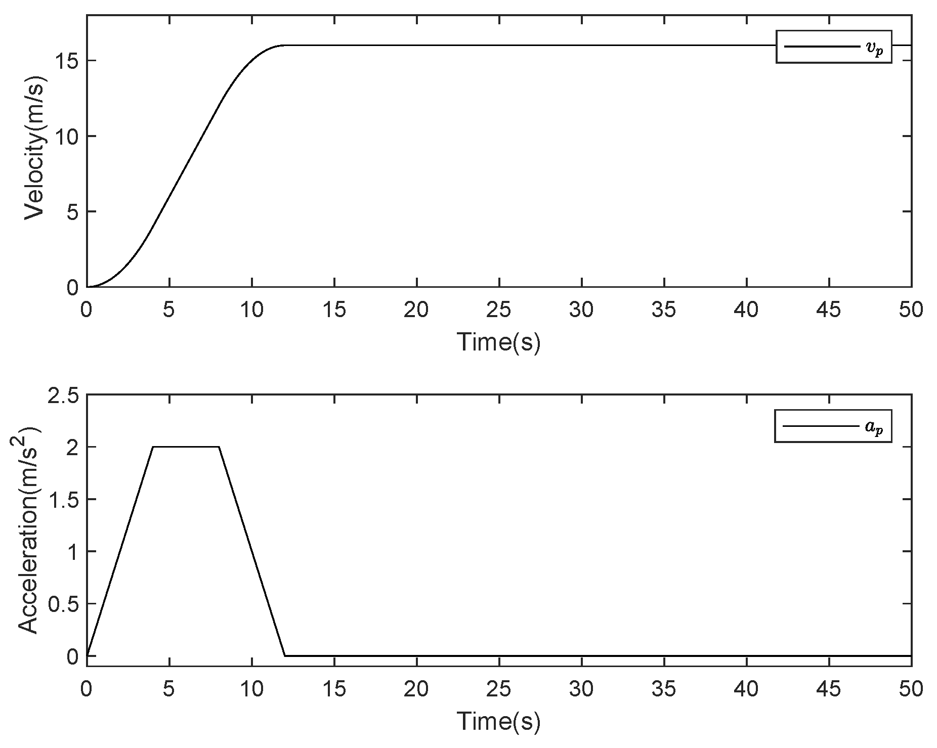
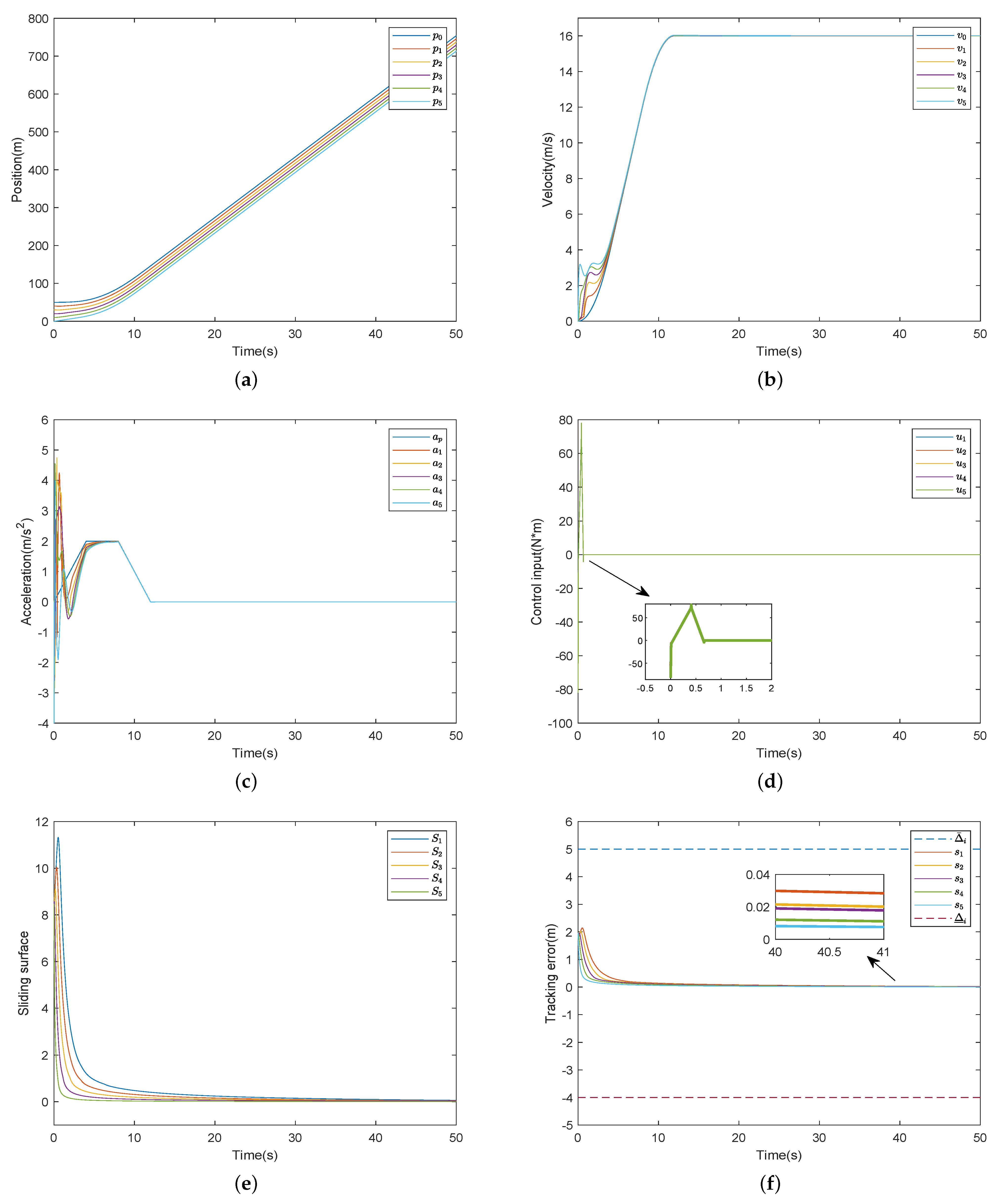
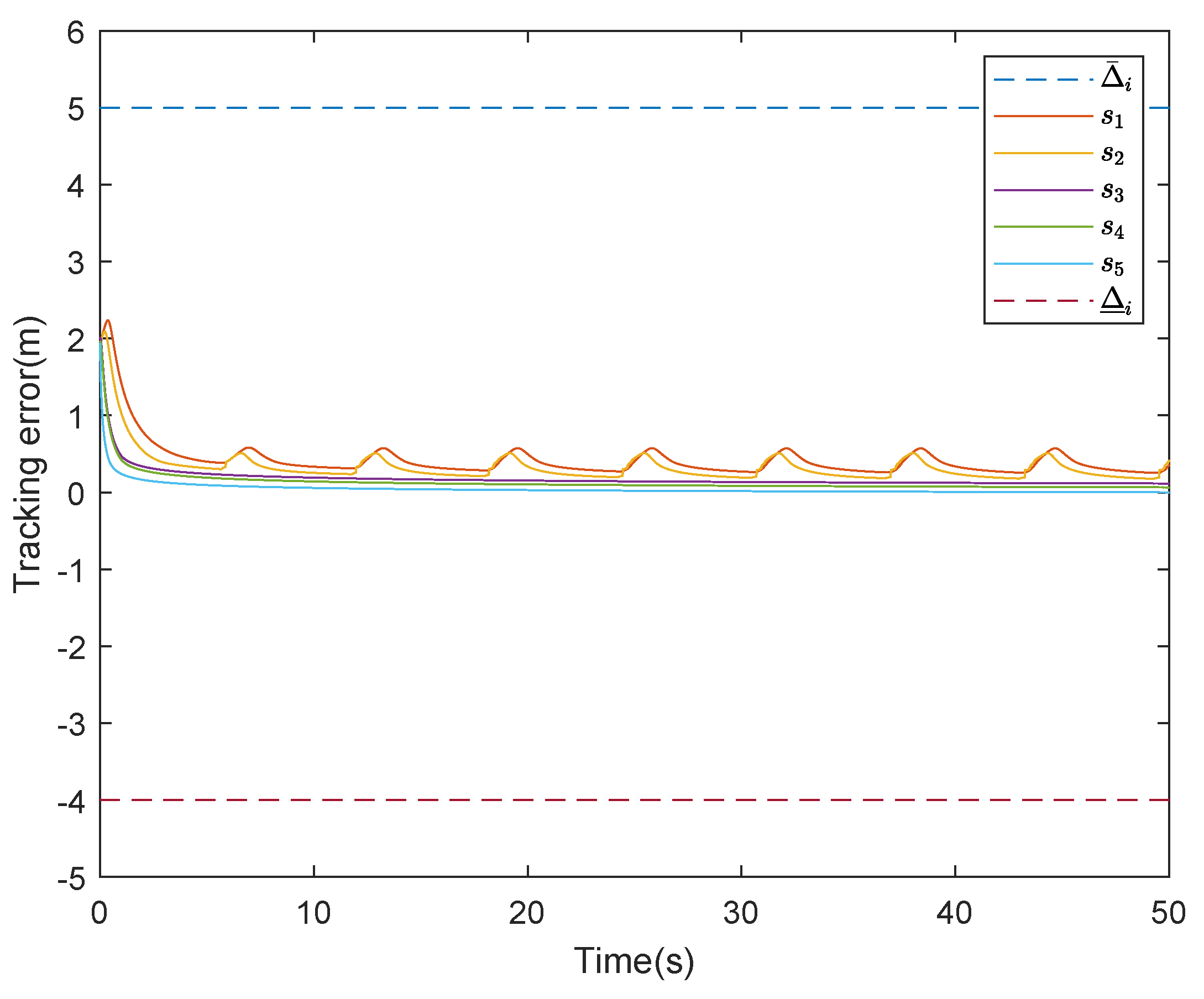
5. Simulation Studies

In the simulation, a platoon with five vehicles is considered, and the parameters of each vehicle are given in

Table 2. Model Parameters for Each Vehicle.

i	1	2	3	4	5
$m_i$ (kg)	1550	1450	1520	1510	1390
${\tau }_i$ (s)	0.15	0.25	0.32	0.41	0.35
${\rho }_{ai}$ (kg/m3)	1.2	1.2	1.2	1.2	1.2
$O_i$ (m2)	2.2	2.2	2.2	2.2	2.2
$C_{ai}$	0.414	0.414	0.414	0.414	0.414
${\Xi }_i$ (N)	236.2	236.2	236.2	236.2	236.2
$L_i$ (m)	4	4	4	4	4

. The desired distance between two adjacent vehicles is ${\Delta }_{i-1,i}=5\mathrm{m}$, the minimum safety distance is ${\Delta }_{col}=1\mathrm{m}$, the maximum effective communication distance is ${\Delta }_{con}=10\mathrm{m}$, the bias constraint function is ${\Delta }_{bc}=-0.5$, and the prescribed constraint function is $b_{c,i}$ = 4.5. The specific trajectories of the virtual leader are given in Figure 2 with $p_0\left(0\right)=50\mathrm{m}$, and the initial positions and velocities of the vehicles in the platoon are chosen as follows: $p_i\left(0\right)=[40,30,20,10,0]$, and $v_i\left(0\right)=0$ with zero initial tracking errors. The external disturbances are ${\omega }_i\left(t\right)=0.01sin\left(t\right)$, and the controller parameters are listed in

Table 3. Control Parameters of Each Vehicle.

$k_{1i}$	$k_{2i}$	$k_{3i}$	${\lambda }_{1i}$	${\lambda }_{2i}$	${\gamma }_i$	${\nu }_{1i}$	${\nu }_{2i}$	$h_i$
0.1	0.1	0.1	800	5000	0.9	3/7	5/3	0.2
${\Delta }_{i-1,i}$	${\iota }_i$	$g_i$	$b_i$	$c_i$	${\lambda }_i$	$k_{b,i}$	${\sigma }_{{\theta }_i}$	${\sigma }_{{\eta }_i}$
5	0.001	2	0.01	10	1	10	0.0001	0.0001

.

5.1. The Results of the Proposed Control Scheme without Actuator Faults

In this section, actuator faults are not considered, so the fault efficiency factor ${\rho }_i(t,t_{\rho ,i})$ and the bias fault $r_i(t,t_{r,i})$ are given as: ${\rho }_i(t,t_{\rho ,i})=1$, $r_i(t,t_{r,i})=0$, and $(i\in 1,2,\cdots ,5)$.

Figure 3 shows the simulation results, which illustrate that better control performance can be obtained under the proposed control scheme (i.e., Theorem 1 and 2) in this paper. Figure 3a–c show the position, velocity and acceleration of each vehicle, from which it is obvious that all the followers can follow the speed and acceleration of the virtual leader, while ensuring that the distance constraint is not violated. Figure 3d and Figure 3e describe the control input of the vehicles and sliding mode surfaces, respectively. From Figure 3f, it can be seen that the tracking error converges to a small region near zero in a fixed time under the effect of the proposed method, that is, individual vehicle stability is ensured. In addition, string stability can also be guaranteed, i.e., $\left|s_5\right|\le \left|s_4\right|\le \cdots \le \left|s_1\right|$. In conclusion, the given scheme is effective for the platoon system under distance constraints without actuator faults.

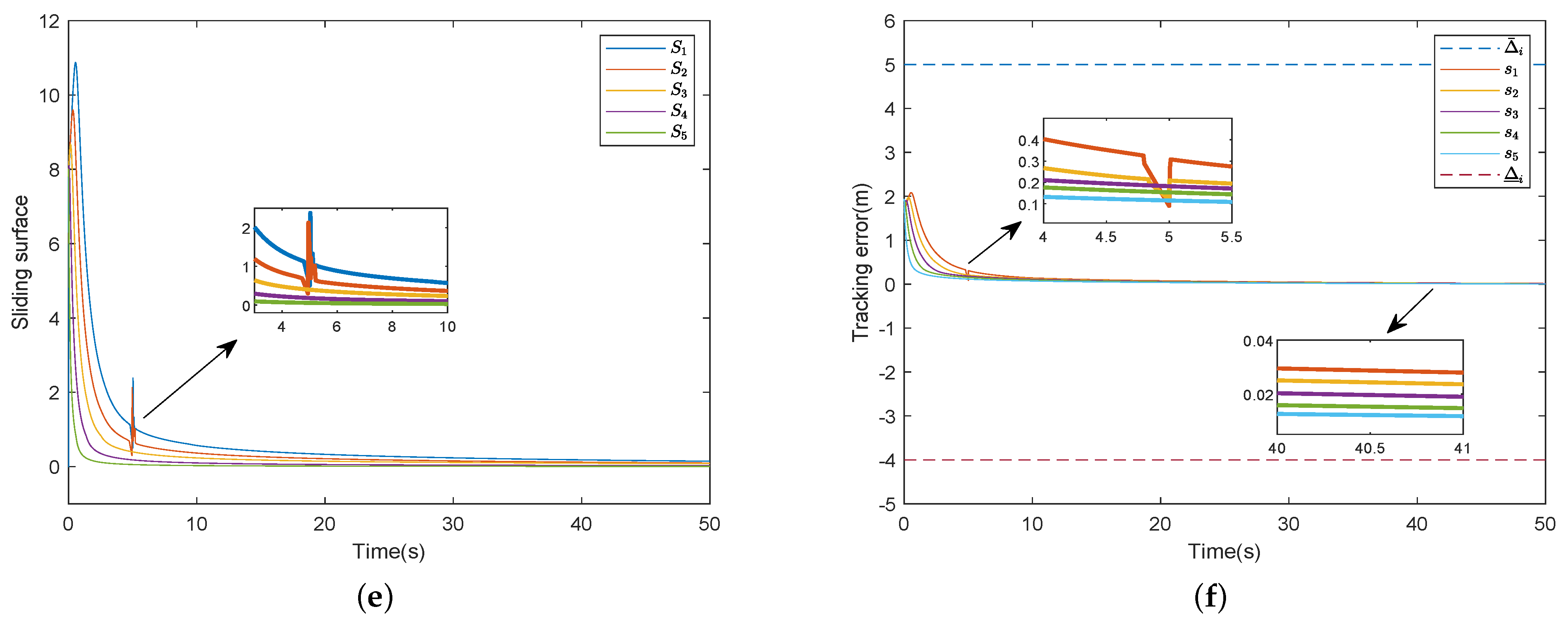
5.2. The Effect of Unknown Actuator Fault Directions

Case 1: (With the Nussbaum function). To account for actuator faults with unknown directions, we randomly set the fault efficiency factor ${\rho }_i(t,t_{\rho ,i})$ and bias fault $r_i(t,t_{r,i})$ to make the system more aligned with reality:

$$\begin{array}{c}\hfill \left\{\begin{array}{c}{\rho }_1(t,t_{\rho ,1})=-1.3-0.3cos\left(t\right),\hfill \\ {\rho }_2(t,t_{\rho ,2})=-0.5-0.3cos\left(t\right)\hfill \\ {\rho }_3(t,t_{\rho ,3})=1-0.3cos\left(t\right),\hfill \\ {\rho }_4(t,t_{\rho ,4})=0.5+0.3cos\left(t\right),\hfill \\ {\rho }_5(t,t_{\rho ,5})=1.3+0.3sin\left(t\right),\hfill \\ r_i(t,t_{r,i})=0.2+0.1cos\left(t\right).\hfill \end{array}\right.\end{array}$$

(63)

The results of Case 1 are shown in Figure 4. It is obvious that the platoon control is also achieved under the given control scheme. Note that when the direction of the fault is unknown, the impact of a reverse fault on the vehicle is more pronounced. As shown in Figure 4f, the tracking errors $s_1\left(t\right)$$s_2\left(t\right)$ appear as reverse faults around $5s$, the acceleration curves in Figure 4c, the control input in Figure 4d, and the sliding surface in Figure 4e also have peaks but quickly converge to near zero, and ensure system stability, string stability and collision avoidance, which show the effectiveness of the method proposed in Theorems 1 and 2.

Case 2: (Without the Nussbaum function). In this part, to further illustrate the effectiveness of the given method, a control scheme without the Nussbaum function is considered. The simulation result is shown in Figure 5. It shows the tracking error curve for the control scheme that does not handle actuator faults with unknown directions. The tracking error $s_i\left(t\right)$ is within the set constraints, but the curve keeps oscillating and the system becomes unstable. These all illustrate the necessity and advantages of the control scheme proposed in this paper.

In summary, the effectiveness of the proposed control scheme is well demonstrated, i.e., individual vehicle stability and string stability can be guaranteed in the conditions of time-varying actuator faults, uncertain parameters and unknown disturbances.

6. Conclusions

In this paper, fault-tolerant control of vehicle platoons with time-varying actuator fault directions and distance constraints is investigated. A novel Nussbaum function is introduced to handle unknown time-varying actuator fault directions. By incorporating a bias constraint function to modify the distance constraints, a new BLF mechanism is proposed, with which symmetric and asymmetric distance constraints can all be dealt with under the same framework. Further, a fixed-time fault-tolerant vehicle platoon control scheme is given, capable of guaranteeing individual vehicle stability and string stability within a fixed time.

References

1. Chu, S.; Majumdar, A. Opportunities and challenges for a sustainable energy future. Nature 2012, 488, 294–303. [Google Scholar] [CrossRef] [PubMed]
2. Zheng, Y.; Li, S.E.; Li, K.; Wang, L. Stability margin improvement of vehicular platoon considering undirected topology and asymmetric control. IEEE Trans. Control Syst. Technol. 2016, 24, 1253–1265. [Google Scholar] [CrossRef]
3. Ge, X.; Han, Q.-L.; Wang, J.; Zhang, X.M. A scalable adaptive approach to multi-vehicle formation control with obstacle avoidance. IEEE/CAA J. Autom. Sin. 2022, 9, 990–1004. [Google Scholar] [CrossRef]
4. Rödönyi, G. An adaptive spacing policy guaranteeing string stability in multi-brand ad hoc platoons. IEEE Trans. Intell. Transp. Syst. 2018, 19, 1902–1912. [Google Scholar] [CrossRef]
5. Wang, J.; Luo, X.; Wong, C.; Guan, X. Specified-time vehicular platoon control with flexible safe distance constraint. IEEE Trans. Veh. Technol. 2019, 68, 10489–10503. [Google Scholar] [CrossRef]
6. Zhou, Z.; Zhu, F.; Xu, D.; Guo, S.; Dai, Y. Event-triggered multi-lane fusion control for 2-D vehicle platoon systems with distance constraints. IEEE Trans. Intell. Veh. 2023, 8, 1498–1511. [Google Scholar] [CrossRef]
7. Guo, G.; Li, D. Adaptive sliding mode control of vehicular platoons with prescribed tracking performance. IEEE Trans. Veh. Technol. 2019, 68, 7511–7520. [Google Scholar] [CrossRef]
8. Guo, X.; Wang, J.; Liao, F.; Teo, R.S.H. Distributed adaptive integrated-sliding-mode controller synthesis for string stability of vehicle platoons. IEEE Trans. Intell. Transp. Syst. 2016, 17, 2419–2429. [Google Scholar] [CrossRef]
9. Guo, X.G.; Xu, W.D.; Wang, J.L.; Park, J.H.; Yan, H. BLF-based neuroadaptive fault-tolerant control for nonlinear vehicular platoon with time-varying fault directions and distance restrictions. IEEE Trans. Intell. Transp. Syst. 2022, 23, 12388–12398. [Google Scholar] [CrossRef]
10. Aaron, D.; Xu, X.; Grizzle, W.; Tabuada, P. Control barrier function based quadratic programs for safety critical systems. IEEE Trans. Autom. Control 2017, 62, 3861–3876. [Google Scholar]
11. Wu, Z.; Albalawi, F.; Zhang, Z.; Zhang, J.; Durand, H.; Panagiotis, D. Control Lyapunov-barrier function-based model predictive control of nonlinear systems. Automatica 2019, 109, 108508. [Google Scholar] [CrossRef]
12. Wei, H.; Liu, J.; Chen, H.; Liu, L. Fuzzy adaptive control for vehicular platoons with constraints and unknown dead-zone input. IEEE Trans. Intell. Transp. Syst. 2023, 24, 4403–4412. [Google Scholar] [CrossRef]
13. Lei, Y.; Li, X.; Tong, C. Distributed adaptive asymptotic tracking of 2-D vehicular platoon systems with actuator faults and spacing constraints. IEEE/CAA J. Autom. Sin. 2023, 10, 1352–1354. [Google Scholar] [CrossRef]
14. Guo, X.G.; Xu, W.D.; Wang, J.L.; Park, J.H. Distributed neuroadaptive fault-tolerant sliding-mode control for 2-D plane vehicular platoon systems with spacing constraints and unknown direction faults. Automatica 2021, 129, 109–675. [Google Scholar] [CrossRef]
15. Li, L.; Luo, H.; Ding, X.; Yang, Y.; Peng, X. Performance-based fault detection and fault-tolerant control for automatic control systems. Automatica 2019, 99, 308–316. [Google Scholar] [CrossRef]
16. Xiao, Y.; Dong, X. Distributed fault-tolerant containment control for nonlinear multi-agent systems under directed network topology via hierarchical approach. IEEE/CAA J. Autom. Sin. 2021, 8, 806–816. [Google Scholar] [CrossRef]
17. Pan, C.; Chen, Y.; Liu, Y.; Ali, I. Adaptive resilient control for interconnected vehicular platoon with fault and saturation. IEEE Trans. Intell. Transp. Syst. 2022, 23, 10210–10222. [Google Scholar] [CrossRef]
18. Guo, G.; Li, P.; Hao, L.Y. A new quadratic spacing policy and adaptive fault-tolerant platooning with actuator saturation. IEEE Trans. Intell. Transp. Syst. 2022, 23, 1200–1212. [Google Scholar] [CrossRef]
19. Gao, Z.Y.; Zhang, Y.; Guo, G. Finite-time fault-tolerant prescribed performance control of connected vehicles with actuator saturation. IEEE Trans. Veh. Technol. 2023, 72, 1438–1448. [Google Scholar] [CrossRef]
20. Sun, Y.; Wang, F.; Liu, Z.; Zhang, Y.; Chen, C.L.P. Fixed-time fuzzy control for a class of nonlinear systems. IEEE Trans. Cybern. 2022, 52, 3880–3887. [Google Scholar] [CrossRef]
21. Yang, H.; Ye, D. Adaptive fixed-time bipartite tracking consensus control for unknown nonlinear multi-agent systems: An information classification mechanism. Inf. Sci. 2018, 459, 238–254. [Google Scholar] [CrossRef]
22. Zuo, Z. Nonsingular fixed-time consensus tracking for second-order multi-agent networks. Automatica 2015, 54, 305–309. [Google Scholar] [CrossRef]
23. Ren, B.; Ge, S.S.; Tee, K.P.; Lee, T.H. Adaptive neural control for output feedback nonlinear systems using a barrier Lyapunov function. IEEE Trans. Neural Netw. 2010, 21, 1339–1345. [Google Scholar] [PubMed]
24. Shahvali, M.; Shojaei, K. Distributed adaptive neural control of nonlinear multi-agent systems with unknown control directions. Nonlinear Dyn. 2016, 83, 2213–2228. [Google Scholar] [CrossRef]
25. Li, D.; Guo, G. Prescribed performance concurrent control of connected vehicles with nonlinear third-order dynamics. IEEE Trans. Veh. Technol. 2020, 69, 14793–14802. [Google Scholar] [CrossRef]
26. Kwon, J.W.; Chwa, D. Adaptive bidirectional platoon control using a coupled sliding mode control method. IEEE Trans. Intell. Transp. Syst. 2014, 15, 2040–2048. [Google Scholar] [CrossRef]
27. Gao, Z.; Zhang, Y.; Guo, G. Adaptive fixed-time prescribed performance control of vehicular platoons with unknown dead-zone and actuator saturation. Int. J. Robust Nonlinear Control 2023, 33, 1231–1253. [Google Scholar] [CrossRef]
Figure 1. The interaction structure of a vehicular platoon with a virtual leader.
Mathematics 12 02560 g001
Figure 2. Profile of the platoon velocity and acceleration.
Mathematics 12 02560 g002
Figure 3. Simulation results without faults. (a) Position. (b) Velocity. (c) Acceleration. (d) Control input. (e) Sliding surface. (f) Tracking error.
Mathematics 12 02560 g003
Figure 4. Simulation results in Case 1. (a) Position. (b) Velocity. (c) Acceleration. (d) Control input. (e) Sliding surface. (f) Tracking error.
Mathematics 12 02560 g004aMathematics 12 02560 g004b
Figure 5. The tracking error without the Nussbaum function.
Mathematics 12 02560 g005