

Robust Overbooking for No-Shows and Cancellations in Healthcare


Abstract
:1. Introduction
2. Background
3. Literature Review
4. Proposed Model
4.1. Basic Model
- Determining the number of consultation rooms to open on any given day;
- Assigning appointments to each consultation room.
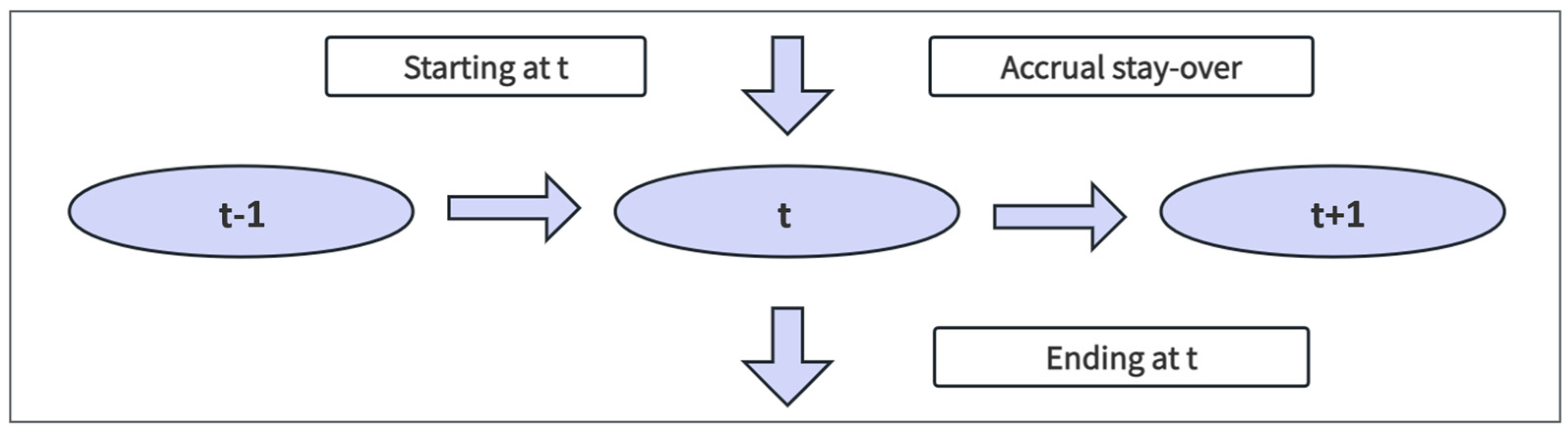
4.2. Preliminary Foundation
4.3. The Proposed Approach
4.4. Robust Optimization Model
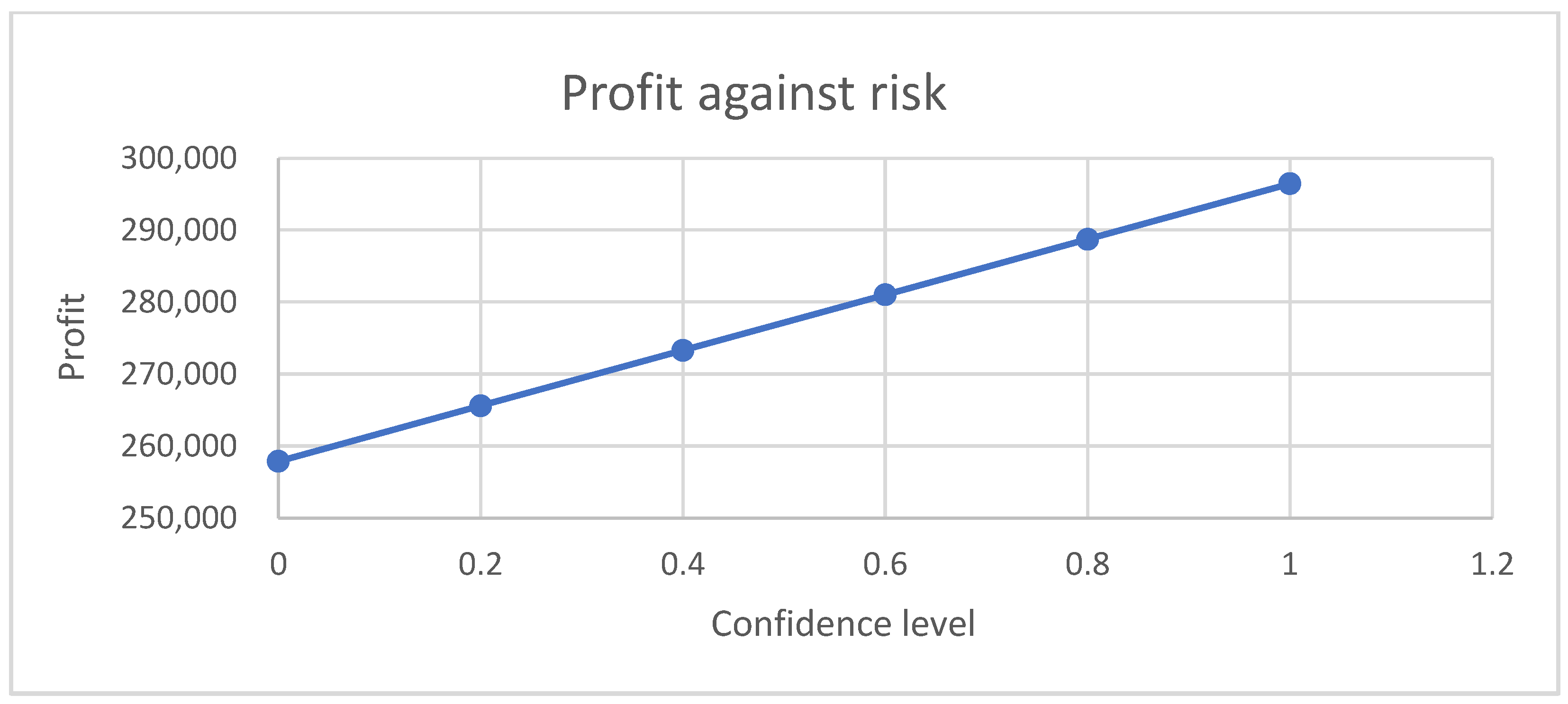
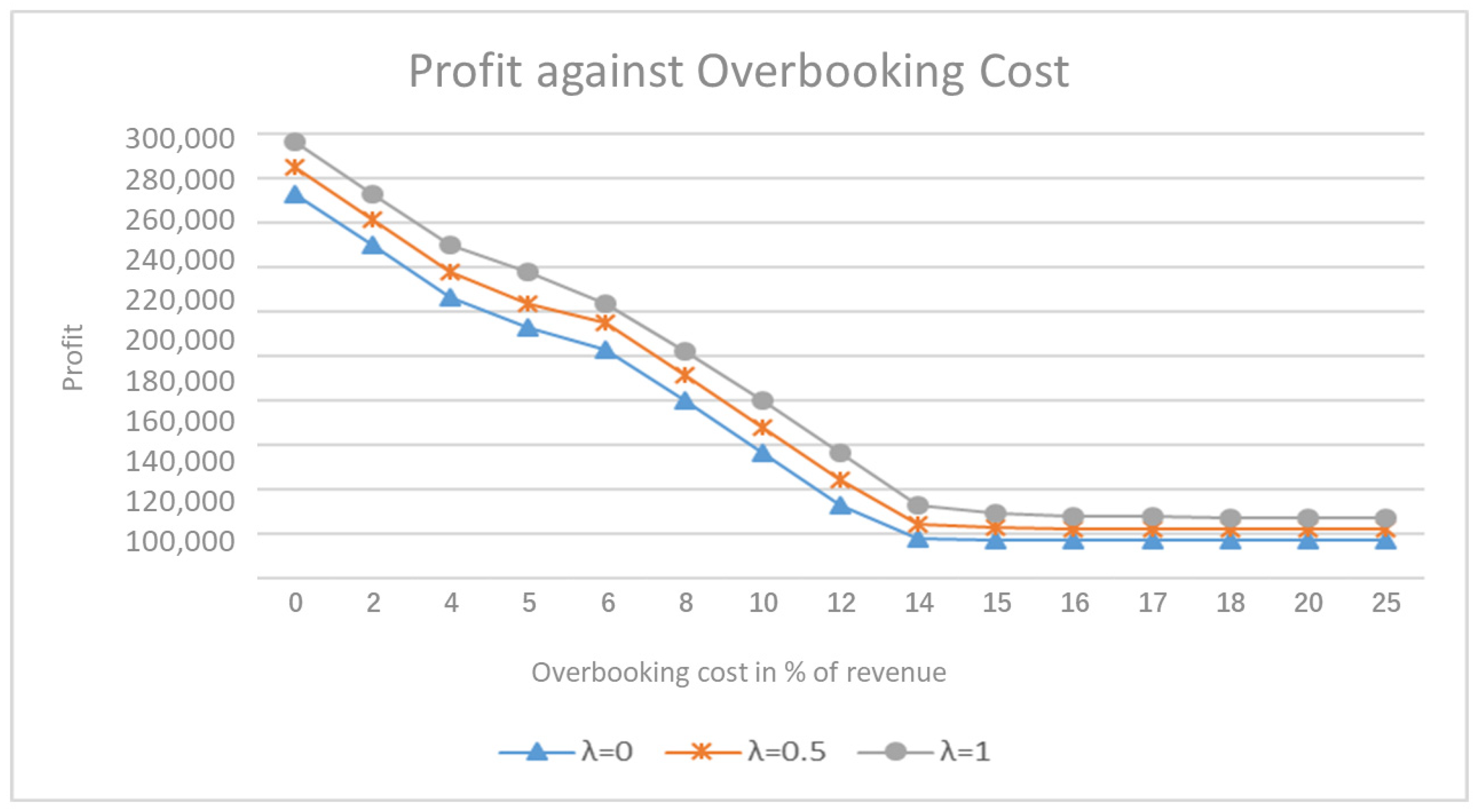
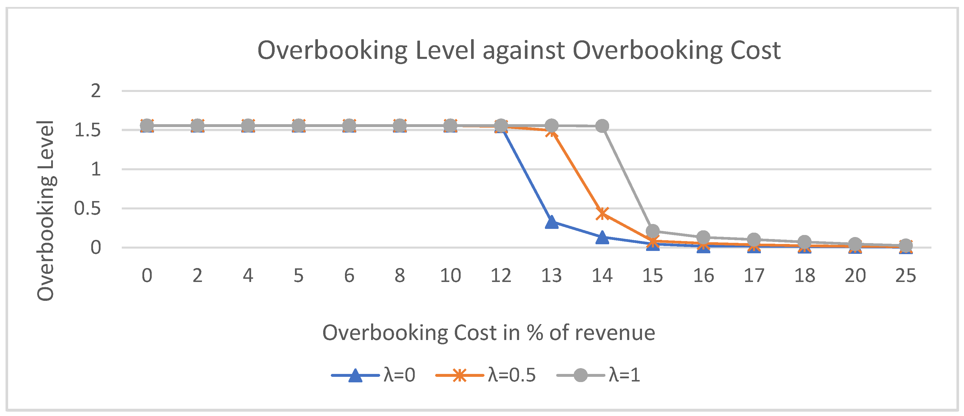
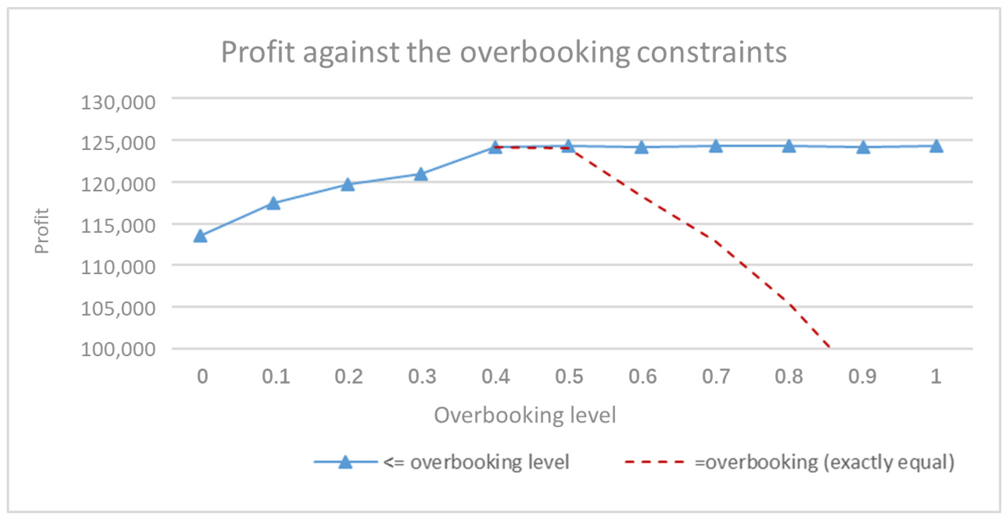
5. Result and Discussion
- The number of departments and their capacities cannot be expanded quickly.
- The revenue generated from each appointment is likely fixed in accordance with the policy of the Hong Kong Hospital Authority.
- The probability of patients attending their scheduled appointments remains constant.
- Demand is consistently high and exceeds capacity, making overbooking advantageous.
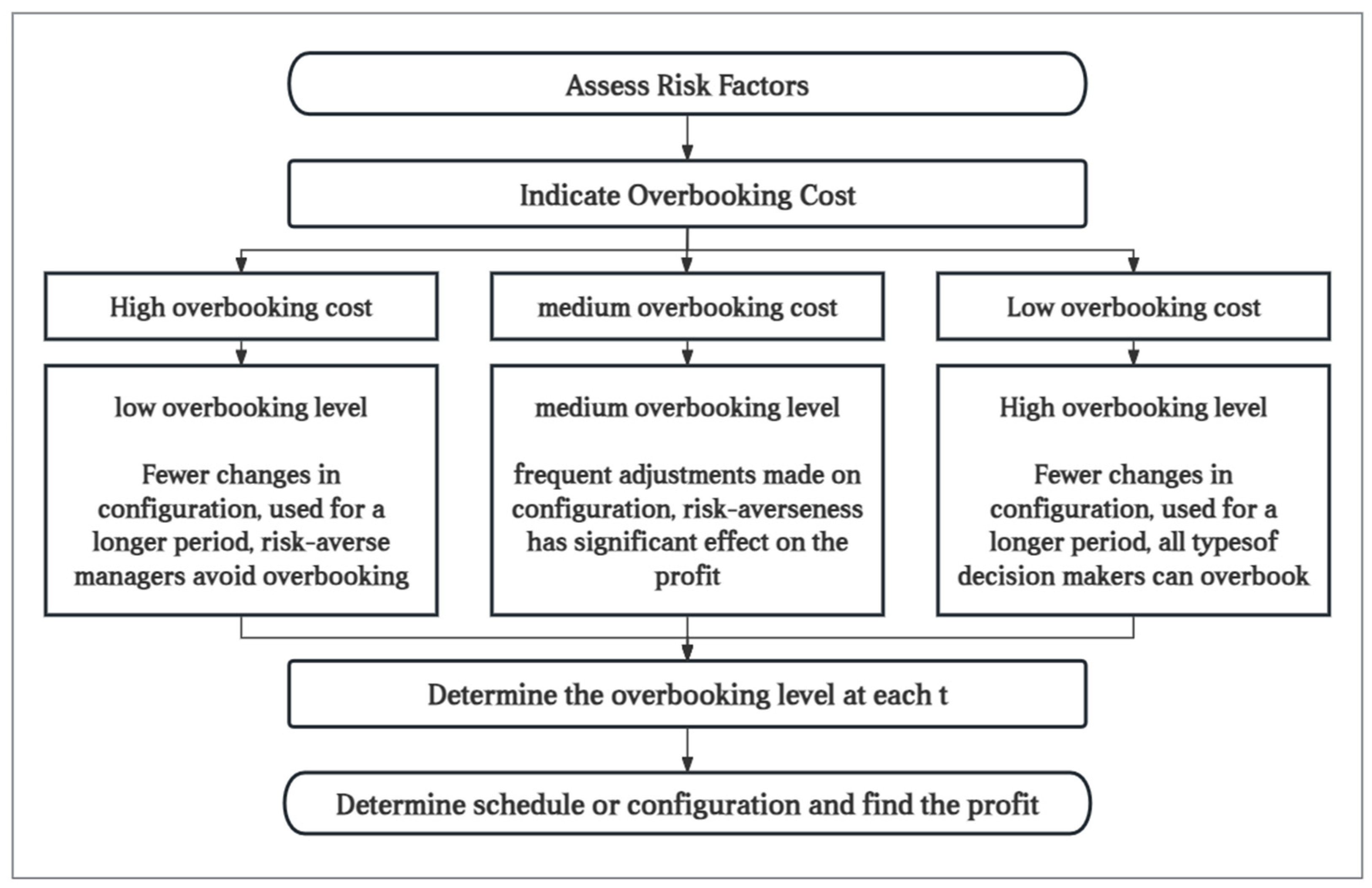
6. Management Insights
7. Superiority and Inferiority of the Proposed Optimization Strategy
8. Conclusions
Author Contributions
Funding
Data Availability Statement
Acknowledgments
Conflicts of Interest
References
- Haldane, V.; De Foo, C.; Abdalla, S.M.; Jung, A.; Tan, M.; Wu, S.; Chua, A.; Verma, M.; Shrestha, P.; Singh, S.; et al. Health systems resilience in managing the COVID-19 pandemic: Lessons from 28 countries. Nat. Med. 2021, 27, 964–980. [Google Scholar] [CrossRef] [PubMed]
- Riyapan, S.; Chantanakomes, J.; Roongsaenthong, P.; Tianwibool, P.; Wittayachamnankul, B.; Supasaovapak, J.; Pansiritanachot, W. Impact of the COVID-19 outbreak on out-of-hospital cardiac arrest management and outcomes in a low-resource emergency medical service system: A perspective from Thailand. Int. J. Emerg. Med. 2022, 15, 26. [Google Scholar] [CrossRef] [PubMed]
- Makridakis, S.; Kirkham, R.; Wakefield, A.; Papadaki, M.; Kirkham, J.; Long, L. Forecasting, uncertainty and risk; perspectives on clinical decision-making in preventive and curative medicine. Int. J. Forecast. 2019, 35, 659–666. [Google Scholar] [CrossRef]
- Weil, D.N. Accounting for the effect of health on economic growth. Q. J. Econ. 2007, 122, 1265–1306. [Google Scholar] [CrossRef]
- Odrakiewicz, D. The connection between health and economic growth: Policy implications re-examined. Glob. Manag. J. 2012, 4, 65–76. [Google Scholar]
- White, D.L.; Froehle, C.M.; Klassen, K.J. The effect of integrated scheduling and capacity policies on clinical efficiency. Prod. Oper. Manag. 2011, 20, 442–455. [Google Scholar] [CrossRef]
- Klassen, K.J.; Yoogalingam, R. Appointment scheduling in multi-stage outpatient clinics. Health Care Manag. Sc. 2018, 22, 229–244. [Google Scholar] [CrossRef]
- Srinivas, S.; Ravindran, A.R. Designing schedule configuration of a hybrid appointment system for a two-stage outpatient clinic with multiple servers. Health Care Manag. Sci. 2020, 23, 360–386. [Google Scholar] [CrossRef] [PubMed]
- Mitchell, A.J.; Selmes, T. Why don’t patients attend their appointments? Maintaining engagement with psychiatric services. Adv. Psychiatr. Treat. 2007, 13, 423–434. [Google Scholar] [CrossRef]
- Sweetman, S.; Sharkey, A.R.; Thomas, K.; Dhesi, J. Reduction of last-minute cancellations in elective urology surgery: A quality improvement study. Int. J. Surg. 2020, 74, 29–33. [Google Scholar] [CrossRef] [PubMed]
- Lan, Y.; Ball, M.O.; Karaesmen, I.Z.; Zhang, J.X.; Liu, G.X. Analysis of seat allocation and overbooking decisions with hybrid information. Eur. J. Oper. Res. 2014, 240, 493–504. [Google Scholar] [CrossRef]
- He, W. Integrating overbooking with capacity planning: Static model and application to airlines. Prod. Oper. Manag. 2019, 28, 1972–1989. [Google Scholar] [CrossRef]
- Pimentel, V.; Aizezikali, A.; Baker, T. Hotel revenue management: Benefits of simultaneous overbooking and allocation problem formulation in price optimization. Comput. Ind. Eng. 2019, 137, 106073. [Google Scholar] [CrossRef]
- Kuiper, A.; Mandjes, M.; de Mast, J.; Brokkelkamp, R. A flexible and optimal approach for appointment scheduling in healthcare. Decis. Sci. 2021, 54, 85–100. [Google Scholar] [CrossRef]
- Gupta, D.; Denton, B. Appointment scheduling in health care: Challenges and opportunities. IIE Trans. 2008, 40, 800–819. [Google Scholar] [CrossRef]
- Stanciu, A.; Vargas, L.; May, J. A revenue management approach for managing operating room capacity. In Proceedings of the WSC10: Winter Simulation Conference, Baltimore, MD, USA, 5–8 December 2010; pp. 2444–2454. [Google Scholar]
- Ratcliffe, A.; Gilland, W.; Marucheck, A. Revenue management for outpatient appointments: Joint capacity control and overbooking with class-dependent no-shows. Flex. Serv. Manuf. J. 2011, 24, 516–548. [Google Scholar] [CrossRef]
- Roski, J.; Gregory, R. Performance measurement for ambulatory care: Moving towards a new agenda. Int. J. Qual. Health C 2001, 13, 447–453. [Google Scholar] [CrossRef] [PubMed]
- Subramanian, J.; Stidham, S.; Lautenbacher, C.J. Airline yield management with overbooking, cancellations, and no-shows. Transp. Sci. 1999, 33, 147–167. [Google Scholar] [CrossRef]
- Liberman, V.; Yechiali, U. On the hotel overbooking problem—An inventory system with stochastic cancellations. Manag. Sci. 1978, 24, 1117–1126. [Google Scholar] [CrossRef]
- Ho, C.; Lau, H. Minimizing total cost in scheduling outpatient appointments. Manag. Sci. 1992, 38, 1750–1764. [Google Scholar] [CrossRef]
- Kros, J.; Dellana, S.; West, D. Overbooking increases patient access at east carolina university’s student health services clinic. Interfaces 2009, 39, 271–287. [Google Scholar] [CrossRef]
- LaGanga, L.R.; Lawrence, S.R. Clinic overbooking to improve patient access and increase provider productivity. Decis. Sci. 2007, 38, 251–276. [Google Scholar] [CrossRef]
- Lee, D.K.K.; Zenios, S.A. Optimal capacity overbooking for the regular treatment of chronic conditions. Oper. Res. 2009, 57, 852–865. [Google Scholar] [CrossRef]
- Muthuraman, K.; Lawley, M. A stochastic overbooking model for outpatient clinical scheduling with no-shows. IIE Trans. 2008, 40, 820–837. [Google Scholar] [CrossRef]
- Sonnenberg, A. How to overbook procedures in the endoscopy unit. Gastrointest. Endosc. 2009, 69, 710–715. [Google Scholar] [CrossRef] [PubMed]
- Kazim, T.; Urban, T.L.; Russell, R.A.; Yildirim, M.B. Decision support system for appointment scheduling and overbooking under patient no-show behavior. Ann. Oper. Res. 2024. [Google Scholar] [CrossRef]
- Han, Y.; Johnson, M.E.; Shan, X.; Khasawneh, M. A multi—Appointment patient scheduling system with machine learning and optimization. Decis. Anal. J. 2024, 10, 100392. [Google Scholar] [CrossRef]
- Liu, N.; Ziya, S. Panel size and overbooking decisions for appointment-based services under patient no-shows. Prod. Oper. Manag. 2014, 23, 2209–2223. [Google Scholar] [CrossRef]
- Kim, S.; Giachetti, R.E. A stochastic mathematical appointment overbooking model for healthcare providers to improve profits. IEEE Trans. Syst. Man Cybern. Part A Syst. Hum. 2006, 36, 1211–1219. [Google Scholar] [CrossRef]
- LaGanga, L.R.; Lawrence, S.R. Appointment overbooking in health care clinics to improve patient service and clinic performance. Prod. Oper. Manag. 2012, 21, 874–888. [Google Scholar] [CrossRef]
- Kolisch, R.; Sickinger, S. Providing radiology health care services to stochastic demand of different customer classes. OR Spectr. 2007, 30, 375–395. [Google Scholar] [CrossRef]
- Zeng, B.; Turkcan, A.; Lin, J.; Lawley, M. Clinic scheduling models with overbooking for patients with heterogeneous no-show probabilities. Ann. Oper. Res. 2010, 178, 121–144. [Google Scholar] [CrossRef]
- Liu, N.; Ziya, S.; Kulkarni, V.G. Dynamic scheduling of outpatient appointments under patient no-shows and cancellations. Manuf. Serv. Oper. Manag. 2010, 12, 347–364. [Google Scholar] [CrossRef]
- Parizi, M.S.; Ghate, A. Multi-class, multi-resource advance scheduling with no-shows, cancellations and overbooking. Comput. Oper. Res. 2016, 67, 90–101. [Google Scholar] [CrossRef]
- Schütz, H.; Kolisch, R. Capacity allocation for demand of different customer-product-combinations with cancellations, no-shows, and overbooking when there is a sequential delivery of service. Ann. Oper. Res. 2013, 206, 401–423. [Google Scholar] [CrossRef]
- Bellini, V.; Russo, M.; Domenichetti, T.; Panizzi, M.; Allai, S.; Elena, G.B. Artificial intelligence in operating room management. J. Med. Syst. 2024, 48, 19. [Google Scholar] [CrossRef]
- Wang, W.Y.; Gupta, D. Adaptive appointment systems with patient preferences. Manuf. Serv. Oper. Manag. 2011, 13, 373–389. [Google Scholar] [CrossRef]
- Samorani, M.; LaGanga, L.R. Outpatient appointment scheduling given individual day-dependent no-show predictions. Eur. J. Oper. Res. 2015, 240, 245–257. [Google Scholar] [CrossRef]
- Bheemidi, A.R.; Kailar, R.; Valentim, C.C.S.; Kalur, A.; Singh, R.P.; Talcott, K.E. Baseline factors and reason for cancellation of elective ophthalmic surgery. Eye 2023, 2023, 2788–2794. [Google Scholar] [CrossRef]
- Cayirli, T.; Veral, E. Outpatient scheduling in health care: A review of literature. Prod. Oper. Manag. 2003, 12, 519–549. [Google Scholar] [CrossRef]
- Lai, K.K.; Wang, S.Y.; Xu, J.P.; Zhu, S.S.; Fang, Y. A class of linear interval programming problems and its application to portfolio selection. IEEE Trans. Fuzzy Syst. 2002, 10, 698–704. [Google Scholar] [CrossRef]
- Alefeld, G.; Herzberger, J. Introduction to Interval Computation, 1st ed.; Academic Press: Cambridge, MA, USA, 1983; pp. 1–49. [Google Scholar]
- Chankong, V.; Haimes, Y.Y. Multiobjective Decision Making: Theory and Methodology, 1st ed.; Courier Dover Publications: New York, NY, USA, 2008; pp. 291–322. [Google Scholar]
- Schrage, L. Optimization Modeling with LINDO, 5th ed.; LINDO Systems Inc.: Chicago, IL, USA, 2003; pp. 507–528. [Google Scholar]

| No. | Topics | Sources | Findings/Methodologies |
|---|---|---|---|
| 1 | Factors affecting no-show | [15,38,39,40,41] | Weather, physical distance, waiting time, appointment intervals, etc. |
| 2 | Impact of no-show | [34,35,36,37] | Waste of resources, reprogramming, harm to patient health, etc. |
| 3 | Effectiveness of overbooking | [22,23,24,25,26,29,31,32] | Maximize expected profits, reduce waiting times, optimize performance, etc. |
| 4 | Optimal overbooking strategy | [14,27,28,29,30] | Single-server queuing model, stochastic model, phase-type distributions, ML, ANNs, etc. |
| From/To | 1 | 2 | 3 | 4 | 5 | 6 |
|---|---|---|---|---|---|---|
| 0 | 60 | 21 | 28 | 30 | 25 | 35 |
| 1 | 30 | 28 | 35 | 25 | 21 | |
| 2 | 25 | 35 | 25 | 21 | ||
| 3 | 25 | 21 | 25 | |||
| 4 | 25 | 21 | ||||
| 5 | 25 |
| From/To | 1 | 2 | 3 | 4 | 5 | 6 |
|---|---|---|---|---|---|---|
| 0 | 120 | 42 | 55 | 60 | 50 | 70 |
| 1 | 60 | 55 | 70 | 50 | 42 | |
| 2 | 50 | 70 | 50 | 42 | ||
| 3 | 50 | 42 | 50 | |||
| 4 | 50 | 42 | ||||
| 5 | 50 |
| Denotation | ||||||
|---|---|---|---|---|---|---|
| Value | 100 | 0.8 | 0.95 | 500 | 10 | 10 |
| Overbooking | t = 1 | t = 2 | t = 3 | t = 4 | t = 5 |
|---|---|---|---|---|---|
| Specialty 1 | 200 | 198 | 196 | 200 | 198 |
| Specialty 2 | 199 | 200 | 198 | 200 | 200 |
| Specialty 3 | 200 | 200 | 200 | 197 | 199 |
| From/To, Specialty 1 | 1 | 2 | 3 | 4 | 5 | 6 |
|---|---|---|---|---|---|---|
| 0 | 90 | 31 | 41 | 45 | 37 | 51 |
| 1 | 16 | 12 | 18 | 20 | 31 | |
| 2 | 14 | 27 | 16 | 31 | ||
| 3 | 15 | 30 | 37 | |||
| 4 | 17 | 31 | ||||
| 5 | 37 | |||||
| Specialty 2 | ||||||
| 0 | 40 | 39 | 44 | 49 | 66 | 49 |
| 1 | 9 | 30 | 19 | 10 | 48 | |
| 2 | 8 | 26 | 4 | 41 | ||
| 3 | 7 | 25 | 45 | |||
| 4 | 7 | 52 | ||||
| 5 | 56 | |||||
| Specialty 3 | ||||||
| 0 | 39 | 37 | 41 | 46 | 63 | 50 |
| 1 | 5 | 45 | 15 | 17 | 47 | |
| 2 | 3 | 34 | 14 | 39 | ||
| 3 | 10 | 23 | 42 | |||
| 4 | 8 | 50 | ||||
| 5 | 54 |
Disclaimer/Publisher’s Note: The statements, opinions and data contained in all publications are solely those of the individual author(s) and contributor(s) and not of MDPI and/or the editor(s). MDPI and/or the editor(s) disclaim responsibility for any injury to people or property resulting from any ideas, methods, instructions or products referred to in the content. |
© 2024 by the authors. Licensee MDPI, Basel, Switzerland. This article is an open access article distributed under the terms and conditions of the Creative Commons Attribution (CC BY) license (https://creativecommons.org/licenses/by/4.0/).
Share and Cite
Xiao, F.; Lai, K.K.; Lau, C.K.; Ram, B. Robust Overbooking for No-Shows and Cancellations in Healthcare. Mathematics 2024, 12, 2563. https://doi.org/10.3390/math12162563
Xiao F, Lai KK, Lau CK, Ram B. Robust Overbooking for No-Shows and Cancellations in Healthcare. Mathematics. 2024; 12(16):2563. https://doi.org/10.3390/math12162563
Chicago/Turabian StyleXiao, Feng, Kin Keung Lai, Chun Kit Lau, and Bhagwat Ram. 2024. "Robust Overbooking for No-Shows and Cancellations in Healthcare" Mathematics 12, no. 16: 2563. https://doi.org/10.3390/math12162563
APA StyleXiao, F., Lai, K. K., Lau, C. K., & Ram, B. (2024). Robust Overbooking for No-Shows and Cancellations in Healthcare. Mathematics, 12(16), 2563. https://doi.org/10.3390/math12162563