Fibonacci Wavelet Collocation Method for Solving Dengue Fever SIR Model

Abstract

The main focus in this manuscript is to find a numerical solution of a dengue fever disease model by using the Fibonacci wavelet method. The operational matrix of integration has been obtained using Fibonacci wavelets. The proposed method is called Fibonacci wavelet collocation method (FWCM). This biological model has been transformed into a system of nonlinear algebraic equations by using the Fibonacci wavelet collocation scheme. Afterward, this system has been solved by using the Newton–Raphson method. Finally, we provide evidence that our results are better than those obtained by various current approaches, both numerically and graphically, demonstrating the method’s accuracy and efficiency.

1. Introduction

Mathematics plays an important role in the betterment of human life. To solve real-life problems, a mathematical model has been proved to be one of the powerful tools; for example, one can discuss the severity of a disease in a particular region by using models. Over the years, mathematicians have done a tremendous job of revealing biological models. Usually, various biological models can be expressed as a system of ordinary differential equations. Most of these biological models are complex in nature, and only a few of them have analytical solutions. Consequently, a reasonable approximate solution is required. Numerical approaches are usually the best option for these systems since they lead us to answers and characterize the dynamic behavior of such systems.

One of the most dangerous and common diseases transmitted, due to mosquitoes in the world, is dengue [1,2]. About 390 million new cases of dengue are reported in a year, 96 million of which are symptomatic, according to recent data [3,4]. Asia accounts for the majority of newly diagnosed cases each year (about 70% of 390 million cases), with infection distributions of roughly 16.4%, 13.8%, and 0.2% shared by Africa, the Americas, and Oceania, respectively [3]. Aedes albopictus and Aedes aegypti are the primary vectors that spread dengue [5]. There are four different but closely related serotypes of the Flavivirus genus known as dengue virus (DENV): DENV-1, DENV-2, DENV-3, and DENV-4. Homologous immunity refers to the fact that an individual infected with any one of the types will never become infected with the same type again. However, a person loses immunity to the other varieties within around 12 weeks of contracting any of the aforementioned types.

Dengue fever’s mathematical modeling is [6,7]

$$\begin{array}{cc}\hfill {\displaystyle \frac{dS\left(t\right)}{dt}}& ={\mu }_h(1-S\left(t\right))-\alpha S\left(t\right)R\left(t\right)\hfill \end{array}$$

(1)

$$\begin{array}{cc}\hfill {\displaystyle \frac{dI\left(t\right)}{dt}}& =\alpha S\left(t\right)R\left(t\right)-\beta I\left(t\right)\hfill \end{array}$$

(2)

$$\begin{array}{cc}\hfill {\displaystyle \frac{dR\left(t\right)}{dt}}& =\gamma (1-R(t\left)\right)I\left(t\right)-\delta R\left(t\right)\hfill \end{array}$$

(3)

where $S\left(t\right)$ is the susceptible population (potential victims), $I\left(t\right)$ is the infected population, $R\left(t\right)$ represents recovered population from dengue at time $\left(t\right)$, ${\mu }_h$ is the natural death rate of the human population, $\alpha$ is the vaccine efficiency coefficient, $\delta$ is the number of deaths among the susceptible population, $\gamma$ is the recovery rate, and $\beta$ is the rate of infection in the human population. This model is a variation of the classical SIR (Susceptible–Infected–Recovered) model. Over the years, various numerical techniques have been applied by researchers for the SIR model of dengue fever, and few of them are as follows: M. Khalid et al. [8] proposed a new approach called the Perturbation Iteration Algorithm (PIM), Rangkuti et al. [9] implemented the Homotopy Perturbation Method and Variational Iteration method, Mungkasi [10] recommended an Improved Variational Iteration Method for the SIR model of dengue, Umar et al. [11] established a stochastic numerical computing scheme with artificial neural networks, Lede et al. [12] presented Euler and Heun methods, and Fei et al. [13] suggested a numerical collocation method using Bernoulli wavelets (BWCM).

Wavelet techniques emerged in the mid-1980s, drawing inspiration from concepts in both applied and pure mathematics. Based on an analysis function, Joseph Fourier created a technique in 1807 for expressing signals with a set of coefficients. He established the mathematical foundation on which the wavelet theory was created. Alfred Haar made the initial reference to wavelets in his doctoral dissertation in 1909. Currently, wavelet techniques have emerged as an effective approach for solving differential equations. Wavelet-based approaches are the most popular among scientists and engineers because of their smoothness, good localization, acceptability, and orthonormality. The wavelet theory has been an area of extensive research during the last 20 years. Numerous types of nonlinear differential equations have been solved by researchers using Haar, Legendre, and Chebyshev wavelets [14]. Other wavelets that have gained popularity among researchers include the Taylor wavelets [15], Müntz wavelets [16], Bernoulli wavelets [17], CAS wavelets [18], and Jacobi wavelets [19]. Specifically, wavelet-based collocation techniques have become popular in the field of numerical analysis, basically due to their straightforward methodology, easy computation, and fast convergence. It is important to note that different wavelet families, such as the Haar, Legendre, Chebyshev, Bernoulli, Euler, Hermite, Gegenbauer, and Fibonacci wavelets, have been used to solve a wide range of linear and nonlinear differential equations.

In the light of the interesting features and numerous advantages of wavelet-based numerical techniques over other currently used numerical methods, we are highly motivated to solve the Dengue Fever SIR model using the Fibonacci wavelet collocation method (FWCM). As far as we are aware, this wavelet technique has not yet been implemented for obtaining numerical solutions in the case of the dengue model. We make use of this to provide a novel numerical approach to discuss the above model based on compactly supported Fibonacci wavelets.

An overview of this article is as follows: Section 2 includes some basic definitions used throughout this article. Section 3 contains details about function approximation by Fibonacci wavelets. Section 4 is devoted to the construction of the operational matrix of integration based on Fibonacci wavelets for different values of M. Section 5 deals with the solution of the Dengue Fever SIR model by the proposed method. In Section 6, we state some theorems on Error Analysis. A comparison of solutions and Error Analysis through graphs and tables is shown in Section 7. This paper ends with a conclusion in Section 8.

2. Fundamental Definitions

In 1982, a French geophysical engineer, Jean Morlet, introduced the idea of a wavelet transform that provides a new mathematical procedure for seismic wave investigation [20]. A family of functions ${\psi }_{a,b}$ constructed by the translation and dilation of a single function $\psi$ (the mother wavelet) is called wavelet, as follows:

$$\begin{array}{c}\hfill {\psi }_{a,b}\left(x\right)={\displaystyle \frac{1}{\sqrt{\left|a\right|}}}\psi \left({\displaystyle \frac{x-b}{a}}\right),a,b\in \mathbb{R},a\ne 0\end{array}$$

(4)

where a and b are the dilation and translation parameters, respectively [21].

2.1. Fibonacci Polynomials

The following general formula is used to define Fibonacci polynomials [22], as follows:

$$\begin{array}{c}\hfill F_n\left(x\right)=\left\{\begin{array}{cc}1,\hfill & n=0,\hfill \\ x,\hfill & n=1,\hfill \\ x{F}_{n-1}\left(x\right)+F_{n-2}\left(x\right),\hfill & n>1.\hfill \end{array}\right.\end{array}$$

(5)

Furthermore, the power form of these polynomials is as follows [22]:

$$\begin{array}{cc}\hfill F_n\left(x\right)& {\displaystyle =\sum _{i=0}^{\lfloor \frac{n}{2}\rfloor }\left(\genfrac{}{}{0pt}{}{n-i}{i}\right)x^{n-2i},n\ge 0.}\hfill \end{array}$$

(6)

2.2. Fibonacci Wavelets

Fibonacci wavelets are defined on [0, 1] as follows [23]:

$$\begin{array}{c}\hfill {\psi }_{n,m}\left(x\right)=\left\{\begin{array}{cc}{\displaystyle \frac{1}{\sqrt{w_m}}}{2}^{(k-1)/2}{F}_m(2^{k-1}x-n+1),\hfill & {\displaystyle \frac{n-1}{2^{k-1}}}\le x<{\displaystyle \frac{n}{2^{k-1}}}\hfill \\ 0,\hfill & \mathrm{otherwise},\hfill \end{array}\right.\end{array}$$

(7)

with

$$\begin{array}{cc}\hfill w_m=& {\int }_0^1{F}_m^2\left(x\right)dx,\hfill \end{array}$$

(8)

where $m=0,1,\dots ,M-1$ is the degree of the Fibonacci polynomial $F_m\left(x\right)$, and $k=1,2,\dots$ and $n=1,2,\dots ,2^{k-1}$ denote the levels of the resolution and translation parameters, respectively. The coefficient ${\displaystyle \frac{1}{\sqrt{w_m}}}$ is referred to as normalization factor.

For example, for $k=1$ and $M=10$, we have Fibonacci wavelets as

$$\begin{array}{c}\hfill \begin{array}{cc}\hfill & {\psi }_{1,0}\left(x\right)=\left\{\begin{array}{cc}1,\hfill & 0\le x<1\hfill \\ 0,\hfill & \mathrm{otherwise}\hfill \end{array}\right.\hfill \\ \hfill & {\psi }_{1,1}\left(x\right)=\left\{\begin{array}{cc}\sqrt{3}x,\hfill & 0\le x<1\hfill \\ 0,\hfill & \mathrm{otherwise}\hfill \end{array}\right.\hfill \\ \hfill & {\psi }_{1,2}\left(x\right)=\left\{\begin{array}{cc}{\displaystyle \frac{1}{2}}\sqrt{{\displaystyle \frac{15}{7}}}\left(1+x^2\right),\hfill & 0\le x<1\hfill \\ 0,\hfill & \mathrm{otherwise}\hfill \end{array}\right.\hfill \\ \hfill & {\psi }_{1,3}\left(x\right)=\left\{\begin{array}{cc}\sqrt{{\displaystyle \frac{105}{239}}}\left(2x+x^3\right),\hfill & 0\le x<1\hfill \\ 0,\hfill & \mathrm{otherwise}\hfill \end{array}\right.\hfill \\ \hfill & {\psi }_{1,4}\left(x\right)=\left\{\begin{array}{cc}3\sqrt{{\displaystyle \frac{35}{1943}}}\left(1+3x^2+x^4\right),\hfill & 0\le x<1\hfill \\ 0,\hfill & \mathrm{otherwise}\hfill \end{array}\right.\hfill \\ \hfill & {\psi }_{1,5}\left(x\right)=\left\{\begin{array}{cc}{\displaystyle \frac{3}{4}}\sqrt{{\displaystyle \frac{385}{2582}}}\left(3x+4x^3+x^5\right),\hfill & 0\le x<1\hfill \\ 0,\hfill & \mathrm{otherwise}\hfill \end{array}\right.\hfill \\ \hfill & {\psi }_{1,6}\left(x\right)=\left\{\begin{array}{cc}3\sqrt{{\displaystyle \frac{5005}{\mathrm{1,268,209}}}}\left(1+6x^2+5x^4+x^6\right),\hfill & 0\le x<1\hfill \\ 0,\hfill & \mathrm{otherwise}\hfill \end{array}\right.\hfill \\ \hfill & {\psi }_{1,7}\left(x\right)=\left\{\begin{array}{cc}3\sqrt{{\displaystyle \frac{5005}{\mathrm{2,827,883}}}}\left(4x+10x^3+6x^5+x^7\right),\hfill & 0\le x<1\hfill \\ 0,\hfill & \mathrm{otherwise}\hfill \end{array}\right.\hfill \\ \hfill & {\psi }_{1,8}\left(x\right)=\left\{\begin{array}{cc}{\displaystyle \frac{3}{2}}\sqrt{{\displaystyle \frac{\mathrm{85,085}}{\mathrm{28,195,421}}}}\left(1+10x^2+15x^4+7x^6+x^8\right),\hfill & 0\le x<1\hfill \\ 0,\hfill & \mathrm{otherwise}\hfill \end{array}\right.\hfill \\ \hfill & {\psi }_{1,9}\left(x\right)=\left\{\begin{array}{cc}3\sqrt{{\displaystyle \frac{\mathrm{1,616,615}}{\mathrm{5,016,284,989}}}}\left(5x+20x^3+21x^5+8x^7+x^9\right),\hfill & 0\le x<1\hfill \\ 0,\hfill & \mathrm{otherwise}\hfill \end{array}\right.\hfill \\ \hfill & {\psi }_{1,10}\left(x\right)=\left\{\begin{array}{cc}3\sqrt{{\displaystyle \frac{\mathrm{1,616,615}}{\mathrm{11,941,544,471}}}}\left(1+15x^2+35x^4+28x^6+9x^8+x^{10}\right),\hfill & 0\le x<1\hfill \\ 0,\hfill & \mathrm{otherwise}.\hfill \end{array}\right.\hfill \end{array}\end{array}$$

(9)

3. Function Approximation

Every function $f\in L^2[0,1)$ approximately expanded via Fibonacci wavelets defined by (7) can be expressed as

$$\begin{array}{cc}\hfill f\left(x\right)& {\displaystyle \simeq \sum _{n=1}^{\infty }\sum _{m=0}^{\infty }{c}_{n,m}{\psi }_{n,m},}\hfill \end{array}$$

(10)

where $c_{n,m}=\langle f\left(x\right),{\psi }_{n,m}\left(x\right)\rangle$ denotes Fibonacci wavelet coefficients. Considering the truncated series in (10), we obtain

$$\begin{array}{cc}\hfill f\left(x\right)& =\sum _{n=1}^{2^{k-1}}\sum _{m=0}^{M-1}{c}_{n,m}{\psi }_{n,m}=C^T\mathsf{\Psi }\left(x\right),\hfill \end{array}$$

(11)

where C is $2^{k-1}M\times 1$ matrix given as

$$\begin{array}{cc}\hfill C& ={\left[c_{1,0},c_{1,1},\dots ,c_{1,M-1},c_{2,0},c_{2,1},\dots ,c_{2,M-1},\dots ,c_{2^{k-1},0},\dots ,c_{2^{k-1},M-1}\right]}^T\hfill \\ \hfill & ={\left[c_1,c_2,\dots ,c_{2^{k-1}}\right]}^T,\hfill \end{array}$$

(12)

and $\mathsf{\Psi }\left(x\right)$ appearing in Equation (11) is the Fibonacci wavelet matrix of the order $2^{k-1}M\times 1$ given by

$$\begin{array}{cc}\hfill \mathsf{\Psi }\left(x\right)& ={\left[{\psi }_{1,0},{\psi }_{1,1},\dots ,{\psi }_{1,M-1},{\psi }_{2,0},{\psi }_{2,1},\dots ,{\psi }_{2,M-1},\dots ,{\psi }_{2^{k-1},0},\dots ,{\psi }_{2^{k-1},M-1}\right]}^T\hfill \\ \hfill & ={\left[{\psi }_1\left(x\right),{\psi }_2\left(x\right),\dots ,{\psi }_{2^{k-1}}\left(x\right)\right]}^T.\hfill \end{array}$$

(13)

We consider the collocation points as follows:

$$\begin{array}{cc}\hfill x_l& ={\displaystyle \frac{l-0.5}{2^{k-1}M}},l=1,2,\dots ,2^{k-1}M.\hfill \end{array}$$

(14)

4. Operational Matrix of Integration (OMI)

To obtain the operational matrix of integration associated with Fibonacci wavelets given by Equation (7), we proceed with

$$\begin{array}{cc}\hfill {\int }_0^x\mathsf{\Psi }\left(s\right)ds& =P\mathsf{\Psi }\left(x\right)+\overline{P}.\hfill \end{array}$$

(15)

where P denotes the Fibonacci wavelet operational matrix of order $2^{k-1}M\times 2^{k-1}M$ and $\overline{P}$ denotes the $2^{k-1}M\times 1$ column matrix. we construct the operational matrix P for different values of k and M.

For k = 1 and M = 6, we have

$$\begin{array}{cc}\hfill & {\int }_0^x{\psi }_{1,0}\left(s\right)ds=\left(\begin{array}{cccccc}0& {\displaystyle \frac{1}{\sqrt{3}}}& 0& 0& 0& 0\end{array}\right)\mathsf{\Psi }\left(x\right),\hfill \end{array}$$

(16)

$$\begin{array}{cc}\hfill & {\int }_0^x{\psi }_{1,1}\left(s\right)ds=\left(\begin{array}{cccccc}-{\displaystyle \frac{\sqrt{3}}{2}}& 0& {\displaystyle \frac{\sqrt{7}}{\sqrt{5}}}& 0& 0& 0\end{array}\right)\mathsf{\Psi }\left(x\right),\hfill \end{array}$$

(17)

$$\begin{array}{cc}\hfill & {\int }_0^x{\psi }_{1,2}\left(s\right)ds=\left(\begin{array}{cccccc}0& {\displaystyle \frac{\sqrt{5}}{6\sqrt{7}}}& 0& {\displaystyle \frac{\sqrt{239}}{42}}& 0& 0\end{array}\right)\mathsf{\Psi }\left(x\right),\hfill \end{array}$$

(18)

$$\begin{array}{cc}\hfill & {\int }_0^x{\psi }_{1,3}\left(s\right)ds=\left(\begin{array}{cccccc}-{\displaystyle \frac{\sqrt{105}}{2\sqrt{239}}}& 0& {\displaystyle \frac{7}{2\sqrt{239}}}& 0& {\displaystyle \frac{\sqrt{1943}}{4\sqrt{717}}}& 0\end{array}\right)\mathsf{\Psi }\left(x\right),\hfill \end{array}$$

(19)

$$\begin{array}{cc}\hfill & {\int }_0^x{\psi }_{1,4}\left(s\right)ds=\left(\begin{array}{cccccc}0& 0& 0& {\displaystyle \frac{\sqrt{717}}{5\sqrt{1943}}}& 0& {\displaystyle \frac{4\sqrt{2582}}{5\sqrt{\mathrm{21,373}}}}\end{array}\right)\mathsf{\Psi }\left(x\right),\hfill \end{array}$$

(20)

$$\begin{array}{cc}\hfill & {\int }_0^x{\psi }_{1,5}\left(s\right)ds=\left(\begin{array}{cccccc}-{\displaystyle \frac{\sqrt{385}}{4\sqrt{2582}}}& 0& 0& 0& {\displaystyle \frac{\sqrt{\mathrm{21,373}}}{24\sqrt{2582}}}& 0\end{array}\right)\mathsf{\Psi }\left(x\right)+{\displaystyle \frac{\sqrt{\mathrm{1,268,209}}}{24\sqrt{\mathrm{33,566}}}}{\psi }_{1,6}\left(x\right).\hfill \end{array}$$

(21)

Here,

$$P=\left(\begin{array}{cccccc}0& {\displaystyle \frac{1}{\sqrt{3}}}& 0& 0& 0& 0\\ -{\displaystyle \frac{\sqrt{3}}{2}}& 0& {\displaystyle \frac{\sqrt{7}}{\sqrt{5}}}& 0& 0& 0\\ 0& {\displaystyle \frac{\sqrt{5}}{6\sqrt{7}}}& 0& {\displaystyle \frac{\sqrt{239}}{42}}& 0& 0\\ -{\displaystyle \frac{\sqrt{105}}{2\sqrt{239}}}& 0& {\displaystyle \frac{7}{2\sqrt{239}}}& 0& {\displaystyle \frac{\sqrt{1943}}{4\sqrt{717}}}& 0\\ 0& 0& 0& {\displaystyle \frac{\sqrt{717}}{5\sqrt{1943}}}& 0& {\displaystyle \frac{4\sqrt{2582}}{5\sqrt{\mathrm{21,373}}}}\\ -{\displaystyle \frac{\sqrt{385}}{4\sqrt{2582}}}& 0& 0& 0& {\displaystyle \frac{\sqrt{\mathrm{21,373}}}{24\sqrt{2582}}}& 0\end{array}\right)and\overline{P}=\left[\begin{array}{c}0\\ 0\\ 0\\ 0\\ 0\\ {\displaystyle \frac{\sqrt{\mathrm{1,268,209}}}{24\sqrt{\mathrm{33,566}}}}{\psi }_{1,6}\left(x\right)\end{array}\right].$$

(22)

Similarly, for $k=1$ and $M=10$, we obtain

$$\begin{array}{cc}\hfill & {\int }_0^x{\psi }_{1,0}\left(s\right)ds=\left(\begin{array}{cccccccccc}0& {\displaystyle \frac{1}{\sqrt{3}}}& 0& 0& 0& 0& 0& 0& 0& 0\end{array}\right)\mathsf{\Psi }\left(x\right),\hfill \end{array}$$

(23)

$$\begin{array}{cc}\hfill & {\int }_0^x{\psi }_{1,1}\left(s\right)ds=\left(\begin{array}{cccccccccc}-{\displaystyle \frac{\sqrt{3}}{2}}& 0& {\displaystyle \frac{\sqrt{7}}{\sqrt{5}}}& 0& 0& 0& 0& 0& 0& 0\end{array}\right)\mathsf{\Psi }\left(x\right),\hfill \end{array}$$

(24)

$$\begin{array}{cc}\hfill & {\int }_0^x{\psi }_{1,2}\left(s\right)ds=\left(\begin{array}{cccccccccc}0& {\displaystyle \frac{\sqrt{5}}{6\sqrt{7}}}& 0& {\displaystyle \frac{\sqrt{239}}{42}}& 0& 0& 0& 0& 0& 0\end{array}\right)\mathsf{\Psi }\left(x\right),\hfill \end{array}$$

(25)

$$\begin{array}{cc}\hfill & {\int }_0^x{\psi }_{1,3}\left(s\right)ds=\left(\begin{array}{cccccccccc}-{\displaystyle \frac{\sqrt{105}}{2\sqrt{239}}}& 0& {\displaystyle \frac{7}{2\sqrt{239}}}& 0& {\displaystyle \frac{\sqrt{1943}}{4\sqrt{717}}}& 0& 0& 0& 0& 0\end{array}\right)\mathsf{\Psi }\left(x\right),\hfill \end{array}$$

(26)

$$\begin{array}{cc}\hfill & {\int }_0^x{\psi }_{1,4}\left(s\right)ds=\left(\begin{array}{cccccccccc}0& 0& 0& {\displaystyle \frac{\sqrt{717}}{5\sqrt{1943}}}& 0& {\displaystyle \frac{4\sqrt{2582}}{5\sqrt{\mathrm{21,373}}}}& 0& 0& 0& 0\end{array}\right)\mathsf{\Psi }\left(x\right),\hfill \end{array}$$

(27)

$$\begin{array}{cc}\hfill & {\int }_0^x{\psi }_{1,5}\left(s\right)ds=\left(\begin{array}{cccccccccc}-{\displaystyle \frac{\sqrt{385}}{4\sqrt{2582}}}& 0& 0& 0& {\displaystyle \frac{\sqrt{\mathrm{21,373}}}{24\sqrt{2582}}}& 0& {\displaystyle \frac{\sqrt{\mathrm{1,268,209}}}{24\sqrt{\mathrm{33,566}}}}& 0& 0& 0\end{array}\right)\mathsf{\Psi }\left(x\right),\hfill \end{array}$$

(28)

$$\begin{array}{cc}\hfill & {\int }_0^x{\psi }_{1,6}\left(s\right)ds=\left(\begin{array}{cccccccccc}0& 0& 0& 0& 0& {\displaystyle \frac{4\sqrt{\mathrm{33,566}}}{7\sqrt{\mathrm{1,268,209}}}}& 0& {\displaystyle \frac{\sqrt{\mathrm{2,827,883}}}{7\sqrt{\mathrm{1,268,209}}}}& 0& 0\end{array}\right)\mathsf{\Psi }\left(x\right),\hfill \end{array}$$

(29)

$$\begin{array}{cc}\hfill & {\int }_0^x{\psi }_{1,7}\left(s\right)ds=\left(\begin{array}{cccccccccc}-{\displaystyle \frac{3\sqrt{5005}}{4\sqrt{\mathrm{2,827,883}}}}& 0& 0& 0& 0& 0& {\displaystyle \frac{\sqrt{\mathrm{1,268,209}}}{8\sqrt{\mathrm{2,827,883}}}}& 0& {\displaystyle \frac{\sqrt{\mathrm{28,195,421}}}{4\sqrt{\mathrm{48,074,011}}}}& 0\end{array}\right)\mathsf{\Psi }\left(x\right),\hfill \end{array}$$

(30)

$$\begin{array}{cc}\hfill & {\int }_0^x{\psi }_{1,8}\left(s\right)ds=\left(\begin{array}{cccccccccc}0& 0& 0& 0& 0& 0& 0& {\displaystyle \frac{\sqrt{\mathrm{48,074,011}}}{18\sqrt{\mathrm{28,195,421}}}}& 0& {\displaystyle \frac{\sqrt{\mathrm{5,016,284,989}}}{18\sqrt{\mathrm{535,712,999}}}}\end{array}\right)\mathsf{\Psi }\left(x\right),\hfill \end{array}$$

(31)

$$\begin{array}{ll}{\int }_0^x{\psi }_{1,9}\left(s\right)ds=\hfill & \left(\begin{array}{cccccccccc}-3{\displaystyle \frac{\sqrt{\mathrm{323,323}}}{\sqrt{\mathrm{25,081,424,945}}}}& 0& 0& 0& 0& 0& 0& 0& {\displaystyle \frac{\sqrt{\mathrm{535,712,999}}}{5\sqrt{\mathrm{5,016,284,989}}}}& 0\end{array}\right)\mathsf{\Psi }\left(x\right)\\ \hfill & +\frac{\sqrt{\mathrm{11,941,544,471}}}{10\sqrt{\mathrm{5,016,284,989}}}{\psi }_{1,10}\left(x\right).\hfill \end{array}$$

(32)

In this case,

$$P=\left(\begin{array}{cccccccccc}0& {\displaystyle \frac{1}{\sqrt{3}}}& 0& 0& 0& 0& 0& 0& 0& 0\\ -{\displaystyle \frac{\sqrt{3}}{2}}& 0& {\displaystyle \frac{\sqrt{7}}{\sqrt{5}}}& 0& 0& 0& 0& 0& 0& 0\\ 0& {\displaystyle \frac{\sqrt{5}}{6\sqrt{7}}}& 0& {\displaystyle \frac{\sqrt{239}}{42}}& 0& 0& 0& 0& 0& 0\\ -{\displaystyle \frac{\sqrt{105}}{2\sqrt{239}}}& 0& {\displaystyle \frac{7}{2\sqrt{239}}}& 0& {\displaystyle \frac{\sqrt{1943}}{4\sqrt{717}}}& 0& 0& 0& 0& 0\\ 0& 0& 0& {\displaystyle \frac{\sqrt{717}}{5\sqrt{1943}}}& 0& {\displaystyle \frac{4\sqrt{2582}}{5\sqrt{\mathrm{21,373}}}}& 0& 0& 0& 0\\ -{\displaystyle \frac{\sqrt{385}}{4\sqrt{2582}}}& 0& 0& 0& {\displaystyle \frac{\sqrt{\mathrm{21,373}}}{24\sqrt{2582}}}& 0& {\displaystyle \frac{\sqrt{\mathrm{1,268,209}}}{24\sqrt{\mathrm{33,566}}}}& 0& 0& 0\\ 0& 0& 0& 0& 0& {\displaystyle \frac{4\sqrt{\mathrm{33,566}}}{7\sqrt{\mathrm{1,268,209}}}}& 0& {\displaystyle \frac{\sqrt{\mathrm{2,827,883}}}{7\sqrt{\mathrm{1,268,209}}}}& 0& 0\\ -{\displaystyle \frac{3\sqrt{5005}}{4\sqrt{\mathrm{2,827,883}}}}& 0& 0& 0& 0& 0& {\displaystyle \frac{\sqrt{\mathrm{1,268,209}}}{8\sqrt{\mathrm{2,827,883}}}}& 0& {\displaystyle \frac{\sqrt{\mathrm{28,195,421}}}{4\sqrt{\mathrm{48,074,011}}}}& 0\\ 0& 0& 0& 0& 0& 0& 0& {\displaystyle \frac{\sqrt{\mathrm{48,074,011}}}{18\sqrt{\mathrm{28,195,421}}}}& 0& {\displaystyle \frac{\sqrt{\mathrm{5,016,284,989}}}{18\sqrt{\mathrm{535,712,999}}}}\\ {\displaystyle \frac{-3\sqrt{\mathrm{323,323}}}{\sqrt{\mathrm{25,081,424,945}}}}& 0& 0& 0& 0& 0& 0& 0& {\displaystyle \frac{\sqrt{\mathrm{535,712,999}}}{5\sqrt{\mathrm{5,016,284,989}}}}& 0\end{array}\right)$$

and $\overline{P}={\left[0,0,0,0,0,0,0,0,0,{\displaystyle \frac{\sqrt{\mathrm{11,941,544,471}}}{10\sqrt{\mathrm{5,016,284,989}}}}{\psi }_{1,10}\left(x\right)\right]}^T$.

5. Stability Analysis and Solution of Dengue Fever SIR Model by Fibonacci Wavelet Collocation Method

Consider the Dengue Fever SIR model given by [6,7]

$$\begin{array}{cc}\hfill {\displaystyle \frac{dS}{dt}}& ={\mu }_h(1-S\left(t\right))-\alpha S\left(t\right)R\left(t\right)\hfill \end{array}$$

(33)

$$\begin{array}{cc}\hfill {\displaystyle \frac{dI}{dt}}& =\alpha S\left(t\right)R\left(t\right)-\beta I\left(t\right)\hfill \end{array}$$

(34)

$$\begin{array}{cc}\hfill {\displaystyle \frac{dR}{dt}}& =\gamma (1-R(t\left)\right)I\left(t\right)-\delta R\left(t\right)\hfill \end{array}$$

(35)

with the initial conditions $S\left(0\right)={\displaystyle \frac{\mathrm{5,070,822}}{\mathrm{5,071,126}}},I\left(0\right)={\displaystyle \frac{304}{\mathrm{5,071,126}}},R\left(0\right)=0.01,\alpha$ = 0.006, $\beta$ = 0.333333, $\gamma =0.375,\delta =0.02941,$ and ${\mu }_h=0.0045.$

Here, $\tilde{R}={\displaystyle \frac{\alpha ·\gamma }{\beta ·\delta }}$ is called the threshold parameter and $R_0=\sqrt{\tilde{R}}$ is the basic reproductive number. If $\tilde{R}<1$, then the SIR model is stable [7]. In our case, the value of $\tilde{R}=0.2295<1$. Hence, our model is stable, and a solution is bounded for the parameter values on which we have obtained the numerical solution.

For $k=1$ and $M=6$, we have $n=1$ and $m=0,1,\dots ,5$.

Let us express

$$\begin{array}{cc}\hfill {\displaystyle \frac{dS}{dt}}& =C_1^T\mathsf{\Psi }\hfill \end{array}$$

(36)

$$\begin{array}{cc}\hfill {\displaystyle \frac{dI}{dt}}& =C_2^T\mathsf{\Psi }\hfill \end{array}$$

(37)

$$\begin{array}{cc}\hfill {\displaystyle \frac{dR}{dt}}& =C_3^T\mathsf{\Psi }\hfill \end{array}$$

(38)

where

$$C_i={\left[c_{i,0},c_{i,1},c_{i,2},c_{i,3},c_{i,4},c_{i,5}\right]}^T,i=1,2,3$$

and

$$\mathsf{\Psi }={\left[{\psi }_{1,0},{\psi }_{1,1},{\psi }_{1,2},{\psi }_{1,3},{\psi }_{1,4},{\psi }_{1,5}\right]}^T.$$

Now, integrating from Equations (36)–(38) within 0 to t, and using initials conditions, we obtain

$$\begin{array}{cc}\hfill S\left(t\right)& =C_1^T(P\mathsf{\Psi }+\overline{P})+S\left(0\right)d^T\mathsf{\Psi }\hfill \end{array}$$

(39)

$$\begin{array}{cc}\hfill I\left(t\right)& =C_2^T(P\mathsf{\Psi }+\overline{P})+I\left(0\right)d^T\mathsf{\Psi }\hfill \end{array}$$

(40)

$$\begin{array}{cc}\hfill R\left(t\right)& =C_3^T(P\mathsf{\Psi }+\overline{P})+R\left(0\right)d^T\mathsf{\Psi }\hfill \end{array}$$

(41)

where P and $\overline{P}$ are given by (22) and $d={\displaystyle \frac{1}{\sqrt{2}}}{\left[1,0,0,0,0,0\right]}^T$ such that $1=d^T\mathsf{\Psi }$.

Now let us put the values of Equations (36)–(41) in Equations (33)–(35), and we obtain

$$\begin{array}{ll}{C}_1^T\mathsf{\Psi }\left(t\right)\hfill & ={\mu }_h\left[d^T\mathsf{\Psi }\left(t\right)-C_1^{T}P\mathsf{\Psi }\left(t\right)-C_1^T\overline{P}-S\left(0\right)d^T\mathsf{\Psi }\left(t\right)\right]-\alpha \left[C_1^{T}P\mathsf{\Psi }\left(t\right)+C_1^T\overline{P}\right.\hfill \\ & \left.+S\left(0\right)d^T\mathsf{\Psi }\left(t\right)\right]\left[C_3^{T}P\mathsf{\Psi }\left(t\right)+C_3^T\overline{P}+R\left(0\right)d^T\mathsf{\Psi }\left(t\right)\right]\hfill \end{array}$$

(42)

$$\begin{array}{ll}{C}_2^T\mathsf{\Psi }\left(t\right)\hfill & =\alpha \left[C_1^{T}P\mathsf{\Psi }\left(t\right)+C_2^T\overline{P}+S\left(0\right)d^T\mathsf{\Psi }\left(t\right)\right]\left[C_3^{T}P\mathsf{\Psi }\left(t\right)+C_3^T\overline{P}+R\left(0\right)d^T\mathsf{\Psi }\left(t\right)\right]\hfill \\ \hfill & -\beta \left[C_2^{T}P\mathsf{\Psi }\left(t\right)+C_2^T\overline{P}+I\left(0\right)d^T\mathsf{\Psi }\left(t\right)\right]\hfill \end{array}$$

(43)

$$\begin{array}{ll}{C}_3^T\mathsf{\Psi }\left(t\right)\hfill & =\gamma \left[d^T\mathsf{\Psi }\left(t\right)-C_3^{T}P\mathsf{\Psi }\left(t\right)-C_3^T\overline{P}-R\left(0\right)d^T\mathsf{\Psi }\left(t\right)\right]\left[C_2^{T}P\mathsf{\Psi }\left(t\right)+C_2^T\overline{P}+I\left(0\right)d^T\mathsf{\Psi }\left(t\right)\right]\hfill \\ & -\delta \left[C_3^{T}P\mathsf{\Psi }\left(t\right)+C_3^T\overline{P}+R\left(0\right)d^T\mathsf{\Psi }\left(t\right)\right]\hfill \end{array}$$

(44)

Let us consider the collocation points defined in Equation (14); we have ${\tau }_1={\displaystyle \frac{1}{12}},$${\tau }_2={\displaystyle \frac{3}{12}},$${\tau }_3={\displaystyle \frac{5}{12}},$${\tau }_4={\displaystyle \frac{7}{12}},$${\tau }_5={\displaystyle \frac{9}{12}},$${\tau }_6={\displaystyle \frac{11}{12}}$.

Now let us put these collocation points ${\tau }_i,i=1,2,\dots ,6$ in Equations (42)–(44), and we obtain

$$\begin{array}{ll}{C}_1^T\mathsf{\Psi }\left({\tau }_i\right)\hfill & ={\mu }_h\left[d^T\mathsf{\Psi }\left({\tau }_i\right)-C_1^{T}P\mathsf{\Psi }\left({\tau }_i\right)-C_1^T\overline{P}-S\left(0\right)d^T\mathsf{\Psi }\left({\tau }_i\right)\right]-\alpha \left[C_1^{T}P\mathsf{\Psi }\left({\tau }_i\right)+C_1^T\overline{P}\right.\hfill \\ \hfill & \left.+S\left(0\right)d^T\mathsf{\Psi }\left({\tau }_i\right)\right]\left[C_3^{T}P\mathsf{\Psi }\left({\tau }_i\right)+C_3^T\overline{P}+R\left(0\right)d^T\mathsf{\Psi }\left({\tau }_i\right)\right]\hfill \end{array}$$

(45)

$$\begin{array}{ll}{C}_2^T\mathsf{\Psi }\left({\tau }_i\right)\hfill & =\alpha \left[C_1^{T}P\mathsf{\Psi }\left({\tau }_i\right)+C_1^T\overline{P}+S\left(0\right)d^T\mathsf{\Psi }\left({\tau }_i\right)\right]\left[C_3^{T}P\mathsf{\Psi }\left({\tau }_i\right)+C_3^T\overline{P}+R\left(0\right)d^T\mathsf{\Psi }\left({\tau }_i\right)\right]\hfill \\ \hfill & -\beta \left[C_2^{T}P\mathsf{\Psi }\left({\tau }_i\right)+C_2^T\overline{P}+I\left(0\right)d^T\mathsf{\Psi }\left({\tau }_i\right)\right]\hfill \end{array}$$

(46)

$$\begin{array}{ll}{C}_3^T\mathsf{\Psi }\left({\tau }_i\right)\hfill & =\gamma \left[d^T\mathsf{\Psi }\left({\tau }_i\right)-C_3^{T}P\mathsf{\Psi }\left({\tau }_i\right)-C_3^T\overline{P}-R\left(0\right)d^T\mathsf{\Psi }\left({\tau }_i\right)\right]\left[C_2^{T}P\mathsf{\Psi }\left({\tau }_i\right)+C_2^T\overline{P}\right.\hfill \\ \hfill & \left.+I\left(0\right)d^T\mathsf{\Psi }\left({\tau }_i\right)\right]-\delta \left[C_3^{T}P\mathsf{\Psi }\left({\tau }_i\right)+C_3^T\overline{P}+R\left(0\right)d^T\mathsf{\Psi }\left({\tau }_i\right)\right],\hfill \end{array}$$

(47)

for $i=1,2,\dots ,6.$ Here, we have 18 equations in 18 unknowns, and these unknowns can be found by using the Newton–Raphson method, which are as follows:

$$C_1=1.0\times {10}^{-4}\times (-0.590091969653335,0.003694941812179,-0.000994140897631,$$

$$0.015915277834494,-0.004831804737754,-0.010287372858342),$$

$$C_2=1.0\times {10}^{-4}\times (-0.114626280088155,0.281209022967569,0.923381047043343,$$

$$-0.867607040144165,-0.517344226006418,0.614352083709031),$$

$$C_3=1.0\times {10}^{-3}\times (0.163726424204976,-0.043819756365797,-0.924298713138464,$$

$$0.299576632108260,0.617152147379955,-0.360188732065404).$$

By substituting the values of unknowns in Equations (39)–(41), we obtain the approximated solution of the Dengue Fever SIR model.

6. Error Analysis

The convergence of the proposed method is deduced from the following results [24,25]:

Theorem 1.

“Let $f\in C^M[0,1)$ and $f^{*}=C^T\mathsf{\Psi }\left(x\right)$ be a Fibonacci wavelet expansion of the real sufficiently smooth function $f\left(x\right)\in [0,1)$; then the norm of the truncated error $e\left(x\right)$ can be bounded as

$$\begin{array}{ccc}\hfill \parallel e\left(x\right)\parallel & =& \parallel f-f^{*}\parallel \le {\displaystyle \frac{M}{M!\sqrt{2M+1}}},\hfill \end{array}$$

where M is the maximal level of resolution”.

Theorem 2.

“If $f\left(x\right)\in L^2\left(R\right)$ is a continuous function defined on $[0,1)$ and $\left|f\right(x\left)\right|\le \stackrel{\sim }{\mathrm{M}}$, then the Fibonacci wavelet expansion of $f\left(x\right)$ defined in Equation (10) converges uniformly to the function $f\left(x\right)$, and also,

$$\begin{array}{ccc}\hfill \left|c\right|& \le & \stackrel{\sim }{M}{\displaystyle \frac{\delta }{2^{\frac{k-1}{2}}}}{\displaystyle \frac{r}{2^m}},\hfill \end{array}$$

where $\delta ={\displaystyle \frac{1}{\sqrt{w_m}}}$”.

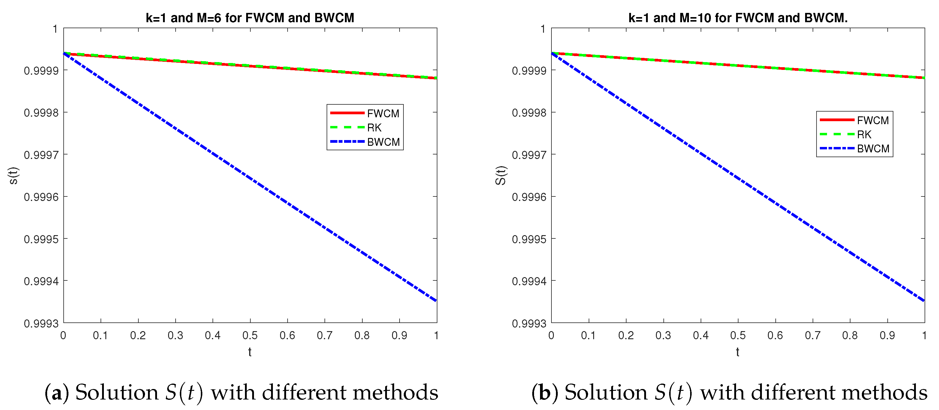
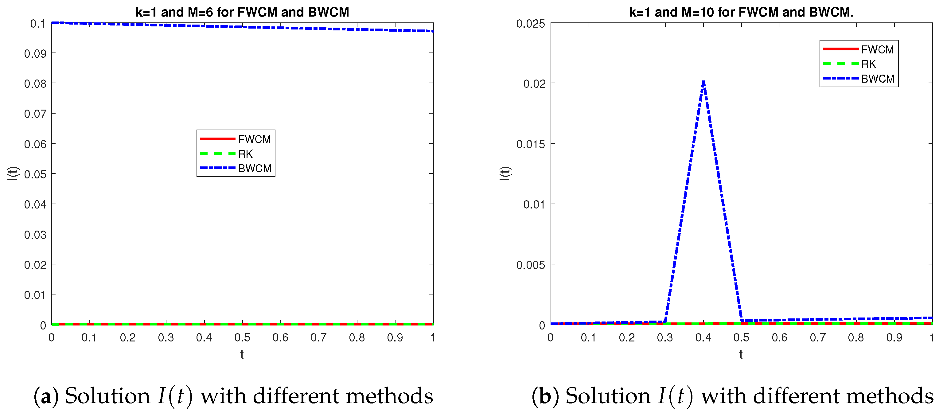
7. Comparison of Solutions Obtained from Different Numerical Methods (FWCM, BWCM, and RK4) and Their Error Analysis

On an 11th Gen Intel(R) Core(TM) i5-1135G7 @ 2.40GHz 1.38 GHz processor with 8 GB RAM, we used MATLAB R2023b for graphical representation and for numerical simulation.

We give our computational results here along with a discussion of them, taking into account the mathematical model given by Equations (33)–(35) and its initial conditions with the following specified parameters: $S\left(0\right)={\displaystyle \frac{\mathrm{5,070,822}}{\mathrm{5,071,126}}}$, $I\left(0\right)={\displaystyle \frac{304}{\mathrm{5,071,126}}}$, $R\left(0\right)=0.01$, $\alpha =0.006$, $\beta =0.333333$, $\gamma =0.375$, $\delta =0.02941$, and ${\mu }_h=0.0045$. After obtaining the solution from the FWCM, we examined it with the Runge–Kutta(RK4) and BWCM [13] solutions.

Table 1. Solution $S\left(t\right)$ obtained by RK, FWCM, and BWCM for $k=1$, $M=6$, and their error analysis.

t	FWCM For $\mathit{M}=6$	RK4	BWCM [13] for $\mathit{M}=6$	AE of FWCM with RK4 $1.0\times {10}^{-5}\times$	AE of BWCM with RK4 $1.0\times {10}^{-3}\times$
0	0.999938521568902	0.999940052761458	0.9999400527	0.153119255	0.000000061
0.1	0.999932605979405	0.999934089589839	0.9998801632	0.148361043	0.053926389
0.2	0.999926713883546	0.999928145307637	0.9998205524	0.143142409	0.107592907
0.3	0.999920844680790	0.999922219774398	0.9997610412	0.137509360	0.161178574
0.4	0.999914998190981	0.999916312853228	0.9997018124	0.131466224	0.214500453
0.5	0.999909174607655	0.999910424410677	0.9996427632	0.124980302	0.267661210
0.6	0.999903374451345	0.999904554316623	0.9995838457	0.117986527	0.320708616
0.7	0.999897598522890	0.999898702444166	0.9995252421	0.110392127	0.373460344
0.8	0.999891847856746	0.999892868669524	0.9994667214	0.102081277	0.426147269
0.9	0.999886123674291	0.999887052871929	0.9994084741	0.092919763	0.478578771
1.0	0.999880427337135	0.999881254933527	0.9993503412	0.082759639	0.530913733

,

Table 2. Solution $I\left(t\right)$ obtained by RK, FWCM, and BWCM for $k=1$, $M=6$, and their error analysis.

t	FWCM for $\mathit{M}=6$ $1.0\times {10}^{-3}\times$	RK4	BWCM [13] for $\mathit{M}=6$	AE of FWCM with RK4 $1.0\times {10}^{-4}\times$	AE of BWCM with RK4
0	0.151388595802287	0.599472385422882	0.1000000000	0.914413572	0.099940052
0.1	0.154675688981761	0.638746242903276	0.0997041574	0.908010646	0.099640282
0.2	0.157470598949661	0.676573124611832	0.0994216325	0.898132864	0.099353975
0.3	0.159736182347967	0.713001766004047	0.0991352365	0.884360057	0.099063936
0.4	0.161397910060683	0.748079270409903	0.0988563251	0.865899830	0.098781517
0.5	0.162338867907779	0.781851163670911	0.0985723652	0.841537515	0.098494180
0.6	0.162394757339147	0.814361446948217	0.0982942573	0.809586126	0.098212821
0.7	0.161348896128539	0.845652647763017	0.0980212547	0.767836313	0.097936689
0.8	0.158927219067519	0.875765872431373	0.0977476325	0.713506321	0.097660055
0.9	0.154793278659409	0.904740838229979	0.0974764251	0.643191948	0.097385951
1.0	0.148543245813239	0.932615950510128	0.0972080524	0.552816507	0.097114790

,

Table 3. Solution $R\left(t\right)$ obtained by RK, FWCM, and BWCM for $k=1$, $M=6$, and their error analysis.

t	FWCM for $\mathit{M}=6$	RK4	BWCM [13] for $\mathit{M}=6$	AE of FWCM with RK4 $1.0\times {10}^{-3}\times$	AE of BWCM with RK4
0	0.009463888096041	0.010000000000000	0.0000599472	0.536111903	0.009940052
0.1	0.009438569426823	0.009972928794027	0.0001169012	0.534359367	0.009856027
0.2	0.009415617923393	0.009946080047223	0.0001718139	0.530462123	0.009774266
0.3	0.009395362166263	0.009919447840034	0.0002247537	0.524085673	0.009694694
0.4	0.009378327425305	0.009893026447422	0.0201957869	0.514699022	0.010302760
0.5	0.009365295297659	0.009866810332378	0.0003249776	0.501515034	0.009541832
0.6	0.009357363345630	0.009840794139641	0.0003723877	0.483430794	0.009468406
0.7	0.009356004734595	0.009814972689638	0.0004180770	0.458967955	0.009396895
0.8	0.009363127870905	0.009789340972615	0.0004621033	0.426213101	0.009327237
0.9	0.009381136039787	0.009763894142974	0.0005045226	0.382758103	0.009259371
1.0	0.009412987043246	0.009738627513792	0.0005453889	0.325640470	0.009193238

,

Table 4. Solution $S\left(t\right)$ obtained by RK, FWCM, and BWCM for $k=1$, $M=10$, and their error analysis.

t	FWCM for $\mathit{M}=10$	RK4	BWCM [13] for $\mathit{M}=10$	AE of FWCM with RK4 $1.0\times {10}^{-13}\times$	AE of BWCM with RK4 $1.0\times {10}^{-3}\times$
0	0.999940052761381	0.999940052761458	0.9999400530	0.768274333	0.000000238
0.1	0.999934089589761	0.999934089589839	0.9998801861	0.778266340	0.053903489
0.2	0.999928145307559	0.999928145307637	0.9998205233	0.784927678	0.107622007
0.3	0.999922219774320	0.999922219774398	0.9997610628	0.782707232	0.161156974
0.4	0.999916312853151	0.999916312853228	0.9997018029	0.777156117	0.214509953
0.5	0.999910424410601	0.999910424410677	0.9996427419	0.757172102	0.267682510
0.6	0.999904554316550	0.999904554316623	0.9995838783	0.722755189	0.320676016
0.7	0.999898702444100	0.999898702444166	0.9995252103	0.657252030	0.373492144
0.8	0.999892868669469	0.999892868669524	0.9994667366	0.549560397	0.426132069
0.9	0.999887052871891	0.999887052871929	0.9994084556	0.373034936	0.478597271
1.0	0.999881254933518	0.999881254933527	0.9993503659	0.087707618	0.530889033

,

Table 5. Solution $I\left(t\right)$ obtained by RK, FWCM, and BWCM for $k=1$, $M=10$, and their error analysis.

t	FWCM for $\mathit{M}=10$ $1.0\times {10}^{-4}\times$	RK4 $1.0\times {10}^{-4}\times$	BWCM [13] for $\mathit{M}=10$	AE of FWCM with RK4 $1.0\times {10}^{-12}\times$	AE of BWCM with RK4
0	0.599472384428216	0.599472385422882	0.0000599472	0.099466652	0.000000000
0.1	0.638746242405969	0.638746242903276	0.0001169012	0.049730632	0.000053026
0.2	0.676573124582576	0.676573124611832	0.0001718139	0.002925611	0.000104156
0.3	0.713001766416621	0.713001766004047	0.0002247537	0.041257443	0.000153453
0.4	0.748079271242499	0.748079270409903	0.0201957869	0.083259544	0.020120978
0.5	0.781851164908085	0.781851163670911	0.0003249776	0.123717442	0.000246792
0.6	0.814361448583902	0.814361446948217	0.0003723877	0.163568431	0.000290951
0.7	0.845652649805132	0.845652647763017	0.0004180770	0.204211539	0.000333511
0.8	0.875765871805900	0.875765869328421	0.0004621033	0.247747907	0.000374526
0.9	0.904740841203290	0.904740838229979	0.0005045226	0.297331129	0.000414048
1.0	0.932615954086819	0.932615950510128	0.0005453889	0.357669108	0.000452127

and

Table 6. Solution $R\left(t\right)$ obtained by RK, FWCM, and BWCM for $k=1$, $M=10$, and their error analysis.

t	FWCM for $\mathit{M}=10$	RK4	BWCM [13] for $\mathit{M}=10$	AE of FWCM with RK4 $1.0\times {10}^{-12}\times$	AE of BWCM with RK4
0	0.009999999999813	0.010000000000000	0.1000000000	0.187115947	0.090000000
0.1	0.009972928793781	0.009972928794027	0.0997093188	0.245964706	0.089736390
0.2	0.009946080046923	0.009946080047223	0.0994213779	0.300114100	0.089475297
0.3	0.009919447839684	0.009919447840034	0.0991361027	0.349460044	0.089216654
0.4	0.009893026447029	0.009893026447422	0.0988534211	0.393600083	0.088960394
0.5	0.009866810331946	0.009866810332378	0.0985732633	0.431705018	0.088706452
0.6	0.009840794139179	0.009840794139641	0.0982955618	0.462303806	0.088454767
0.7	0.009814972689155	0.009814972689638	0.0980202512	0.482952219	0.088205278
0.8	0.009789340972125	0.009789340972615	0.0977472682	0.489708967	0.087957927
0.9	0.009763894142498	0.009763894142974	0.0974765517	0.476415781	0.087712657
1.0	0.009738627513358	0.009738627513792	0.0972080425	0.433632296	0.087469414

illustrate that the FWCM’s solutions are accurate and produce better approximations than the BWCM. In these tables, we have also compared Absolute Error (AE) of the proposed method and the BWCM with the RK4 method. As shown in Table 4, Table 5 and Table 6, Absolute Error (AE) decreases rapidly as we increase the value of M (maximal degree of the polynomial). We have also compared graphical solutions and Absolute Error (AE) obtained from the FWCM, BWCM, and RK4. Graphical representations of solutions obtained from the FWCM, BWCM, and RK4 are drawn in Figure 1, Figure 2 and Figure 3. From these figures, it is evident that the proposed method yields solutions that are significantly closer to the RK4 solution. A graphical comparison of Absolute Error obtained from the FWCM with RK4 and the BWCM with RK4 is shown in Figure 4, Figure 5 and Figure 6. The graph’s straight line indicates that the developed technique (FWCM) provides a better approximation than the BWCM method and produces a consistent absolute error at all places within the defined interval.

8. Conclusions

In this article, we have discussed a novel numerical approach called Fibonacci wavelet collocation method (FWCM) for the Dengue Fever model. Using Fibonacci wavelets, we constructed an operational matrix of integration that is used to estimate a dengue model. The efficiency and accuracy of the proposed method are demonstrated by comparing the obtained results with other existing methods, like Runge–Kutta (RK4) and BWCM [13]. The tables and figures clearly show that the FWCM outperforms the BWCM (when compared with RK4) and produces more consistent and accurate approximation results as M (maximal degree of the polynomial) increases. The error decreases more rapidly when we increase the degree (m) of the Fibonacci polynomials.

References

1. Guzman, M.G.; Harris, E. Dengue. Lancet 2015, 385, 453–465. [Google Scholar] [CrossRef] [PubMed]
2. Gould, E.; Pettersson, J.; Higgs, S.; Charrel, R.; De Lamballerie, X. Emerging arboviruses: Why today? One Health 2017, 4, 1–13. [Google Scholar] [CrossRef] [PubMed]
3. Bhatt, S.; Gething, P.W.; Brady, O.J.; Messina, J.P.; Farlow, A.W.; Moyes, C.L.; Drake, J.M.; Brownstein, J.S.; Hoen, A.G.; Sankoh, O.; et al. The global distribution and burden of dengue. Nature 2013, 496, 504–507. [Google Scholar] [CrossRef] [PubMed]
4. Buhler, C.; Winkler, V.; Runge-Ranzinger, S.; Boyce, R.; Horstick, O. Environmental methods for dengue vector control—A systematic review and meta-analysis. PLoS Negl. Trop. Dis. 2019, 13, e0007420. [Google Scholar] [CrossRef] [PubMed]
5. Simmons, C.P.; Farrar, J.J.; van Vinh Chau, N.; Wills, B. Dengue. N. Engl. J. Med. 2012, 366, 1423–1432. [Google Scholar] [CrossRef] [PubMed]
6. Nuraini, N.; Soewono, E.; Sidarto, K. Mathematical model of dengue disease transmission with severe dhf compartment. Bull. Malays. Math. Sci. Soc. 2007, 30, 143–157. [Google Scholar]
7. Yaacob, Y. Analysis of a dengue disease transmission model without immunity. Mat. Univ. Teknol. Malays. 2007, 23, 75–81. [Google Scholar]
8. Khalid, M.; Sultana, M.; Khan, F.S. Numerical Solution of SIR Model of Dengue Fever. Int. J. Comput. Appl. 2015, 118, 1–4. [Google Scholar] [CrossRef]
9. Rangkuti, Y.M.; Side, S.; Noorani, M.S.M. Numerical Analytic Solution of SIR Model of Dengue Fever Disease in South Sulawesi using Homotopy Perturbation Method and Variational Iteration Method. J. Math. Fundam. Sci. 2014, 46, 91–105. [Google Scholar] [CrossRef]
10. Mungkasi, S. Improved variational iteration solutions to the SIR model of dengue fever disease for the case of South Sulawesi. J. Math. Fundam. Sci. 2020, 52, 297–311. [Google Scholar] [CrossRef]
11. Umar, M.; Sabir, Z.; Raja, M.A.Z.; Sánchez, Y.G. A stochastic numerical computing heuristic of SIR nonlinear model based on dengue fever. Results Phys. 2020, 19, 103585. [Google Scholar] [CrossRef]
12. Lede, Y.K.; Mungkasi, S. Performance of the Runge-Kutta methods in solving a mathematical model for the spread of dengue fever disease. AIP Conf. Proc. 2019, 2202, 020044. [Google Scholar]
13. Li, F.; Baskonus, H.M.; Kumbinarasaiah, S.; Manohara, G.; Gao, W.; Ilhan, E. An Efficient Numerical Scheme for Biological Models in the Frame of Bernoulli Wavelets. Comput. Model. Eng. Sci. 2023, 137, 2381–2408. [Google Scholar] [CrossRef]
14. Bulut, F.; Oruç, Ö.; Esen, A. Higher order Haar wavelet method integrated with strang splitting for solving regularized long wave equation. Math. Comput. Simul. 2022, 197, 277–290. [Google Scholar] [CrossRef]
15. Keshavarz, E.; Ordokhani, Y.; Razzaghi, M. The Taylor wavelets method for solving the initial and boundary value problems of Bratu-type equations. Appl. Numer. Math. 2018, 128, 205–216. [Google Scholar] [CrossRef]
16. Rahimkhani, P.; Ordokhani, Y.; Babolian, E. Müntz-Legendre wavelet operational matrix of fractional-order integration and its applications for solving the fractional pantograph differential equations. Numer. Algorithms 2017, 77, 1283–1305. [Google Scholar] [CrossRef]
17. Sahu, P.K.; Ray, S.S. A new Bernoulli wavelet method for accurate solutions of nonlinear fuzzy Hammerstein–Volterra delay integral equations. Fuzzy Sets Syst. 2017, 309, 131–144. [Google Scholar] [CrossRef]
18. Yousefi, S.; Banifatemi, A. Numerical solution of Fredholm integral equations by using CAS wavelets. Appl. Math. Comput. 2006, 183, 458–463. [Google Scholar] [CrossRef]
19. Nemati, S.; Lima, P.M.; Torres, D.F.M. Numerical solution of a class of third-kind Volterra integral equations using Jacobi wavelets. Numer. Algorithms. 2021, 86, 675–691. [Google Scholar] [CrossRef]
20. Debnath, L.; Shah, F.A. Lecture Notes on Wavelet Transforms; Springer: Cham, Switzerland, 2017. [Google Scholar] [CrossRef]
21. Ahmad, K. Wavelet Packets and Their Statistical Applications; Springer: Singapore, 2018. [Google Scholar] [CrossRef]
22. Falcón, S.; Plaza, Á. On k–Fibonacci sequences and polynomials and their derivatives. Chaos Solitons Fractals 2009, 39, 1005–1019. [Google Scholar] [CrossRef]
23. Sabermahani, S.; Ordokhani, Y.; Yousefi, S. Fibonacci wavelets and their applications for solving two classes of time-varying delay problems. Optim. Control Appl. Methods. 2020, 41, 395–416. [Google Scholar] [CrossRef]
24. Irfan, M.; Shah, F.A.; Nisar, K.S. Fibonacci wavelet method for solving Pennes bioheat transfer equation. Int. J. Wavelets Multiresolut. Inf. Process. 2021, 19, 2150023. [Google Scholar] [CrossRef]
25. Rafiq, M.; Abdullah, A. Numerical Investigation using Fibonacci Wavelet Collocation Method for Solving Modified Unstable Nonlinear Schrödinger Equation. Int. J. Appl. Comput. Math 2023, 9, 118. [Google Scholar] [CrossRef]
Figure 1. Comparison of solution S ( t ) vs. t.
Mathematics 12 02565 g001
Figure 2. Comparison of solution I ( t ) vs. t.
Mathematics 12 02565 g002
Figure 3. Comparison of solution R ( t ) vs. t.
Mathematics 12 02565 g003
Figure 4. Comparison and error plots for S ( t ) vs. t.
Mathematics 12 02565 g004
Figure 5. Comparison and error plots for I ( t ) vs. t.
Mathematics 12 02565 g005
Figure 6. Comparison and error plots for R ( t ) vs. t.
Mathematics 12 02565 g006