Abstract
When aimed at minimizing both the classification error and the number of selected features, feature selection can be treated as a bi-objective optimization problem suitable for solving with multi-objective evolutionary algorithms (MOEAs). However, traditional MOEAs may encounter difficulties due to discrete optimization environments and the curse of dimensionality in the feature space, especially for high-dimensional datasets. Therefore, in this paper an interpolation-based evolutionary algorithm (termed IPEA) is proposed for tackling bi-objective feature selection in classification, where an interpolation based initialization method is designed for covering a wide range of search space and exploring the adaptively detected regions of interest. In experiments, IPEA is been compared with four state-of-the-art MOEAs in terms of two widely-used performance metrics on a list of 20 public real-world classification datasets with the dimensionality ranging from low to high. The overall empirical results suggest that IPEA generally performs the best of all tested algorithms, with significantly better search abilities and much lower computational time cost.
Keywords:
classification dataset; evolutionary algorithm; feature selection; multi-objective optimization MSC:
68W50
1. Introduction
As is known to all, evolutionary algorithms (EAs) have been widely used to solve optimization problems for decades [1], especially for multi-objective optimization problems (MOPs) with multiple contradictory objectives [2], which are then called the multi-objective evolutionary algorithms (MOEAs) [3]. Today, a great variety of MOEAs have been proposed from all around the world; these can be roughly divided into several categories: dominance-based [4,5,6], which adopt the nondominated sorting method for environmental selection; decomposition-based [7,8,9,10], which decompose an MOP into a series of simpler single-objective problems with weight vectors; indicator-based [11,12,13,14], which make use of a certain performance indicators for environmental selection; surrogate-based [15,16,17], which introduce a surrogate model for tackling expensive optimization problems; and multi-task [18,19,20], which generate multiple independent and cooperative tasks for different evolutionary purposes.
What is more, owing to their population-based search capability and ability to function without domain knowledge, MOEAs have also been applied for solving many real-world optimization problems [21,22,23], such as task offloading [24,25], network construction [26,27], community detection [28,29], and the feature selection problem [30,31] that is the focus of this work. To be more specific, feature selection is a common and important data preprocessing technique [32,33] which selects only a subset of useful features for classification rather than all of them. It is especially useful for large-scale datasets or those with high dimensionality [34]. When aimed at minimizing both the ratio of selected features and the ratio of classification errors, feature selection turns out to be a multi-objective (bi-objective) optimization problem, which can be formally described as follows [35]:
where M is the number of objectives, which in bi-objective feature selection is set to 2, D is the total number of features in the decision space, is the objective vector of , with denoting the objective value in the direction, is the decision vector of , where means selecting the ith feature and means not selecting that feature, and denotes the ratio of selected features, which can be further defined as follows:
with the discrete value ranging from 0 to 1 (i.e., ). Moreover, given the results in terms of (True Positive), (True Negative), (False Positive), and (False Negative), (representing the ratio of classification errors related to the above selected features) can be further defined as follows:
Despite of the aforementioned advantages, traditional MOEAs still face the curse of dimensionality in tackling bi-objective feature selection, which can cause the total number of features explodes. While many existing works have attempted to deal with this challenge [36,37], most of these have either introduced complicated frameworks or the need for many essential preset parameters. Moreover, it is difficult to balance the algorithm’s performance on both low-dimensional datasets and high-dimensional ones. Therefore, in this paper an interpolation-based EA (termed IPEA) is proposed that is specifically designed for tackling bi-objective feature selection in classification and is suitable for solving both low- and high-dimensional datasets. In IPEA, an interpolation-based initialization method is designed in order to provide a promising hybrid initial population that not only covers a wide range of search space but also allows the algorithm to explore adaptively within the most promising local areas of interest. In addition, a simple and efficient reproduction method is adopted to provide more population diversity and faster algorithm convergence during evolution. Combining the above-mentioned initialization and reproduction processes increases the search ability of IPEA in handling both low- and high-dimensional datasets.
The remainder of this paper is organized as follows: first, the related works are introduced in Section 2; then, the proposed IPEA is detailed in Section 3; the experimental setup is described in Section 4, while the empirical results are presented in Section 5; finally, the paper is concluded in Section 6.
2. Related Works
Evolutionary feature selection [38] can be generally categorized into wrapper-based and filter-based approaches [39,40]. In brief, the wrapper-based approaches [41,42] adopt a classification model such as SVM (Support Vector Machine) or KNN (K-Nearest Neighbors) [43] to evaluate the classification accuracy corresponding to the selected feature subset. By contrast, filter-based approaches [44,45] are independent of any classifier and directly analyze the classification data to explore the explicit or implicit relationships between features and the corresponding classes while ignoring the classification results of the feature subset, which is selected later. Therefore, wrapper-based approaches are relatively more accurate but typically have higher computational costs due to the additional classification process [20,46,47].
In this paper, a wrapper-based approach for evolutionary bi-objective feature selection is chosen. This is a widely used approach that has been discussed in many existing feature selection works over the last several years. For example, in 2020 Xu et al. [37] proposed a segmented initialization method and offspring modification method; however, the key parameter settings are all fixed and cannot be adaptively altered for different classification datasets or high-dimensional feature selection. Subsequently, Xu et al. [35] proposed an evolutionary algorithm named DAEA based on duplication analysis along with an efficient reproduction method; however, this algorithm’s performance has not been tested under the circumstances of high-dimensional feature selection. Following the idea of DAEA, Jiao et al. [48] further improved the method for handling solution duplication and designed a problem reformulation mechanism named PRDH; however, its applicability across different MOEA frameworks remains unconfirmed.
Therefore, this work attempts to design an interpolation based evolutionary algorithm, termed IPEA, which is suitable for tackling both relatively low-dimensional datasets and relatively high-dimensional ones. The framework of IPEA should be not as complicated as many other existing MOEAs designed for feature selection, and the algorithm should be able to effectively adapt to different optimization environment across a wide variety of features while maintaining a good balance between low- and high-dimensional datasets. This represents the major motivation behind this paper.
3. Proposed Algorithm
In this section, the general framework of the proposed algorithm IPEA is first introduced, then its two specially designed components, i.e., the initialization and reproduction processes, are illustrated further.
3.1. General Framework
The general framework of the IPEA is shown in Algorithm 1, where the population size N and number of total features D are input as the primary parameters. The general framework of IPEA is rather similar to traditional MOEAs, but uses the initialization and reproduction processes specially designed in this paper. Moreover, the environmental selection process has been modified by adding the ability to remove duplicated solutions in the current union population , as can be seen in Line 5 of Algorithm 1. Nevertheless, the widely-used truncation method based on nondominated sorting and crowding distances, first introduced in the classic dominance-based algorithm NSGA-II [4], is still adopted in IPEA to select and reserve the N best solutions in . The termination criterion of the IPEA is preset based on counting the number of evaluated objective functions, which is normally equal to the total number of generated solutions during evolution, as described in detail in Section 4.
| Algorithm 1 |
|
| Algorithm 2 |
|
3.2. Initialization Process
The initialization process of the IPEA is shown in Algorithm 2, which also invokes Algorithms 3–5. The initialization process is the major innovation of the IPEA, which is based on the utilization of interpolations in the objective space. Overall, the final initial population is made up of four hybrid subpopulations; while is based on a series of adaptively generated interpolation positions in the objective space, is based on the analysis of the previously generated . In turn, and are respectively inspired by the classic forward and backward search ideas in feature selection. To be more specific, the number of interpolation positions for new subpopulations generated in the objective space is adaptively set in Line 1 of Algorithm 2, the average interval between each two adjacent interpolation positions is accordingly set in Line 2 of Algorithm 2, and the standard interpolation subpopulation size is accordingly set in Line 3 of Algorithm 2. The detailed generation process of each interpolation-based subpopulation is shown from Line 5 to 15 in Algorithm 2, which is based on iteratively searching for the best objective value in all the subpopulations. During this process, Algorithm 3 is also invoked to generate new subpopulations according to the input interpolation position value. Another two pseudocodes, Algorithms 4 and 5, are respectively invoked to generate the forward search-inspired subpopulation and the backward search-inspired one. As can be seen in Algorithms 4 and 5, the former contains unique solutions with only one selected feature, while the later contains unique solutions with only one unselected feature.
| Algorithm 3 |
|
| Algorithm 4 |
|
| Algorithm 5 |
|
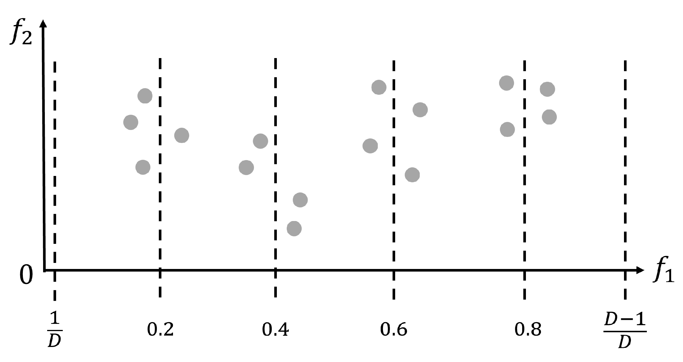
Figure 1 provides an illustrative example of how the adaptive interpolation-based initialization process in the IPEA works when the population size is set to . Thus, according to the previously introduced Algorithm 2, the number of interpolation positions is set to , the average interpolation interval is set to , and the standard size of each interpolation based subpopulation is set to . As can be seen from Figure 1, four interpolation-based subpopulations (together forming ) with an average size of four solutions are generated just around their related interpolation positions, i.e., 0.2, 0.4, 0.6, and 0.8. Apart from these four interpolation positions, two boundary interpolation positions, i.e., and , are also utilized, which respectively correspond to the previously introduced forward search-inspired subpopulation ( generated by Algorithm 4) and backward search-inspired subpopulation ( generated by Algorithm 5). In the case of Figure 1, the previously introduced best objective value lies in the subpopulation related to the 0.4 interpolation. Then, another new subpopulation with the full population size is generated by Algorithm 3 with the interpolation position value 0.4 input as the key parameter. In this way, a full population size of new solutions (i.e., ) is initialized around the most promising interpolation position found above. Therefore, combining all four of the above interpolation-related , as executed in Line 19 of Algorithm 2, covers a wide range of objective space while exploring adaptively within the boundary and promising local areas. It should be noted that in Figure 1 only shows with 16 solutions distributed, while the rest of , , and are not displayed in Figure 1.

Figure 1.
An example of how the adaptive interpolation-based initialization process in the IPEA works when the population size is set to .
3.3. Reproduction Process
The reproduction process of the IPEA is shown in Algorithm 6, which acts as an efficient supplement for the previously introduced interpolation-based initialization process. As can be seen from Algorithm 6, a totally random mating process first is conducted in Line 1 to select N pairs of parent solutions from the current population , indicating that every solution holds the same opportunity for reproduction. Then, the corresponding indexes with different decision variable values are found for each pair of parents; these are used in the later crossover operation. This is key to realizing efficient crossover, i.e., avoiding all invalid crossover operations between the same decision variable values. The adaptive crossover operation is shown from Line 4 to 9, which is based on the dynamic length of and a random integer limited by . After crossover, the mutation process is quite simple, adopting the traditional bitwise mutation method widely used in many other MOEAs. The bitwise mutation rate is set to , implying a relatively delicate and cautious mutation operation within a parent decision vector. Finally, the mutated parent solution is reserved as the expected new offspring.
| Algorithm 6 |
|
4. Experimental Setup
4.1. Comparison Algorithms
In this work, four state-of-the-art MOEAs are used as comparison algorithms against the proposed algorithm, IPEA. The compared algorithms are NSGA-II (a nondominated sorting based genetic algorithm) [4], MOEA/D (an MOEA based on decomposition) [7], MOEA/HD (an MOEA based on hierarchical decomposition) [10], and PMEA [13] (a polar metric-based evolutionary algorithm). To be more specific, NSGA-II and MOEA/D are among the most classic and well-known MOEAs, respectively based on dominance and decomposition; MOEA/HD is a recently published MOEA based on both dominance and decomposition, especially designed for solving MOPs with complex Pareto fronts; and PMEA is a recently published MOEA based on a performance indicator called the polar metric, which balances both the population diversity and the algorithm convergence during evolution. Overall, the three mainstream MOEA approaches, i.e., those based on dominance, decomposition and indicator, are all included in the experiments.
4.2. Classification Datasets
A total of 20 open-source classification datasets [49] are used as test problems to check the general optimization performances of all comparison algorithms for bi-objective feature selection. The attribute values of each tested dataset are shown in Table 1, with the total number of features sorted in ascending order. It can be seen from Table 1 that the total number of features for each dataset changes from 60 to 10,509, which covers a wide variety of features ranging from relatively lower to relatively higher dimensionality. Moreover, the number of classification samples changes from 50 to 606 and the number of corresponding classes changes from 2 to 15, suggesting the comprehensiveness of the test instances. In fact, most classification datasets used in this paper originate from real-world scenarios; for example, the “Sonar” dataset contains various patterns obtained by bouncing sonar signals off of a metal cylinder at various angles.

Table 1.
Attributes of each classification dataset used as test problems.
4.3. Performance Indicators
For comprehensive analyses based on empirical data, this paper uses multiple performance indicators to measure the general performance of all compared algorithms on all of the tested datasets. More specifically, the Hypervolume (HV) [50] indicator is used as the main metric to measure general optimization performance regarding both population diversity and algorithm convergence. The reference point for HV is uniformly set to in the bi-objective space. In addition, the Inverted Generation Distance Plus (IGD+) [51] indicator, which also covers the measurement of both diversity and convergence, is used to supplement the HV. The preference of IGD+ is highly related to the choice of reference points. Thus, for the sake of fairness, in this paper the reference points of IGD+ are set to the combination of all final nondominated solutions obtained by all of the tested algorithms. Normally, a greater HV value is preferable, while a smaller IGD+ value is preferable. Lastly, Wilcoxon’s test with a significance level is adopted to check the significant differences between each two compared algorithms; results below the level of significance are prefixed by the symbol ★.
4.4. Parameter Settings
In the experiments, all of the compared algorithms adopt the same parameter settings stated in the original papers. All algorithms are coded on an open-source MATLAB platform called PlatEMO [52]. Prior to evolution, each classification dataset is randomly divided into training and test subsets in a proportion of according to the stratified split process [35]. Then, a KNN () classification model is utilized with 10-fold cross-validation in order to avoid feature selection bias [53]. Lastly, each experimental run was independently executed 20 times, the population size for each algorithm was set to 100, and the termination criterion for each algorithm (i.e., the number of objective function evaluations) was set to 10,000, which is about 100 evolutionary generations.
5. Experimental Studies
In this section, the empirical results are first analyzed in terms of the HV and IGD+ metrics, shown in Table 2 and Table 3, respectively. In addition, the minimum classification error obtained by each algorithm along with the corresponding number of selected features are studied in Table 4. Then, the final nondominated solution distributions in the objective space, shown in Figure 2, are further analyzed. Finally, the computational time cost is analyzed by recording the experimental running time, with the results shown in Table 5.
Table 2.
Mean HV performance of each algorithm on each dataset, with the best results marked in gray (the greater the better) and insignificant differences prefixed by ★.
Table 3.
Mean IGD+ performance of each algorithm on each dataset, with the best results marked in gray (the smaller the better) and insignificant differences prefixed by ★.
Table 4.
Mean minimum classification errors obtained by each algorithm on each dataset, with the best results marked in gray (the smaller the better) and insignificant differences prefixed by ★. In addition, the mean rounded number of selected features (NSF) related to the obtained minimum classification error is shown beneath as NSF.
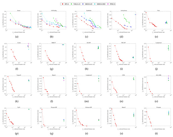
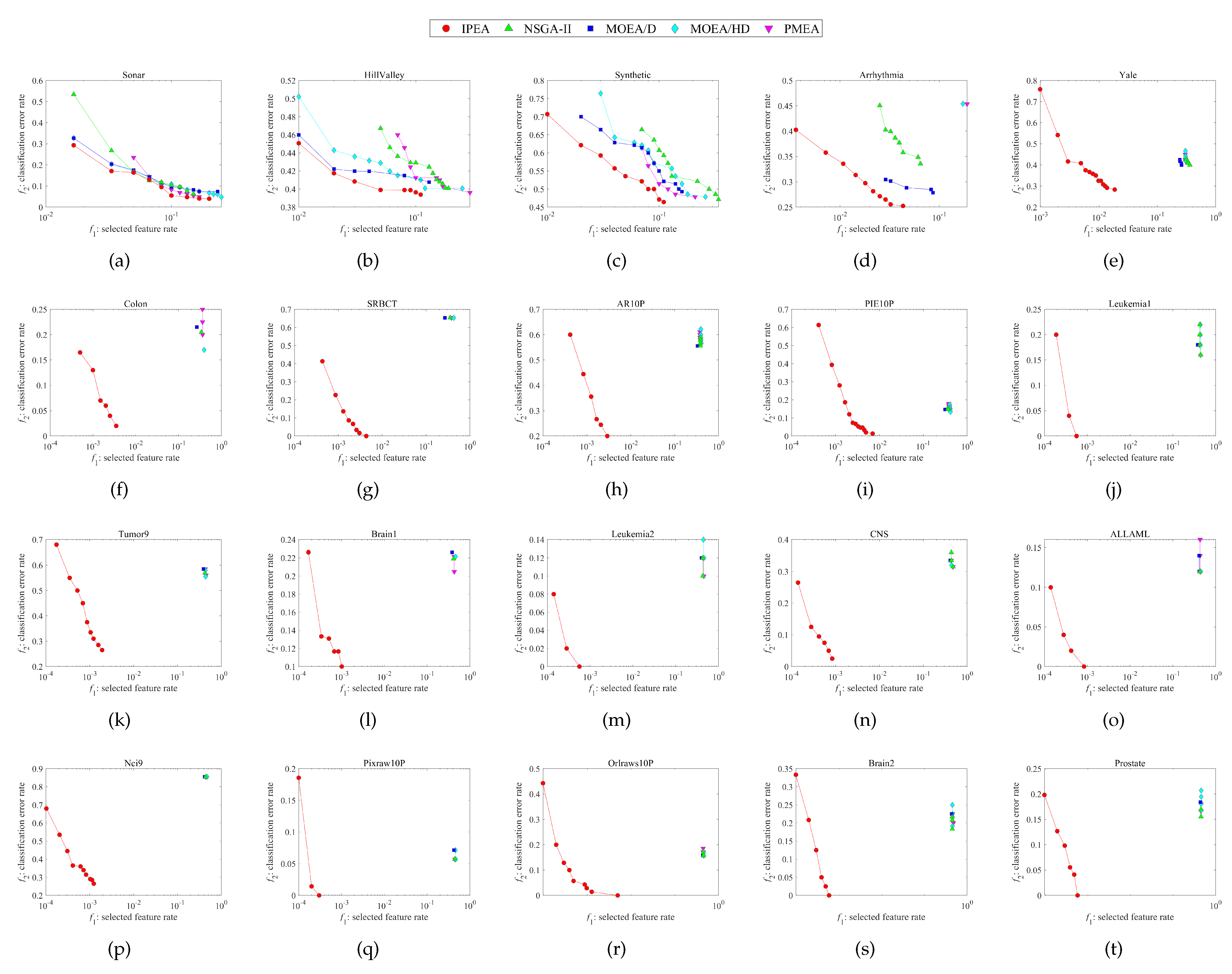
Figure 2.
Nondominated solution distributions in the objective space corresponding to the runs of median HV performances obtained by each algorithm on each dataset. (a) Sonar. (b) HillValley. (c) Synthetic. (d) Arrhythmia. (e) Yale. (f) Colon. (g) SRBCT. (h) AR10P. (i) PIE10P. (j) Leukemia1. (k) Tumor9. (l) Brain1. (m) Leukemia2. (n) CNS. (o) ALLAML. (p) Nci9. (q) Pixraw10P. (r) Orlraws10P. (s) Brain2. (t) Prostate.
Table 5.
Mean computational time cost in seconds for each algorithm run on each dataset, with the best results marked in gray (the smaller the better) and insignificant differences prefixed by ★.
5.1. Empirical Result Analyses
The general performance of each algorithm on all classification datasets in terms of the HV and IGD+ metrics is shown in Table 2 and Table 3, respectively, with the mean metric values and corresponding standard deviations displayed in each two rows. First, it can be seen from Table 2 and Table 3 that the proposed algorithm IPEA has the best performance of all the compared algorithms on all tested datasets, and the advantages of IPEA over all the other algorithms are rather significant on almost all of the tested datasets. Because both the HV and IGD+ metrics take the population diversity and convergence into consideration, the success of the IPEA in terms of these two metrics obviously suggests its superiority in both diversity and convergence. Moreover, the excellent performance of the IPEA on all of the datasets implies its great advantages and outstandingly effective search ability in tackling bi-objective feature selection not only for low-dimensional datasets but also for high-dimensional ones. In fact, the advantages of the IPEA in tackling the high-dimensional datasets appear to be even more obvious, showing huge differences in magnitude in the results shown in Table 3 due to the sparsity of feature space and the difficulty of finding more optimal solutions.
5.2. Classification Performance Analyses
The empirical results of each algorithm run on each dataset in terms of classification performance are shown in Table 4, with the mean minimum classification error values and corresponding mean number of selected features displayed in each two rows. First, it can be seen from Table 4 that the proposed IPEA has the best performance of all compared algorithms on all tested datasets in terms of the classification results. Again, the advantages of the IPEA over the other algorithms are quite significant on almost all the datasets, with the exception of the first two lower-dimensional ones, which do not fully challenge the IPEA’s search abilities. The minimum classification error (representing the best classification accuracy) obtained by the IPEA is generally much better than the other algorithms on each dataset. Moreover, because the corresponding number of selected features (shown as the NSF values in Table 4) generally affects the classification time and cost (as more selected features means more time and cost), the obviously superior NSF values obtained by the IPEA imply excellent computational efficiency, which actually proved in Section 5.4 below.
The implementation process of the whole wrapper-based evolutionary feature selection experiment is described as follows. At first, a population of N initial solutions containing different subsets of the selected features is evolved generation-by-generation. During this process, the selected features in each solution are only applied to training data that have been previously split from the tested datasets in a proportion of ; meanwhile a KNN () model and 10-fold cross-validation are executed for classification, returning the and objective values for the current solutions. When terminating the iterative evolution process, a set of nondominated solutions is selected from the last population, which is then applied to the test data to obtain the final classification results shown in Table 4 and the HV and IGD+ performance results shown in Table 2 and Table 3.
5.3. Nondominated Solution Distributions
The final nondominated solution distributions in the objective space obtained by each algorithm on each dataset are shown in Figure 2, along with 20 subfigures showing the final obtained nondominated solutions on the training data during evolution. For the sake of fairness, we choose the run with median HV performance from among 20 independent runs on each dataset. Because the nondominated solutions cannot be used to calculate the mean values, as there is no mean nondominated solution, we use the median performance here instead of the mean performance. Overall, it can be seen from Figure 2 that the IPEA obviously performs the best among all the algorithms, with more diverse solution distributions and more converged objective values in both the and directions.
To be more specific, the nondominated solution distributions of all the algorithms compared in the first four subfigures relate to relatively low-dimensional datasets. In Figure 2a–d the results appear quite similar, although the IPEA still performs the best. However, in the rest of the subfigures, i.e., Figure 2e–t, which are related to relatively high-dimensional datasets, the advantages of the IPEA in terms of the nondominated solution distributions become tremendous, leaving all the other algorithms’ nondominated solution distributions far behind.
Moreover, it can be observed from Figure 2 that the nondominated solution distributions are relatively sparse on the high-dimensional datasets compared to the low-dimensional datasets. This is because the feature space or search space becomes sparser as the number of total features increases, making it much more difficult for MOEAs to find enough optimal solutions during evolution. This phenomenon also happens to the proposed IPEA; however, the negative impact is been greatly reduced compared with the other algorithms.
5.4. Computational Time Analyses
The mean computational time cost for each algorithm run on each dataset is recorded in seconds, with the results shown in Table 5. It can be seen from Table 5 that the mean computational time cost of the IPEA is always the smallest among all the algorithms on each dataset, with significant advantages over all other algorithms. Moreover, the advantages of the IPEA in terms of the computational time are even more significant on the relatively high-dimensional datasets, generally incurring only half the other algorithms’ mean computational time cost. In fact, if only considering the MOEA framework, the theoretical time complexity of IPEA is not very different from that of many other traditional MOEAs, as the general framework of the IPEA inherits the basic ideas of most MOEAs. The worst theoretical time complexity of the IPEA can be estimated as with M as the number of objectives and N as the population size, which mainly comes from the process of nondominated sorting. However, the real running time of the IPEA on each dataset is much smaller than the theoretical expectations. This is mainly because the IPEA saves a great deal of time during the classification process owing to its better selection of feature subsets, with much smaller numbers of selected features being used for classification. Therefore, the computational efficiency of the IPEA regarding the whole evolutionary feature selection process is rather time-saving, with significant efficiency advantages over the compared algorithms on each tested dataset, including both the relatively low-dimension and relatively high-dimension ones.
6. Conclusions
In this work, an interpolation-based EA (termed the IPEA) is proposed for tackling bi-objective feature selection on both low-dimensional and high-dimensional classification datasets. The design of the IPEA incorporates an interpolation-based initialization method in order to provide a promising hybrid initial population, allowing it to cover a wide range of search space while adaptively exploring the regions of interest. Moreover, an efficient reproduction method is adopted to provide greater population diversity and better algorithm convergence during evolution. The framework of the IPEA is simple but effective, and can adapt to different kinds of optimization environments across a wide variety of features. The outstanding performance and significant advantages of the IPEA have been verified in the experiments and comprehensively analyzed. When compared with four state-of-the-art MOEAs on a list of 20 public real-world classification datasets, the IPEA always performs best in terms of two widely-used performance metrics, showing excellent search abilities. Furthermore, the IPEA also shows the best performance in terms of the final nondominated solution distributions in the objective space, and is proven to be the most computationally efficient among all tested algorithms in terms of the real running time recorded on each tested dataset.
In future work, it is planned to study the feasibility of the proposed algorithm IPEA on additional kinds of discrete optimization problems, such as neural network construction and community node detection.
Funding
This research was funded by National Natural Science Foundation of China (grant number 62103209), the Natural Science Foundation of Fujian Province (grant number 2020J05213), the Scientific Research Project of Putian Science and Technology Bureau (grant number 2021ZP07), the Startup Fund for Advanced Talents of Putian University (grant number 2019002), and the Research Projects of Putian University (grant number JG202306).
Data Availability Statement
The data presented in this study are available on request from the corresponding author.
Acknowledgments
This work was supported in part by the National Natural Science Foundation of China under Grant 62103209, by the Natural Science Foundation of Fujian Province under Grant 2020J05213, by the Scientific Research Project of Putian Science and Technology Bureau under Grant 2021ZP07, by the Startup Fund for Advanced Talents of Putian University under Grant 2019002, and by the Research Projects of Putian University under Grant JG202306.
Conflicts of Interest
The author declares no conflicts of interest.
References
- Eiben, A.E.; Smith, J.E. What is an evolutionary algorithm? In Introduction to Evolutionary Computing; Springer: Berlin/Heidelberg, Germany, 2015; pp. 25–48. [Google Scholar]
- Coello, C.A.C.; Lamont, G.B.; Van Veldhuizen, D.A. Evolutionary Algorithms for Solving Multi-Objective Problems; Springer: New York, NY, USA, 2007; Volume 5. [Google Scholar]
- Zhou, A.; Qu, B.Y.; Li, H.; Zhao, S.Z.; Suganthan, P.N.; Zhang, Q. Multiobjective evolutionary algorithms: A survey of the state of the art. Swarm Evol. Comput. 2011, 1, 32–49. [Google Scholar]
- Deb, K.; Pratap, A.; Agarwal, S.; Meyarivan, T. A fast and elitist multiobjective genetic algorithm: NSGA-II. IEEE Trans. Evol. Comput. 2002, 6, 182–197. [Google Scholar] [CrossRef]
- Deb, K.; Jain, H. An Evolutionary Many-Objective Optimization Algorithm Using Reference-Point-Based Nondominated Sorting Approach, Part I: Solving Problems With Box Constraints. IEEE Trans. Evol. Comput. 2014, 18, 577–601. [Google Scholar] [CrossRef]
- Tian, Y.; Cheng, R.; Zhang, X.; Su, Y.; Jin, Y. A Strengthened Dominance Relation Considering Convergence and Diversity for Evolutionary Many-Objective Optimization. IEEE Trans. Evol. Comput. 2019, 23, 331–345. [Google Scholar]
- Zhang, Q.; Li, H. MOEA/D: A Multiobjective Evolutionary Algorithm Based on Decomposition. IEEE Trans. Evol. Comput. 2007, 11, 712–731. [Google Scholar] [CrossRef]
- Li, H.; Zhang, Q. Multiobjective Optimization Problems With Complicated Pareto Sets, MOEA/D and NSGA-II. IEEE Trans. Evol. Comput. 2009, 13, 284–302. [Google Scholar] [CrossRef]
- Li, K.; Zhang, Q.; Kwong, S.; Li, M.; Wang, R. Stable Matching-Based Selection in Evolutionary Multiobjective Optimization. IEEE Trans. Evol. Comput. 2014, 18, 909–923. [Google Scholar] [CrossRef]
- Xu, H.; Zeng, W.; Zhang, D.; Zeng, X. MOEA/HD: A Multiobjective Evolutionary Algorithm Based on Hierarchical Decomposition. IEEE Trans. Cybern. 2019, 49, 517–526. [Google Scholar] [CrossRef]
- Bader, J.; Zitzler, E. HypE: An Algorithm for Fast Hypervolume-Based Many-Objective Optimization. Evol. Comput. 2011, 19, 45–76. [Google Scholar] [CrossRef]
- Liang, Z.; Luo, T.; Hu, K.; Ma, X.; Zhu, Z. An Indicator-Based Many-Objective Evolutionary Algorithm With Boundary Protection. IEEE Trans. Cybern. 2021, 51, 4553–4566. [Google Scholar] [CrossRef]
- Xu, H.; Zeng, W.; Zeng, X.; Yen, G.G. A Polar-Metric-Based Evolutionary Algorithm. IEEE Trans. Cybern. 2021, 51, 3429–3440. [Google Scholar] [CrossRef] [PubMed]
- Lopes, C.L.d.V.; Martins, F.V.C.; Wanner, E.F.; Deb, K. Analyzing Dominance Move (MIP-DoM) Indicator for Multiobjective and Many-Objective Optimization. IEEE Trans. Evol. Comput. 2022, 26, 476–489. [Google Scholar] [CrossRef]
- Wang, H.; Jin, Y.; Sun, C.; Doherty, J. Offline data-driven evolutionary optimization using selective surrogate ensembles. IEEE Trans. Evol. Comput. 2018, 23, 203–216. [Google Scholar]
- Lin, Q.; Wu, X.; Ma, L.; Li, J.; Gong, M.; Coello, C.A.C. An Ensemble Surrogate-Based Framework for Expensive Multiobjective Evolutionary Optimization. IEEE Trans. Evol. Comput. 2022, 26, 631–645. [Google Scholar] [CrossRef]
- Sonoda, T.; Nakata, M. Multiple Classifiers-Assisted Evolutionary Algorithm Based on Decomposition for High-Dimensional Multiobjective Problems. IEEE Trans. Evol. Comput. 2022, 26, 1581–1595. [Google Scholar] [CrossRef]
- Da, B.; Gupta, A.; Ong, Y.S.; Feng, L. Evolutionary multitasking across single and multi-objective formulations for improved problem solving. In Proceedings of the 2016 IEEE Congress on Evolutionary Computation (CEC), Vancouver, BC, Canada, 24–29 July 2016; IEEE: Piscataway, NJ, USA, 2016; pp. 1695–1701. [Google Scholar]
- Gupta, A.; Ong, Y.S.; Feng, L.; Tan, K.C. Multiobjective Multifactorial Optimization in Evolutionary Multitasking. IEEE Trans. Cybern. 2017, 47, 1652–1665. [Google Scholar]
- Chen, K.; Xue, B.; Zhang, M.; Zhou, F. Evolutionary Multitasking for Feature Selection in High-Dimensional Classification via Particle Swarm Optimization. IEEE Trans. Evol. Comput. 2022, 26, 446–460. [Google Scholar] [CrossRef]
- Cao, F.; Tang, Z.; Zhu, C.; Zhao, X. An Efficient Hybrid Multi-Objective Optimization Method Coupling Global Evolutionary and Local Gradient Searches for Solving Aerodynamic Optimization Problems. Mathematics 2023, 11, 3844. [Google Scholar] [CrossRef]
- Garces-Jimenez, A.; Gomez-Pulido, J.M.; Gallego-Salvador, N.; Garcia-Tejedor, A.J. Genetic and Swarm Algorithms for Optimizing the Control of Building HVAC Systems Using Real Data: A Comparative Study. Mathematics 2021, 9, 2181. [Google Scholar] [CrossRef]
- Ramos-Pérez, J.M.; Miranda, G.; Segredo, E.; León, C.; Rodríguez-León, C. Application of Multi-Objective Evolutionary Algorithms for Planning Healthy and Balanced School Lunches. Mathematics 2021, 9, 80. [Google Scholar] [CrossRef]
- Long, S.; Zhang, Y.; Deng, Q.; Pei, T.; Ouyang, J.; Xia, Z. An Efficient Task Offloading Approach Based on Multi-Objective Evolutionary Algorithm in Cloud-Edge Collaborative Environment. IEEE Trans. Netw. Sci. Eng. 2023, 10, 645–657. [Google Scholar] [CrossRef]
- Zhang, Z.; Ma, S.; Jiang, X. Research on Multi-Objective Multi-Robot Task Allocation by Lin-Kernighan-Helsgaun Guided Evolutionary Algorithms. Mathematics 2022, 10, 4714. [Google Scholar] [CrossRef]
- Xue, Y.; Chen, C.; Slowik, A. Neural Architecture Search Based on a Multi-Objective Evolutionary Algorithm With Probability Stack. IEEE Trans. Evol. Comput. 2023, 27, 778–786. [Google Scholar] [CrossRef]
- Ponti, A.; Candelieri, A.; Giordani, I.; Archetti, F. Intrusion Detection in Networks by Wasserstein Enabled Many-Objective Evolutionary Algorithms. Mathematics 2023, 11, 2342. [Google Scholar] [CrossRef]
- Zhu, W.; Li, H.; Wei, W. A Two-Stage Multi-Objective Evolutionary Algorithm for Community Detection in Complex Networks. Mathematics 2023, 11, 2702. [Google Scholar] [CrossRef]
- Gao, C.; Yin, Z.; Wang, Z.; Li, X.; Li, X. Multilayer Network Community Detection: A Novel Multi-Objective Evolutionary Algorithm Based on Consensus Prior Information [Feature]. IEEE Comput. Intell. Mag. 2023, 18, 46–59. [Google Scholar] [CrossRef]
- Xu, H.; Xue, B.; Zhang, M. A Bi-Search Evolutionary Algorithm for High-Dimensional Bi-Objective Feature Selection. IEEE Trans. Emerg. Top. Comput. Intell. 2024, 1–14. [Google Scholar] [CrossRef]
- Xu, H.; Xue, B.; Zhang, M. Probe Population Based Initialization and Genetic Pool Based Reproduction for Evolutionary Bi-Objective Feature Selection. IEEE Trans. Evol. Comput. 2024, 1. [Google Scholar] [CrossRef]
- Nguyen, B.H.; Xue, B.; Andreae, P.; Ishibuchi, H.; Zhang, M. Multiple Reference Points-Based Decomposition for Multiobjective Feature Selection in Classification: Static and Dynamic Mechanisms. IEEE Trans. Evol. Comput. 2020, 24, 170–184. [Google Scholar] [CrossRef]
- Khalid, S.; Khalil, T.; Nasreen, S. A survey of feature selection and feature extraction techniques in machine learning. In Proceedings of the 2014 Science and Information Conference, London, UK, 27–29 August 2014; pp. 372–378. [Google Scholar] [CrossRef]
- Cheng, F.; Cui, J.; Wang, Q.; Zhang, L. A Variable Granularity Search-Based Multiobjective Feature Selection Algorithm for High-Dimensional Data Classification. IEEE Trans. Evol. Comput. 2023, 27, 266–280. [Google Scholar] [CrossRef]
- Xu, H.; Xue, B.; Zhang, M. A Duplication Analysis-Based Evolutionary Algorithm for Biobjective Feature Selection. IEEE Trans. Evol. Comput. 2021, 25, 205–218. [Google Scholar] [CrossRef]
- Cheng, F.; Chu, F.; Xu, Y.; Zhang, L. A Steering-Matrix-Based Multiobjective Evolutionary Algorithm for High-Dimensional Feature Selection. IEEE Trans. Cybern. 2022, 52, 9695–9708. [Google Scholar] [CrossRef] [PubMed]
- Xu, H.; Xue, B.; Zhang, M. Segmented Initialization and Offspring Modification in Evolutionary Algorithms for Bi-Objective Feature Selection. In Proceedings of the 2020 Genetic and Evolutionary Computation Conference, GECCO’20, Cancun, Mexico, 8–12 July 2020; pp. 444–452. [Google Scholar]
- De La Iglesia, B. Evolutionary computation for feature selection in classification problems. Wiley Interdiscip. Rev. Data Min. Knowl. Discov. 2013, 3, 381–407. [Google Scholar]
- Xue, B.; Zhang, M.; Browne, W.N.; Yao, X. A survey on evolutionary computation approaches to feature selection. IEEE Trans. Evol. Comput. 2015, 20, 606–626. [Google Scholar]
- Dokeroglu, T.; Deniz, A.; Kiziloz, H.E. A comprehensive survey on recent metaheuristics for feature selection. Neurocomputing 2022, 494, 269–296. [Google Scholar]
- Mukhopadhyay, A.; Maulik, U. An SVM-wrapped multiobjective evolutionary feature selection approach for identifying cancer-microRNA markers. IEEE Trans. Nanobiosci. 2013, 12, 275–281. [Google Scholar]
- Vignolo, L.D.; Milone, D.H.; Scharcanski, J. Feature selection for face recognition based on multi-objective evolutionary wrappers. Expert Syst. Appl. 2013, 40, 5077–5084. [Google Scholar]
- Guyon, I.; Elisseeff, A. An introduction to variable and feature selection. J. Mach. Learn. Res. 2003, 3, 1157–1182. [Google Scholar]
- Lazar, C.; Taminau, J.; Meganck, S.; Steenhoff, D.; Coletta, A.; Molter, C.; de Schaetzen, V.; Duque, R.; Bersini, H.; Nowe, A. A survey on filter techniques for feature selection in gene expression microarray analysis. IEEE/ACM Trans. Comput. Biol. Bioinform. TCBB 2012, 9, 1106–1119. [Google Scholar]
- Xue, B.; Cervante, L.; Shang, L.; Browne, W.N.; Zhang, M. Multi-objective evolutionary algorithms for filter based feature selection in classification. Int. J. Artif. Intell. Tools 2013, 22, 1350024. [Google Scholar]
- Xue, B.; Zhang, M.; Browne, W.N. Particle swarm optimisation for feature selection in classification: Novel initialisation and updating mechanisms. Appl. Soft Comput. 2014, 18, 261–276. [Google Scholar]
- Chen, K.; Xue, B.; Zhang, M.; Zhou, F. An Evolutionary Multitasking-Based Feature Selection Method for High-Dimensional Classification. IEEE Trans. Cybern. 2022, 52, 7172–7186. [Google Scholar] [CrossRef] [PubMed]
- Jiao, R.; Xue, B.; Zhang, M. Solving Multi-objective Feature Selection Problems in Classification via Problem Reformulation and Duplication Handling. IEEE Trans. Evol. Comput. 2022, 28, 846–860. [Google Scholar] [CrossRef]
- Kelly, M.; Longjohn, R.; Nottingham, K. The UCI Machine Learning Repository. Available online: https://archive.ics.uci.edu (accessed on 18 August 2024).
- While, L.; Hingston, P.; Barone, L.; Huband, S. A faster algorithm for calculating Hypervolume. IEEE Trans. Evol. Comput. 2006, 10, 29–38. [Google Scholar]
- Ishibuchi, H.; Imada, R.; Masuyama, N.; Nojima, Y. Comparison of Hypervolume, IGD and IGD+ from the Viewpoint of Optimal Distributions of Solutions. In Proceedings of the Evolutionary Multi-Criterion Optimization 2019, East Lansing, MI, USA, 10–13 March 2019; Deb, K., Goodman, E., Coello Coello, C.A., Klamroth, K., Miettinen, K., Mostaghim, S., Reed, P., Eds.; Springer: Cham, Switzerland, 2019; pp. 332–345. [Google Scholar]
- Tian, Y.; Cheng, R.; Zhang, X.; Jin, Y. PlatEMO: A MATLAB Platform for Evolutionary Multi-Objective Optimization. IEEE Comput. Intell. Mag. 2017, 12, 73–87. [Google Scholar]
- Tran, B.; Xue, B.; Zhang, M.; Nguyen, S. Investigation on particle swarm optimisation for feature selection on high-dimensional data: Local search and selection bias. Connect. Sci. 2016, 28, 270–294. [Google Scholar]
Disclaimer/Publisher’s Note: The statements, opinions and data contained in all publications are solely those of the individual author(s) and contributor(s) and not of MDPI and/or the editor(s). MDPI and/or the editor(s) disclaim responsibility for any injury to people or property resulting from any ideas, methods, instructions or products referred to in the content. |
© 2024 by the author. Licensee MDPI, Basel, Switzerland. This article is an open access article distributed under the terms and conditions of the Creative Commons Attribution (CC BY) license (https://creativecommons.org/licenses/by/4.0/).