Polynomial Iterative Learning Control (ILC) Tracking Control Design for Uncertain Repetitive Continuous-Time Linear Systems Applied to an Active Suspension of a Car Seat ^†

Abstract

This paper addresses the issue of polynomial iterative learning tracking control (Poly-ILC) for continuous-time linear systems (LTI) operating repetitively. It explores the design of an iterative learning control law by examining the stability along the pass theory of 2D repetitive systems. The obtained result is a generalization of the notion of stability along passages, taking into account transient performances. To strike a balance between stability along passages and transient performance, we extend our developed result in the discrete case, relying on some numerical tools. Specifically, in this work we investigate the convergence of tracking error with given learning controller gains. The key contribution of this structure of control lies in establishing an LMI (linear matrix inequality) condition that ensures both pole placement according to desired specifications and the convergence of output error between iterations. Furthermore, new sufficient conditions for stability regions along the pass addressing the tracking problem of differential linear repetitive processes are developed. Numerical results are provided to demonstrate the effectiveness of the proposed approaches.

1. Introduction

Iterative learning control (ILC) emerges as a potent tool for mitigating tracking errors in systems that operate repetitively. It has been heralded as a control strategy capable of enhancing the performance of systems engaged in batch repetitive servo tasks [1,2,3]. Over the past two decades, ILC has consistently drawn attention. The treatment of tracking problems within the ILC framework often necessitates consideration of certain 2D properties. Utilizing the delay operator in the time domain (via standard Laplace transformation), ref. [2] translates the dynamics of linear continuous-time systems into an iterative process, applicable to time-invariant parameters, input variables, output variables, and errors. This extension allows for the exploration of tracking and stabilization problems, a topic not extensively addressed in the literature despite its intrinsic connection to fundamental control issues like stability and stabilization. These core control problems can be readily extended to encompass robustness analysis and additional control performance specifications using norms [4,5,6,7]. Consequently, within the realm of robust analysis and control synthesis for uncertain linear systems, many results can be characterized by LMIs [2,8,9,10]. In the case of the studied LRP systems, the stability analysis of the system boils down to verifying the convergence of the tracking error to zero. Asymptotic stability of a repetitive system implies that the system’s response approaches a stable behavior over time. Specifically, it means that as time goes to infinity, the system’s output settles into a steady-state behavior where it remains bounded and does not exhibit any oscillatory behavior. Consequently, if a repetitive system is asymptotically stable, it suggests that any error between the desired output (reference signal) and the actual output of the system will tend to decrease and eventually converge to zero as time progresses [11,12]. This is because the system’s dynamics, under asymptotic stability, ensure that any deviations from the desired behavior diminish over time until the system reaches a state of equilibrium where the error becomes negligible. In summary, the convergence of the tracking error to zero is a consequence of the asymptotic stability of a repetitive system, indicating that the system’s response settles into a stable behavior over time, with the error between the desired and actual outputs approaching zero. In this context, the ILC tracking problem has been reformulated into a stability analysis concept along the pass of 2D repetitive systems [11,12]. A necessary and sufficient condition ensuring stability along the pass has been devised. This new formulation offers insight into the problem within the realm of 2D repetitive systems [13]. The primary contribution of this paper lies in providing the LMI characterization for stability along the pass and subsequently addressing the tracking error problem of continuous-time linear systems operating repetitively. Specifically, the theory of stability along the pass, employing the LMI condition to the processes, yields three conditions [14,15,16,17], as discussed earlier, which can be verified through direct application of the LMI condition. Two of these tests necessitate that the eigenvalues of the matrices describing the previous pass profile contribution to the current pass profile and the current pass state vector contribution to the along the pass dynamics lie within the open unit circle and the open left half of the complex plane, respectively [18]. Furthermore, this paper aims to provide a rigorous LMI characterization for stability along the pass to synthesize an ILC law guaranteeing asymptotic stability of the closed-loop repetitive system for any current pass state vector while ensuring three different performances simultaneously [19]. These performances include asymptotic stability with specified transient response and damping factor [20,21,22] determined by the pole locations of repetitive closed-loop linear systems. Polynomial iterative learning tracking (P-ILC) control is a method used to improve the tracking performance of repetitive systems over multiple iterations. It relies on the concept of learning from past errors to iteratively adjust the control input, aiming to reduce the tracking error between the desired and actual outputs. At its core, P-ILC is based on the notion of iterative learning, where the control input is updated at each iteration based on the error observed in the previous iterations. This iterative process allows the controller to gradually learn the system dynamics and improve its performance over time. The theoretical foundations of P-ILC involve several key concepts. First is the use of polynomial functions to model the desired trajectory of the system’s output. These polynomial trajectories provide a flexible and adaptable framework for defining the desired behavior of the system over time [19,23]. Second is the incorporation of a learning mechanism that adjusts the control input based on the error between the actual and desired outputs. This learning mechanism typically involves updating the control input using a combination of past error measurements and a learning rate parameter, which governs the rate at which the controller adapts to changes in the system. In the context of repetitive continuous-time linear systems, P-ILC offers several advantages. By leveraging the repetitive nature of the system, P-ILC can exploit the similarities between successive iterations to improve tracking performance more efficiently. Additionally, the use of polynomial trajectories allows for smoother and more continuous tracking, which can be particularly beneficial for systems with continuous dynamics. Overall, the theoretical foundations of P-ILC provide a robust framework for improving the tracking performance of repetitive continuous-time linear systems. By combining the principles of iterative learning with polynomial trajectory modeling, P-ILC offers a flexible and effective approach to achieving accurate and reliable tracking in various applications [18]. The proposed idea in this work is, roughly, to evolve a nominal control law towards a more robust control law, thus elaborating the concept of stability along the iteration of LRP systems in this sense. This approach can be called D-stability along the iteration. Specifically, and in coherence with the objectives, it involves pole placement while satisfying the notion of stability along the iteration that is presented. Indeed, concerning the set objectives and satisfied requirements, they fall into two categories. On the one hand, there is stability and stabilization of LRP systems along the iteration while ensuring desired transient performance. On the other hand, there is the concept of D-stability along the iteration, which will be reformulated later as a tracking problem.Given the significance of ILC, this paper furnishes results necessary both for solving tracking problems and for ensuring diverse performances for proportional-type ILC and polynomial-type ILC. It demonstrates that robust stability and controller synthesis for continuous linear repetitive processes become feasible through efficient numerical techniques based on LMIs. Building upon these modeling and control methods, this paper establishes a polynomial-type ILC law and proposes a sufficient condition to achieve high-speed tracking control [24,25]. The remainder of this paper is structured as follows: Section 2 presents the problem formulation, introducing the concept of stability along the pass and providing LMI conditions to ensure this stability. In Section 3, the focus shifts to harnessing the ILC tracking problem, where the convergence of tracking error to zero and pole placement performance depend on the selection of suitable learning controller gains. The convergence condition for the tracking error problem is derived using 2D system theory and LMI formulation. Section 4 reveals that convergence and learning performance of this ILC scheme can be achieved through polynomial ILC controller design. Finally, numerical simulations are provided to demonstrate the efficacy of the proposed method.

Throughout this paper, for the designs and simulations, the software MATLAB 2019b was used. The null matrix and the identity matrix with appropriate dimensions are denoted by 0 and I, respectively. Moreover, the notation $X\ge Y$ (respectively, $X>Y$) means that the matrix $X-Y$ is positive semi-definite (respectively, positive definite). In large matrix expressions, the symbol ∗ replaces terms that are induced by symmetry. The expression $\rho \left(\right)$ denotes the spectral radius of its matrix argument. Finally, the $∥ ∥$ denotes the induced operator norm, and the Laplace transform is an s-transform.

2. Problem Statement and Preliminaries

Stability along the Pass for 2D Repetitive Systems

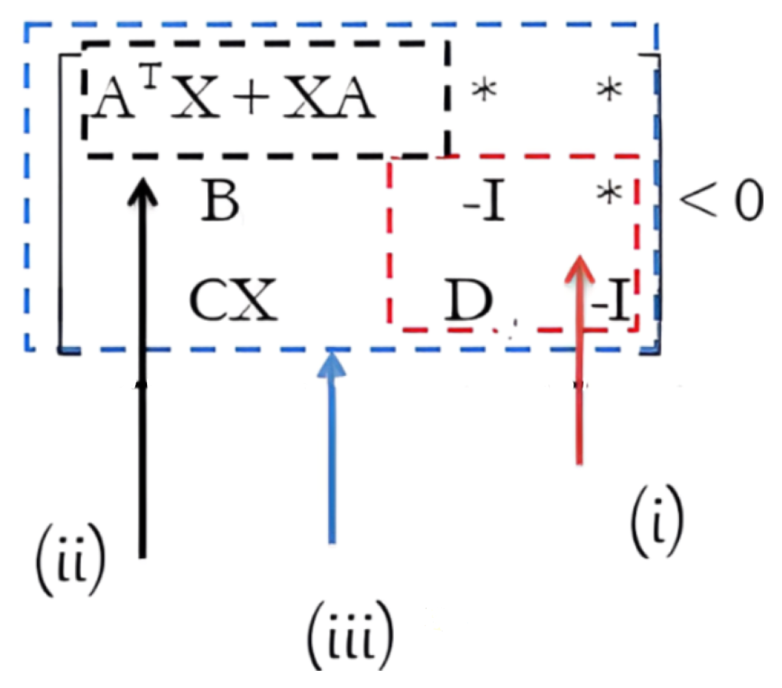
The state-space model of a continuous linear repetitive process has the following form over $t\in \left[0,T\right]$ and $k\in I{R}_{+}$:

$$\left\{\begin{array}{c}{\dot{x}}_k\left(t\right)=A{x}_k\left(t\right)+B{u}_k\left(t\right)\\ y_k\left(t\right)=C{x}_k\left(t\right)+D{u}_k\left(t\right)\end{array}\right.x\left(0\right)=0,t\ge 0,k>0$$

(1)

where A, B, and C are a constant matrix; $x_{k+1}\left(t\right)\in I{R}^n$ is the state vector; $u_{k+1}\left(t\right)\in I{R}^m$ and $y_{k+1}\left(t\right)\in I{R}^p$ are the input and the output of the system, successively; and $x_0$ is the initial condition for each iteration. The stability challenge in linear repetitive processes arises from the potential presence of oscillations within the sequence of pass profiles, with oscillations increasing in amplitude from pass to pass (k variable). Stability theory for linear constant pass length examples is formulated using an abstract model of dynamics within a Banach space setting [3]. In this model, pass-to-pass updating takes the form $y_{k+1}=L_{\alpha }{y}_k$, where $y_k\in E_{\alpha }$ is a Banach space and $L_{\alpha }$ is a bounded linear operator mapping $E_{\alpha }$ into it. The property of stability along the pass necessitates the existence of finite real scalars $M_{\infty }>0$ and ${\lambda }_{\infty }\in \left(0,1\right)$ such that $∥L_{\alpha }^k∥\le M_{\infty }{\lambda }_{\infty }^k$.

Figure 1 represents the dynamics of the repetitive process.

For the autonomous case, where the only contribution to the current trial pass profile is the previous one, this condition ensures that the sequence of pass profiles produced will converge to zero. In the context of iterative learning control (ILC), the pass profile on any pass represents the error; thus, the direct application of repetitive process stability theory to ILC facilitates error convergence. In the sequel, a necessary and sufficient condition for stability along the pass for the 2D repetitive system (1) presented in [3] is given. The theory of stability along the pass to the processes produces three conditions, which are discussed in Theorem 1.

Theorem 1 

([3]). A differential linear repetitive process of the form (1) is stable along the pass if and only if:

$\left(i\right)$ $\rho \left(D\right)<1$,

$\left(ii\right)$ $\rho \left(A\right)\in {\mathbb{C}}_{-}$,

$\left(iii\right)$ All eigenvalues of the transfer function $G\left(s\right)=C{\left(sI-A\right)}^{-1}B+D,$ have a modulus strictly less than one $\forall \left|s\right|=1$.

Demonstrating stability along the pass easily confirms that the corresponding limit profile of the system (1) remains stable as a 1D linear system. When verifying the conditions outlined in Theorem 1, the first two conditions pose no significant challenge. Firstly, condition (i) represents the necessary and sufficient condition for asymptotic stability, ensuring stability over the finite pass length. This condition, proposed in [14,26], guarantees only trial-to-trial error convergence. The second condition of Theorem 1 entails the stability of the matrix, indicating a uniformly bounded first-pass profile. Lastly, the third test involves computing the eigenvalues of the transfer function, contributing to the dynamics of the previous pass profile to the current one, thereby ensuring error stability. Subsequently, a novel result concerning the stability analysis along the pass of 2D repetitive systems is presented. This robust condition holds significant importance in developing robust formulations and conducting design procedures within the context of ILC synthesis for continuous-time linear systems. The Objective of this part is to transform the algebraic conditions given by Theorem 1 into an LMI formulation. The original result proposed in the Theorem 2, considers a sufficient conditions that leads to the three stability conditions along the iterations given in the the Theorem 1 for continuous-time repetitive systems. They particularly access a unified framework for handling tracking problems and open up new perspectives for solving control problems. Below, we present a novel result developed within the framework of our previous research work for discrete case by concerning the stability analysis along the passage of 2D-repetitive systems. This robust condition holds significant importance in crafting resilient formulations and executing design procedures within the scope of ILC synthesis for continuous-time linear systems.

Theorem 2.

A differential linear repetitive process of the form (1) is stable along the pass if (if and only if in the MISO case) one of the following equivalent conditions holds:

(i) 

A is stable and

$${∥G\left(s\right)∥}_{\infty }<1$$

(2)

(ii) 

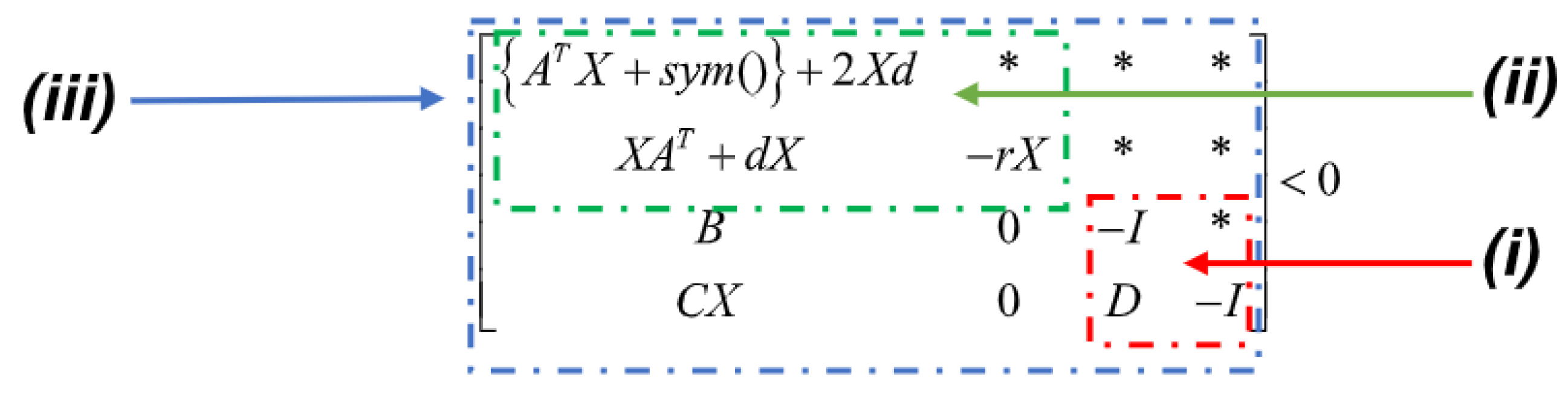
There exists a positive symmetric matrix X such that the following LMI is feasible:

$$\left[\begin{array}{ccc}{A}^{T}X+XA& \ast & \ast \\ B& -I& \ast \\ CX& D& -I\end{array}\right]<0$$

(3)

Proof. 

Based on this configuration is the LMIs expression described by Figure 2.

The condition (i) in Theorem 2 aims to ensure the asymptotic stability of the system over time and to minimize the ratio between the outputs of two successive iterations based on the $H_{\infty }$ optimization problem. The combination leads us to a stability condition along passages described by the condition (ii) given in Theorem 2.

The equivalence between (i) and (ii) is a well-known result.

Note that the third condition of stability along the pass implies that $\rho \left(G\left(s\right)\right)<1\forall \left|s\right|=1$, or if we consider ${\sigma }_{max}$ as the maximum singular value and then the $H_{\infty }$ norm of $G\left(s\right)$$({∥G\left(s\right)∥}_{\infty }={\sigma }_{max}\left(G\left(s\right)\right))$, it is known that ${\sigma }_{max}$ is an upper bound for the eigenvalues modulus of a matrix $\rho \left(G\left(s\right)\right)\le {\sigma }_{max}\left(G\left(s\right)\right)$.

This equality occurs in the MISO case only when $G\left(s\right)$ is a scalar function. Then the LMI of Theorem 2 implies conditions (ii) and (iii) of Theorem 1.

The condition (i) of Theorem 1 is redundant since from the LMI of Theorem 2,we have $\left[\begin{array}{cc}-I& D^T\\ \ast & -I\end{array}\right]<0$, which complete the proof. □

3. Main Results

3.1. Control Objective

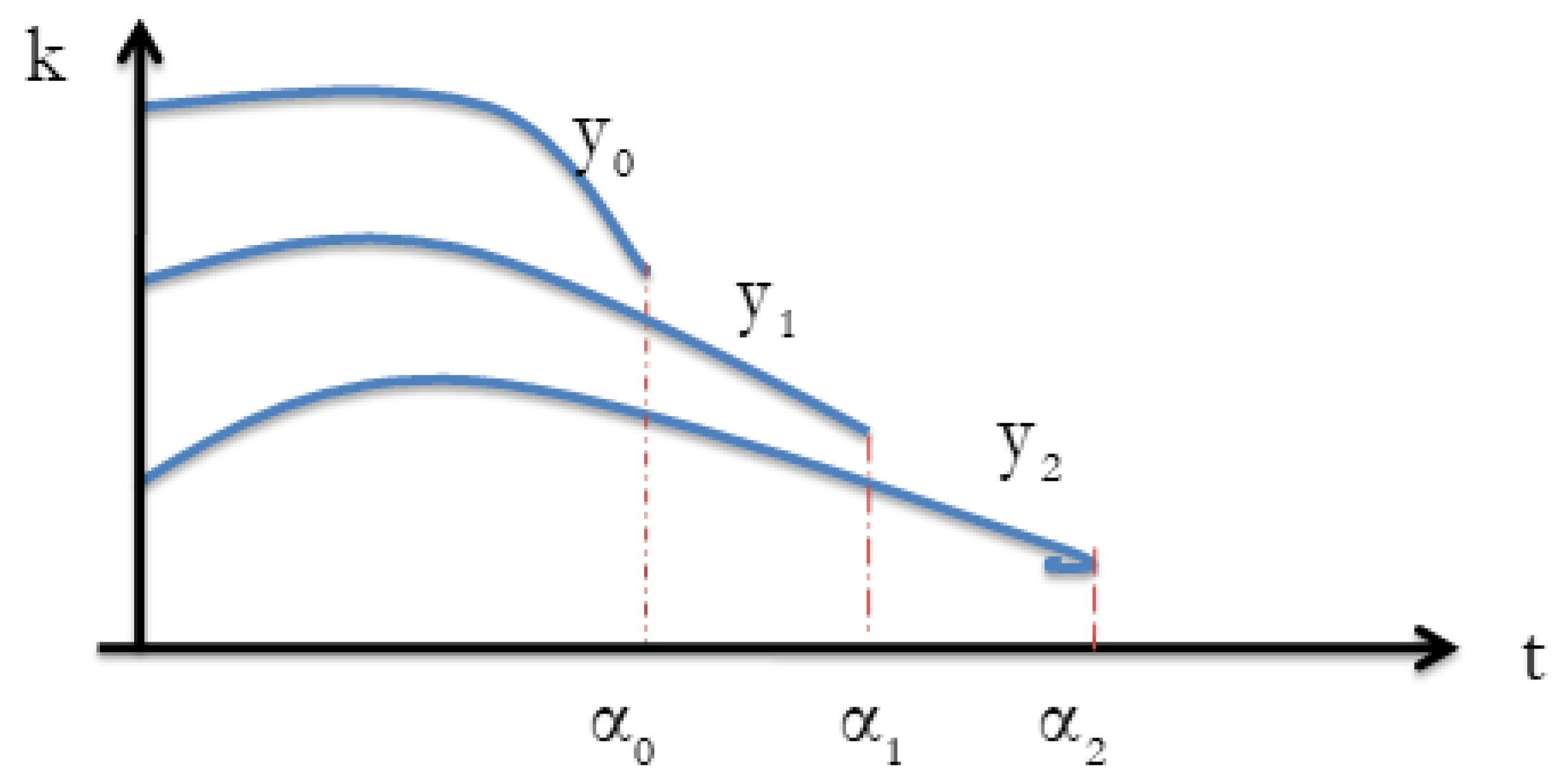
The objective of this section is to transform the problem of stability along the pass of the continuous-time linear repetitive systems into a tracking problem [23].

Consider the following assumptions based on system (1):

• (A1) The desired output $y_d\left(t\right),t=1,\dots ,T$ is given a prior over the same time duration; it is assumed that the initial resetting condition is satisfied, i.e., $y_k\left(0\right)=y_d\left(0\right)$.
• (A2) The initial state remains the same at each iteration, i.e., $x_k\left(0\right)=0,\forall k=1,2,\dots ,N$. For any given assumption A1 and A2, one desirable objective in ILC is that $y_k\left(t\right)$ converges monotonically to $y_d\left(t\right)$ when k tends to infinity for all t within the time interval $\left[0,T\right]$ since it can guarantee reasonable transients during the learning process [3]. In the sense of the, ${\ell }_{2,\left[0,T\right]}$ norm, this objective can be transformed by considering the index [8].

  $$J\left(\gamma ,k\right)=\sum _{t=1}^N\left[{e_{k+1}}^T\left(t\right)e_{k+1}\left(t\right)-{\gamma }^2{e_k}^T\left(t\right)e_k\left(t\right)\right]$$

  (4)

  where $\gamma >0$ is a prescribed scalar and $e_k\left(t\right)$ is the tracking error at the kth iteration, expressed as

  $$e_k\left(t\right)=y_d\left(t\right)-y_k\left(t\right)$$

  (5)
  Obviously, the norm error ${∥e_k\left(t\right)∥}_{2\left[0,T\right]}$ can be guaranteed to converge monotonically along the iteration axis k if $J\left(\gamma \right)<0$ holds for any $\gamma \in \left[0,1\right]$.

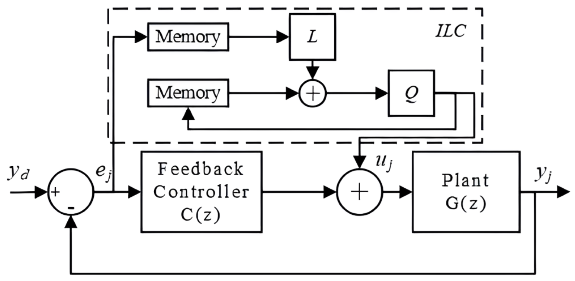
3.2. ILC Tracking Control

In this section, the ILC scheme given by Figure 3 can focus perfectly to overcome the tracking problem when it tracks an iteration’s desired trajectory as k tends to infinity. Following this idea, the concept of the stabilization along the pass can be shown as a tracking problem. The formulated problem is solved by using the iterative learning control described by the following updating ILC law [8]:

$$u_{k+1}\left(t\right)=\beta u_k\left(t\right)+K_1{\dot{\eta }}_{k+1}\left(t\right)+K_2{\dot{e}}_k\left(t\right)$$

(6)

$${\eta }_{k+1}\left(t\right)=\underset{0}{\overset{t}{\int }}(x_{k+1}\left(t\right)-\beta x_k\left(t\right))d\tau {\eta }_k\left(0\right)=0$$

(7)

where ${\eta }_{k+1}\left(t\right)$ denotes the state vector computed to the cycle direction, $K_1,K_2$ are switching learning gains with appropriately dimensioned matrices to be designed, and $\beta$ is a positive scalar to be optimized.

Moreover, if it is assumed that the matrix $D=0$, then clearly, (1) can be written as

$$\left\{\begin{array}{c}{\dot{x}}_k\left(t\right)=A{x}_k\left(t\right)+B{u}_k\left(t\right)\\ y_k\left(t\right)=C{x}_k\left(t\right)\end{array}\right.x\left(0\right)=0,t\ge 0,k>0$$

(8)

(6)–(8) can be written as

$${\dot{\eta }}_{k+1}\left(t\right)=\underset{0}{\overset{t}{\int }}({\dot{x}}_{k+1}\left(t\right)-\beta {\dot{x}}_k\left(t\right))d\tau$$

(9)

$${\dot{\eta }}_{k+1}\left(t\right)=\left(A+B{K}_1\right){\eta }_{k+1}\left(t\right)+B{K}_2{e}_k\left(t\right)$$

$$\beta e_k\left(t\right)-e_{k+1}\left(t\right)=C{\dot{\eta }}_{k+1}\left(t\right)$$

$$e_{k+1}\left(t\right)=-C\left(A_{k+1}+B{K}_1\right){\eta }_{k+1}\left(t\right)+\left(\beta -CB{K}_2\right)e_k\left(t\right)$$

Obviously (8) can be rewritten as

$$\left[\begin{array}{c}{\dot{\eta }}_{k+1}\left(t\right)\\ e_{k+1}\left(t\right)\end{array}\right]=\left[\begin{array}{cc}\left(A+B{K}_1\right)& B{K}_2\\ -C\left(A_{k+1}+B{K}_1\right)& \left(\beta -CB{K}_2\right)\end{array}\right]\left[\begin{array}{c}{\eta }_{k+1}\left(t\right)\\ e_k\left(t\right)\end{array}\right]$$

(10)

The state-space model (10) is that of a continuous linear repetitive process of the form defined by the pass output and state vectors $e_{k+1}\left(t\right)$ and ${\dot{\eta }}_{k+1}\left(t\right)$, respectively.

Note that $T\left(s\right)$ is a transfer matrix between $E_k\left(s\right)$ and $E_{k+1}\left(s\right)$.

From (10) we can obtain

$$E_{k+1}\left(s\right)=T\left(s\right)E_k\left(s\right)$$

(11)

where

$$T\left(s\right)=\left[{\displaystyle \frac{A+B{K}_{1}B{K}_2}{-C\left(A+B{K}_1\right)\left(\beta -CB{K}_2\right)}}\right]$$

(12)

Hence, it can be derived that if ${∥T\left(z\right)∥}_{\infty }<\gamma$, $\gamma \in \left[0,1\right)$ holds, then $\underset{k\to \infty }{lim}{∥e_k\left(t\right)∥}_2=0$ (monotonic convergence in the sense of the norm $l_2$). This implies that although the tracking error over the finite time interval $\left[0,T\right]$ is considered in ILC, the monotonic convergence of the error ${∥e_k\left(t\right)∥}_2$ can also be guaranteed when ${∥T\left(z\right)∥}_{\infty }<\gamma$ is used to obtain the negative performance index $J\left(\gamma \right)<0$.

Theorem 3 

([27]). The output tracking error $e_k\left(t\right)$ converges monotonically to zero when k tends to infinity if and only if the 2D repetitive system (12) is stable along the pass.

Starting from Theorem 3 and by applying the obtained Theorem 2 on the given system representation 12, we can state the following Theorem 4.

Theorem 4 

([23]). The tracking error converges monotonically to zero when k tends to infinity if there exist matrices $K_2,N_1$ and a positive symmetric matrix X and the scalars $\beta ,\gamma \in \left[0,1\right)$, such that the following LMI is feasible:

$$\left[\begin{array}{ccc}\left(AX+B{N}_1\right)+sym(\dots )& \ast & \ast \\ {\left(B{K}_2\right)}^T& -I& \ast \\ -C(AX+B{N}_1)& \beta -CB{K}_2& -{\gamma }^2\end{array}\right]<0$$

(13)

then the gain matrices are given by: $K_2,K_1=N_1{X}^{-1}$.

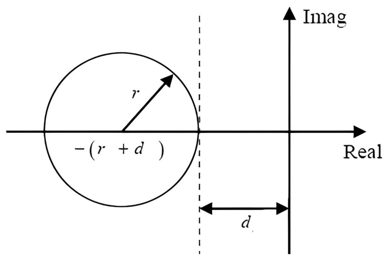
3.3. ILC Tracking Control Using D-Stability along the Pass

In this section, we address the issue of placing all poles of a system within a specified disk, which is commonly known as the D-pole placement problem for continuous-time linear repetitive systems. This method has been devised to control systems that exhibit favorable transient and steady-state responses. Several criteria have been put forth to guarantee that all the closed-loop eigenvalues of continuous-time linear repetitive systems reside within a designated disk $D(-(r+d),r)$ centered at $(-r+d,0)$ with a radius of r, see Figure 4.

Building upon this concept, the tracking control problem utilizing the notion of stabilization along the pass discussed earlier can be depicted as a pole placement problem.

Using the parameter d, it is possible to establish an upper bound for the settling time of the transient response given by $3\tau ,5\tau$ for a repetitive system undergoing the kth iteration, with $\tau ={\displaystyle \frac{1}{d}}$. This value r provides the upper bound on the natural frequency of oscillation for the transient response. Additionally, a lower bound on the damping factor $\xi$, which determines the overshoot, can be computed as follows:

$$\xi ={\displaystyle \frac{\sqrt{\left(r+d\right)-r^2}}{r+d}}$$

(14)

3.4. D-Stability along the Pass for Continuous Linear Repetitive Process

Consider the continuous linear repetitive process having this form over $t\in \left[0,T\right],k\in I{R}_{+}$:

$${\dot{x}}_k\left(t\right)=A{x}_k\left(t\right), x\left(0\right)=0,t\ge 0,k>0$$

(15)

The objective of this section is to establish criteria to ensure that all the eigenvalues of the repetitive system (1) reside within a designated disk $D(-(r+d),r)$ centered at $(-(r+d),0)$ with a radius of r and a distance d from the imaginary axis, as illustrated previously in Figure 4. Initially, we introduce a computationally sufficient condition for ensuring D-stability in repetitive systems. This condition will serve as a fundamental component in deriving ILC tracking control results in the next section.

Theorem 5 

([22]). All the poles of system (15) are located inside a specified disk D centered at $-(r+d)$ with radius r if the following condition is satisfied:

$$\left(A+d\right)X+X{\left(A+d\right)}^T+{\displaystyle \frac{1}{r}}\left(A+d\right)X{\left(A+d\right)}^T<0.$$

(16)

We use the well-known common quadratic Lyapunov function:

$$V_{k+1}\left(x\right)={{\eta }_{k+1}}^{T}P{\eta }_{k+1},P=P^T>0$$

(17)

A sufficient condition such that all the eigenvalues of $(A+BK1)$ of the repetitive system lie inside the circular region $\varsigma \left(d,r\right)$, as depicted in Figure 4, is given by the existence of a positive definite symmetric matrix $X=P^{-1}$ such that the following condition holds.

Theorem 6 

([23]). The tracking error converges monotonically to zero when k tends to infinity if there exist matrices $K_2,N_1$, a positive symmetric matrix X, and the scalars $r>0,d>0,\gamma \in \left[0,1\right),0<\beta <1$ such that the following LMI is feasible:

$$\left[\begin{array}{cccc}\left\{\left(AX+B{N}_1^T\right)+sym(\dots )\right\}+2dX& \ast & \ast & \ast \\ \left(XA+N_1^T{B}^T\right)+dX& -rX& 0& 0\\ {\left(B{K}_2\right)}^T& 0& -I& \ast \\ -C\left(AX+B{N}_1\right)& 0& \left(\beta -CB{K}_2\right)& -{\gamma }^2\end{array}\right]<0$$

(18)

In this case, the gain matrices are given by $K_2,K_1=N_1{X}^{-1}$.

Proof. 

Based on Figure 5, we consider the LMI condition of (13), then replace the bloc diagonal (1, 1) by (16) and apply the Schur complement we obtained (18). □

The objective of the next section is to transform the condition for analyzing D-stability along the passages into a tracking problem using ILC control. This leads to a new interpretation of Theorem 6.

3.5. Polynomial ILC Control

This section builds upon the idea introduced in the previous section, where the concept of D-stabilization along the pass is framed as a tracking problem utilizing high-order iterative learning control.

The methodology for designing the iterative learning control (ILC) law, particularly in the context of polynomial-based approaches such as Poly-ILC, involves several key steps and considerations: modeling the system and defining the control law, learning mechanism, and iterative optimization. The rationale behind the choice of polynomial-based approaches like Poly-ILC lies in their flexibility and adaptability. Polynomial functions offer a versatile framework for representing complex trajectories and can capture a wide range of desired behaviors with relatively few parameters. Additionally, polynomial-based approaches provide smooth and continuous control signals, which can be advantageous for systems with continuous dynamics. Specific contributions of Poly-ILC include the following:

• Introducing a novel polynomial-based approach to iterative learning control, which offers a flexible and intuitive framework for defining desired trajectories.
• Advancing existing techniques by providing a systematic methodology for designing and optimizing polynomial-based control laws for repetitive systems.
• Demonstrating improved tracking performance and robustness compared to traditional ILC methods, particularly in applications with complex and time-varying dynamics. Overall, Poly-ILC represents a significant advancement in the field of iterative learning control, offering a powerful and versatile approach for achieving accurate and reliable tracking in repetitive systems.

We consider a control law in the following form over $t\in \left[0,T\right]$ and $k\in {\mathbf{N}}_{+}$:

$$u_{k+1}\left(t\right)=v_{k+1}\left(t\right)+L_1{x}_{k+1}\left(t\right)$$

(19)

Applying the control law (19) to system (8), the following state space is then obtained:

$$\left\{\begin{array}{c}{x}_{k+1}\left(t+1\right)=\left(A+B{L}_1\right)x_{k+1}\left(t\right)+B{v}_{k+1}\left(t\right)\hfill \\ y_{k+1}\left(t\right)=C{x}_{k+1}\left(t\right)\hfill \end{array}\right.$$

(20)

where $t\in \left[0,T\right]$, $k=0,1,\dots ,N$.

Obviously, from (20), the transfer function matrix from $u_{k+1}\left(t\right)$ to $y_{k+1}\left(t\right)$ can be expressed as

$$Y_{k+1}\left(s\right)=G\left(s\right)U_{k+1}\left(s\right)$$

(21)

where

$$G\left(z\right)=C{\left(sI-A+B{L}_1\right)}^{-1}B$$

(22)

Now, we introduce the polynomial ILC law as follows:

$$V_{k+1}\left(s\right)=\beta V_k\left(s\right)+L_2\left(s\right)E_k\left(s\right)$$

(23)

$$L_2\left(s\right)=\sum _{q=0}^r{L}_{2,q}{s}^q$$

(24)

where the Laplace transform of the form $E_k\left(z\right)=Z\left[e_k\left(t\right)\right]$, $L_2\left(s\right)$ is a polynomial learning gain matrix to be designed, and r is the degree of the learning controller $L_2\left(s\right)$.

Given the system (20) with updating structure of control (23), and verifying assumptions A1 and A2, we find appropriate learning controller $L_2\left(s\right)$ such that the robust monotonic convergence of $e_k$ is achieved and the output error $e_k\left(t\right)$ for $t=1,\dots ,T$ converges to zero as $k\to \infty$. Therefore, let us express the difference error as

$$e_{k+1}\left(t\right)-e_k\left(t\right)=-\left(y_{k+1}\left(t\right)-y_k\left(t\right)\right)$$

(25)

Consequently, the Laplace transform of the difference between errors at iterations takes the following form:

$$E_{k+1}\left(s\right)-E_k\left(s\right)=-\left(Y_{k+1}\left(s\right)-Y_k\left(s\right)\right)$$

(26)

$$E_{k+1}\left(s\right)-E_k\left(s\right)=-G\left(s\right)\left(U_{k+1}\left(s\right)-U_k\left(s\right)\right)$$

(27)

$$E_{k+1}\left(s\right)-E_k\left(s\right)=-G\left(s\right)L_2\left(s\right)E_k\left(s\right)$$

(28)

This leads to

$$E_{k+1}\left(s\right)=\left(I-G\left(s\right)L_2\left(s\right)\right)E_k\left(s\right)$$

(29)

Based on the preceding developments, deriving a condition for the monotonic convergence of the ILC systems (20) and (21) is straightforward.

$$E_{k+1}\left(s\right)=\left[\beta -C{\left(sI-\left(A+B{L}_1\right)\right)}^{-1}B\sum _{q=0}^r{L}_{2,q}{s}^q\right]E_k\left(s\right)$$

(30)

Let us use the transfer matrix defined by

$$T\left(s\right)=\beta -C{\left(sI-\left(A+B{L}_1\right)\right)}^{-1}B\sum _{q=0}^r{L}_{2,q}{s}^q$$

(31)

Note that with the relative degree of the polynomial controller $r=1$, building upon Equation (31), we arrive at this result:

$$T\left(s\right)=\beta -C{\left(sI-\left(A+B{L}_1\right)\right)}^{-1}B\left[L_{21}+s{L}_{22}\right]$$

(32)

Considering the fact that

$$s{\left(sI-A\right)}^{-1}=I+A{\left(sI-A\right)}^{-1}$$

It results that

$$\begin{array}{c}T\left(s\right)=-C{\left(sI-\left(A+B{L}_1\right)\right)}^{-1}\left[\left(B{L}_{21}+\left(A+B{L}_1\right)B{L}_{22}\right)\right]+\left(\beta -CB{L}_{22}\right)\hfill \end{array}$$

(33)

If there exist matrices $\tilde{A},\tilde{B},\tilde{C},\tilde{D}$, we can written $T\left(s\right)$ as

$$\begin{array}{c}T\left(s\right)=\tilde{C}{\left(sI-\tilde{A}\right)}^{-1}\tilde{B}+\tilde{D}\hfill \\ :=\left[\left.{\displaystyle \frac{\tilde{A}}{\tilde{C}}}\right|{\displaystyle \frac{\tilde{B}}{\tilde{D}}}\right]\hfill \end{array}$$

(34)

Referring to (34), $T\left(s\right)$ can be written as follows:

$$T\left(s\right):=\left[\left.{\displaystyle \frac{\left(A+B{L}_1\right)}{-C}}\right|{\displaystyle \frac{\left(B{L}_{21}+\left(A+B{L}_1\right)B{L}_{22}\right)}{\beta -CB{L}_{22}}}\right]$$

(35)

Now, we introduce LMI conditions aimed at ensuring the monotonic convergence of P-ILC. Considering the performance index $J\left(\gamma \right)$ and applying the BRL relative to robust $H_{\infty }$ control theory [28,29], Theorem 7 is as follows.

Theorem 7.

The tracking error converges monotonically to zero when k tends to infinity if there exist matrices $L_{21},L_{22},N,G$, a positive symmetric matrix X, and the scalars $r>0,d>0,\gamma \in \left[0,1\right),0<\beta <1,0<\alpha <1$ such that the following LMI is feasible:

$$\left[\begin{array}{ccccc}2\left(d-\alpha \right)X& \ast & \ast & \ast & \ast \\ \left(d-\alpha \right)X& -rX& 0& 0& \ast \\ {\left(B{L}_{21}\right)}^T-\alpha B{L}_{22}& 0& -I& \ast & \ast \\ -CX& 0& \left(\beta -CB{L}_{22}\right)& -{\gamma }^2& \ast \\ \left(G{A}^T+N^T{B}^T\right)+\alpha G^T+X^T& X^T& B{L}_{22}& 0& -G-G^T\end{array}\right]<0$$

(36)

Then $L_1=N{X}^{-1}$.

Proof. 

Substitute the new model (35) in this LMI, guaranteeing the ILC tracking control using D-stability along the pass of theorem (6).

We obtain this LMI:

$$\left[\begin{array}{cccc}\left(A+B{L}_1\right)X+X{\left(A+B{L}_1\right)}^T+2dX& \ast & \ast & \ast \\ X{\left(A+B{L}_1\right)}^T+dX& -rX& 0& 0\\ {\left(B{L}_{21}\right)}^T+{\left(B{L}_{22}\right)}^T{\left(A+B{L}_1\right)}^T& 0& -I& \ast \\ -CX& 0& \left(\beta -CB{L}_{22}\right)& -{\gamma }^2\end{array}\right]<0$$

(37)

We rewrite (37) as

$$\left[\begin{array}{cccc}2dX-2\alpha X& \ast & \ast & \ast \\ dX-\alpha X& -rX& 0& 0\\ {\left(B{L}_{21}\right)}^T-\alpha B{L}_{22}& 0& -I& \ast \\ -CX& 0& \left(\beta -CB{L}_{22}\right)& -{\gamma }^2\end{array}\right]+\left\{\left[\begin{array}{c}\left(A+B{L}_1\right)+\alpha I\\ 0\\ 0\\ 0\end{array}\right]\left[\begin{array}{cccc}X& X& B{L}_{22}& 0\end{array}\right]+sym\left\{\dots \right\}\right\}<0$$

(38)

Furthermore, applying the projection lemma for inequality (38), the inequality (36) is obtained. This end the proof. □

4. Uncertain LRP Systems

4.1. Problem Formulation

In most synthesis problems, the desired objective is to achieve and maintain specific robust performance goals despite the often detrimental uncertainties of the system to be controlled. To demonstrate the robustness of the ILC (iterative learning control) used, we consider the LRP system (1) with polytopic modeling uncertainties.

$$\left\{\begin{array}{c} {\dot{x}}_k\left(t\right)=\widehat{A}{x}_k\left(t\right)+\widehat{B}{u}_k\left(t\right)\\ y_k\left(t\right)=\widehat{C}{x}_k\left(t\right)+\widehat{D}{u}_k\left(t\right)\end{array}\right.x_k\left(0\right)=0,t\ge 0,k>0$$

(39)

Such matrices as $\widehat{A}$ and $\widehat{B},\widehat{C},\widehat{D}$ are sets of matrices defined by

$$\left\{\widehat{A}=\sum _{i=1}^{N_A}{\theta }_i{A}_i,\sum _{i=1}^{N_A}{\theta }_i=1,{\theta }_i\ge 0\right\}$$

(40)

$$\left\{\widehat{B}=\sum _{i=1}^{N_B}{\theta }_i{B}_i,\sum _{i=1}^{N_B}{\theta }_i=1,{\theta }_i\ge 0\right\}$$

(41)

$$\left\{\widehat{C}=\sum _{i=1}^{N_C}{\theta }_i{C}_i,\sum _{i=1}^{N_C}{\theta }_i=1,{\theta }_i\ge 0\right\}$$

(42)

$$\left\{\widehat{D}=\sum _{i=1}^{N_D}{\theta }_i{D}_i,\sum _{i=1}^{N_D}{\theta }_i=1,{\theta }_i\ge 0\right\}$$

(43)

where $N_A$, $N_B$, $N_C$, and $N_D$ are the number of vertices of the polytopes.

4.2. Poly-Quadratic Stability

The concept of a robust ILC synthesis method is based on the polyquadratic approach. This approach relies on the use of a Lyapunov function that depends on uncertain parameters. These functions enable the analysis of stability and stabilization of continuous-time LRP systems. We consider the LRP system described by Equation (39). The system modeling involves the use of Lyapunov functions that depend on uncertain parameters.

Let

$$V_i\left(k,t\right)=x^T\widehat{P}x$$

(44)

$$V_i\left(k,t\right)=x^T\sum _{i=1}^{N_D}{\theta }_i{P}_{i}x$$

(45)

$$\widehat{P}=\sum _{i=1}^{N_P}{\theta }_i{P}_i$$

(46)

where k describes the evolution of the Lyapunov function at the $k^{eme}$ iteration and $N_P$ is the number of vertices of the polytope.

Theorem 8.

Consider the uncertain repetitive LRPs system (39) in a closed loop. The system is D-stable along the pass and the tracking error $e_{k+1}\left(t\right)$ converges monotonically to zero as k tends to infinity if there exist scalars $\gamma ,\alpha ,r,d$, matrices $K_{2,i}$, $N_i$, and positive symmetric matrices $G_i$ such that the following optimization problem is feasible:

$$\begin{array}{c}\underset{0<\gamma ,\alpha <1}{min\left(\gamma ,\alpha \right)}\hfill \\ \left[\begin{array}{cccc}\left\{A_i^T{G}_i+N_i^T{B}_i^T+sym\left(\dots \right)\right\}+2G_{i}d& \ast & \ast & \ast \\ A_i^T{G}_i+N_i^T{B}_i^T+d{G}_i& -r{G}_i& \ast & \ast \\ K_{2,i}^T{B}_i^T& 0& -I& \ast \\ -C_i{A}_i{G}_i-C_i{B}_i{N}_i& 0& \alpha -C_i{B}_i{K}_{2,i}& -{\gamma }^2\end{array}\right]<0\hfill \end{array}$$

(47)

Then the learning gains are given by the following:

For $i=1\dots N_A$,

$$K_{2,i},K_{1,i}=N_i{G}_i^{-1}.$$

The construction of a robust ILC synthesis method is based on the polyquadratic approach. This approach requires the use of a Lyapunov function dependent on the uncertain parameters. The system with LRP described by Equation (39) is considered. The modeling of the system necessitates the use of Lyapunov functions that depend on the uncertain parameters. Theorem 8 is an extension of the results to the case of polytopic uncertainty, using polytopic Lyapunov functions.

5. Numerical Examples

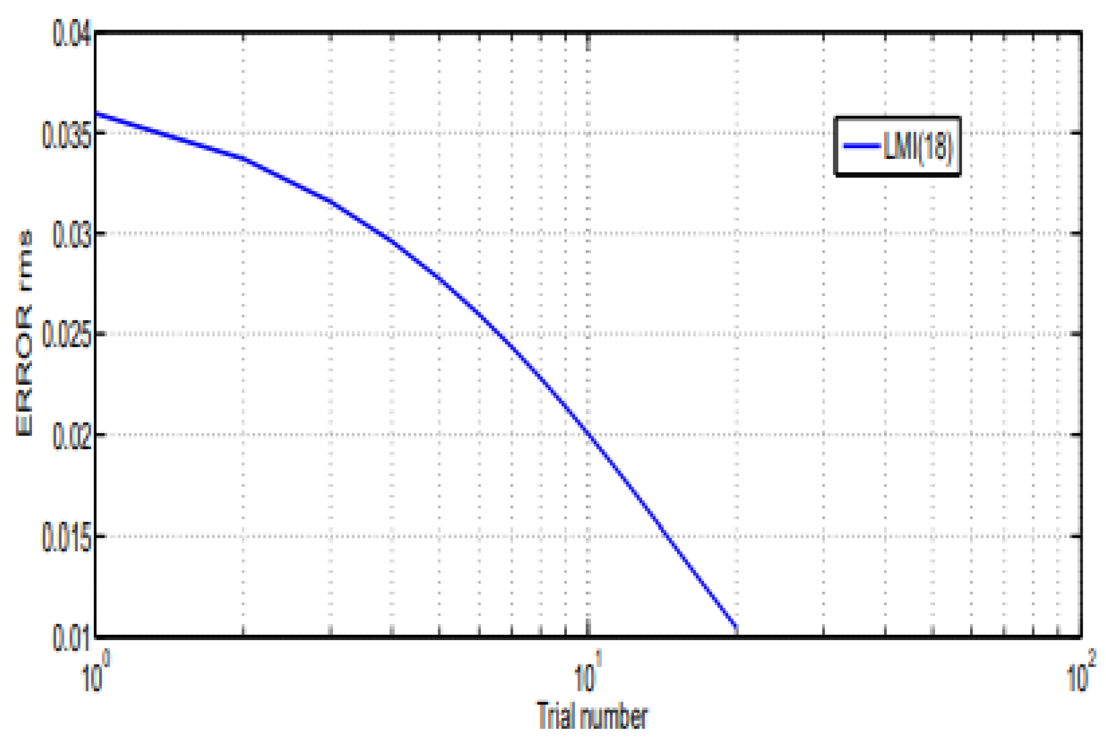
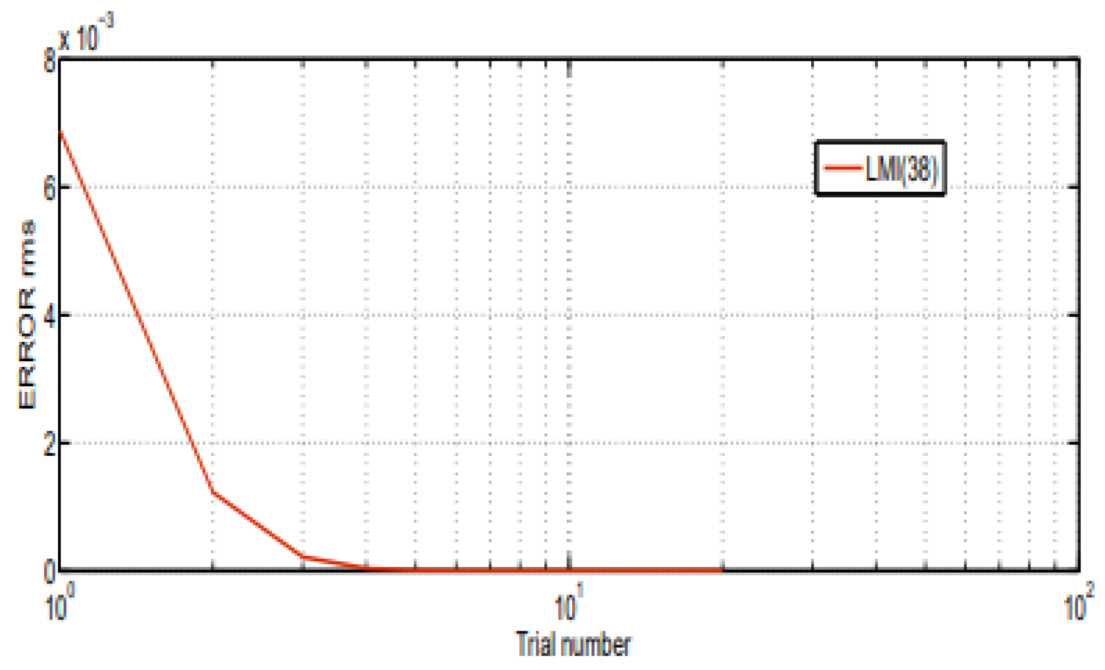
5.1. Comparison between D-ILC Tracking Control and D-Poly-ILC Tracking Control

In this section, the effectiveness of the proposed design methods is demonstrated through simulation results utilizing MATLAB software. Consider the active suspension system of a car, as shown in Figure 6. All details regarding the system behavior and operation can be found in [20]. The matrices of the model (1) are presented as follows:

The model consists of a car mass $M_c$ and a driver seat mass $m_s$. Vertical vibrations caused by a road can be partially attenuated by the stiffness $k_1$ and damping $b_1$ of the shock absorbers. The driver may still experience undesirable vibrations, which can be reduced by seat suspension elements of stiffness $k_2$ and damping $b_2$. Damping of the vibrations of $M_c$ and $m_s$ can be increased by changing the control inputs $u_1$ and $u_2$.

$A=\left[\begin{array}{cccc}0& 1& 0& 0\\ 0& 0& 0& 1\\ {\displaystyle \frac{-k_1-k_2}{M_c}}& {\displaystyle \frac{k_2}{M_c}}& {\displaystyle \frac{-b_1-b_2}{M_c}}& {\displaystyle \frac{b_2}{M_c}}\\ {\displaystyle \frac{k_2}{m_s}}& -{\displaystyle \frac{k_2}{m_s}}& {\displaystyle \frac{b_2}{m_s}}& -{\displaystyle \frac{b_2}{m_s}}\end{array}\right]$, $B=\left[\begin{array}{cc}0& 0\\ 0& 0\\ {\displaystyle \frac{1}{M_c}}& -{\displaystyle \frac{1}{M_c}}\\ 0& {\displaystyle \frac{1}{m_s}}\end{array}\right];C=\left[\begin{array}{cccc}0& 1& 0& 0\end{array}\right].$ with the following: ${\mathrm{M}}_{\mathrm{c}}=1500\mathrm{kg}$, ${\mathrm{m}}_{\mathrm{s}}=90\mathrm{kg}$, ${\mathrm{k}}_1=4\times {10}^4\mathrm{N}/\mathrm{m}$, ${\mathrm{k}}_2=5\times {10}^3\mathrm{N}/\mathrm{m}$, ${\mathrm{b}}_1=4\times {10}^3\mathrm{Ns}/\mathrm{m}$, ${\mathrm{b}}_2=5\times 10^2\mathrm{Ns}/\mathrm{m}$.

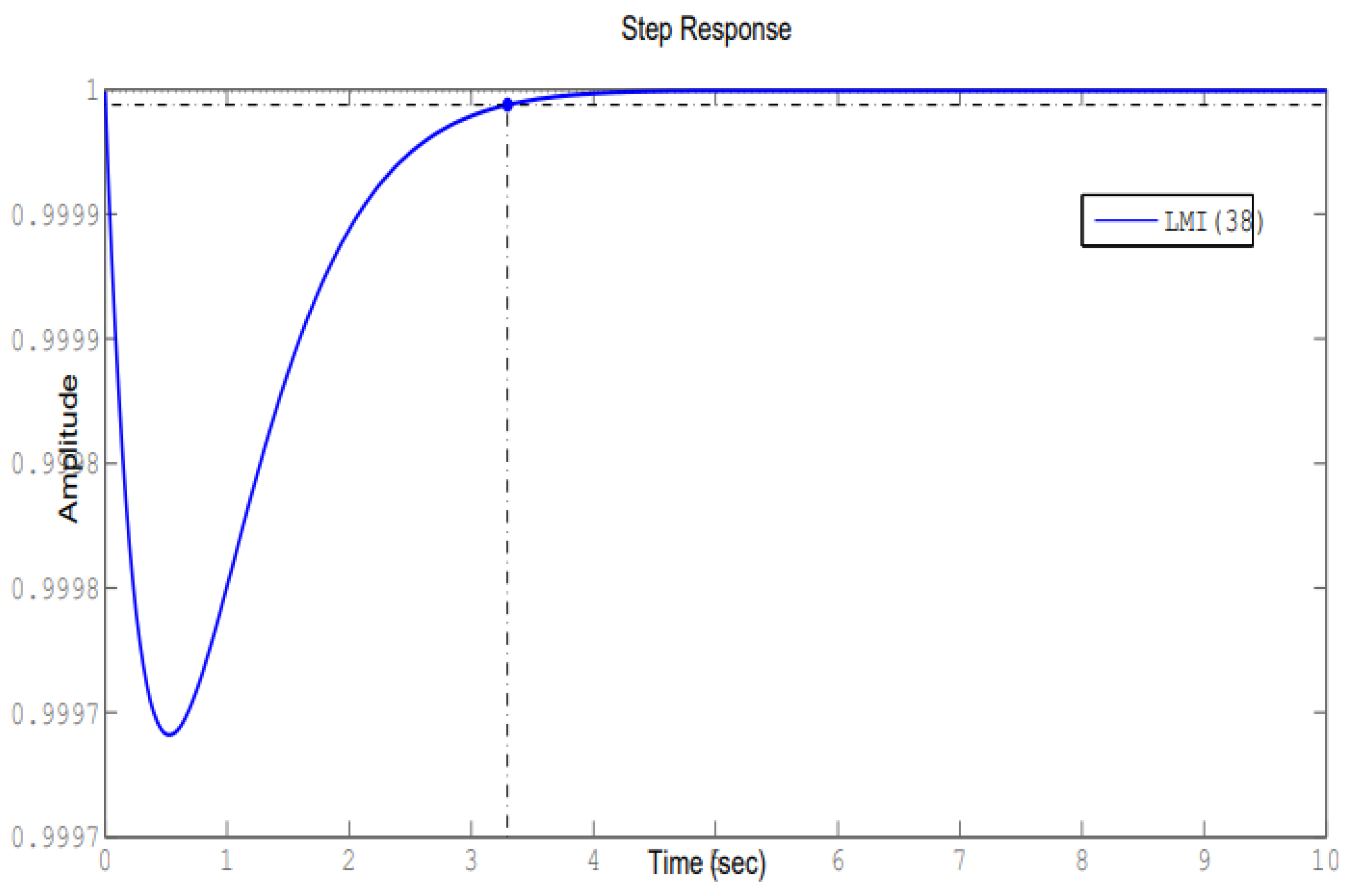
5.1.1. ILC Controller for Desired Performances

The primary objective is to ensure certain step response performances such as settling time and overshoot. Based on Theorems 6 and 7, and by solving the set of LMIs (18) and (36), the system under consideration is monotonically stabilized by designing learning gains with the following desired performances:

• Overshoot $\le 5\%$.
• Setting time at $2\%\le 10\%$.

Therefore, it can be inferred that the proposed approach implements D-pole assignment, and the pole locations within the specified disk D are applied for $r=1$ and $d=0.685$. In this scenario, the computed learning gains are provided in

Table 1. Proposed approaches.

Parameters	Approaches	Learning Gains
$\beta =0.99$
$\gamma =0.99$	Theorem 6	$K_1=\left[\begin{array}{cccc}2.25& 0.25& 0.041& 0.753\\ -0.52& 0.451& -0.050& 0.013\end{array}\right]\times {10}^4$
		$K_2=\left[\begin{array}{c}23.02\\ 0.072\end{array}\right]$
$\beta =0.99$
$\gamma =0.99$
$\alpha =0.75$	Theorem 7	$L_1=\left[\begin{array}{cccc}4.007& 0.01& 0.15& -0.029\\ -0.53& 0.44& -0.55& 0.008\end{array}\right]\times {10}^4$
		$L_{21}=\left[\begin{array}{c}0.74\\ 0.09\end{array}\right]$
		$L_{22}=\left[\begin{array}{c}0.83\\ 0.12\end{array}\right]$

:

The closed-loop response achieved with the obtained controller as depicted in Figure 7 illustrates comparable desired specifications defined by the ILC Theorem 6 and the Polynomial-type ILC Theorem 7. Therefore, the resulting ILC process using the D-stability along the pass formulation can ensure a settling time of less than 10 s with no overshoot compared to the desired value previously listed. As is evident from Figure 8, when we opt for identical values of d and r for both LMIs given by Theorem 6 and Theorem 7, we can assess the effectiveness of polynomial ILC control in ensuring the desired system specifications. However, we will later demonstrate the impact of the slack parameter $\alpha$ on enhancing the desired system specifications while keeping d and r constant and varying $\alpha$.

In Figure 9, where $\alpha >0.75$, the designed polynomial ILC proves to be highly effective in guaranteeing a critical system performance.

The achieved results are demonstrated in

Table 2. Polynomial-ILC approach.

Parameters	Approach	Learning Gains
$\beta =0.99$
$\gamma =0.99$	Theorem 7	$L_1=\left[\begin{array}{cccc}2.25& 0.27& 0.16& -0.02\\ -0.52& 0.43& -0.55& 0.008\end{array}\right]\times {10}^4$
		$L_{21}=\left[\begin{array}{c}5.93\\ 0.072\end{array}\right]$
		$L_{22}=\left[\begin{array}{c}6.2\\ 0.1\end{array}\right]$

.

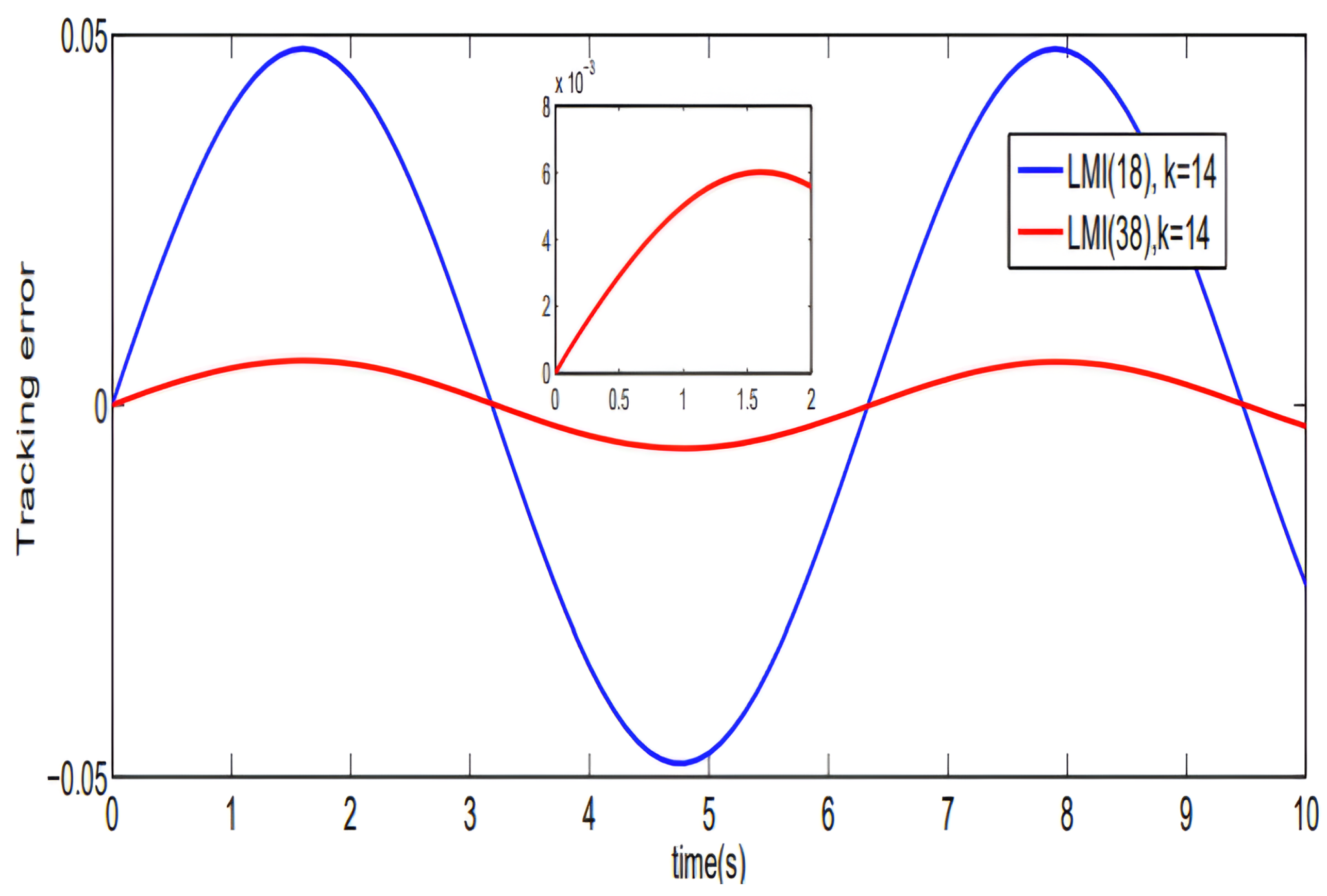
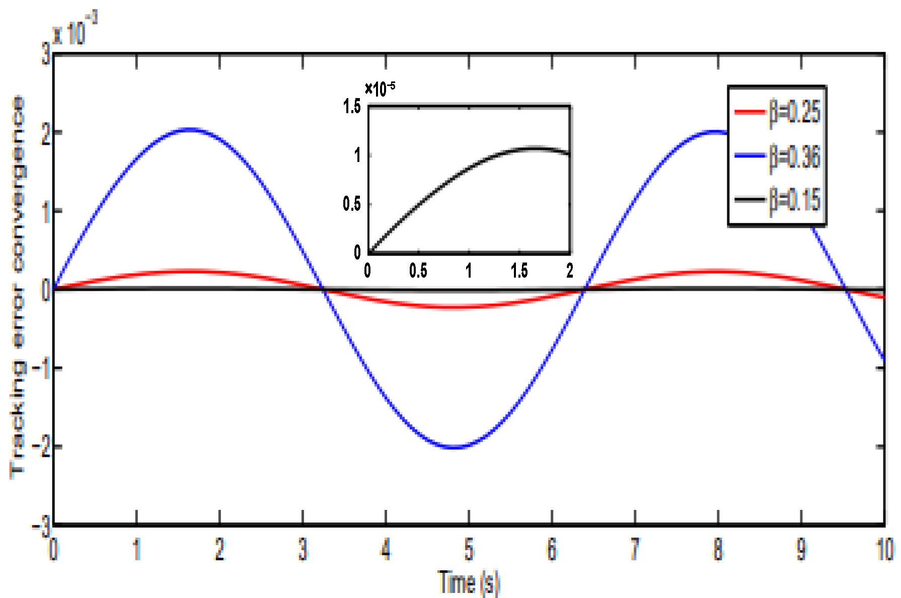
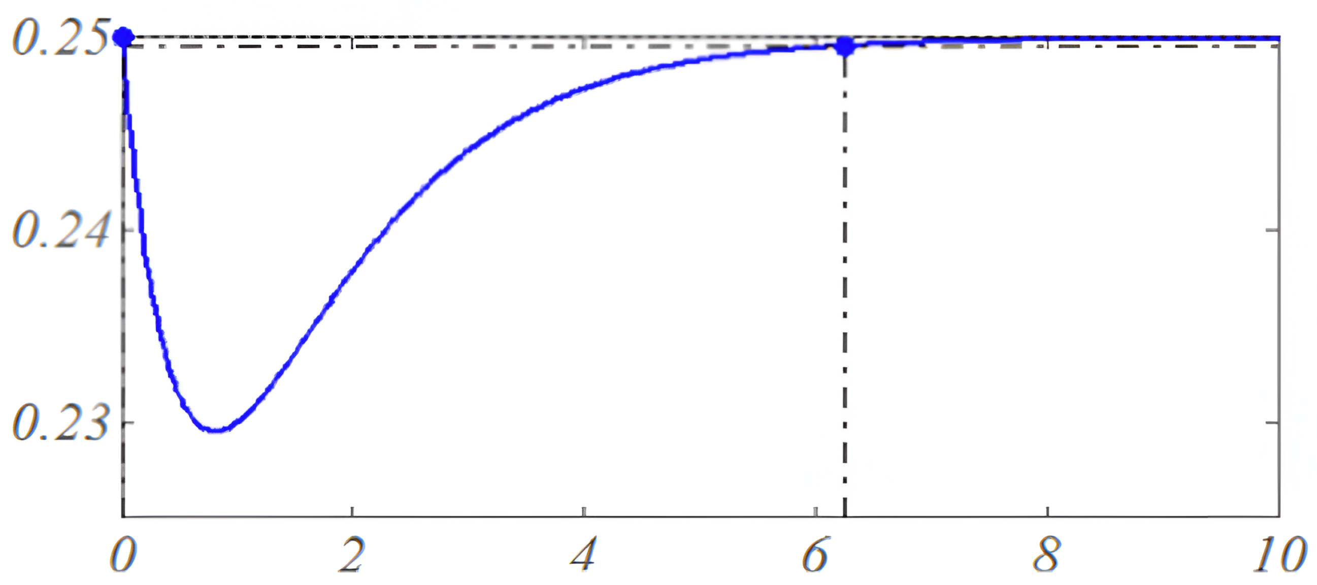
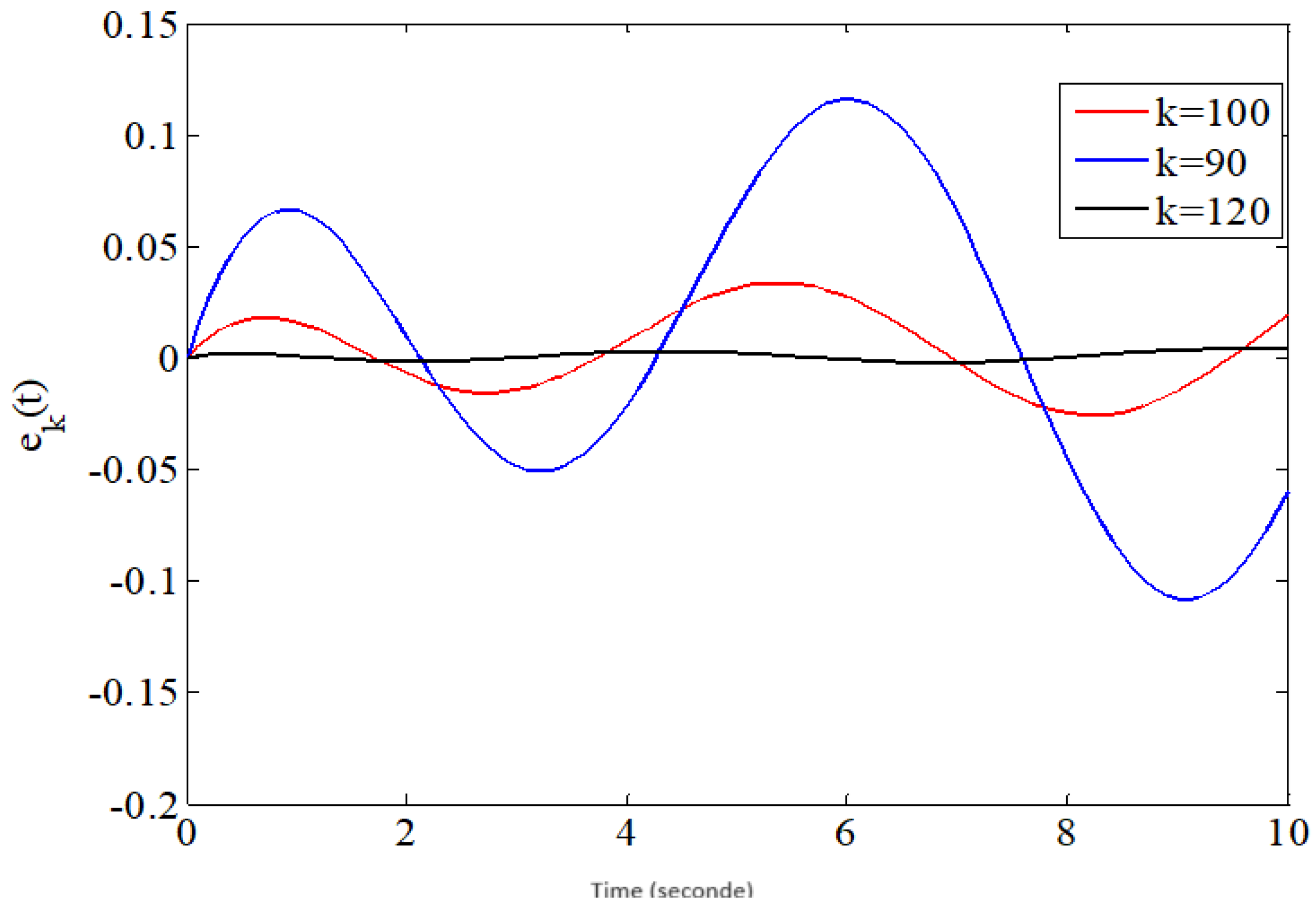
5.1.2. Tracking Error Convergence

In the sequel, consider the linear system (1). For this purpose, the desired trajectory is defined as follows:

$$y_d\left(t\right)=sin\left(t\right),t\in \left[0,10\right]$$

(48)

Initially, Figure 10 illustrates the evolution of the tracking error in relation to the iteration number for $k=14$ for the ILC schemes.

Subsequently, Figure 11 depicts comparable tracking errors generated by the polynomial-type ILC (7) and ILC (6). Consequently, the resulting ILC process ensures that its tracking error converges to zero along the iteration axis. The root mean square error is defined by the following equation:

$$e_{RMS}=\sqrt{{\displaystyle \frac{1}{\alpha }}\sum _{p=0}^{\alpha -1}{e}_k^T\left(p\right)e_k\left(p\right)}$$

(49)

Additional quantitative information can be extracted from Figure 12, Figure 13 and Figure 14, which display the root mean square (RMS) values of the tracking errors. The convergence of error from pass to pass is evaluated using the RMS error for both the polynomial-type ILC law and the proportional ILC.

5.1.3. Discussion

In theorem (7), the pass-to-pass updating error is represented by $e_{k+1}\left(t\right)=\phi e_k\left(t\right)$, where $\phi$ is a bounded linear matrix operator. The property of convergence error between the different profiles along the iteration domain requires the existence of finite real scalars $\phi \in \left[0,1\right)$ such that $∥e_{k+1}\left(t\right)∥\le \phi e_k\left(t\right)$. This prompts a discussion on the speed of convergence error after the iteration number as a function of $\phi$ such as

$$\phi =\beta -CB{L}_{22}$$

(50)

The relaxed parameters $\beta$ play a crucial role in ensuring the monotonic speed convergence of the system with the minimum number of iterations, illustrated by

Table 3. The speed convergence error.

$\mathit{\beta }$	$\mathit{\gamma }$	$\mathit{\alpha }$	$\mathit{\phi }$
0.36	0.9	0.9	0.3503
0.25	0.9	0.9	0.232
0.15	0.9	0.9	0.148

.

On the contrary, Figure 15 illustrates the evolution of the tracking error for different values of $\beta$ as listed in Table 3.

The main contribution consists of developing a new stability condition, which achieves the convergence of the error to zero, and solving the tracking error problem by applying a D-Poly-ILC control for continuous repetitive systems. The synthesis problem of the robust ILC produces 2D repetitive continuous systems. The derived conditions are expressed as a family of linear matrix inequalities (LMIs) parameterized by the scalar variables ${\beta }_{opt}$ and ${\gamma }_{opt}$. These conditions reduce significantly the conservatism and the speed convergence of error and show the advantage of using the scalar variables in the case of ILC control.

5.2. Uncertain Case

For certain situations, we can consider the case where the stiffness of the spring adjustment mechanism and the hardness of the metal strip can degrade after some time. To account for this latter configuration, we consider uncertainties on both parameters ${\lambda }_1,{\lambda }_2$ with ${\lambda }_1\in \left[{\lambda }_{1min},{\lambda }_{1max}\right]$ = [550, 676] and ${\lambda }_2\in \left[{\lambda }_{2min},{\lambda }_{2max}\right]=[1924,2178]$.

In this case, the state matrices (39) of Figure 6 transform into an uncertain polytopic model with four polytopes, with

$$A_1=\left[\begin{array}{cc}0& 1\\ -0.427& 0\end{array}\right], B_1=\left[\begin{array}{c}0\\ -0.002\end{array}\right]$$

$$A_2=\left[\begin{array}{cc}0& 1\\ -0.5006& 0\end{array}\right], B_2=\left[\begin{array}{c}0\\ -2.29\times {10}^{-4}\end{array}\right]$$

$$A_3=\left[\begin{array}{cc}0& 1\\ -0.439& 0\end{array}\right], B_3=\left[\begin{array}{c}0\\ -2.015\times {10}^{-4}\end{array}\right]$$

$$\begin{array}{c}{A}_4=\left[\begin{array}{cc}0& 1\\ -0.50024& 0\end{array}\right], B_4=\left[\begin{array}{c}0\\ -2.6\times {10}^{-4}\end{array}\right]\hfill \\ C=\left[\begin{array}{cc}1& 0\end{array}\right]\hfill \end{array}$$

The objective in this case is to determine the matrices $K_{1,i}$ such that the spectrum of $\widehat{A}$ belongs to a region D for any ${\theta }_i\in N_A$. Furthermore, the varying gain matrices are given by

$$K_{1,1}=\left[\begin{array}{cc}-3.5734& -2.2572\end{array}\right]$$

$$K_{1,2}=\left[\begin{array}{cc}0.4056& -0.2578\end{array}\right]{10}^{-3}$$

$$K_{1,3}=\left[\begin{array}{cc}0.0273& 0.0314\end{array}\right]$$

$$K_{1,4}=\left[\begin{array}{cc}0.4523& -0.2858\end{array}\right]{10}^{-3}$$

For

$$r=1, d=0.83$$

Figure 16 shows the step response of the uncertain closed-loop system for $({\alpha }_{opt}=0.94$, ${\gamma }_{opt}=0.95)$ with a response time of $t_r=6.32$ s and an overshoot of $\pm 5\%$ equal to 0.00102.

Convergence of the tracking error: Based on the theoretical approach proposed in Theorem 8, it is evident from Figure 17 that the tracking error $e_k$ converges to zero after a certain number of iterations. The tracking errors are obtained using varying tracking gains depending on the polytopes.

$$K_{2,1}=-2.4448, K_{2,2}=0.1151, K_{2,3}=0.1743, K_{2,4}=0.0713$$

In this final part, an extension of the results to the case of polytopic uncertainties is considered, using polyquadratic Lyapunov functions as the theoretical foundation.

6. Conclusions

This paper presents significant new findings regarding the ILC-tracking problem for 2D repetitive systems. Specifically, it demonstrates that the three conditions of stability along the iteration can potentially be replaced by a quadratic necessary and sufficient condition. This condition ensures the improvement of performance for repetitive systems and addresses the tracking error problem for this category of systems simultaneously. The primary contribution lies in proposing a new LMI condition that both achieves the convergence of the error to zero and ensures the desired specifications of the transient response of the repetitive system. By transforming the tracking problem with the real bounded lemma into an optimization problem using a variable-introducing control law, a degree of freedom is provided to ensure the feasibility of a stabilizing margin and guaranteeing the adjustment of the system’s poles from one iteration to another using the concept of a stability disk known as “D-stability along the pass”. The results demonstrate the usefulness of ILC in reducing the tracking error. Finally, the effectiveness of the proposed approach is validated through numerical examples.

References

1. Arimoto, S.; Kawamura, M. Bettering operations of robots by learning. J. Robot. Syst. 1984, 2, 123–140. [Google Scholar] [CrossRef]
2. Paszke, W.; Galkowski, K.; Rogers, E. Repetitive process based iterative learning control design using frequency domain analysis. In Proceedings of the IEEE Multi-Conference on Systems and Control, Dubrovnik, Croatia, 3–5 October 2012; pp. 3–6. [Google Scholar]
3. Rogers, E.; Galkowski, K.; Owens, D.H. Control Systems Theory and Applications for Linear Repetitive Processes; Springer Science & Business Media: Berlin/Heidelberg, Germany, 2007; pp. 96–140. [Google Scholar]
4. Hmamed, A.; Alfidi, M.; Benzaouia, A.; Tadeo, F. LMI conditions for robust stability of 2D linear discrete-time systems. Math. Probl. Eng. 2008, 2008, 356124. [Google Scholar] [CrossRef]
5. Mansouri, B.; Manamanni, N.; Guelton, K.; Kruszewski, A.; Guerra, T.M. Output feedback LMI tracking control conditions with H1 criterion for uncertain and disturbed T-S models. Inf. Sci. 2011, 179, 393–414. [Google Scholar]
6. Wu, L.; Su, X.; Shi, P. Mixed H2/H approach to fault detection of discrete linear repetitive processes. J. Frankl. Inst. 2011, 348, 393–414. [Google Scholar] [CrossRef]
7. Paszke, W.; Bachelier, O. New Robust stability and stabilization conditions for linear repetitive processes. In Proceedings of the International Workshop on Multidimensional (nD) Systems, Thessaloniki, Greece, 29 June–1 July 2009; pp. 1–6. [Google Scholar]
8. Van De Wijdeven, J.J.M.; Donkers, M.C.F.; Bosgra, O.H. Iterative learning control for uncertain systems: Non causal finite time interval robust control design. Int. J. Robust Nonlinear Control. 2011, 21, 1645–1666. [Google Scholar] [CrossRef]
9. Paszke, W. Analysis and synthesis of multidimensional system classes using linear matrix inequality methods. In Lecture Notes in Control and Computer Science, Volume 8; Springer: Berlin/Heidelberg, Germany, 2005; pp. 2298–2302. [Google Scholar]
10. Chen, Y.; Wen, C.; Sun, M. A robust high-order P-type iterative learning controller using current iteration tracking error. Int. J. Control 1997, 68, 331–342. [Google Scholar] [CrossRef]
11. Li, B.; Riaz, S.; Zhao, Y. Experimental Validation of Iterative Learning Control for DC/DC Power Converters. Energies 2023, 16, 6555. [Google Scholar] [CrossRef]
12. Jiang, Z.; Chu, B. Norm Optimal Iterative Learning Control: A Data-Driven Approach. IFAC 2022, 55, 482–487. [Google Scholar] [CrossRef]
13. Wei, Y.S.; Yang, X.; Shang, W.; Chen, Y.Y. Higher-Order Iterative Learning Control with Optimal Control Gains Based on Evolutionary Algorithm for Nonlinear System. Complexity 2021, 2021, 4281006. [Google Scholar] [CrossRef]
14. Paszke, W.; Rapisarda, P.; Rogers, E.; Steinbuch, M. Dissipative stability theory for linear repetitive processes with application in iterative learning control. In Proceedings of the Symposium on Learning Control (CDC), Shanghai, China, 16–18 December 2009; pp. 16–18. [Google Scholar]
15. Bristow, D.A.; Tharayil, M.; Alleyne, A.G. A survey of iterative learning control. IEEE Control Syst. Mag. 2006, 26, 96–114. [Google Scholar]
16. Ahn, H.S.; Chen, Y.; Moore, K.L. Iterative learning control: Brief survey and categorization. IEEE Trans. Syst. Man Cybern. C Appl. Rev. 2007, 37, 456–467. [Google Scholar] [CrossRef]
17. Hladowski, L.; Galkowski, K.; Cai, Z.; Rogers, E.; Freeman, C.T.; Lewin, P.L. Output information based iterative learning control law design with experimental verification. ASME J. Dyn. Syst. Meas. Control 2012, 134, 36–42. [Google Scholar] [CrossRef]
18. Xu, X.; Xie, H.; Shi, J. Iterative Learning Control (ILC) Guided Reinforcement Learning Control (RLC) Scheme for Batch Processes. In Proceedings of the IEEE 9th Data Driven Control and Learning Systems Conference, Liuzhou, China, 20–22 November 2020. [Google Scholar]
19. Spiegel, I.A.; Strijbosch, N.; Oomen, T.; Barton, K. Iterative learning control with discrete-time nonlinear nonminimum phase models via stable inversion. Int. J. Robust Nonlinear Control 2021, 31, 7985–8006. [Google Scholar] [CrossRef]
20. Faria, F.A.; Assunção, E.; Teixeira, M.C.M.; Cardim, R.; Da Silva, N.A.P. Robust state derivative pole placement Lmi-based designs for linear systems. Int. J. Control 2009, 82, 1–12. [Google Scholar] [CrossRef]
21. Haddad, W.M.; Bernstein, D.S. Controller design with regional pole constraints. IEEE Trans. Automat. Control 1992, 37, 54–69. [Google Scholar] [CrossRef]
22. Montagner, V.F.; Leite, V.J.S.; Oliveira, R.; Peres, P.L.D. State feedback control of switched linear systems: An LMI approach. J. Comput. Appl. Math. 2006, 194, 192–206. [Google Scholar] [CrossRef]
23. Attia, S.B.; Ouerfelli, H.E.; Salhi, S. ILC-tracking control design for repetitive continuous-time linear system using D-stability along the pass. In Proceedings of the 14th International Multi-Conference on Systems, Signals & Devices (SSD), Marrakech, Morocco, 28–31 March 2017. [Google Scholar]
24. Astolfi, D.; Marx, S.; van de Wouw, N. Repetitive control design based on forwarding for nonlinear minimum-phase systems. Int. J. Control 2021, 129, 109671. [Google Scholar] [CrossRef]
25. Li, L.; Meng, X.; Liao, Y. Preview Repetitive Control for Linear Continuous-time System. Control Theory Appl. 2023, 129, 508–518. [Google Scholar] [CrossRef]
26. Paszke, W.; Rogers, E.; Gałkowski, K. Design of robust iterative learning control schemes in a finite frequency range. In Proceedings of the International Workshop on Multidimensional (nD) Systems, Poitiers, France, 5–7 September 2011; pp. 1–6. [Google Scholar]
27. Leila, N.; Noueili, C.; Wassila, K. New Iterative Learning Control Algorithm Using Learning Gain Based on σ Inversion for Nonsquare Multi-InputMulti-Output Systems. Model. Simul. Eng. 2018, 2018, 4195938. [Google Scholar]
28. Dridi, J.; Attia, S.B.; Salhi, S. PD-ILC tracking control for discrete-time linear system. Mediterr. J. Meas. Control 2016, 12, 521–528. [Google Scholar]
29. Houssem, O.; Selma, B.A.; Salah, S. Robust monotonic Stabilizability for discrete time switched system using D type switching iterative learning control. Mediterr. J. Meas. Control 2016, 12, 598–605. [Google Scholar]
Figure 1. Graphical representation of a sequence of outputs.
Mathematics 12 02573 g001
Figure 2. LMI conditions.
Mathematics 12 02573 g002
Figure 3. ILC controller.
Mathematics 12 02573 g003
Figure 4. Pole placement for the closed-loop system.
Mathematics 12 02573 g004
Figure 5. D-stability LMI.
Mathematics 12 02573 g005
Figure 6. Active suspension of a car seat.
Mathematics 12 02573 g006
Figure 7. Step responses with D-stability along the pass.
Mathematics 12 02573 g007
Figure 8. Zoom of settling time adjustment for Theorems 6 and 7.
Mathematics 12 02573 g008
Figure 9. Settling time adjustment obtained with α > 0.75 : Theorem 7.
Mathematics 12 02573 g009
Figure 10. D-ILC tracking error given by Theorem 6 at 14th iteration.
Mathematics 12 02573 g010
Figure 11. Polynomial D-ILC tracking error given by Theorem 7 at 14th iteration.
Mathematics 12 02573 g011
Figure 12. Polynomial ILC tracking error performance given by Theorem 7.
Mathematics 12 02573 g012
Figure 13. D-ILC root mean square error at 20th iteration.
Mathematics 12 02573 g013
Figure 14. D-Poly-ILC root mean square error at 20th iteration.
Mathematics 12 02573 g014
Figure 15. The tracking error for different values of β .
Mathematics 12 02573 g015
Figure 16. Step response of uncertain system in the closed loop.
Mathematics 12 02573 g016
Figure 17. Tracking error after 120 iterations for α o p t = 0.76 ,   γ o p t = 0.99 with 0 θ i 1 .
Mathematics 12 02573 g017