Abstract
Even if the SARS-CoV-2 pandemic recedes, research regarding the effectiveness of government policies to contain the spread of the pandemic remains important. In this study, we analyze the impact of a set of epidemiological factors on the spread of SARS-CoV-2 in 30 European countries, which were applied from early 2020 up to mid-2022. We combine four data sets encompassing each country’s non-pharmaceutical interventions (NPIs, including 66 government intervention types), distributions of 31 virus types, and accumulated percentage of vaccinated population (by the first five doses) as well as the reported infections, each on a daily basis. First, a Bayesian deep learning model is trained to predict the reproduction rate of the virus one month ahead of each day. Based on the trained deep learning model, the importance of relevant influencing factors and the magnitude of their effects on the outcome of the neural network model are computed by applying explainable machine learning algorithms. Second, in order to re-examine the results of the deep learning model, a Bayesian statistical analysis is implemented. In the statistical analysis, for each influencing input factor in each country, the distributions of pandemic growth rates are compared for days where the factor was active with days where the same factor was not active. The results of the deep learning model and the results of the statistical inference model coincide to a significant extent. We conclude with reflections with regard to the most influential factors on SARS-CoV-2 spread within European countries.
Keywords:
SARS-CoV-2; explainable artificial intelligence; deep learning; Bayesian convolutional deep neural networks; Bayesian statistics; hierarchical Bayesian inference; government pharmaceutical interventions; government non-pharmaceutical interventions; viruses; vaccination MSC:
68T07; 68T37; 62C10; 62F15
1. Introduction
The insights obtained from the recent SARS-CoV-2 pandemic remain important to inform future public health policy and to contribute to a more reasonable selection of prevention policies in future epidemics. Along these lines, evidence-based research regarding the effects of different epidemiological factors on the spread of SARS-CoV-2 has been conducted [1,2,3,4,5,6].
By relying on different methodological approaches, SARS-CoV-2 studies have especially explored the effects of government policies in different spatial and temporal scopes [7,8,9,10,11,12,13,14,15].
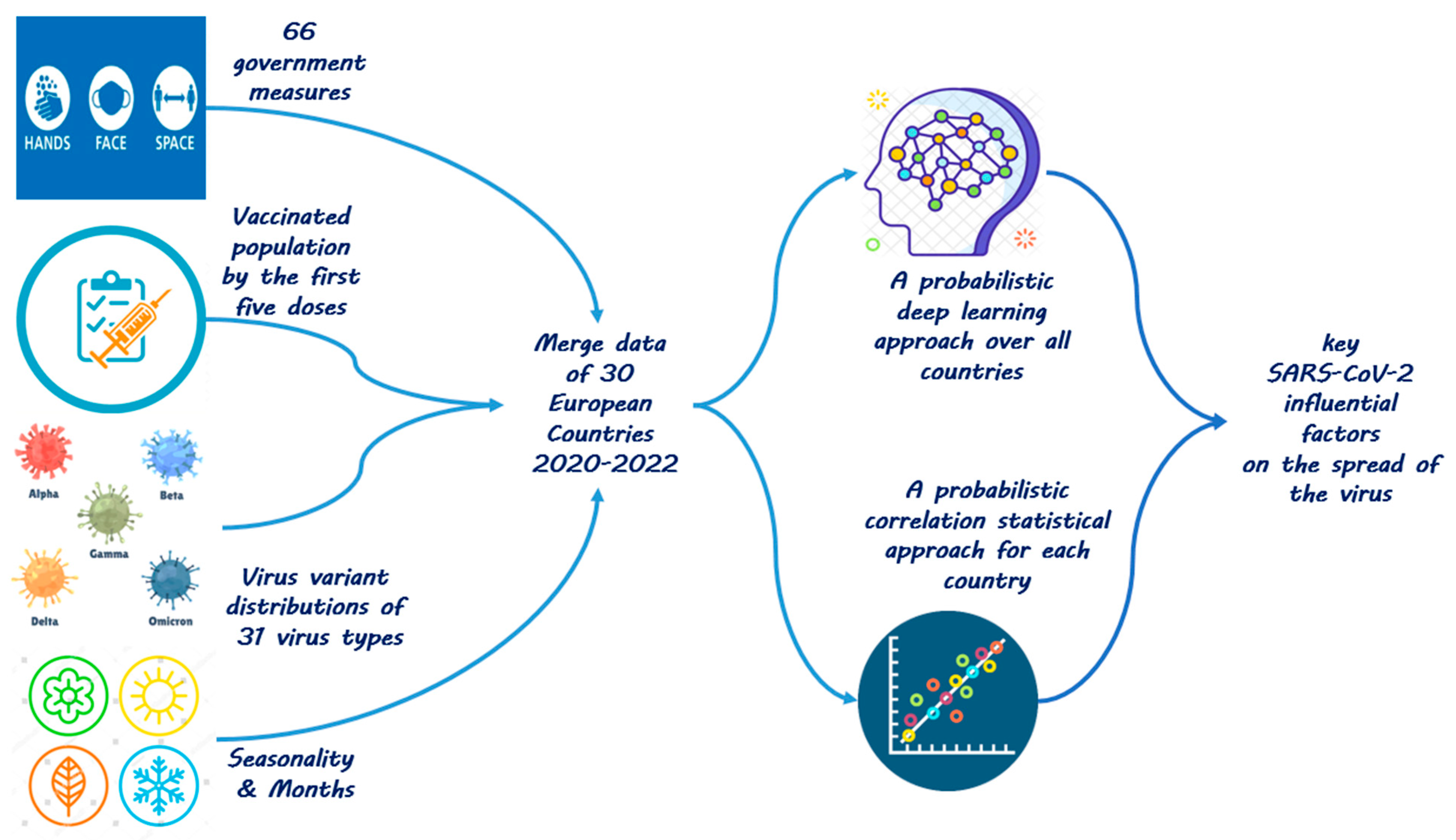
In order to convey a comprehensive understanding of the effects of the European government policies on the spread of SARS-CoV-2, in this study, we combine four datasets with regard to 66 government measures, virus variant distributions (of 31 virus types), and the accumulated percentages of the vaccinated population (by the first five doses) as well as the infection numbers at each day (from early 2020 up to mid-2022) for each of the 30 countries included in this study.
We utilize convolutional deep neural networks (CNNs) [16,17], in particular probabilistic (Bayesian) convolutional deep neural networks (BCNNs) [18,19], together (and in comparison) with Bayesian statistical inference [20,21], as shown in Figure 1.
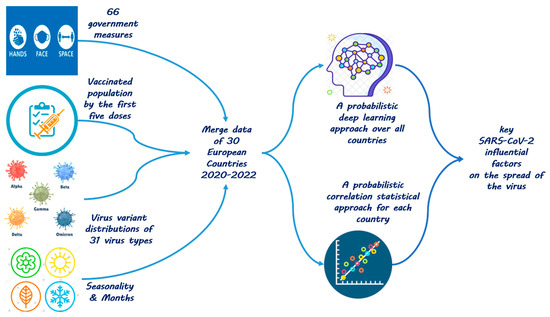
Figure 1.
Approach to analyze the most influential pandemic factors.
We first train a BCNN model, which is capable of predicting the reproduction rate of the virus one month ahead any given day with high accuracy. Based on the trained BCNN model, we infer the importance and the magnitude of the effect of each relevant explanatory factor by applying explainable artificial intelligence (XAI) algorithms. Specifically, the results of two XAI methods are presented in this paper: permutation feature importance (PFI) [22] and partial dependence plot (PDP) [23].
Second, we perform a Bayesian statistical analysis. In the statistical approach, we study two distinct circumstances with regard to each pandemic influential factor in each European country. We look at the distribution of pandemic growth rates in the days where the selected epidemiological factor has been active. Furthermore, we look at the distribution of pandemic growth rates in the days where the selected explanatory variable has not been active in that country. We then compute the probability that the activation of the selected factor—in contrast to the non-activation of it—results in a reduction in the pandemic growth rate.
By applying the first approach, i.e., the convolutional deep model, we aim at utilizing CNNs’ high computational ability [17] to extract the effects of the most critical explanatory variables on the spread of the recent pandemic. By incorporating probabilities in the convolutional deep model in our study, we aim at avoiding over-fitted models through delivering uncertain conclusions [18].
By applying the second approach, i.e., the Bayesian statistical model besides the deep learning model, we try to reexamine the results obtained through the utilized deep learning model with regard to the most critical factors affecting the spread of SARS-CoV-2 within European countries.
The remainder of this paper is as follows: Section 2 provides methodical and scientific foundations for this study with regard to governmental SARS-CoV-2 policies. Section 3 shows how this study’s datasets are extracted, cleaned, and merged into a common data table. Section 4 explains in detail the applied inputs (i.e., the explanatory variables) and the resulting output (the dependent variable) of the deep learning model. It also provides information about the deep learning model with respect to model construction, training, and result interpretation. How a Bayesian statistical analysis is performed is described in Section 5. The results of the deep learning and the statistical inference models are presented in Section 6, while Section 7 is dedicated to the interpretation of these results. Concluding remarks and future research needs are summarized in Section 8.
2. Methodical and Scientific Foundations for This Study
Since the onset of the SARS-CoV-2 pandemic in late 2019, several studies have analyzed important epidemiological factors with respect to the spread of the pandemic in different geographical scopes (e.g., [8,9,10,12,13,14,15,24,25,26,27,28,29]). In this section, we review a set of selected papers based on their relevance to our research subject, especially with regard to the comprehensiveness of the articles’ incorporated explanatory factors as well as the significance of the research’s geographical scope. The key features from the selected articles are summed up in Table 1.

Table 1.
Key features from selected representative set of SARS-CoV-2 epidemiological studies.
The studies comprise a variety of approaches, i.e., statistical analysis [8,9,10,13,14], compartmental methods [12], machine learning techniques [15,24,25,26,28], and deep learning models [27,29].
The included research was conducted in various regions around the globe and conclude with different results. Nader et al. [24] see school closures as an important factor to achieve reductions in infection rates. Li et al. [12] find that mass gathering restrictions and school closings are associated with the largest average reductions in infection rates in large-scale epidemic areas. Ge et al. [8] find that gathering restrictions and facial coverings played a significant role in epidemic mitigation. Liu Y et al. [13] conclude that the rate of masks used in individual prevention does not seem to be related to cumulative mortality or morbidity in European countries. Instead, the mobility index generated by personal behavior might be the more important prevention policy according to these authors. Leech et al. [10] focus on masks mandates as a proxy for mask-wearing effectiveness and conclude that mask wearing reduces the reproduction rate of SARS-CoV-2 by 19 percent. Saleh et al. [27], Zheng et al. [26], Balogh et al. [25], Huy et al. [9], Zhou et al. [15], and Du et al. [29] investigate and approve the significant role of vaccination policy. The significance of the various virus variants beside government interventions has also come into consideration, e.g., in [25]. A complete review of XAI-based epidemiological models of SARS-CoV-2 including the data, methods, and results is conveyed in [30].
In this paper, we proceed with the application of explainable deep learning and statistical methods as in previous studies to identify the importance and magnitude of the most important factors regarding the spread of the recent pandemic. Thereby, our approach in this paper comprises a set of new features. First, by feeding the explanatory factors of the pandemic as 1-dimensional images into a convolutional deep learning model CNN, we extend the literature on using CNN deep networks to epidemiological analysis. CNNs are well-known architectures specifically used for image classification and tasks that consider the processing of spatial dimensions of data [31]. Whereas the usage of CNN-based architecture approaches in the context of clinical studies is practiced [32], the rich potential of performance and interpretability of CNN models is, so far, not substantially exploited in XAI-based epidemiological studies. Second, we treat the dependent variables of our study (i.e., the pandemic reproduction rate in the neural network approach and the pandemic growth rate in the statistical analysis) as uncertain (Bayesian) variables. Incorporating the uncertainty in the model training level is rarely performed in the scope of the SARS-CoV-2 epidemiologic literature. Third, we provide XAI algorithms to understand the significance of a comprehensive set of explanatory features on the spread of the virus in a wide geographical scope consisting of 30 European countries. Fourth, by performing a Bayesian statistical analysis alongside the machine learning approach, we investigate whether the role of each explanatory factor, explained via the deep learning model, can be confirmed with the statistical analysis from a dissimilar perspective.
3. Data
In this paper, we utilize four datasets provided by the European Centre for Disease Prevention and Control (ECDC), which cover 30 European countries:
- Per country per day government measures of NPIs;
- Per country per day virus variant distributions;
- Per country per day per dose new vaccinations;
- Per country per day new reported infections.
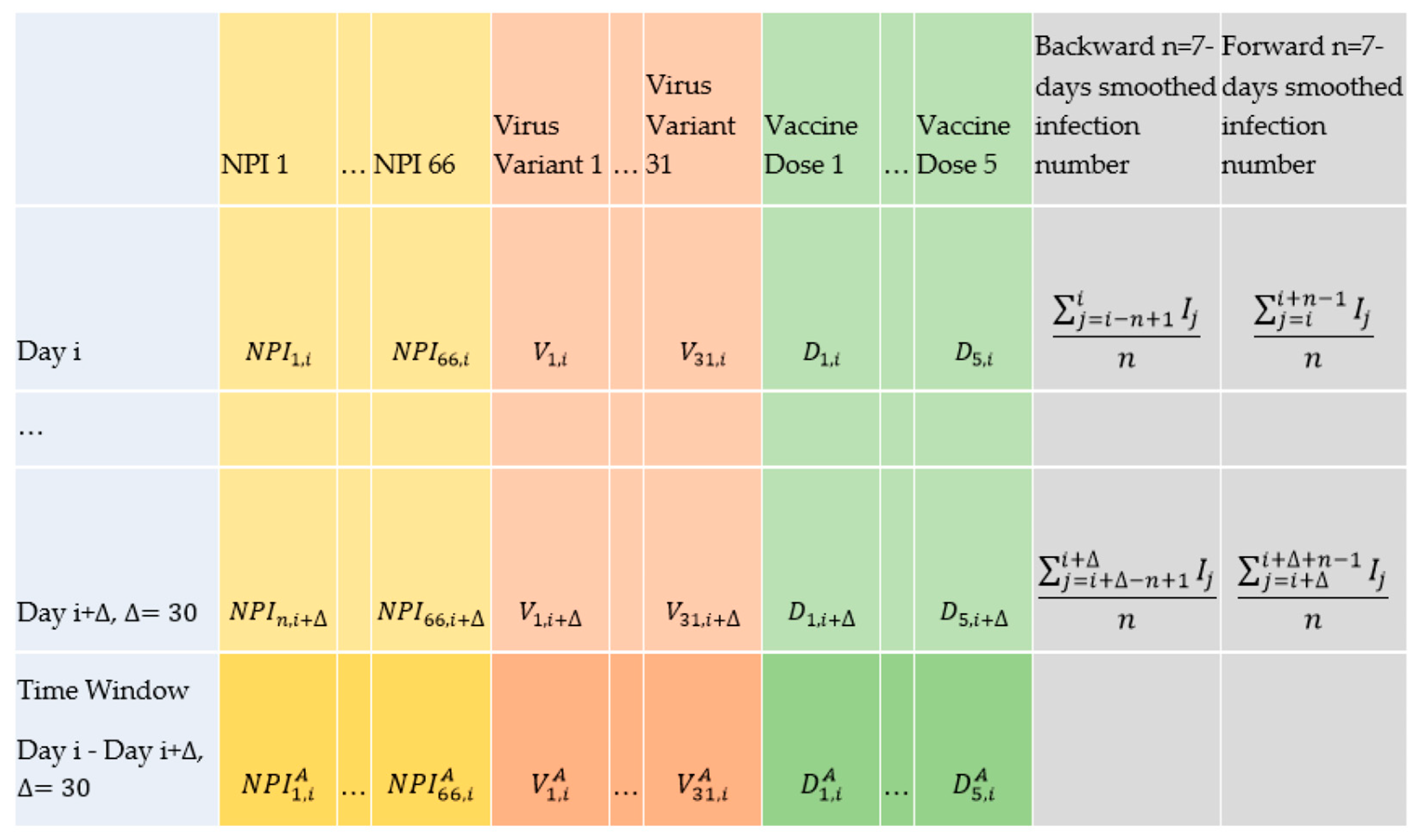
The four datasets are merged into a unique pandas table, referred to as data_encoded. Each row of data_encoded represents each day in the time span between 2020 and mid 2022 for a specific country. Data_encoded consists of 22,420 rows. Each country (from 30 countries) comprises its own block of approximately 750 rows (22,420/30 = 750 days) in data_encoded. The columns of data_encoded comprise 111 columns representing the pandemic explanatory factors as well as 2 columns representing the 7 days’ average backward and 7 days’ average forward number of reported infections at any arbitrary day for each country. These are shown in Table 2 and are explained in the following Section 3.1, Section 3.2, Section 3.3, Section 3.4 and Section 3.5.
Table 2.
The columns of data_encoded representing the pandemic explanatory factors as well as 2 columns representing the 7 days’ average backward and 7 days’ average forward number of reported infections at any arbitrary day for each country.
Data_encoded is appended to the Supplementary Material of this paper.
3.1. Government NPIs
Each of the 66 NPIs applied by governments has a specific column in data_encoded, with a value of 1 if the NPI is active on a day in a country and a value of 0 otherwise. A detailed explanation of these NPIs is presented in [33].
3.2. Vaccination Data
The vaccination data in data_encoded show the accumulated percentage of each of the first five vaccine doses received by the population of each corresponding country in each day. In addition, the pre-vaccination days (where the value for the first dose is equal to 0) and the post-vaccination days (where the value for the first dose is larger than 0) are distinguished for each country’s data in a specific column named vaccination_modus.
3.3. Virus Variants
Each virus variant is presented within a day and in a country by means of the percentage it is sequenced in the corresponding country and day. The sum of percentage values of all sequenced virus variants in a country within each day is equal to 1. There exists a virus variant named ‘Other’ in the list of virus variants, which represents a collection of other, not-labeled virus variants in the data. In addition, the dominant virus variant in each country and each day (as the virus variant with the highest sequenced percentage) owns its own specific column named dominant_virus within data_encoded.
3.4. Country Name and Month Name
The countries’ names (30 categories) and months’ names (12 categories) are considered as categorical variables and hence are hot encoded to distinct sets of 5 digits and 4 digits’ binary formats, respectively. Each digit has its specific column in the data_encoded table.
3.5. Smoothed Infection Numbers
7 days’ average backward and 7 days’ average forward number of the reported infections at any arbitrary day for each country are integrated into data_encoded in two separated corresponding columns. The week-based smoothed numbers are used to compute the dependent variables of our study, i.e., reproduction rates (in Section 4) and growth rates (in Section 5).
4. Bayesian Deep Neural Network Approach
Section 4.1 explains the construction and training process of the applied DNN model. Section 4.2 explains the explainable machine learning algorithms, which are used to elucidate the importance (Section 4.2.1) and the magnitude of the effect (Section 4.2.2) of each relevant influencing input factor on the outcome of the DNN.
4.1. Deep Neural Network Training
The aim of the DNN model in our study is to predict the reproduction of the virus one month ahead of time for each day (as the model output). Thereby, we consider monthly data horizons from each arbitrary day forward as a closed time window (=30 days), to examine the average effects of the explanatory variables within that time window (as the model input).
4.1.1. Model Input
Each input for training the model is constituted by averaging the values of all explanatory variables (Table 2) over the upcoming days from a day i in a country, as depicted in the last row in Figure 2 and explained as follows.
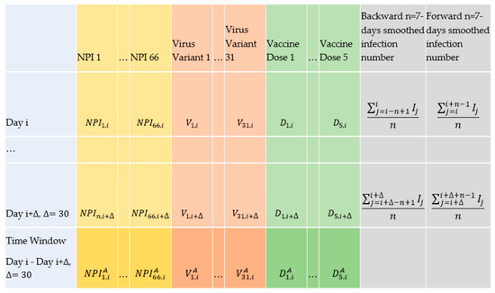
Figure 2.
Representation of the data to form the inputs and outputs in the deep learning and statistical approaches in our study.
For each the average corresponding monthly value is equal to the sum of the NPI values in the days where that NPI has been active within (the days where its value is equal to 1 in data_encoded), divided by the sum of the upcoming days 30 from i.
For each virus variant (), the average corresponding monthly value is equal to the average of that variants’ daily percentages within the upcoming time window from i.
For each vaccination dose (), the average corresponding monthly value is equal to the average of the daily percentages for that vaccination dose within the upcoming time window from i.
For the factor month, if we assume that a specific day i lays within a current month , and the month after is , the average corresponding monthly value is computed as follows:
- ○
- Consider the next days;
- ○
- Weight the hot-encoded and digits (explained in Section 3.4) proportional to the number of the days beginning from i until the end of the current month , i.e., and to the number of the remaining 30 days in the next month i.e., (where );
- ○
- Sum the weighted hot-encoded and digits.
The monthly averaged values of the 111 inputs will then be sorted in a way corresponding to the alphabetical order of variables in Table 2. The sorted set of obtained averaged values forms one training input.
More and more training inputs are generated by iterating over all countries, all days, and all explanatory variables (as explained above) according to the following pseudo-code:
- 1.
- For each country:
- a.
- For each day:
- i.
- Set an empty list;
- ii.
- For each explanatory variable:
- 1.
- Look forward to the next 30 days from each day;
- 2.
- Compute monthly averaged values for that explanatory variable;
- 3.
- Add the computed value in 2 to the list initiated in I;
- iii.
- Consider the completed list of averaged values in step ii.3 as one training input.
For each generated monthly based training input, there exists a monthly based training output described in the next subsection.
4.1.2. Model Output
If the number of observed SARS-CoV-2 positive cases in a country in an arbitrary day j is equal to , and if the average number of observed SARS-CoV-2 positive cases 7 days before the day i, where the window opens, is equal to (see the corresponding cell to the row “day i” and column “backward n-days smoothed infection numbers” in Figure 2), and the average number of observed SARS-CoV-2 positive cases 7 days after the day i + where the window closes is equal to , assuming that, that country’s entire dataset is of length l (see the corresponding cell to the row “day i + ” and column “forward n-days smoothed infection numbers” in Figure 2); then, the monthly based variable , which is analogous to the reproduction rate, is defined according to Equation (5):
While is set to be our study’s predicting object, it is not supposed to represent a kind of causative indicator. is used as a criterion to be a learnable unique output by constructing a deep neural network, which is capable of delivering a thirty-days-forward prognosis regarding the reproduction numbers. One conceivable interpretation of the selected output for our DNN would be that our predictive neural network model is capable of predicting the number of new positive cases 30 days ahead of time by knowing the number of today’s new positive cases and the set of (monthly averaged) input explanatory variables for the upcoming 30 days.
While , being an average monthly based indicator for the spread of the virus, is analogous to the conventional concept of the reproduction rate, we name the reproduction rate of the pandemic throughout our study.
4.1.3. Discretizing Model Output
By defining the output, we tried to train the model via pandemic reproduction rates as a unique continuous output. The code for the regression task is added to the Supplementary Material of this paper. Our attempt to obtain precise predictive results via regression was not effective. Hereby, extending the network by increasing the hidden layers and widening it by increasing the number of nodes did not benefit the precision of the results. This observation could theoretically result from the skewness of the 112 variables (111 input variables and 1 output variable). This happens when most of the values are concentrated in the left or right ends of the x-axis. Nearly all 111 explanatory variables show similar skewness patterns. The distributions of input variables’ values (which can be drawn from month_data_encoded) are either of a right-skewed nature (e.g., B.1.1.7, vaccin_0) or demonstrate highly skewed distributions in both ends of the x-axis (e.g., NonEssentialShopsPartial, month_0). The distribution of the output, i.e., the reproduction values, are highly skewed as well. While about 65% of the reproduction data are between 0 and 2, the maximum output lies around 3500. We also trained the regression task with using logarithmic transformation of the output data; however, this did not improve the model precision. The inefficiency of the regression model is hypothesized by us to be due to the fact that, in the transformation approach, not only the skewness of the output but also the skewness of the inputs matters. This is because both input and output skewness can affect the regression intercept as well as the coefficients associated with the model.
This idea shifted us towards defining the problem as an image classification task analogous to the MNIST classification problem (which is a large database of handwritten digits for training image recognition tasks [34]). Thereby, we aim at the recognition of pandemic 1-D pictures (inputs) by means of classification labels (outputs). Hence, we translate s to 100 bins (ranging from 0 to 99). The bins contribute to presenting the output side in a balanced way, because each bin represents equal percentile amounts of s in itself. In that way, we did not miss that much preciseness. Each bin’s range () is sufficiently fine grained to reflect the original values precisely enough. This can be evidenced by the fact that the median of the difference of values laying in two subsequent bins is 0.027 while the median value of values is 1.175. After extracting the model’s categorical predictions in the form of reproduction percentiles, when presenting our results, we translate them again to the original values, in which we compute yet again the mean value of the minimum threshold (and the maximum threshold of the corresponding bin, i.e., .
4.1.4. Constructing the Bayesian Deep Learning Model
Each training input and training output is generated based on computing the monthly averaged values of data_encoded as described in previous subsections. The month-based averaged values are stored in a new table named month_data_encoded (attached to the Supplementary Material of this paper) to be used for model training. The generated training inputs and outputs (stored in month_data_encoded) are fed into a convolutional neural network (CNN) model. CNNs are deep learning approaches which are typically used to solve image classification tasks [17,35]. In this paper, however, we use CNNs in the epidemiological context. Our reason for choosing CNNs is their ability to detect combined features in image recognition tasks. CNNs perform convolution operations in the upstream layers of the network, where the filters extract the most critical features to generate a feature map. The extracted features can not only be of spatial or temporal nature but also be used to recognize a range of government policies. For example, the combined effects of government policies such as ‘ClosDaycare’, ‘ClosDaycarePartial’, ‘ClosHigh’, ‘ClosHighPartial’, ‘ClosPrim’, ‘ClosPrimPartial’, ‘ClosPubAny’, ‘ClosPubAnyPartial’, ‘ClosSec’, ‘ClosSecPartial’, etc., are presented as neighbor image pixels and hence will be better considered in CNNs.
CNNs are not fit by default to incorporate the factor uncertainty, which is crucial when dealing with relatively small or uncertain data areas. In contrast to CNNs, the Bayesian neural networks (BNNs) approach [18,19] delivers a robust method in terms of offering uncertainty. BNNs can easily learn from small and uncertain datasets. Integration of BNNs and CNNs means a probabilistic interpretation of the deep learning CNN model by inferring distributions over the models’ weights and offering distributions over the models’ outputs, i.e., BCNN. BCNN models are less prone to get into overfitting traps and can cope with scare data through delivering uncertain outcomes.
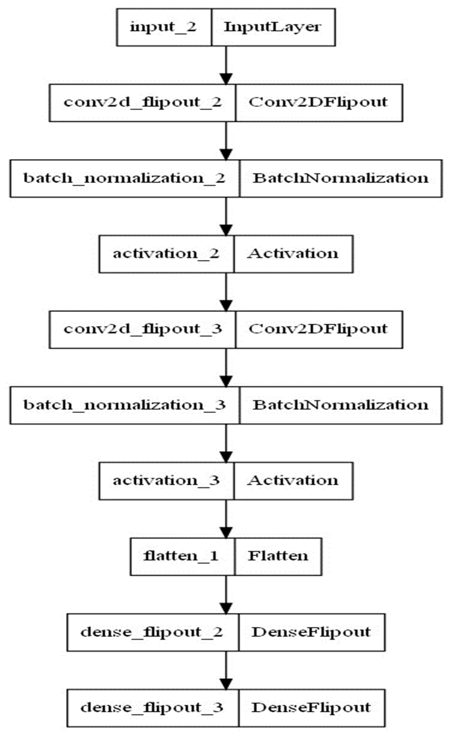
Technically, we treated the input and output pandemic data like we treat the above-mentioned MNIST data. Each MNIST input data point contains the pixel data for the handwritten digit in the form of an image with dimensions (28, 28). We flatten the data to obtain a (1, 111) image array. We use the tensor flow probability (TFP) package to combine probabilistic models and convolutional deep learning. Thereby, batch normalizations are used as supplement layers after each convolution layer to alleviate the risk of overfitting by normalizing the input values of the following layers [36]. Furthermore, the inference is guaranteed by using the flip out estimator [37], which performs a Monte Carlo approximation of the distribution integrating over the weights and biases. The loss function consists of Kullback–Leibler divergence and soft-max cross entropy to quantify the difference between the predicted outcomes’ probability distribution from the real outcomes’ probability distribution [38]. The number of kernels, output units and dropping rate are chosen by experimenting with the model and without utilizing parameter tuning algorithms. Furthermore, the Adam optimizer and a learning rate value equal to 0.001 are used. The model architecture is summarized in Figure 3 and Table 3.
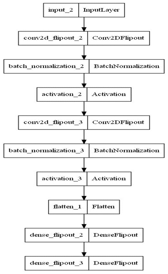
Figure 3.
Architecture of the BCNN model.
Table 3.
Summary of the BCNN model.
4.2. Deep Neural Network Explanation
We employ two explainable ML algorithms introduced in the following two subsections to understand the significance and magnitude of each explanatory factor of our study.
4.2.1. PFI
In order to assess the importance of each input feature (explanatory variable) on the predicted reproduction rate of the virus in the DNN model, we apply the permutation feature importance PFI algorithm. The algorithm works as is shown in the following pseudo-code based on [22]:
- Input: Trained model , feature matrix X, target vector y, error measure L(y,)
- 1.
- Estimate the original model error eorig = L(y,(X)) (e.g., mean squared error)
- 2.
- For each feature j∈{1,…,p} do:
- 1.1.1.
- Generate feature matrix Xperm by permuting feature j in the data X. This breaks the association between feature j and true outcome y.
- 1.1.2.
- Estimate error eperm = L(Y,(Xperm)) based on the predictions of the permuted data.
- 1.1.3.
- Calculate permutation feature importance as quotient FIj = eperm/eorig or difference FIj = eperm−eorig
- 3.
- Sort features by descending FI.
Thereby, one can estimate the significance of each input feature (explanatory variable) by calculating the increase in the model’s initial prediction error (step 1) after permuting (shuffling) that feature within all rows of a selected set of data (hereby, randomly selected 25% of the entire dataset). Due to the incorporated uncertainty in the predicted outputs of the BCNN model, the sub-step 1.1.2 of the above algorithm is repeated 100 times, resulting in the estimated error being equal to the mean value of the 100 resulted root mean squared errors.
4.2.2. PDP
To shed light on the effect each relevant input feature might have on the predicted outcome of the DNN model, we apply the partial dependence plot PDP algorithm [23]. By means of the PDP, we aim at understanding two distinct counterfactual scenarios, in which one selected explanatory factor could turn out to be 1 (representing its activation within all days in the data of a country) or zero (representing its inactivation within all days in the data of a country). We perform this procedure in a country-wise manner over the entire existing rows of each country’s data. For each explanatory factor and each country, we compute the average predicted outcome via counterfactual inactivation of that factor in the country’s entire dataset, which is assumed to be of length l:
We then compute the average predicted outcome via counterfactual activation of that feature in the country’s entire dataset.
We then subtract the activation-related outcome from the inactivation-related outcome.
The can be interpreted as average gains expressed in terms of the difference in reproduction values when activating each feature in each of the thirty countries, for which data are available:
- A positive means that the average reproduction rate is predicted to be smaller under the full activation scenario of that factor on all days of the pandemic time in the corresponding country;
- A negative indicates greater predicted reproduction numbers under full activation scenario of that factor on all days of the pandemic time span in the corresponding country.
Note that, similar to the procedure conducted in Section 4.2.1, due to the incorporated uncertainty in the predicted outputs of the BCNN model, the prediction task for each row of data is accomplished through 100 repetitions.
5. Bayesian Statistical Approach
In this section, we perform a statistical inference analysis for each explanatory factor within each of the 30 European countries. Thereby, we use the information regarding the 7 days’ average backward and 7 days’ average forward number of the reported infections at any arbitrary day for each country from data_encoded.
If the average number of observed SARS-CoV-2 positive cases 7 days before any day i is equal to (see the corresponding cell to the row “day i” and column “backward n-days smoothed infection numbers” in Figure 2) and the average number of observed SARS-CoV-2 positive cases 7 days after the day i is equal to , n = 7 (see the corresponding cell to the row “day i” and column “forward n-days smoothed infection numbers” in Figure 2), then, the daily based variable is defined according to Equation (9):
represents a kind of symmetric predictive criteria to indicate the change in the spread of the virus between the 7 days’ average backward and 7 days’ average forward values for any arbitrary day i. Hence, is the daily relative growth rate of the pandemic. For each influencing input factor, the distribution of pandemic growth rates in the days where the selected explanatory factor has been active is compared with the distribution of the pandemic growth rates in the days where the selected explanatory variable has not been active.
5.1. Bayesian Statistical Model
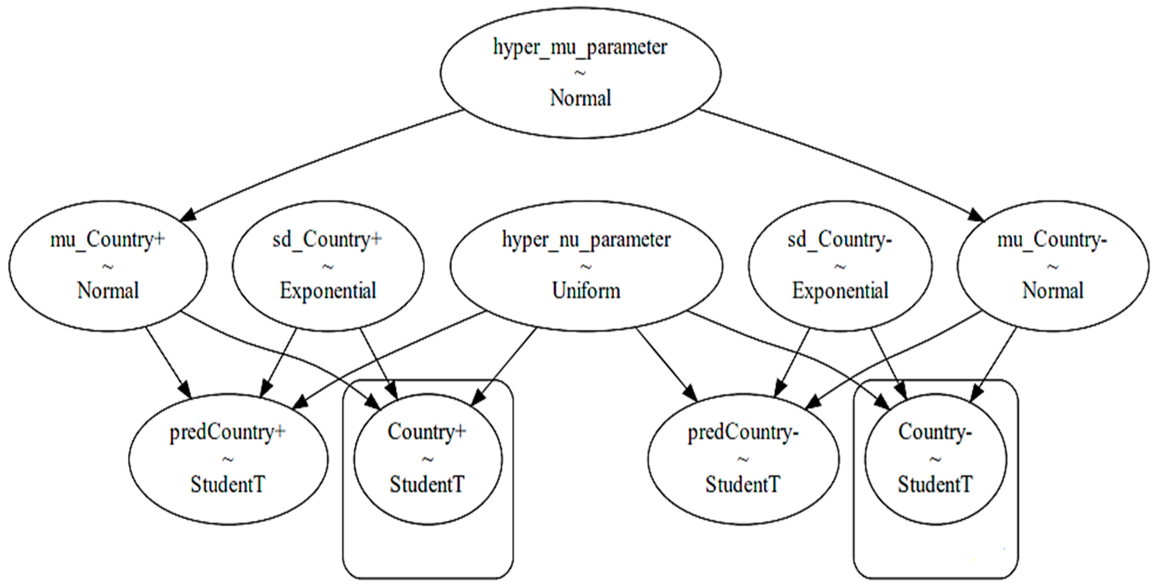
To obtain the posterior probabilities with regard to the presence and non-presence of a selected explanatory factor in each country, we took each country’s data separately and analyzed each explanatory factor within the selected country’s data by means of a hierarchical Bayesian model [20,21]. A hierarchical Bayesian model considers a hyper parameter at the top level of its analysis, as well as specific parameters in its lower level. The top hierarchical level takes the overall distribution of growth rates in a certain country into account regardless of the condition whether the certain explanatory factor has been active or not. The lower level takes the situation-specific developments into account, i.e., whether the selected epidemiological factor is implemented or not. The model used in this paper is illustrated in Figure 4.
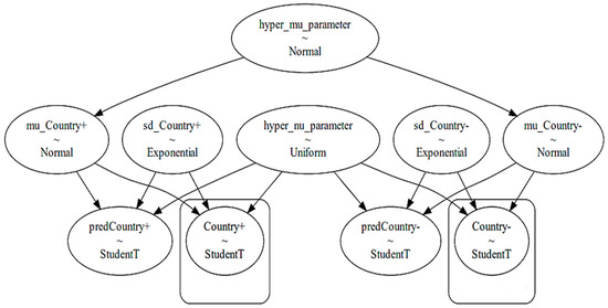
Figure 4.
The hierarchical Bayesian model for analyzing a distinct explanatory variable in a distinct country (variables in boxes are observed variables).
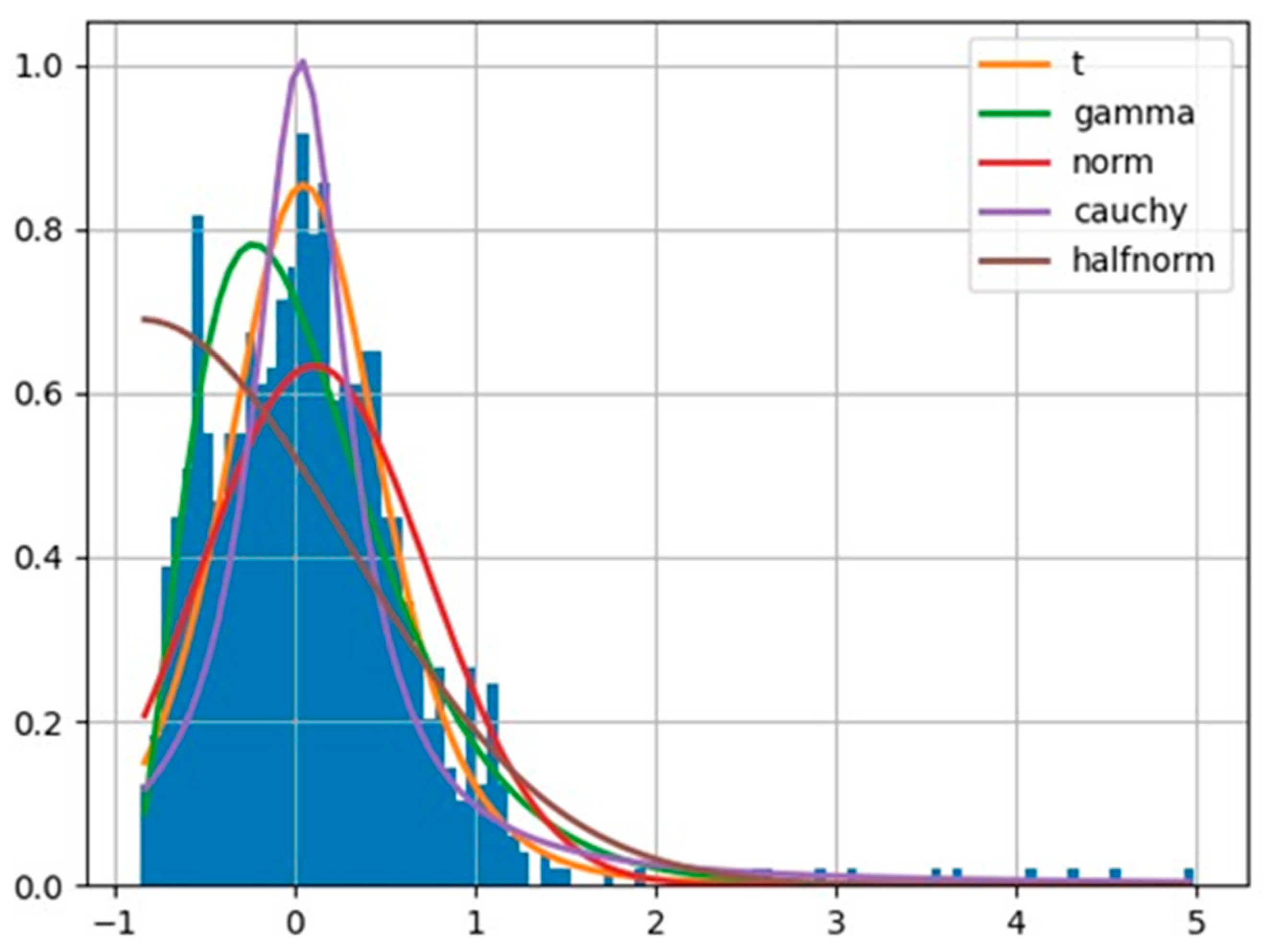
The top level of the model in Figure 4 depicts the hyper mu parameter, which is a normal distribution function consisting of a mean and a standard deviation for a distinct country from the studied countries. The mean and standard deviation are derived by us through considering all observed data within a selected country. The left-hand side of the model (consisting of variables with positive sign at the end) devotes itself to the effect of activation of a certain explanatory factor on the epidemic growth rates. The right-hand side of the model (consisting of variables with negative sign at the end) devotes itself to the effect of non-activation of the selected explanatory factor on the epidemic growth rates. The lower level of the model uses the Student’s t-distribution to infer posterior predictive values. The reason of choosing a Student’s t-distribution is its fitness to the shape of the in the studied countries. Thereby, we used the fitter package (https://github.com/cokelaer/fitter, accessed on 18 June 2024) in python to explore aggregate and individual data across the studied countries. The histogram of the overall s numbers with the example of Germany during the pandemic is demonstrated in Figure 5.
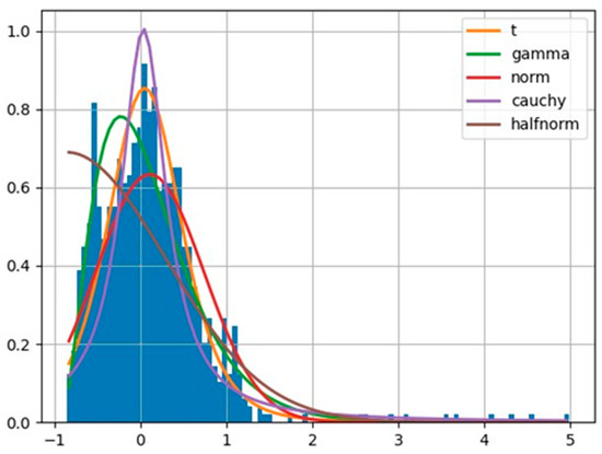
Figure 5.
Student’s t-distribution fits optimally to describe the likelihood function of growth rate values in Germany.
The hyper parameter nu is the degree of freedom part of the subsequent Student’s t-distribution, which usually ranges from 0 to 30 and becomes shared between the left-hand side and the right-hand side of the model. The presence of the sd_Country parameters specified in both the right-hand side and left-hand side of the model figure provides a weekly informative prior which permits the lower level of the model to sample its parameters (either corresponding to the activation of a factor on the left-hand side or corresponding to the non-activation of the selected explanatory factor in the right-hand side) without bias. While a basically normal distribution provides a reasonable prior for the mean parameter, the exponential distributions provide reasonable priors for the standard deviation, i.e., for the distribution of the abovementioned sd_Country terms [21].
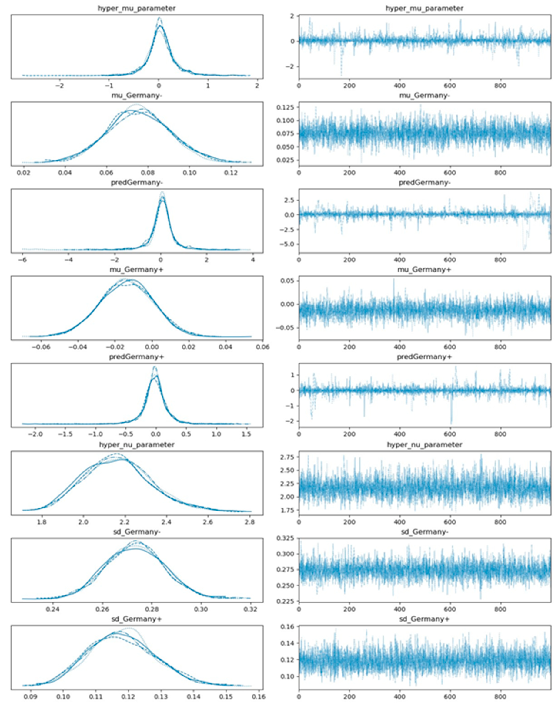
Obtaining posterior distributions with regard to the presence and non-presence of a selected factor is often analytically intractable. The sampling procedure of the posterior distributions are accomplished via using a No-U-turn sampler (NUTS) implemented in the probabilistic programming package for python PyMC3. The results of the posterior sampling draws get stored in a PyMC3 data object called trace. The values of a trace not only represent the obtained posterior values but also can reveal the reliability of the parameter space exploration via the employed sampling algorithm. The model trace convergence is evaluated by means of the Gelman-Rubin R_hat statistic [39]. R_hat values deviating from one indicate that trace values move wildly or get stuck and that sampling failed to cover the parameter space effectively. Hence, in practice, we are looking for R_hat values close to one. The resulting trace plots regarding the predicted distributions of s in the case of implementing gym and sport center closures (predGermany+) versus non-implementation of the gym and sport center closures (predGermany-) in Germany are shown in Figure 6.
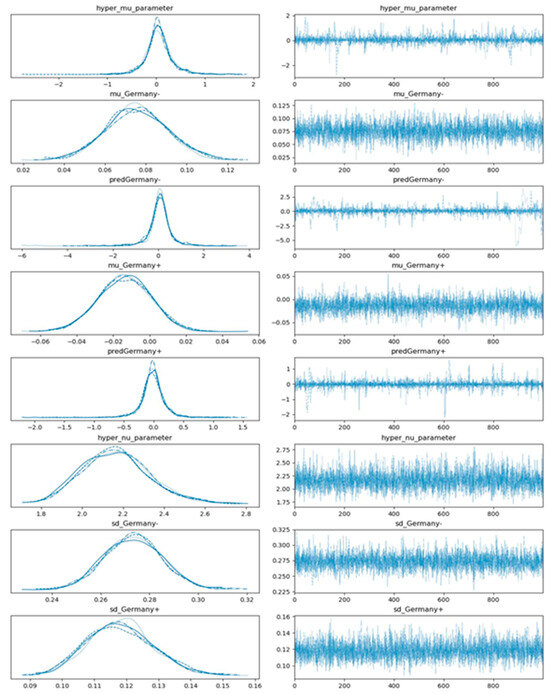
Figure 6.
Estimated plot distributions (left-hand side panels) and the corresponding sampled values (right-hand side panels) via multi-process sampling with regard to the effect of gym and sport center closings in Germany based on the hierarchical model depicted in Figure 4. Note that 4 subplots in each left-hand side panel comprise 4 different chains, each of them comprising 1000 draws (solid line: chain 1, dotted line: chain 2, dashed line: chain 3, and dot-dashed line: chain 4).
5.2. Computing the Term Efficiency by Comparing Distribution Samples
In this subsection, we assume we have obtained the posterior distributions of the pandemic growth rates in the days where a selected explanatory variable has been active, as well as the posterior distributions of the pandemic growth rates in the days where the selected explanatory variable has not been active.
We define the efficiency of a factor to figure out the probability that, in an arbitrary chosen day, the presence (activation, “+”) of a factor grants less value to the growth rate of the virus in comparison to the absence (non-activation, “−”) of that factor. We do the comparison stochastically by sampling 1000 random draws from both positive-signed and negative-signed distributions. Moreover, 1000 random draws from the positive-signed posterior distribution will generate a list L of growth rates named , which is of length 1000. Likewise, 1000 random draws from the negative-signed posterior distribution will generate a list of growth rates named , which is of length 1000. The efficiency ratio (Equation (10)) results from the iterative comparison of each positional element l (from 0 to 1000-1) of the above-mentioned two generated lists, setting the comparison term equal to 1 if it is true and 0 if false, and calculating the averaged compared values:
To offset the stochastic nature of computing via random drawn growth rates, we repeat computing 1000 times and look at the distribution.
5.3. Exemplary Computation of the Efficiency Term
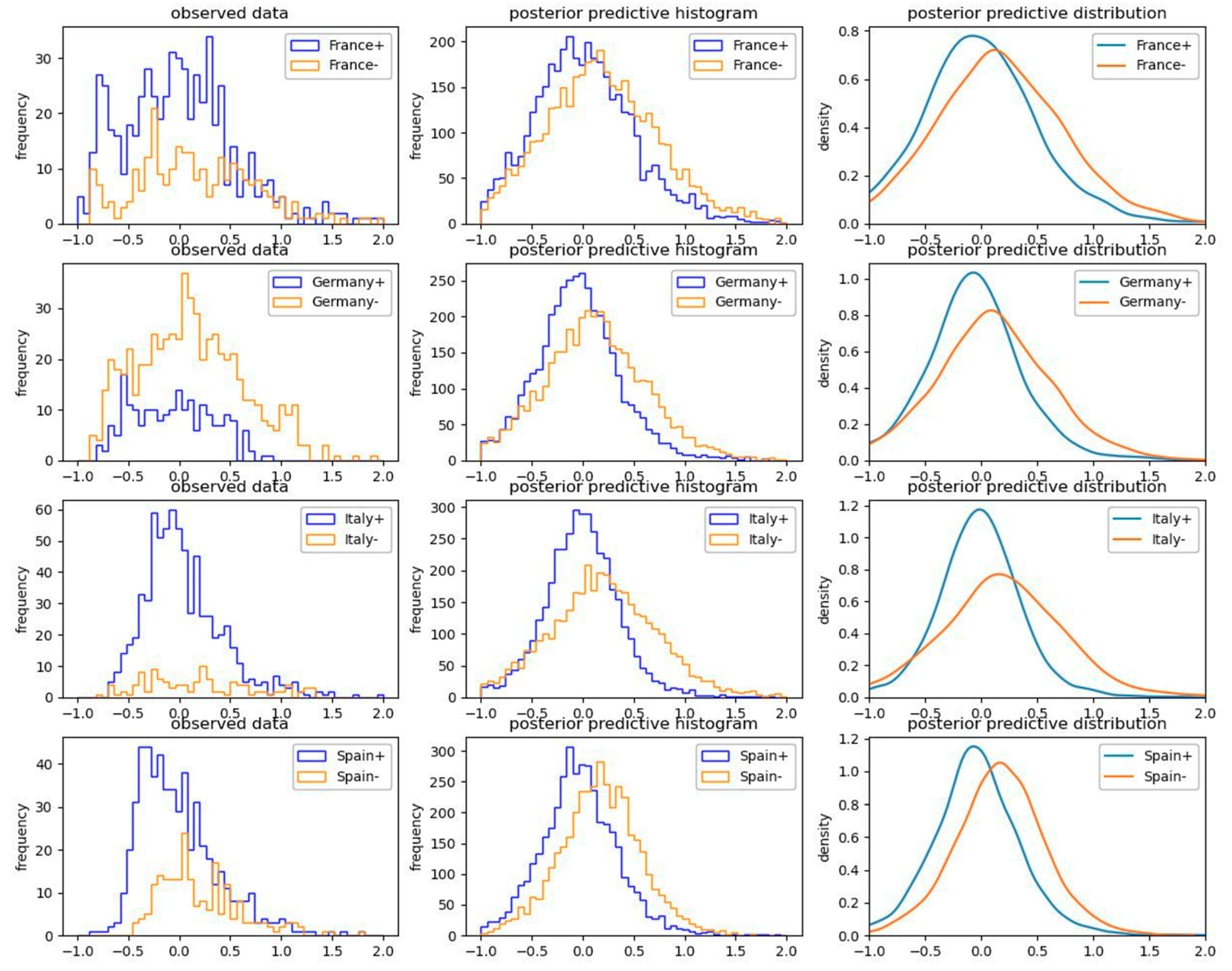
Figure 7 and Figure 8 illuminate the inference procedure from the observed empirical data up to computing the efficiency terms by means of the example of “closure of gyms and sport centers” in the four most populated European countries (France, Germany, Italy, and Spain).
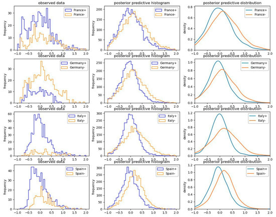
Figure 7.
Posterior predictive results regarding activation (“+” positive sign) versus non-activation (“−” negative sign) of the explanatory factor of “closure of gyms and sport centers” in the four most populated European countries.
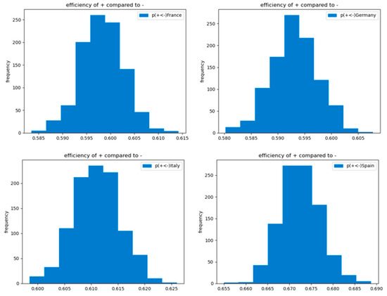
Figure 8.
Efficiency of the implementation of the selected NPI (gyms and sport centers closures) in comparison to non-implementation of it within the selected subset of countries.
Each blue line at the left-hand side of Figure 7 displays the empirically observed growth rate of the pandemic in the days when the selected factor (closure of gyms and sport centers) has been active in each selected country. Each orange line on the left-hand side of Figure 7 displays the growth rate of the pandemic in the days when the selected factor has not been active in each selected country. The posterior predictive probabilities in the middle and the right-hand side of Figure 7 are driven by sampling posteriors using NUTS.
The obtained posterior probability distributions of activation versus non-activation of the selected explanatory factor in Figure 7 are compared in line with the logic explained in Section 5.2 and expressed in Equation (10). The histogram of the obtained 1000 computed efficiencies is presented in Figure 8.
6. Results
6.1. Verifying the Accuracy of the Bayesian Deep Learning Model
The BCNN model is trained with 1000 epochs over 80% of the data, which covers 21,549 rows of month_data_encoded. The training code (to replicate the training process) and the saved model (to regenerate the model predictions) as well as training and evaluation losses and training and evaluation root mean square errors are appended to the Supplementary Material of this paper. Figure 9 reveals the preciseness of the predicted (month-based) reproduction rate percentiles of the model for a hold out set comprising 20% random split test data as well as for the training and evaluation datasets.
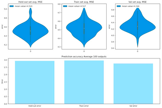
Figure 9.
Model metrics over hold out, training, and evaluation datasets.
The violin plots of the upper panels in Figure 9 demonstrate the distribution of 100 resulting root mean square errors, when the saved model is prompted 100 times to predict reproduction rate percentiles. As one can see, the estimated error between the predicted reproduction values and the actual values is less than 5% in all 3 sets. The lower panel in Figure 9 demonstrates the root mean squared errors, when the saved model is required to predict reproduction rate percentiles 100 times, and the predicted value for each input is calculated by averaging the entire 100 predicted values for that input and then compared to the actual one. The result indicates that the estimated errors are less than 3% for each of the hold out, training, and evaluation sets, if we utilize the BCNN model’s average predicted outputs.
6.2. Verifying the Accuracy of the Bayesian Statistical Analysis
The detailed results regarding the summary of efficiencies and the detailed statistics corresponding to each factor in each of the 30 countries are attached to the Supplementary Material of this paper. The r-hat statistic for all the obtained results is approximately equal to 1.0 for all parameters. This indicates no problems during sampling.
6.3. Bayesian Deep Learning Results
In this subsection, we present the corresponding results of the Bayesian deep learning approach. The resulting PFI importance of variables is presented in Table 4. The explanatory factors with higher values in Table 4 can be interpreted as the ones with higher importance. In contrast, the explanatory factors with lower values in Table 4 can be interpreted as ones with the lowest importance. The Base line, which represents the zero-importance level, is located between some not frequently observed virus variants, i.e., BA.2+L452X and BA.4/BA.5.
Table 4.
Importance of explanatory variables with regard to their impact on pandemic reproduction based on PFI.
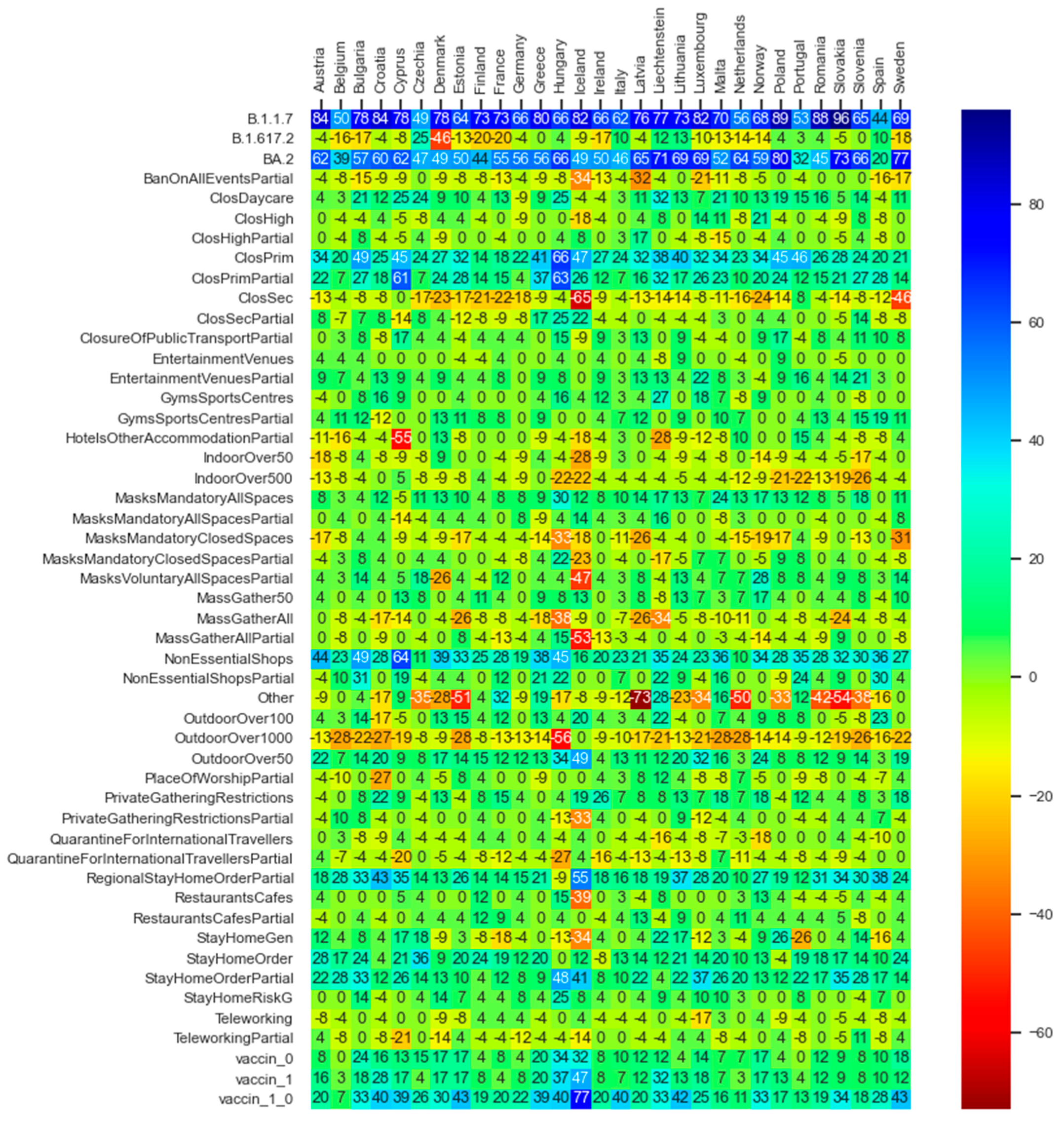
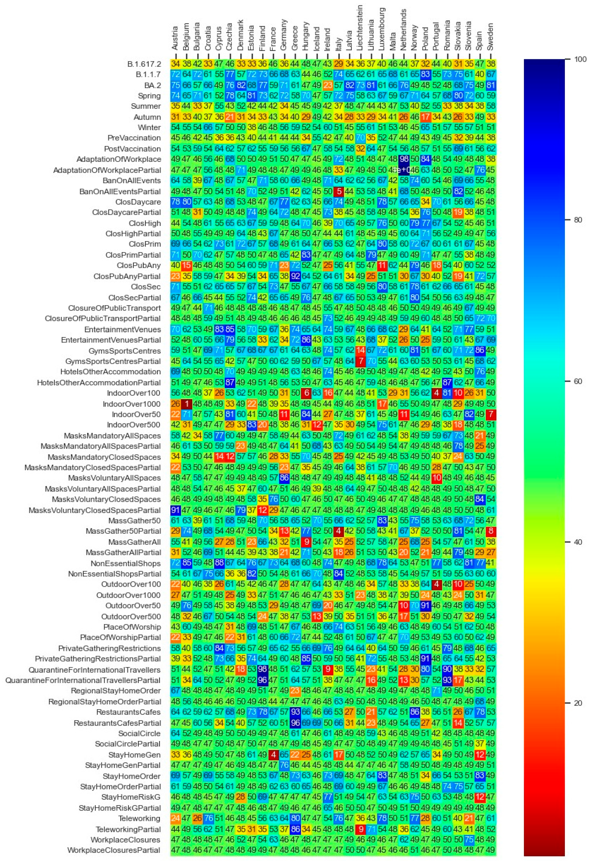
The depicted values in the heat map diagram in Figure 10 express average gains measured in terms of alteration of reproduction values to contain the pandemic growth if one feature is active in comparison with the circumstance of that feature being non-active in line with the PDP notion.
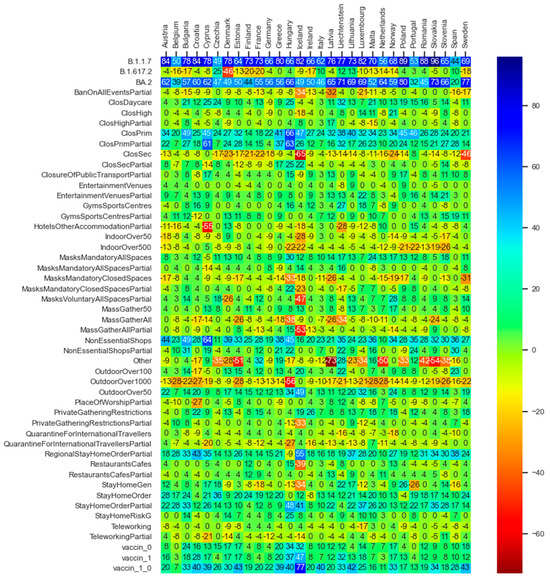
Figure 10.
Average gains expressed in terms of difference in reproduction values when activating each feature in each of the thirty countries for which data are available.
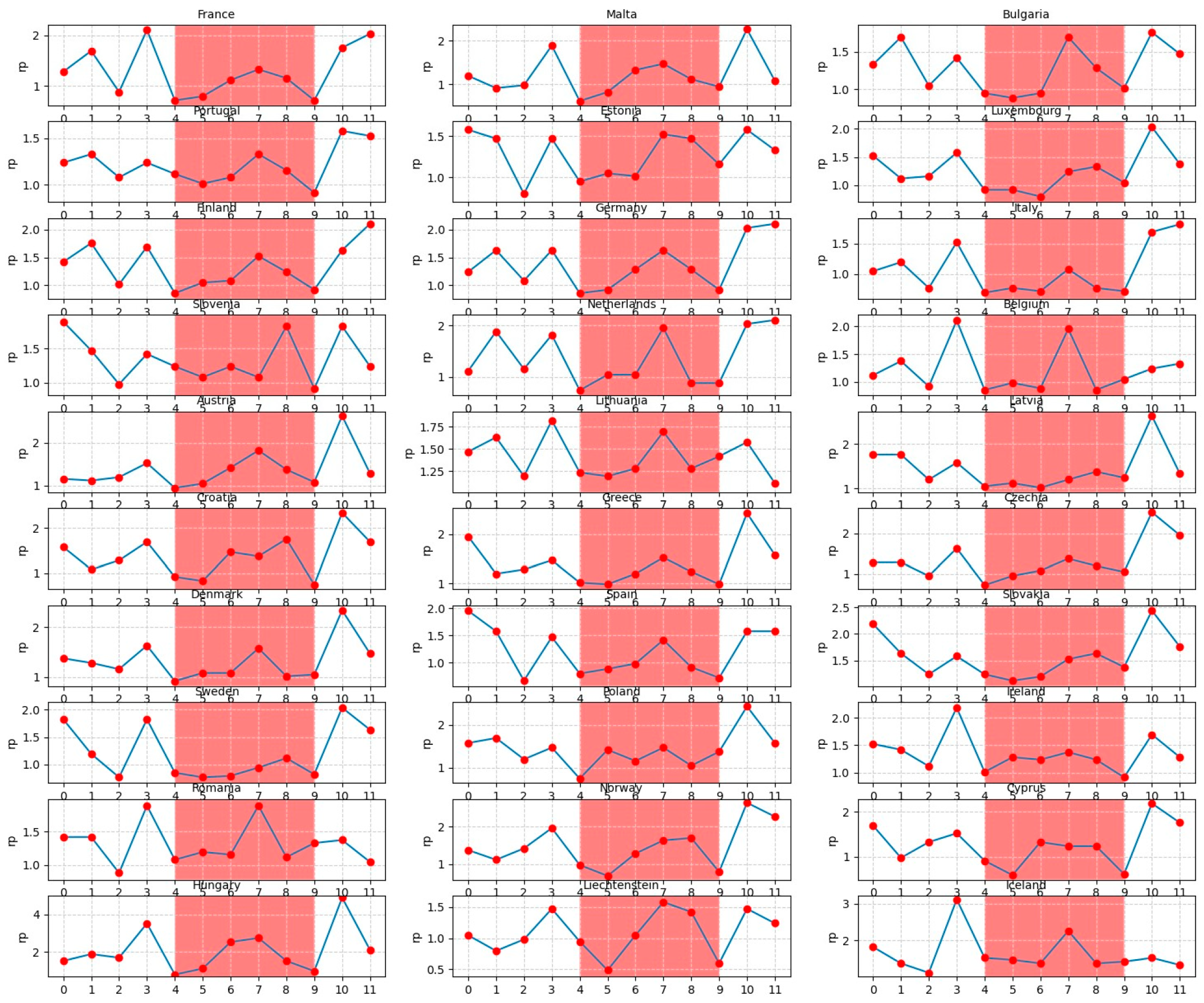
Figure 11 illustrates the month-wise computed PDPs covering the counterfactual scenarios of all months of the year being set each time to a specific month ranging from 0 (December) to 11 (November). In Figure 11, a specific period of the year for each country between the month 4 (April) and the month 9 (September) is highlighted in light-red as it demonstrates the season belonging relatively to the warmer times within the year.
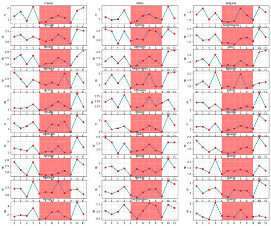
Figure 11.
Monthly predicted average reproduction values for European countries within a time span of 12 months.
6.4. Bayesian Statistics Results
In this subsection, we present the corresponding results of the Bayesian statistics approach. Figure 12 demonstrates the average values corresponding to each explanatory factor’s efficiencies from the statistical inference analysis. The max and min values of the obtained values differ in the range of less than 2 percent from the depicted mean values in Figure 12.
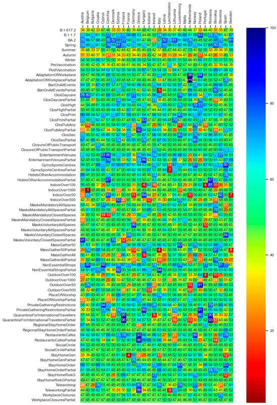
Figure 12.
Summary of each explanatory factors’ average efficiency in percentage values.
In order to summarize the statistical inference for each explanatory variable (depicted in Figure 12), the average of the efficiencies over the entire 30 countries is computed and illustrated in Table 5. In Table 5, explanatory variables with higher than 50 percent efficiency values (e.g., the season Spring and the alpha variant) can be interpreted as effective factors with regard to pandemic containment. In contrast, explanatory variables (e.g., the season Autumn or the omicron variant) with under 50 percent efficiency values can be interpreted as effective factors with regard to pandemic growth.
Table 5.
Sorted average efficiencies of the pandemic factors over all studied countries.
7. Interpretation of Deep Learning and Statistical Findings
The analysis of the importance of explanatory factors (Table 4) indicates that the factor country is at the top level of epidemiological factors in the predictions of the model. The high importance of the factor country is caused by the construction of the DNN model, since this factor is not averaged over different countries, which would make no sense for this factor. Each country is a unique key for the data solely corresponding to that country. It remained in its place during the training of the model. However, seeing the factor month—which is taken into account during the training procedure of the BCNN model—at the top of all other explanatory features is remarkable.
Consequently, we conclude that the months and seasons have been much more influential on the dynamics of the SARS-CoV-2 pandemic in comparison with the governments NPIs and vaccination policies as well as the emergence of virus mutants. The evidence from the counterfactual PDP exploration of seasonal effects (Figure 11) is twofold: First, the overall reproduction rates in the white area are significantly higher than those within the light-red area. Second, in most of the countries, there is a peak in the virus spread around month 7 (July). The existing literature explores the role of seasonal trends. Merow and Urban [40] develop statistical models that predict the maximum potential of COVID-19 worldwide and throughout the year. The authors predict that COVID-19 will decrease temporarily during summer, rebound by autumn, and peak next winter. In a more recent study, Wiemken et al. [41] use time-series decomposition to extract the annual seasonal component of COVID-19 cases, hospitalization, and mortality rates from March 2020 through December 2022 for the United States and Europe. The authors identify seasonal spikes in COVID-19 from approximately November through April for all outcomes and in all countries. These results are indeed, to a large extent, in line with the predictions of our deep learning model. In addition, the results of the statistical inference analysis (Figure 12 and Table 5) regarding the seasonality effects support that large probable growth rates of the virus are visible in the Autumn season (September, October, and November) and the smallest pandemic growth is predicted to be in the Spring season (March, April, and May). The statistical inferences show that the gained efficiencies in Winter (December, January, and February) are higher than the efficiencies of Summer (June, July, and August). Note that as the statistical inference analysis uses the data of each country separately, the months are summarized into the seasons so as to increase the number of prior observations per season in each country. Returning to the spike in July in the DNN model (Figure 11), the frequently observed peak in summer in most of the countries (e.g., Hungary in July, Liechtenstein in July–August, Belgium in July, Bulgaria in July, Estonia in July–August, Netherlands in July, Lithuania in July, etc.) can be hypothesized to be a result of the surge in the infection cases through less-restricted public mobility during summer vacation.
The deep neural network model as well as the statistical inferences both provide evidence that the three well-known variants of the virus (i.e., B.1.1.7—Coronavirus Alpha variant, B.1.617.2—Coronavirus Delta variant, and BA.2—Coronavirus Omicron variant) have seemingly played a significant role in driving the dynamics of the pandemic, i.e., higher influence on the virus spread than the governments’ NPIs and vaccination programs. The PDP analysis of the DNN model (Figure 10) also evidences that, in the light of the assumption regarding the counterfactual scenario of the pandemic getting stuck by the mere presence of B.1.1.7 (Coronavirus Alpha variant), a considerable reproduction rate reduction of up to around 90 percent could have been achieved. The rows of Figure 10 regarding the B.1.617.2 (Coronavirus Delta variant) and BA.2 (Coronavirus Omicron variant) variants reveal to what extent the counterfactual predominance of the Omicron variant could have been beneficial in terms of amelioration of the virus spread and how the hypothetical extension of the delta variant could be harmful. Note that a row named ‘Other’ exists, which indicates the potential harmful effect of other not-labeled virus variants in the dataset; if such virus variants could prevail, the pandemic scene might have gone beyond the destructive role of the delta variant. The same inferences regarding the role of the major virus variants can be obtained through the statistical inference analysis (see Figure 12 and Table 5).
While the outcomes disclose the role of the explanatory factors within each country separately, the overall results indicate that, generally, the government policies might have played a subordinated role compared to the seasonality and virus variants.
Figure 10 and Figure 12 illustrate that, in the majority of countries, the efficiency term (Section 5.2) of the post vaccination period is relatively higher than the pre-vaccination period. The factor vaccine_0_1 in Figure 10, which expresses the counterfactual scenario of the whole population being vaccinated with the first and the second dose within all phases of the pandemic, reveal the relatively high effectiveness of the vaccination policy to constrain the spread of the virus.
Beyond the month and season factors of the NPIs, closing the primary schools, general and regional lockdowns, and non-essential shop closures were significant in reducing the pandemic reproduction, both in the DNN model and the statistical inference model.
While in the literature the effects of government mask mandates are to some extent inconsistent [10], the partially inconsistent representation of the mask mandates in closed spaces in Figure 10 and Figure 12, and Table 5 need to be further researched. The explanatory factor MasksMandatoryAllSpaces encompassing the protective mask usage in all public spaces on a mandatory basis (enforced by law) is predicted through the DNN model to have positive influence to combat the pandemic. However, it is peculiar that the factor MasksMandatoryClosedSpaces representing protective mask use in closed public spaces/transport on mandatory basis (enforced by law) is contributing to increase infection rates in most of the countries.
This requires further research on the role of mask mandates to control the pandemic. Kai et al. [42] put forward some hypothesis that enforcing masks works if and only when the entire or at least a substantial mass of the society becomes committed to it. And it becomes significantly inefficient if mask wearing is prescribed or obeyed partially [42] or if the observed levels of mask wearing in closed spaces are critical [10]. Barceló and Sheen [43] raise the question of the effectiveness of mask mandates in regions where commitment to face masks lacks a cultural background [43]. Despite the conjectures, examining the predicted non-efficiency of mask mandates in closed spaces, despite the high efficiency of the all spaces mask mandates, as shown in Figure 10 and Figure 12, and Table 5, might not be explained completely based on the above hypothesis nor within our analysis. It requires further research.
8. Conclusions
In this paper, we applied a deep Bayesian convolutional neural network and a Bayesian inference statistical model to analyze the SARS-CoV-2 government policies across thirty European countries. The data explored include 66 government measures, virus variant distributions of 31 virus types and the vaccinated population percentages by the first five doses as well as the reported daily new infections in each country. The results of the deep learning Bayesian model and the statistical Bayesian inference agree with each other to a large extent.
While the outcomes disclose the role of government interventions within each country separately, the overall results indicate that, generally, a number of government policies played a subordinated role compared to the seasonality and virus variants. The seasonality effects shaped the overall dynamics of the pandemic as a factor on top of the influence sphere of other pandemic explanatory factors. Large growth rates for infections are achieved around the Autumn season (especially in October and November) and the smallest probabilities with regard to pandemic growth is in the Spring season (especially in April and May). This does not contradict the positive impact of some important NPIs and vaccination policies. The role of the first two vaccination doses as well as the NPIs closing the primary schools, general and regional lockdowns, and non-essential shop closures substantially contributed to the reduction in the spreading of the virus. This is evidenced both from the Bayesian deep learning model as well as from the Bayesian statistical inference analysis.
The study described in this paper naturally has limitations. It does not incorporate the degree of government’s policies’ appliance or the degree of people’s compliance with the governments’ interventions. Some intervention policies—such as the total number of tests carried out in each population, the data collected via contact tracing measures, or the role of media and communication policies—were not integrated in our dataset. The role of temperature is represented only indirectly by means of seasons and months.
There are several ways to enhance the approach applied in our paper. First, where the factor time is just implicitly modeled in the deep learning model applied (through averaging the effect of each explanatory variable over a month), utilizing a two-dimensional input data matrix to explicitly model the connected time steps in one dimension along with the explanatory factors as a second dimension, is a matter of follow-up research. This further investigation step will explicitly include the concrete time steps in the analysis and enables the research to not only convey the significance and magnitude of effects of each pandemic explanatory factor in the spread of pandemic, but also the required time lags, which could have been necessary to unfold the effect of each explanatory factor. Second, we could have decomposed the country factor in our study to a range of its constituent components including health and well-being infrastructure, socio-cultural characteristics, and development and economical sub-features as well as geo-spatial attributes corresponding to each country to infer more country-specific conclusions with regard to the causes of spreading patterns of the virus. Third, while the application of filters in the convolutional neural network applied in our study counts for possible interactions between the explanatory factors considered in our model, the interpretation of explanatory factors’ combination effects has not been addressed in our study. Likewise, possible correlation analyzed via separated statistical inference with regard to each country cannot indicate, necessarily, causation. Finally, while we used the PFI and PDP concepts, which are applicable to a broad range of machine learning methods to interpret the results of the BCNN model, the potential performance of model-specific interpretation methods (specifically applicable to CNNs) is not utilized in our research. Hence, the XAI implemented in our research can be extended to other methods in the future research steps.
Supplementary Materials
The supporting information can be downloaded at: https://gitlab.uni-koblenz.de/hamedkhalili/covid_ai_project (accessed on 18 June 2024).
Author Contributions
Conceptualization, M.A.W., H.K. and U.L.; methodology, M.A.W. and H.K.; software, H.K. and U.L.; validation, M.A.W., H.K. and U.L.; formal analysis, H.K.; investigation, H.K.; resources, M.A.W.; data curation, M.A.W., H.K. and U.L.; writing—original draft preparation, H.K.; writing—review and editing, M.A.W. and U.L.; visualization, H.K.; supervision, M.A.W.; project administration, M.A.W.; funding acquisition, M.A.W. All authors have read and agreed to the published version of the manuscript.
Funding
This research was developed within the AI and COVID project, which was funded by the Ministry of Science and Health of Rhineland-Palatinate, Germany, grant number 7208-0008#2021/0003-1501 15401, in the time frame 2021 to 2023. URL: https://covid-ai.uni-koblenz.de/, accessed on 17 July 2024. The APC was funded by the Research Group E-Government of the University of Koblenz, Germany.
Data Availability Statement
The datasets analyzed during the current study are available at https://www.ecdc.europa.eu/en/data/downloadable-datasets (accessed on 18 June 2024). Data supporting reported results can be downloaded at https://gitlab.uni-koblenz.de/hamedkhalili/covid_ai_project (accessed on 18 June 2024), as well as at the following One-drive links: https://1drv.ms/f/c/c3e614974b1bb2ab/EqShW_QoAdZPv511xKRPLtcB0O56Faa8EZLKJP5xXalkVw?e=6K0qBU (accessed on 18 June 2024) and https://1drv.ms/f/c/c3e614974b1bb2ab/Ep2zniufcNhGumYlKb7S_MMBxRmBDgzIWBvMld0P1mhwXQ?e=gMN0zU (accessed on 18 June 2024).
Acknowledgments
We acknowledge the fruitful discussion along presentations of the work in our joint workshops of the four research groups in the AI and COVID project at the University of Koblenz.
Conflicts of Interest
The authors declare no conflicts of interest.
Abbreviations
| AI | Artificial intelligence |
| BCNN | Bayesian convolutional neural network |
| BNN | Bayesian neural network |
| CNN | Convolutional neural network |
| DNN | Deep neural network |
| NPI | Non pharmaceutical intervention |
| NUTS | No-U-turn sampler |
| PDP | Partial dependency plot |
| PFI | Permutation feature importance |
| PI | Pharmaceutical intervention |
| SARS-CoV-2 | Severe acute respiratory syndrome coronavirus 2 |
| TFP | TensorFlow Probability |
| XAI | Explainable artificial intelligence |
References
- Chirwa, G.C.; Zonda, J.M.; Mosiwa, S.S.; Mazalale, J. Effect of government intervention in relation to COVID-19 cases and deaths in Malawi. Humanit. Soc. Sci. Commun. 2023, 10, 335. [Google Scholar] [CrossRef]
- Damette, O.; Huynh, T.L.D. Face mask is an efficient tool to fight the COVID-19 pandemic and some factors increase the probability of its adoption. Sci. Rep. 2023, 13, 9218. [Google Scholar] [CrossRef] [PubMed]
- Kamineni, M.; Engø-Monsen, K.; E Midtbø, J.; Forland, F.; de Blasio, B.F.; Frigessi, A.; Engebretsen, S. Effects of non-compulsory and mandatory COVID-19 interventions on travel distance and time away from home, Norway, 2021. Eurosurveillance 2023, 28, 2200382. [Google Scholar] [CrossRef] [PubMed]
- Nguyen, M.H.; Nguyen, T.H.T.; Molenberghs, G.; Abrams, S.; Hens, N.; Faes, C. The impact of national and international travel on spatio-temporal transmission of SARS-CoV-2 in Belgium in 2021. BMC Infect. Dis. 2023, 23, 428. [Google Scholar] [CrossRef]
- Pozo-Martin, F.; Sanchez, M.A.B.; Müller, S.A.; Diaconu, V.; Weil, K.; El Bcheraoui, C. Comparative effectiveness of contact tracing interventions in the context of the COVID-19 pandemic: A systematic review. Eur. J. Epidemiol. 2023, 38, 243–266. [Google Scholar] [CrossRef]
- Pung, R.; Clapham, H.E.; Russell, T.W.; Lee, V.J.; Kucharski, A.J. Relative role of border restrictions, case finding and contact tracing in controlling SARS-CoV-2 in the presence of undetected transmission: A mathematical modelling study. BMC Med. 2023, 21, 97. [Google Scholar] [CrossRef]
- Flaxman, S.; Mishra, S.; Gandy, A.; Unwin, H.J.T.; Mellan, T.A.; Coupland, H.; Whittaker, C.; Zhu, H.; Berah, T.; Eaton, J.W.; et al. Estimating the effects of non-pharmaceutical interventions on COVID-19 in Europe. Nature 2020, 584, 257–261. [Google Scholar] [CrossRef]
- Ge, Y.; Zhang, W.-B.; Liu, H.; Ruktanonchai, C.W.; Hu, M.; Wu, X.; Song, Y.; Ruktanonchai, N.W.; Yan, W.; Cleary, E.; et al. Impacts of worldwide individual non-pharmaceutical interventions on COVID-19 transmission across waves and space. Int. J. Appl. Earth Obs. Geoinf. 2021, 106, 102649. [Google Scholar] [CrossRef] [PubMed] [PubMed Central]
- Huy, L.D.; Nguyen, N.T.H.; Phuc, P.T.; Huang, C.-C. The Effects of Non-Pharmaceutical Interventions on COVID-19 Epidemic Growth Rate during Pre- and Post-Vaccination Period in Asian Countries. Int. J. Environ. Res. Public Health 2022, 19, 1139. [Google Scholar] [CrossRef]
- Leech, G.; Rogers-Smith, C.; Monrad, J.T.; Sandbrink, J.B.; Snodin, B.; Zinkov, R.; Rader, B.; Brownstein, J.S.; Gal, Y.; Bhatt, S.; et al. Mask wearing in community settings reduces SARS-CoV-2 transmission. Proc. Natl. Acad. Sci. USA 2022, 119, e2119266119. [Google Scholar] [CrossRef]
- Lawson, A.; Rotejanaprasert, C. Bayesian Spatio-Temporal Prediction and Counterfactual Generation: An Application in Non-Pharmaceutical Interventions in COVID-19. Viruses 2023, 15, 325. [Google Scholar] [CrossRef] [PubMed]
- Li, M.L.; Li, M.L.; Bouardi, H.T.; Bouardi, H.T.; Lami, O.S.; Lami, O.S.; Trikalinos, T.A.; Trikalinos, T.A.; Trichakis, N.; Trichakis, N.; et al. Forecasting COVID-19 and Analyzing the Effect of Government Interventions. Oper. Res. 2023, 71, 184–201. [Google Scholar] [CrossRef]
- Liu, Y.; Yu, Q.; Wen, H.; Shi, F.; Wang, F.; Zhao, Y.; Hong, Q.; Yu, C. What matters: Non-pharmaceutical interventions for COVID-19 in Europe. Antimicrob. Resist. Infect. Control. 2022, 11, 3. [Google Scholar] [CrossRef] [PubMed]
- Stokes, J.; Turner, A.J.; Anselmi, L.; Morciano, M.; Hone, T. The relative effects of non-pharmaceutical interventions on wave one Covid-19 mortality: Natural experiment in 130 countries. BMC Public Health 2022, 22, 1113. [Google Scholar] [CrossRef] [PubMed]
- Zhou, C.; Wheelock, M.; Zhang, C.; Ma, J.; Dong, K.; Pan, J.; Li, Z.; Liang, W.; Gao, J.; Xu, L. The role of booster vaccination in decreasing COVID-19 age-adjusted case fatality rate: Evidence from 32 countries. Front. Public Health 2023, 11, 1150095. [Google Scholar] [CrossRef] [PubMed]
- Bishop, C.M. Pattern Recognition and Machine Learning; Springer: New York, NY, USA, 2006. [Google Scholar]
- Krizhevsky, A.; Sutskever, I.; Geoffrey, E. Imagenet classification with deep convolutional neural networks. In Advances in Neural Information Processing Systems; Pereira, F., Burges, C.J., Bottou, L., Weinberger, K.Q., Eds.; Curran Associates, Inc.: Red Hook, NY, USA, 2012; Volume 25, pp. 1097–1105. [Google Scholar]
- MacKay, D.J.C. A practical Bayesian framework for backpropagation networks. Neural Comput. 1992, 4, 448–472. [Google Scholar] [CrossRef]
- Neal, R.M. Bayesian Learning for Neural Networks. Ph.D. Thesis, University of Toronto, Toronto, ON, Canada, 1995. [Google Scholar]
- Congdon, P.D. Bayesian Hierarchical Models: With Applications Using R, 2nd ed.; Chapman and Hall/CRC: Boca Raton, FL, USA, 2019. [Google Scholar] [CrossRef]
- Johnson, A.A.; Ott, M.Q.; Dogucu, M. Bayes Rules! An Introduction to Applied Bayesian Modeling; Chapman and Hall/CRC: Boca Raton, FL, USA, 2022. [Google Scholar] [CrossRef]
- Fisher, A.; Rudin, C.; Dominici, F. All Models are Wrong, but Many are Useful: Learning a Variable’s Importance by Studying an Entire Class of Prediction Models Simultaneously. J. Mach. Learn. Res. 2019, 20, 177. [Google Scholar] [PubMed]
- Friedman, J.H. Greedy function approximation: A gradient boosting machine. Ann. Stat. 2001, 29, 1189–1232. [Google Scholar] [CrossRef]
- Nader, I.W.; Zeilinger, E.L.; Jomar, D.; Zauchner, C. Onset of effects of non-pharmaceutical interventions on COVID-19 infection rates in 176 countries. BMC Public Health 2021, 21, 1472. [Google Scholar] [CrossRef] [PubMed]
- Balogh, A.; Harman, A.; Kreuter, F. Real-Time Analysis of Predictors of COVID-19 Infection Spread in Countries in the European Union Through a New Tool. Int. J. Public Health 2022, 67, 1604974. [Google Scholar] [CrossRef] [PubMed]
- Zheng, H.-L.; An, S.-Y.; Qiao, B.-J.; Guan, P.; Huang, D.-S.; Wu, W. A data-driven interpretable ensemble framework based on tree models for forecasting the occurrence of COVID-19 in the USA. Environ. Sci. Pollut. Res. 2023, 30, 13648–13659. [Google Scholar] [CrossRef] [PubMed]
- Saleh, N.I.M.; Ab Ghani, H.; Jilani, Z. Defining factors in hospital admissions during COVID-19 using LSTM-FCA explainable model. Artif. Intell. Med. 2022, 132, 102394. [Google Scholar] [CrossRef] [PubMed]
- Trajanoska, M.; Trajanov, R.; Eftimov, T. Dietary, comorbidity, and geo-economic data fusion for explainable COVID-19 mortality prediction. Expert Syst. Appl. 2022, 209, 118377. [Google Scholar] [CrossRef] [PubMed]
- Du, H.; Dong, E.; Badr, H.S.; Petrone, M.E.; Grubaugh, N.D.; Gardner, L.M. Incorporating variant frequencies data into short-term forecasting for COVID-19 cases and deaths in the USA: A deep learning approach. eBioMedicine 2023, 89, 104482. [Google Scholar] [CrossRef] [PubMed]
- Khalili, H.; Wimmer, M.A. Towards Improved XAI-Based Epidemiological Research into the Next Potential Pandemic. Life 2024, 14, 783. [Google Scholar] [CrossRef] [PubMed]
- Cardoso, M.; Cavalheiro, A.; Borges, A.; Duarte, A.F.; Soares, A.; Pereira, M.; Nunes, N.J.; Azevedo, L.; Oliveira, A. Modeling the Geospatial Evolution of COVID-19 Using Spatio-Temporal Convolutional Sequence-to-Sequence Neural Networks; Association for Computing Machinery: New York, NY, USA, 2022. [Google Scholar]
- Solayman, S.; Aumi, S.A.; Mery, C.S.; Mubassir, M.; Khan, R. Automatic COVID-19 prediction using explainable machine learning techniques. Int. J. Cogn. Comput. Eng. 2023, 4, 36–46. [Google Scholar] [CrossRef]
- Lionello, L.; Stranges, D.; Karki, T.; Wiltshire, E.; Proietti, C.; Annunziato, A.; Jansa, J.; Severi, E.; ECDC–JRC Response Measures Database Working Group. Non-pharmaceutical interventions in response to the COVID-19 pandemic in 30 European countries: The ECDC–JRC Response Measures Database. Eurosurveillance 2022, 27, 2101190. [Google Scholar] [CrossRef] [PubMed]
- Deng, L. The MNIST Database of Handwritten Digit Images for Machine Learning Research [Best of the Web]. IEEE Signal Process. Mag. 2012, 29, 141–142. [Google Scholar] [CrossRef]
- Szegedy, C.; Liu, W.; Jia, Y.; Sermanet, P.; Reed, S.; Anguelov, D.; Erhan, D.; Vanhoucke, V.; Rabinovich, A. Going deeper with convolutions. arXiv 2014, arXiv:1409.4842. [Google Scholar]
- Yamashita, R.; Nishio, M.; Do, R.K.G.; Togashi, K. Convolutional neural networks: An overview and application in radiology. Insights Imaging 2018, 9, 611–629. [Google Scholar] [CrossRef] [PubMed]
- Wen, Y.; Vicol, P.; Ba, J.; Tran, D.; Grosse, R. Flipout: Efficient Pseudo-Independent Weight Perturbations on Mini-Batches. arXiv 2018, arXiv:1803.04386. [Google Scholar]
- Chakraborty, T.; Kumar, U. Loss Function. In Encyclopedia of Mathematical Geosciences; Daya Sagar, B.S., Cheng, Q., McKinley, J., Agterberg, F., Eds.; Encyclopedia of Earth Sciences Series; Springer: Cham, Switzerland, 2023. [Google Scholar] [CrossRef]
- Brooks, S.P.; Gelman, A. General Methods for Monitoring Convergence of Iterative Simulations. J. Comput. Graph. Stat. 1998, 7, 434–455. [Google Scholar] [CrossRef]
- Merow, C.; Urban, M.C. Seasonality and uncertainty in global COVID-19 growth rates. Proc. Natl. Acad. Sci. USA 2020, 117, 27456–27464. [Google Scholar] [CrossRef] [PubMed]
- Wiemken, T.L.; Khan, F.; Puzniak, L.; Yang, W.; Simmering, J.; Polgreen, P.; Nguyen, J.L.; Jodar, L.; McLaughlin, J.M. Seasonal trends in COVID-19 cases, hospitalizations, and mortality in the United States and Europe. Sci. Rep. 2023, 13, 3886. [Google Scholar] [CrossRef] [PubMed]
- Kai, D.; Goldstein, G.; Morgunov, A.; Nangalia, V.; Rotkirch, A. Universal Masking is Urgent in the COVID-19 Pandemic: SEIR and Agent Based Models, Empirical Validation, Policy Recommendations. arXiv 2020, arXiv:2004.13553. [Google Scholar]
- Barceló, J.; Sheen, G.C.-H. Voluntary adoption of social welfare-enhancing behavior: Mask-wearing in Spain during the COVID-19 outbreak. PLoS ONE 2020, 15, e0242764. [Google Scholar] [CrossRef] [PubMed]


Disclaimer/Publisher’s Note: The statements, opinions and data contained in all publications are solely those of the individual author(s) and contributor(s) and not of MDPI and/or the editor(s). MDPI and/or the editor(s) disclaim responsibility for any injury to people or property resulting from any ideas, methods, instructions or products referred to in the content. |
© 2024 by the authors. Licensee MDPI, Basel, Switzerland. This article is an open access article distributed under the terms and conditions of the Creative Commons Attribution (CC BY) license (https://creativecommons.org/licenses/by/4.0/).