Identification of Patterns in CO₂ Emissions among 208 Countries: K-Means Clustering Combined with PCA and Non-Linear t-SNE Visualization

Abstract

This paper identifies patterns in total and per capita CO₂ emissions among 208 countries considering different emission sources, such as cement, flaring, gas, oil, and coal. This research uses linear and non-linear dimensional reduction techniques, combining K-means clustering with principal component analysis (PCA) and t-distributed stochastic neighbor embedding (t-SNE), which allows the identification of distinct emission profiles among nations. This approach allows effective clustering of heterogeneous countries despite the highly dimensional nature of emissions data. The optimal number of clusters is determined using Calinski–Harabasz and Davies–Bouldin scores, of five and six clusters for total and per capita CO₂ emissions, respectively. The findings reveal that for total emissions, t-SNE brings together the world’s largest economies and emitters, i.e., China, USA, India, and Russia, into a single cluster, while PCA provides clusters with a single country for China, USA, and Russia. Regarding per capita emissions, PCA generates a cluster with only one country, Qatar, due to its significant flaring emissions, as byproduct of the oil industry, and its low population. This study concludes that international collaboration and coherent global policies are crucial for effectively addressing CO₂ emissions and developing targeted climate change mitigation strategies.

1. Introduction

The accumulation of carbon dioxide in the atmosphere is rapidly increasing, causing global climate change that negatively impacts both natural and human systems. As temperatures rise globally, communities face more severe events such as intense hurricanes, prolonged heatwaves, and rising sea levels. These changes threaten ecosystems, biodiversity, food security, and access to clean drinking water, becoming a ruthless global threat that requires immediate attention [1].

Although the correlation between increased CO₂ emissions and climate change is well documented, it presents an interesting paradox when considering economic growth. Industrialization and economic progress have historically led to increased burning of fossil fuels and subsequent CO₂ emissions, but the repercussions of climate change, such as natural disasters, can obstruct economic growth and human welfare [2]. This contradiction underscores the pressing need for a transition to sustainable development models that address both environmental and economic challenges.

Evidence suggests that urban cities are responsible for about 70% of global energy-related CO₂ emissions [3]. Several factors influence CO₂ emissions, including GDP per capita, the proportion of fossil fuels in energy consumption, urbanization, industrialization, and political factors [4,5,6]. Moreover, research [7,8] indicates that population size, real GDP, and non-renewable energy are the main drivers of carbon emissions. Additionally, logistics performance can be linked to CO₂ emissions between countries and global supply chain networks, which are crucial factors in explaining how CO₂ emissions are classified [9,10,11].

This research aims to identify patterns in CO₂ emissions among 208 countries at both general and per capita levels using cluster analysis with K-means combined with principal component analysis (PCA) and t-distributed stochastic neighbor embedding (t-SNE). This investigation explores the diverse distribution of CO₂ emissions and identifies underlying trends at the global level. The optimal number of clusters is determined using Calinski–Harabasz and Davies–Bouldin scores, resulting in five clusters for general CO₂ emissions and six for per capita emissions. It is worth mentioning that sources of CO₂ emissions include cement production, coal combustion, natural gas usage, CO₂ flaring, and oil consumption. Each of these factors impacts a country’s carbon footprint in distinct ways.

The main findings obtained in this investigation indicate significant disparities in CO₂ emissions, with China, USA, and Russia being the highest absolute emitters, while Qatar leads in per capita emissions. PCA effectively clustered the most polluting countries, whereas t-SNE revealed complex patterns related to population, industrial capability, fossil fuel dependence, and urbanization. These results also highlight significant global discrepancies in CO₂ emissions and emphasize the necessity for tailored, region-specific strategies for emission reduction.

The document is organized as follows: Section 2 provides a literature review on CO₂ emissions and global inequalities; Section 3 describes the data collection process along with an exploratory analysis; Section 4 presents the methodologies used, i.e., PCA and t-SNE combined with K-means; Section 5 provides the empirical results obtained and their discussion; Section 6 offers a general discussion of the implications of the findings; and finally, Section 7 presents the conclusions.

2. Literature Review

Reducing carbon dioxide emissions is crucial in combating climate change. Academic discussions revolve around eclectic strategies based on the implementation of policies by different countries to decrease carbon emissions through multiple agreements. These approaches are evaluated for their efficacy, impact on economic growth, and well-being, considering the diverse characteristics of the nations involved. For instance, the authors of [1] analyze global CO₂ emissions through temporal and spatial patterns, emphasizing the urgency of the situation and proposing a practical approach toward a sustainable future. Likewise, the authors of [12] further confirm the effectiveness of this approach, showing the impact of nuclear energy and environmental fiscal policies in reducing emissions in high-emitting countries.

Notable disparities in global environmental impacts are highlighted by differences in CO₂ emissions in various regions, particularly between urban and rural areas and across geopolitical borders. These differences are the result of variations in economic development and access to technology, which has implications for international climate policy and sustainable development. According to the authors of [13], urban and rural residents in Shandong Province in China produce significantly different amounts of CO₂ emissions, with urban residents generating three times more CO₂ emissions than their rural counterparts, mainly due to lifestyle consumption patterns and resource access discrepancies. Similarly, the authors of [3] state that urban cities are accountable for about 70% of the world’s energy-related CO₂ emissions, underscoring the significance of curbing emissions in urban centers where the impacts of industrialization and urbanization are most pronounced.

On the other hand, the authors of [14] show the link between geopolitical risks and CO₂ emissions inequality among 38 economies, involving both developed and developing nations. They reveal that geopolitical instability can worsen emissions by influencing economic stability, energy security, and environmental policy implementation. In contrast, the authors of [15] examine spatial variations and temporal fluctuations in global CO₂ emissions, identifying regions and nations that will benefit most from targeted interventions and international cooperation aimed at reducing emissions.

According to [4,16], different factors affect CO₂ emissions, including GDP per capita, the proportion of fossil fuels in energy consumption, urbanization, industrialization, democratization, the indirect impacts of trade, and political polarization. These factors make it challenging to develop emissions reduction strategies and manage energy production while understanding how economic and political structures can support or hinder reduction efforts. Likewise, the authors of [7,8] identified population, real GDP, and non-renewable energy as the primary drivers of carbon emissions. Thus, CO₂ emission patterns vary across countries and their populations due to the different factors that characterize them.

Furthermore, several studies have highlighted the importance of cap-and-trade policies in managing emissions within supply chains. For example, the authors of [17] propose a sustainable supply chain management model showing the effectiveness of unregulated cap-and-trade strategies in reducing emissions. Similarly, the authors of [18] investigate the nexus between economic growth and environmental degradation in 28 countries classified by income level, emphasizing the role of error-component models in understanding emissions dynamics. Likewise, the authors of [6] explore the interaction among economic growth, energy–electricity consumption, CO₂ emissions, and urbanization in Latin America, underscoring the complex interaction between these factors and their implications for policy formulation. Finally, the authors of [18] develop gray machine learning models for forecasting energy consumption, carbon emissions, and energy generation, highlighting the role of optimized gray systems in accurate prediction and sustainable development.

Given the relevance of and concern about the measurement of carbon emissions and the evidence of its implications, this research extends the current global CO₂ emissions analysis literature by employing a comprehensive methodological approach to identify patterns among 208 countries. Recent studies have explored various aspects of CO₂ emissions using different methodologies. For instance, the authors of [19] utilized principal component analysis (PCA) and empirical orthogonal functions (EOFs) to analyze CO₂ emissions patterns across multiple spatial scales, focusing on 26 indicators. Their study reveals three core components accounting for 93% of global CO₂ variation, reflecting emission trajectories and associated economic metrics.

In a more localized approach, the authors of [20] proposed a prediction algorithm combining principal component analysis (PCA), grid search (GS), and K-nearest neighbors (KNNs) to forecast regional agricultural carbon emissions. Their study focused on Zhejiang Province, China, demonstrating the effectiveness of this combined approach in predicting agricultural carbon emissions, which outperformed other prediction models in terms of accuracy.

While the approach proposed shares similarities with two previous studies [19,20] in the use of PCA and the analysis of multiple indicators, this present research goes further by incorporating K-means clustering and t-distributed stochastic neighbor embedding (t-SNE) visualization techniques on a global scale. This combination of methods allows for a more nuanced understanding of aggregate and per capita emission patterns. Unlike previous studies primarily focused on individual factors, regional analyses, or specific sectors like agriculture, this investigation integrates linear and non-linear dimensional reduction techniques, defining the optimal number of clusters through Calinski–Harabasz and Davies–Bouldin scores.

This study aims to provide an interpretation of global CO₂ emission patterns by building on and extending previous research methodologies. A heatmap was developed using the Pearson correlation coefficient relationships between different types of CO₂ emissions, including cement, flaring, gas, oil, and coal. This multifaceted approach covers a broad spectrum of countries, and provides a robust understanding of aggregate and per capita emission patterns.

The findings from this research are expected to contribute significantly to developing targeted climate change mitigation strategies and inform international collaboration efforts to reduce global CO₂ emissions. In this sense, the authors of [20] demonstrate the potential of machine learning approaches for regional predictions that encompass global and broader policy implications. Furthermore, the methodology proposed in this research could be adapted to various scales, from international to regional, opening new avenues for future research in this critical area of environmental science.

3. Data Collection and Exploratory Analysis

This research uses CO₂ and greenhouse gas emissions information from Our World in Data (OWD) [21]. The dataset in OWD includes more than 70 variables during the period 2010–2022, a period selected due to the greater availability and consistency of data from the sample of countries examined. Although this database includes a broad range of variables related to CO₂ emissions, this research focused only on those closely related to CO₂ emissions: six at the country level and six at the per capita level. These classifications were chosen because they offer the most complete information, aligning with the research objective of clustering countries based on their types of emissions. We leave aside variables such as industrial capacity, dependence on fossil fuels, and urbanization. Detailed descriptions of the selected variables are provided in

Table 1. Variables and description.

ID	Variable	OWD Description
1	CO2	Total annual CO2 emissions, excluding land-use change, measured in million tons.
2	cement_CO2	Annual CO2 emissions from cement, measured in million tons.
3	coal_CO2	Annual CO2 emissions from coal, measured in million tons.
4	flaring_CO2	Annual CO2 emissions from flaring, measured in million tons.
5	gas_CO2	Annual CO2 emissions from gas, measured in million tons.
6	oil_CO2	Annual CO2 emissions from oil, measured in million tons.
7	CO2_per_capita	Total annual CO2 emissions per capita, excluding land-use change, measured in tons per person.
8	cement_CO2_per_capita	Annual CO2 emissions per capita from cement, measured in tons per person.
9	coal_CO2_per_capita	Annual CO2 emissions per capita from coal, measured in tons per person.
10	flaring_CO2_per_capita	Annual CO2 emissions per capita from flaring, measured in tons per person.
11	gas_CO2_per_capita	Annual CO2 emissions per capita from gas, measured in tons per person.
12	oil_CO2_per_capita	Annual CO2 emissions per capita from oil, measured in tons per person.

.

As was noted above, the data used for analysis span from 2010 to 2022, a period chosen because most countries have complete annual data. To ensure that individual countries’ effects are considered, nations that previously belonged to a category are excluded. For example, instead of grouping all Asian countries, each country is considered individually. Similarly, categories such as “World”, “low-income countries”, “upper-income countries”, “European Union”, and the names of continents are also not included. After applying these filters, 208 countries are left in the sample. Figure 1 exhibits the emissions by type. An index is generated based on 2010 and shown over time.

As seen in Figure 1, before the pandemic, cement, flaring, and gas were responsible for the highest levels of CO₂ emissions, while oil and coal had the lowest levels. However, since the health crisis in 2020, all these emissions have risen above their previous records. Although CO₂ flaring has decreased since 2020, there has been an increase in CO₂ emissions from cement and gas. Furthermore, the results of the present study align with previous research on sectoral composition and CO₂ emissions [22].

Figure 2 indicates that emissions had grown annually before the pandemic, with flaring, gas, and cement having the highest growth rates at 7.5%, 2.5%, and 2.7%, respectively. Interestingly, oil CO₂ experienced the most considerable rebound, likely due to the increased demand for goods and services as the economy reopened after self-isolation measures were lifted. In contrast, flaring and cement had levels below those during the pandemic, with decreases of −2.4% and −5.0%, respectively. Based on the literature review, sectoral energy consumption, particularly in industries such as cement and gas, plays a significant role in CO₂ emissions [23].

It is important to note that Figure 1 shows a comparison of CO₂ emissions per capita over time using 2010 as the base year to transform the variables into index numbers. Figure 3 depicts per capita emissions, revealing that cement and gas had the highest emission levels before and after the pandemic. A decline in emissions is observed for coal, oil, and gas. The latter reached its lowest level below its record at the start of 2010, which also applies to general CO₂ emissions.

Figure 4 illustrates the per capita growth rate of CO₂ emissions. Before the global health crisis, gas, cement, and flaring emissions remained relatively steady, fluctuating within a range of ±2%. However, post-pandemic, there was a significant increase in gas CO₂ emissions per capita in 2021, surpassing 4%. Meanwhile, cement emissions saw the most substantial rise, reaching nearly 8% in CO₂ gas emissions before stabilizing in 2022. By contrast, flaring emissions experienced the most damaging change after the pandemic, with a decline of 6%, followed by decreases in gas (−4%) and coal (−1%) by 2022.

Figure 5 displays a correlation heatmap to help better understand the types of emissions. Both maps use the Pearson correlation coefficient. The strongest correlations were observed between total CO₂ emissions and coal and between CO₂ and cement, with values reaching 0.95 and 0.90, respectively. This indicates that coal usage and cement production significantly impact overall CO₂ emissions. Furthermore, there is a relatively strong correlation between CO₂ and oil, with a coefficient of around 0.85, suggesting that burning oil also substantially affects total CO₂ emissions. In contrast, flaring exhibits notably lower correlations with other emission variables such as cement, coal, and oil, of approximately 0.09, 0.16, and 0.65, respectively. This suggests that gas flaring does not necessarily follow the same pattern as CO₂ emissions from other combustion sources. Recall that Figure 3 reveals that cement and gas consistently have the highest emission levels in the analysis of CO₂ emissions before and after the pandemic.

4. Methodology

K-means clustering is a widely used unsupervised machine learning algorithm that groups similar data points into clusters. The algorithm aims to minimize the sum of squared distances between data points and the center of their assigned cluster.

To determine the optimal number of clusters, the elbow method is employed. This approach involves plotting the within-cluster sum of squares (WCSS) against the number of clusters and looking for an “elbow” point where the rate of decrease in WCSS begins to stabilize; see Appendix A. Figure 6 shows the elbow method plots.

Next, the Calinski–Harabasz [24] variance ratio score is employed to validate the visual outcomes of the elbow test. It quantifies the spread between clusters in contrast to the spread within clusters, so a higher score indicates that the clusters are more clearly defined and distinct. Likewise, the Davies–Bouldin [25] similarity index assesses how well separated the clusters are. Here, lower values indicate better separation of clusters.

Table 2. Variance vs. similarity scores.

Calinski–Harabasz Score	Davies–Bouldin Score
$CH={\displaystyle \frac{\left[\frac{\sum _{k=1}^K{n}_k{‖c_k-c‖}^2}{K-1}\right]}{\left[\frac{\sum _{k=1}^K\sum _{i=1}^{n_k}{‖d_i-c_k‖}^2}{N-K}\right]}}$	$DB={\displaystyle \frac{1}{k}}{\displaystyle \sum _{i=1}^k}{\mathrm{m}\mathrm{a}\mathrm{x}}_{i\ne j}\left({\displaystyle \frac{{\overline{W}}_i+{\overline{W}}_j}{d(c_i,c_j)}}\right)$
$CH$$: \mathrm{Calinski}–\mathrm{Harabasz} \mathrm{Score}$ $K$$: \mathrm{Number} \mathrm{of} \mathrm{clusters}$ $n_k$$: \mathrm{Number} \mathrm{of} \mathrm{points} \mathrm{in} \mathrm{cluster} \mathrm{k}$ $c_k$$: \mathrm{Centroid} \mathrm{of} \mathrm{cluster} k$ $c$$: \mathrm{Global} \mathrm{centroid} \mathrm{of} \mathrm{all} \mathrm{points}$ ${‖c_k-c‖}^2$$: \mathrm{Squared} \mathrm{distance} \mathrm{between} \mathrm{the} \mathrm{centroid} \mathrm{of} \mathrm{cluster} k$$\mathrm{and} \mathrm{the} \mathrm{global} \mathrm{centroid}$ $d_i:$$\mathrm{Point} i$$\mathrm{within} \mathrm{cluster} k$ ${‖d_i-c_k‖}^2$$: \mathrm{Squared} \mathrm{distance} \mathrm{between} \mathrm{point} \mathrm{I} \mathrm{and} \mathrm{the} \mathrm{centroid} \mathrm{of} \mathrm{its} \mathrm{cluster} c_k$ $N$: Total number of points	$DB$$: \mathrm{Davies}–\mathrm{Bouldin} \mathrm{Score}$ $k$$: \mathrm{Number} \mathrm{of} \mathrm{clusters}$ ${\overline{W}}_i:$$\mathrm{Measure} \mathrm{of} \mathrm{dispersion} \mathrm{within} \mathrm{cluster}$ $c_i,c_j:$$\mathrm{Centroids} \mathrm{of} \mathrm{clusters} \mathrm{and} i$$\mathrm{and} j$ $d\left(c_i,c_j\right):$$\mathrm{Distance} \mathrm{between} \mathrm{the} \mathrm{centroids} \mathrm{of} \mathrm{clusters} i$$\mathrm{and} j$

describes these metrics.

Table 3. Calinski–Harabasz and Davies–Bouldin scores. Source: Authors’ own elaboration with data from OWD.

Emissions			Emissions per Capita
K	Calinski–Harabasz Score	Davies–Bouldin Score	K	Calinski–Harabasz Score	Davies–Bouldin Score
2	292.2055	0.6177	2	85.4835	1.3363
3	426.8634	0.4007	3	83.1685	1.1873
4	539.2618	0.4615	4	78.5524	1.0480
5	722.2275	0.3873	5	81.9564	1.0041
6	885.5292	0.4742	6	85.6478	1.0135

shows that for emissions, the Calinski–Harabasz scores increase as the number of clusters (K) grows from 2 to 6, indicating improved clustering with more clusters. On the other hand, the Davies–Bouldin score, which measures cluster overlap, reaches its lowest value at K = 5, suggesting optimal separation.

For per capita emissions, the Calinski–Harabasz scores peak at K = 6, while the Davies–Bouldin score is lowest at K = 5. Integrating these results, 6 clusters were selected. This decision was based on the minimal change in the Davies–Bouldin score (0.94%) versus the more substantial improvement in the Calinski–Harabasz score (4.5%) when moving from 5 to 6 clusters, indicating the potential for better clustering.

Once the optimal number of clusters is determined, PCA and t-SNE methodologies are applied. These specific methods were chosen for their complementary strengths in dimensionality reduction and data visualization [24,25]. PCA is selected for its ability to efficiently reduce the dimensionality of the dataset while preserving as much variance as possible. This method is particularly useful as it helps address issues of multicollinearity among emissions, and allows the most important features contributing to CO₂ emissions to be identified. Likewise, PCA provides a linear transformation that can be easily interpreted in terms of the original variables. The PCA transformation is defined by:

$$Y=XW$$

(1)

where $Y$ is the matrix of transformed data (principal components), $X$ represents the mean-centered data, and $W$ is the matrix of eigenvectors (principal component coefficients). On the other hand, t-SNE is chosen for its ability to capture non-linear relationships in the data and its effectiveness in visualizing high-dimensional data in a low-dimensional space. This method is used because it can reveal complex patterns that might not be apparent in linear methods like PCA. It is particularly good at preserving local structure, which is crucial for identifying clusters and patterns in the CO₂ emissions data, as well as providing an alternative perspective to PCA to cross-validate the findings and ensure robustness.

The t-SNE methodology primarily aims to minimize the difference between two probability distributions, $P$ and $Q$, measured through the Kullback–Leibler (KL) divergence or cross entropy. This divergence quantifies the difference between the two probability distributions. Subsequently, t-SNE uses an iterative algorithm to adjust the positions of points within a lower-dimensional space. The algorithm aims to closely match the distribution $Q$ with the distribution $P$ by minimizing the KL divergence, thereby ensuring an accurate representation of the high-dimensional data in the lower-dimensional space.

$$C=KL\left(P\left|\right|Q\right)=\sum _{ i}\sum _j{p}_{j|i}\mathrm{l}\mathrm{n}\left({\displaystyle \frac{p_{j|i}}{q_{j|i}}}\right)$$

(2)

The process of computing the gradient acts as a guide for adjusting both the direction and magnitude required to effectively minimize $C$. Subsequently, the coordinates $y_i$ are updated using the gradient descent technique. Additionally, the learning rate determines the step size for each iteration of the update process. The iterative process continues until a satisfactory convergence criterion is reached when no substantial further reduction in the value of $C$ occurs.

By using both PCA and t-SNE, it is possible to leverage the strengths of both linear and non-linear dimensionality reduction techniques, providing a more comprehensive analysis of the complex relationships in CO₂ emissions data due to the heterogeneity of the countries.

5. Empirical Results and Discussion

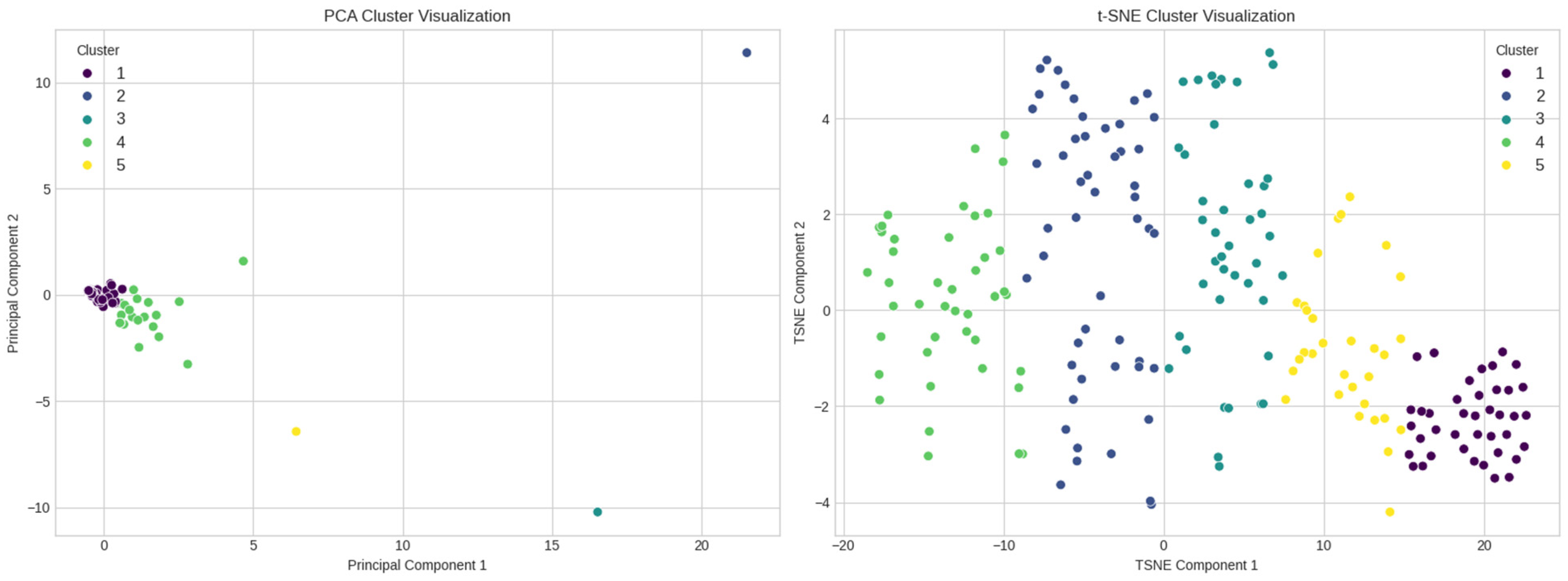
5.1. Clustering for Total CO₂ Emissions

Based on the optimal clusters obtained through K-means, the results for PCA and t-SNE in CO₂ clustering emissions are shown in Figure 7. The PCA visualization represents the data in a new two-dimensional space created by the first two principal components.

The first principal component explains about 69.95% of the total varianceshowing that this single dimension captures over two-thirds of the variability in CO₂ emission data. This suggests a dominant pattern or factor affecting CO₂ emissions across countries, reflecting a combination of related variables like economic development, industrialization level, or energy consumption patterns. The second principal component accounts for around 25.66% of the variance, representing other significant factors influencing emissions, such as differences in energy sources, policy approaches, and geographical factors among countries. These two components explain approximately 95.61% of the total variance, allowing PCA to reduce the multidimensional dataset to just two dimensions while retaining over 95% of the original information. This reduction reveals solid and consistent patterns in global CO₂ emissions, which can be identified and potentially addressed through targeted policies. Therefore, a simple two-dimensional plot can reveal complex global CO₂ emission patterns while capturing most data variability.

In practical terms, this means that the PCA visualization provides a highly informative representation of the original dataset with very little loss of information. It allows us to understand and communicate the complex patterns of global CO₂ emissions using a simple two-dimensional plot, while still capturing the vast majority of the variability in the data.

The data are clustered for PCA as follows: cluster 1 is the most prominent one, and includes a diverse group of countries, ranging from small island nations to developed European countries. The common characteristic is that these countries have relatively low or average emission profiles. This diversity suggests that absolute emission levels are not the only factor in this clustering; emission intensity or per capita emissions might also play a role. See Appendix B for countries that are grouped in CO₂ emissions.

Cluster 2 contains only China, indicating its unique emission profile. This isolation reflects China’s status as the world’s largest CO₂ emitter, with a scale of emissions that sets it apart from other nations. At the same time, cluster 3 contains only the USA, another major emitter with a unique profile. The separation of China and the USA into individual clusters accentuates their enormous and differentiated impact on global emissions.

Cluster 4 includes major economies and significant emitters like India, Japan, Germany, and Brazil. These countries share characteristics of substantial total emissions due to their large economies or populations but with varying emission intensities. Cluster 5 includes only Russia, suggesting its distinct emission profile, possibly due to its large landmass, cold climate, and energy-intensive economy.

For t-SNE, cluster 1 primarily consists of small island nations and microstates. These countries likely have very low total emissions due to small populations and limited industrial activity. Cluster 2 includes a mix of developed and developing nations, many with significant industrial or energy sectors (e.g., Belgium, Kuwait, Norway). This cluster might represent countries with moderate to high emissions but varying efficiency levels.

Cluster 3 comprises many developing countries and some Eastern European nations. These countries share characteristics of growing economies with increasing but still relatively low emissions. However, cluster 4 holds the world’s largest economies and emitters, including China, USA, India, and Russia. This cluster represents countries with high total emissions, though the reasons (population size, industrial base, or energy mix) may vary.

Finally, cluster 5 encloses a diverse group of smaller countries, many of which are developing nations or small island states. This cluster might represent countries with unique emission profiles that do not fit neatly into the other categories, possibly due to specific economic or geographical factors.

In summary, the t-SNE visualization provides a more nuanced clustering, capturing non-linear relationships that the PCA might miss. For example, it groups significant emitters like China and USA (cluster 4), while PCA separates them. This suggests that t-SNE identifies similarities in emission patterns beyond the emissions scale.

The differences between PCA and t-SNE clustering highlight the complexity of global emission patterns. While PCA focuses on the most significant linear relationships, t-SNE captures more subtle, non-linear similarities between countries’ emission profiles. This multifaceted analysis provides a richer understanding of the factors influencing CO₂ emissions across different nations. The results obtained in both techniques are shown in

Table 4. PCA and t-SNE for CO₂ clustering of emissions. Source: Authors’ own elaboration with data from OWD.

Cluster PCA	CO2	Cement	Coal	Flaring	Gas	Oil
1	35.7394	1.6005	10.9583	0.4139	9.5240	13.0532
2	10,173.2746	761.5619	7424.0688	3.9222	469.4575	1353.8085
3	5297.2622	38.2838	1402.0755	61.3207	1507.0304	2260.4330
4	535.0613	18.2968	172.0646	10.0039	123.5781	208.3561
5	1665.7432	22.8961	401.1005	49.4200	795.1316	380.9303
Cluster t-SNE	CO2	cement	coal	flaring	gas	oil
1	0.2682	0.0034	0.0006	0.0000	0.0014	0.2628
2	42.2721	1.5699	8.8626	0.5327	11.4048	19.6092
3	10.6192	0.8461	3.4490	0.0139	0.6759	5.6263
4	749.3502	32.1408	331.0221	8.6567	151.0933	219.8762
5	2.3122	0.0679	0.5565	0.0120	0.0216	1.6541

.

Table 4 divides countries into different clusters based on their emissions. Cluster 1 includes most countries in the world with relatively low emissions in all categories. These countries have a lower carbon footprint, which could indicate smaller economies, less industrialization, or more sustainable energy and environmental policies. Cluster 2 contains only China, which has significantly high emissions in all categories, reflecting China’s status as an industrial superpower with high manufacturing output and energy consumption. Cluster 3 only contains the USA, which has high CO₂, gas, and oil emissions, consistent with the large size of the USA economy, its dependence on oil and gas for energy, and its high-consumption lifestyle. Cluster 4 includes large and diverse economies with significant industrial sectors but stricter emissions policies. Finally, Group 5 only contains Russia, which has moderate levels of emissions in all categories, reflecting its position as a natural resource-rich country with a significant oil and gas export economy.

In contrast, in t-SNE, Cluster 1 includes small island nations and low-population countries with lower industrial capacity, smaller economies, and dependence on energy imports. Their contributions to global emissions are likely minimal, which explains their clustering. Cluster 2 includes a mix of developing and developed countries; several have developing or transition economies and may have evolving environmental and energy policies. This group reflects the complexity of emissions profiles, with some countries having intensive industries and others on the path to energy modernization. Cluster 3 is diverse, including developing countries and some with recent economic advances. Several nations face development challenges that could influence their emission profiles, such as economic growth and sustainable energy strategies. Countries like Costa Rica, known for their environmental policies, suggest a mix of emission strategies within the cluster.

Cluster 4 comprises the world’s largest and most industrialized economies, including many OECD countries and large emitters such as China, the US, and Russia. As mentioned before, these countries have a combination of high industrial capacity, high levels of energy consumption, and varying environmental policies. They contribute significantly to global emissions. Finally, Cluster 5 contains a variety of countries, many of which are developing nations. The presence of countries like Bhutan, which strongly focus on sustainability, suggests that per capita emissions may be low to moderate but with different development contexts and energy policies. The t-SNE analysis provides insights into how countries with similar emission profiles or development contexts cluster in the data space.

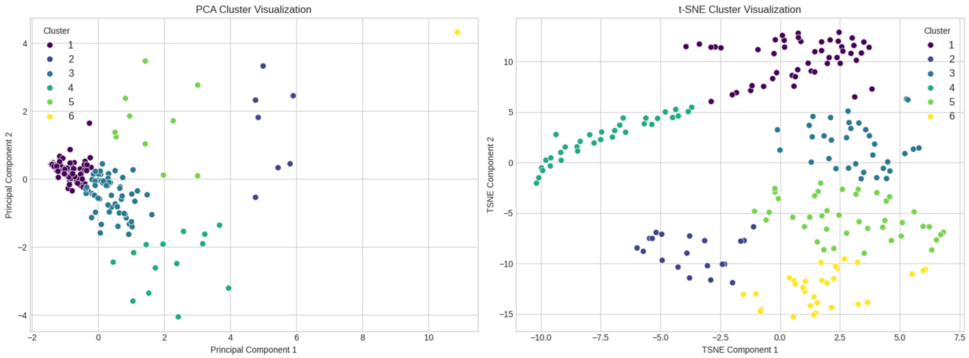
5.2. Clustering for CO₂ per Capita Emissions

The results obtained for per capita emissions are also interesting. In PCA, the first principal component explains 46.22% of the total variability in the data, while the second principal component adds 17.686% to the variance explanation, bringing the total variability captured by both components up to approximately 63.92%. On the other hand, the t-SNE visualization shows a more precise separation and dispersion of the clusters, as can be seen in Figure 8.

Table 5. PCA and t-SNE for CO₂ per capita clustering of emissions. Source: Authors’ own elaboration with data from OWD.

Cluster PCA	CO2	Cement	Coal	Flaring	Gas	Oil
1	1.4088	0.0475	0.1239	0.0158	0.1705	1.0508
2	14.0735	0.2184	5.5503	0.1023	1.4771	6.6421
3	22.5878	0.3836	0.2800	0.4519	14.8261	6.6463
4	39.4083	0.7862	0.0000	0.9169	33.7095	3.9958
5	6.3762	0.1661	1.2870	0.0372	1.0818	3.7599
6	7.4975	0.1525	0.4782	0.6630	3.2760	2.9102
Cluster t-SNE	CO2	cement	coal	flaring	gas	oil
1	0.4751	0.0095	0.0379	0.0129	0.0244	0.3904
2	12.8029	0.1922	0.4815	0.5721	7.9014	3.6309
3	1.3355	0.0873	0.2785	0.0043	0.1556	0.8098
4	6.3349	0.0012	0.0084	0.0000	0.1815	6.1437
5	4.2287	0.2231	0.5766	0.0338	1.1025	2.2598
6	10.4276	0.2389	4.4099	0.0869	2.0267	3.5913

shows the key results for clustering of CO₂ per capita emissions. Six distinct clusters are considered based on their Calinski–Harabasz and Davies–Bouldin scores; see Appendix C for countries that are grouped in CO₂ per capita emissions. Low general emissions characterize cluster 1, consisting of a diverse range of developing and emerging countries from Africa, Asia, and Latin America, such as Nigeria, India, and Brazil. The average CO₂ of this cluster is 1.41, and it uses little cement and coal and has moderate oil and gas emissions. Cluster 2, on the other hand, exhibits high gas and oil emissions, including oil-rich Middle Eastern countries like Saudi Arabia and the United Arab Emirates. This cluster has very high gas (1.48) and oil (6.64) emissions, in addition to significant carbon emissions. This cluster is distinguished for its high dependency on fossil energy resources.

Cluster 3 comprises developed countries and some advanced economies in Europe, Asia, and North America, including Germany, UK, and USA. This cluster includes high gas emissions (14.83) and reliance on natural gas. Cluster 4 has high industrial emissions, including large industrialized and emerging economies such as China, USA, and Australia, with high gas emissions (33.71). This cluster reflects the intensive use of energy resources in heavy industrial sectors. Cluster 5 has diversified moderate CO₂ from cement and gas emissions, and includes diversified economies such as Canada, Russia, and Venezuela. Finally, cluster 6 consists only of Qatar. This cluster highlights significant flaring emissions, a byproduct of the oil industry.

Cluster analysis of the t-SNE results shows that countries can be grouped into six clusters based on their emissions per capita of CO₂ and other gases. Cluster 1 mainly includes developing countries in Africa and Asia, such as Ethiopia, Nigeria and Uganda. These countries have low CO₂ and other gas emissions due to minimal industrialization and energy infrastructure. Cluster 2 includes countries rich in natural resources, some industrialized countries such as Canada and Russia, and Gulf countries like Saudi Arabia. These countries have high carbon consumption per capita and high CO₂ emissions, indicating their high energy demand. Cluster 2 contains developed and emerging economies in Europe and Latin America, such as Spain, Mexico, and Brazil, with moderate CO₂ and various other gas emissions, reflecting a diversity of energy sources.

In contrast, cluster 3 includes developing and emerging countries from multiple regions, such as India, Colombia, and the Philippines, with moderate CO₂ emissions and a low profile in most other gases, indicating a mild dependence on fossil energy. Cluster 4 incorporates low-emitting countries such as tourist paradises and small islands like the Seychelles and Malta, with low per capita and predominant oil consumption, suggesting a dependence on transportation and tourism-related activities. Finally, cluster 5 comprises developed and emerging economies in Europe and Latin America, such as Spain, Mexico, and Brazil, with moderate CO₂ and other gas emissions, reflecting a diversity of energy sources with a significant emphasis on the energy sector. The findings offer considerable knowledge about global emission trends and energy consumption patterns.

The t-SNE visualization shows a more precise separation and dispersion of clusters compared to PCA, capturing non-linear relationships and providing a detailed representation of CO₂ emissions patterns. While PCA efficiently groups the most polluting countries based on linear relationships, t-SNE reveals complex patterns related to population, urbanization, industrial capability, and fossil fuel dependence. This comprehensive analysis, combining K-means clustering with PCA, and t-SNE, highlights significant disparities in CO₂ emissions among countries, both in absolute and per capita terms.

The findings align with the existing literature, confirming China, USA, and Russia as the highest absolute emitters, and Qatar leading in per capita emissions [10,20]. These results highlight the importance of region-specific approaches to emission reduction and emphasize the need for international collaboration and coherent global policies. The understandings gained from this multifaceted analysis are crucial for policymakers in designing targeted climate change mitigation strategies, considering the emission profiles and underlying factors of different countries [9,14].

6. General Discussion

The application of PCA and t-SNE techniques has offered complementary insights. While PCA effectively identified the most significant contributors to global emissions, t-SNE revealed more nuanced relationships among countries, capturing non-linear interactions between factors such as population, urbanization, and industrial capability. These findings emphasize the complexity of the emissions landscape and the need for multifaceted approaches to emission reduction.

The disparities in emissions between developed and developing nations, as well as between urban and rural areas within countries, point to the importance of considering equity and fairness in climate policy. Future international agreements may need to account for these differences, potentially through mechanisms such as differentiated responsibilities or support for low-carbon development in emerging economies.

Finally, the empirical findings emphasize the need for tailored, data-driven approaches to emission reduction. The global nature of climate change requires international cooperation, but the heterogeneity in emission profiles demands nuanced, context-specific strategies. By leveraging advanced analytical techniques such as those employed in this study, policymakers and researchers can develop more effective and equitable approaches to the critical challenge of mitigating global CO₂ emissions.

7. Conclusions

The analysis of CO₂ emissions among 208 countries using K-means clustering combined with PCA and t-SNE visualization has revealed significant patterns and disparities in global carbon emissions. These findings carry important implications for climate change mitigation strategies and international environmental policy. The results obtained indicate that a small number of countries, notably China, USA, and Russia, are responsible for a disproportionate share of global CO₂ emissions. This concentration of emissions suggests that targeted interventions in these nations could yield substantial reductions in global carbon output. However, when emissions are considered on a per capita basis, a different picture emerges. Countries such as Qatar and other Gulf states show the highest emissions per capita, highlighting the role of oil industries and high-consumption lifestyles in driving carbon emissions. The clustering analysis shows that countries can be grouped based on their emission profiles, reflecting similarities in economic structure, energy sources, and development stages. This categorization provides a framework for tailoring emission reduction strategies to specific country groups, potentially increasing the effectiveness of international climate agreements.

Looking ahead, several avenues for future research can be identified. The following are examples: (1) longitudinal studies to analyze how countries’ emission profiles change over time, which could provide insights into the effectiveness of various policy interventions; (2) inclusion of other economic and social factors, such as economic growth, technological adoption, and social indicators, to better understand the drivers behind emission patterns; (3) development of predictive models based on the identified clusters, which could help forecast future emission trends under various policy scenarios; (4) sub-national analysis, applying similar clustering techniques to regions or cities within countries, which could reveal intra-national patterns and identify localized emission reduction strategies; and (5) assessment of policy effectiveness and evaluation of how countries within the same cluster respond to similar policy interventions, which could yield valuable information for climate governance.

References

1. Liu, X.; Zhao, M.; Miao, Q. Global carbon dioxide emissions analysis based on time series visualization. Front. Phys. 2023, 11, 1201983. [Google Scholar] [CrossRef]
2. Kahn, M.E.; Mohaddes, K.; Ng, R.N.; Pesaran, M.H.; Raissi, M.; Yang, J.C. Long-term macroeconomic effects of climate change: A cross-country analysis. Energy Econ. 2021, 104, 105624. [Google Scholar] [CrossRef]
3. Wu, D.; Lin, J.C.; Oda, T.; Kort, E.A. Space-based quantification of per capita CO2 emissions from cities. Environ. Res. Lett. 2020, 15, 035004. [Google Scholar] [CrossRef]
4. Aller, C.; Ductor, L.; Grechyna, D. Robust determinants of CO2 emissions. Energy Econ. 2021, 96, 105154. [Google Scholar] [CrossRef]
5. Ruiz-Alemán, M.E.; Carbajal de Nova, C.; Venegas-Martínez, F. On the nexus between economic growth and environmental degradation in 28 countries classified by income level: A panel data with an error-components model. Int. J. Energy Econ. Policy 2023, 13, 523–536. [Google Scholar] [CrossRef]
6. Valencia-Herrera, H.; Santillán-Salgado, R.J.; Venegas-Martínez, F. On the interaction among economic growth, energy-electricity consumption, CO2 emissions, and urbanization in Latin America. Rev. Mex. Econ. Finanz. 2020, 15, 745–767. [Google Scholar] [CrossRef]
7. Inekwe, J.; Maharaj, E.A.; Bhattacharya, M. Drivers of carbon dioxide emissions: An empirical investigation using hierarchical and non-hierarchical clustering methods. Environ. Ecol. Stat. 2020, 27, 1–40. [Google Scholar] [CrossRef]
8. Salazar-Núñez, H.F.; Venegas-Martínez, F.; Tinoco Zermeño, M.Á. Impact of energy consumption and carbon dioxide emissions on economic growth: Cointegrated panel data in 79 countries grouped by income level. Int. J. Energy Econ. Policy 2020, 10, 218–226. [Google Scholar] [CrossRef]
9. Polat, M.; Kara, K.; Yalcin, G.C. Clustering countries on logistics performance and carbon dioxide (CO2) emission efficiency: An empirical analysis. Bus. Econ. Res. J. 2022, 13, 221–238. [Google Scholar] [CrossRef]
10. Kagawa, S.; Suh, S.; Hubacek, K.; Wiedmann, T.; Nansai, K.; Minx, J. CO2 emission clusters within global supply chain networks: Implications for climate change mitigation. Glob. Environ. Chang. 2015, 35, 486–496. [Google Scholar] [CrossRef]
11. Shah, S.A.; Ye, X.; Wang, B.; Wu, X. Dynamic Linkages among Carbon Emissions, Artificial Intelligence, Economic Policy Uncertainty, and Renewable Energy Consumption: Evidence from East Asia and Pacific Countries. Energies 2024, 17, 4011. [Google Scholar] [CrossRef]
12. Mehboob, M.Y.; Ma, B.; Sadiq, M.; Zhang, Y. Does nuclear energy reduce consumption-based carbon emissions: The role of environmental taxes and trade globalization in highest carbon emitting countries. Nucl. Eng. Technol. 2024, 56, 180–188. [Google Scholar] [CrossRef]
13. Wang, Q.; Yang, R.; Zhang, Y.; Yang, Y.; Hao, A.; Yin, Y.; Li, Y. Inequality of carbon emissions between urban and rural residents in China and emission reduction strategies: Evidence from Shandong Province. Front. Ecol. Evol. 2024, 12, 1256448. [Google Scholar] [CrossRef]
14. Chen, L.; Gozgor, G.; Lau, C.K.M.; Mahalik, M.K.; Rather, K.N.; Soliman, A.M. The impact of geopolitical risk on CO2 emissions inequality: Evidence from 38 developed and developing economies. J. Environ. Manag. 2024, 349, 119345. [Google Scholar] [CrossRef]
15. Huang, L.; Geng, X.; Liu, J. Study on the spatial differences, dynamic evolution and convergence of global carbon dioxide emissions. Sustainability 2023, 15, 5329. [Google Scholar] [CrossRef]
16. Santillán-Salgado, R.J.; Valencia-Herrera, H.; Venegas-Martínez, F. On the relations among CO2 emissions, gross domestic product, energy consumption, electricity use, urbanization, and income inequality for a sample of 134 countries. Int. J. Energy Econ. Policy 2020, 10, 195–207. [Google Scholar] [CrossRef]
17. Caramia, M.; Stecca, G. Unregulated Cap-and-Trade Model for Sustainable Supply Chain Management. Mathematics 2024, 12, 477. [Google Scholar] [CrossRef]
18. Saxena, A.; Zeineldin, R.A.; Mohamed, A.W. Development of grey machine learning models for forecasting of energy consumption, carbon emission and energy generation for the sustainable development of society. Mathematics 2023, 11, 1505. [Google Scholar] [CrossRef]
19. Kenawy, A.M.E.; Al-Awadhi, T.; Abdullah, M.; Jawarneh, R.; Abulibdeh, A. A preliminary assessment of global CO2: Spatial patterns, temporal trends, and policy implications. Glob. Chall. 2023, 7, 2300184. [Google Scholar] [CrossRef] [PubMed]
20. Qi, Y.; Liu, H.; Zhao, J.; Xia, X. Prediction model and demonstration of regional agricultural carbon emissions based on PCA-GS-KNN: A case study of Zhejiang province, China. Environ. Res. Commun. 2023, 5, 051001. [Google Scholar] [CrossRef]
21. Ritchie, H.; Rosado, P.; Roser, M. CO2 and Greenhouse Gas Emissions. Our World in Data. 2023. Available online: https://ourworldindata.org/co2-and-greenhouse-gas-emissions (accessed on 5 June 2023).
22. Laksmana, D.U.; Wikarya, U. The Role of Natural Gas in Indonesia CO2 Mitigation Action: The Environmental Kuznets Curve Framework. Int. J. Adv. Sci. Eng. Inf. Technol. 2020, 10, 274–285. [Google Scholar] [CrossRef]
23. Saidi, K.; Hammami, S. The impact of CO2 emissions and economic growth on energy consumption in 58 countries. Energy Rep. 2015, 1, 62–70. [Google Scholar] [CrossRef]
24. Calinski, T.; Harabasz, J. A Dendrite method for cluster analysis. Commun. Stat. 1974, 3, 1–27. [Google Scholar] [CrossRef]
25. Davies, D.; Bouldin, D. A Cluster Separation Measure. IEEE Trans. Pattern Anal. Mach. Intell. 1979, PAMI-1, 224–227. [Google Scholar] [CrossRef]
Figure 1. CO2 emissions 2010–2022. Source: Authors’ own elaboration with data from OWD.
Mathematics 12 02591 g001
Figure 2. Year-on-year growth rate of CO2 emissions 2010–2022. Source: Authors’ own elaboration with data from OWD.
Mathematics 12 02591 g002
Figure 3. CO2 emissions per capita 2010–2022. Source: Authors’ own elaboration with data from OWD.
Mathematics 12 02591 g003
Figure 4. Annual growth rates of CO2 emissions per capita 2010–2022. Source: Authors’ own elaboration with data from OWD.
Mathematics 12 02591 g004
Figure 5. Correlation heatmap of CO2 emission and CO2 per capita emissions. Source: Authors’ own elaboration with data from OWD.
Mathematics 12 02591 g005
Figure 6. Elbow method for CO2 emission and CO2 per capita emissions. Source: Authors’ own elaboration with data from OWD.
Mathematics 12 02591 g006
Figure 7. Two-dimensional CO2 clustering of emissions. Source: Authors’ own elaboration with data from OWD.
Mathematics 12 02591 g007
Figure 8. Two-dimensional CO2 clustering of per capita emissions. Source: Authors’ own elaboration with data from OWD.
Mathematics 12 02591 g008