Abstract
The growing interest in solar energy stems from its potential to reduce greenhouse gas emissions. Global horizontal irradiance (GHI) is a crucial determinant of the productivity of solar photovoltaic (PV) systems. Consequently, accurate GHI forecasting is essential for efficient planning, integration, and optimization of solar PV energy systems. This study evaluates the performance of six machine learning (ML) regression models—artificial neural network (ANN), decision tree (DT), elastic net (EN), linear regression (LR), Random Forest (RF), and support vector regression (SVR)—in predicting GHI for a site in northern Saudi Arabia known for its high solar energy potential. Using historical data from the NASA POWER database, covering the period from 1984 to 2022, we employed advanced feature selection techniques to enhance the predictive models. The models were evaluated based on metrics such as R-squared (R2), Mean Squared Error (MSE), Root Mean Squared Error (RMSE), Mean Absolute Percentage Error (MAPE), and Mean Absolute Error (MAE). The DT model demonstrated the highest performance, achieving an R2 of 1.0, MSE of 0.0, RMSE of 0.0, MAPE of 0.0%, and MAE of 0.0. Conversely, the EN model showed the lowest performance with an R2 of 0.8396, MSE of 0.4389, RMSE of 0.6549, MAPE of 9.66%, and MAE of 0.5534. While forward, backward, and exhaustive search feature selection methods generally yielded limited performance improvements for most models, the SVR model experienced significant enhancement. These findings offer valuable insights for selecting optimal forecasting strategies for solar energy projects, contributing to the advancement of renewable energy integration and supporting the global transition towards sustainable energy solutions.
Keywords:
solar irradiance forecasting; machine learning predictive models; feature selection algorithms; renewable energy integration MSC:
62J02; 62J05; 62M10
1. Introduction
The accurate forecasting of solar irradiance is an aspect in the efficient planning, integration, and optimization of solar energy systems. Global horizontal irradiance (GHI) is the key parameter that determines the energy output of solar photovoltaic (PV) systems and the viability of solar energy projects [1]. Precise GHI forecasting is essential for a variety of applications, including solar energy generation scheduling, grid integration, and the management of energy storage systems. Inaccurate GHI predictions can lead to suboptimal decision-making, infeasible solar energy projects, and challenges in maintaining grid stability and reliability. As the global demand for renewable energy continues to grow, the need for accurate and reliable solar irradiance forecasting has become increasingly pressing [2].
Traditionally, a variety of statistical and physical models have been employed for GHI forecasting, ranging from simple linear regression to more complex numerical weather prediction (NWP) models. Lopes et al. [2] assessed the global model of the European Centre for Medium-Range Weather Forecasts (ECMWF) integrated forecasting system (IFS) for GHI and DNI forecasts in southern Portugal. They found good agreement between the model predictions and ground-based measurements for GHI, but limitations in capturing cloud and aerosol effects for DNI. Pereira et al. [3] proposed a corrective algorithm to improve the accuracy of ECMWF GHI forecasts using artificial neural networks (ANNs). The ANN-based algorithm, which also included input from a reference clear sky model, was tested against the original ECMWF forecasts and a persistence model, showing that it successfully improved the model predictions.
However, the inherent complexity and variability of solar irradiance, driven by factors such as cloud cover, atmospheric conditions, and geographical location, have posed significant challenges for these conventional forecasting approaches. In recent years, advancements in machine learning (ML) and data-driven modeling techniques have opened new opportunities for enhancing solar irradiance forecasting accuracy. Regression models, in particular, have shown promise in capturing the nonlinear relationships and complex patterns inherent in GHI data, potentially outperforming traditional statistical and physical models. Several studies explore different ML algorithms and their combinations. Huertas-Tato et al. [4] investigated blending multiple models, including satellite data, WRF-Solar, and ML models, demonstrating improved forecasting accuracy compared to individual models. Garniwa et al. [5] proposed a novel method combining the optical flow method and the Long Short-Term Memory (LSTM) model for intra-day GHI forecasting using satellite data. This approach outperforms conventional models, highlighting the potential of deep learning techniques. Gupta et al. [6] presented a less time-consuming ensemble model with multivariate empirical mode decomposition (MEMD) for GHI forecasting, achieving better accuracy than complex deep learning models. Lee et al. [7] compared various ensemble learning models, including Boosted Trees, Bagged Trees, Random Forest, and Generalized Random Forest, for solar irradiance prediction. They demonstrate the superiority of ensemble methods over single learners. Kumari and Toshniwal [8] proposed a Long Short-Term Memory–Convolutional Neural Network (LSTM-CNN)-based hybrid model for GHI forecasting. This model leverages the strengths of both LSTM for temporal features and CNN for spatial features, achieving high accuracy under diverse weather conditions. Michael et al. [9] introduced a novel deep-learning model using stacked bi-directional LSTM (BiLSTM)/LSTM for solar irradiance forecasting. This model achieves high accuracy for both GHI and Plane of Array (POA) irradiance. Chen et al. [10] used information gain factors to select input variables for deep learning models in solar irradiance forecasting, improving the model’s effectiveness. Weyll et al. [11] explored machine learning methods for medium-term GHI forecasting using data from the Global Data Assimilation System (GDAS). Their findings suggest the potential of integrating global-scale data with local measurements for improved forecasting. Lai et al. [12] introduced a deep learning-based hybrid method for GHI forecasting. This method utilizes deep time-series clustering and a Feature Attention Deep Forecasting (FADF) neural network to achieve high forecasting accuracy. Castangia et al. [13] investigated the effectiveness of using exogenous meteorological data for short-term GHI forecasting. They identify the most relevant input variables and demonstrate the benefits of using them in machine learning models. Cannizzaro et al. [14] presented a methodology for GHI forecasting using a combination of Variational Mode Decomposition (VMD), Convolutional Neural Networks (CNN), and ensemble learning techniques. This approach achieved good accuracy for short-term and long-term forecasts. Gupta et al. [15] proposed a MEMD-PCA-GRU model for GHI forecasting, achieving high accuracy across various locations. Ahmed et al. [16] introduced a hybrid approach using weather classification and CatBoost for GHI forecasting. Their results demonstrate the effectiveness of weather classification in improving forecasting accuracy.
The contribution of this work is described below:
First, this study aims to evaluate the performance of six different regression models—artificial neural network (ANN), decision tree (DT), elastic net (EN), linear regression (LR), Random Forest (RF), and support vector regression (SVR)—in forecasting GHI in a site located in Saudi Arabia. The study is motivated by the need to identify the most accurate and reliable regression approach for solar irradiance prediction in this region, which is characterized by a unique climate and high solar energy potential. The selection of these regression models was motivated by their proven effectiveness and widespread application in the field of solar irradiance forecasting. These models have demonstrated the ability to capture the complexity and nonlinearity inherent in solar irradiance data, which makes them suitable for this application. ANN, RF, and SVR have been widely explored in the literature and shown to outperform traditional statistical models. The inclusion of simpler models, e.g., LR and DT, provides a basis for comparison and helps evaluate the trade-off between model complexity and forecasting accuracy. Additionally, the EN model was chosen for its ability to handle multicollinearity in the input features, which is a common challenge in solar irradiance forecasting.
Second, the key novelty of this study lies in the comprehensive comparative analysis of these regression models used for GHI forecasting, which reveals their respective strengths, limitations, and applicability in the context of GHI forecasting.
Third, previous studies have explored ML models for solar irradiance forecasting, but this research uniquely integrates advanced feature selection methods to enhance the predictive performance of these models.
Finally, focusing on a region with distinct climatic characteristics and high solar energy potential, this study not only provides a rigorous comparative analysis of different ML models but also contributes critical insights into the applicability and optimization of these models for regions with similar environmental conditions. Therefore, by identifying the most accurate and reliable regression model for GHI prediction in Saudi Arabia, this research contributes to the development of optimal forecasting strategies for solar energy systems, supporting the country’s renewable energy goals and promoting a sustainable energy future.
The research flow of this study is structured as follows. Section 1 introduces the importance of accurate forecasts for solar energy systems and presents the relevant literature. Section 2 describes the forecast models utilized in the study and details the data collection and processing. Feature selection using the forward selection method is applied to identify the most influential features. The feature selection method is also described in this section. Section 3 presents the results obtained from the analysis and discusses the findings in the context of forecast accuracy and model performance. Finally, Section 4 concludes the study by summarizing the key findings and providing recommendations for future research.
2. Materials and Methods
The investigation performed in this study provides robust ML prediction models for GHI forecasting. The study begins with an initial analysis and data manipulation using features identified from the existing literature as influential predictors of GHI. Thereafter, six different regression models are trained and tested. Each model is trained on historical GHI data and then tested to evaluate its performance in forecasting future GHI values. Advanced feature selection methods are applied to further refine the feature set. Techniques such as forward selection, backward selection, and exhaustive search are utilized to identify the most relevant variables that enhance the models’ predictive power.
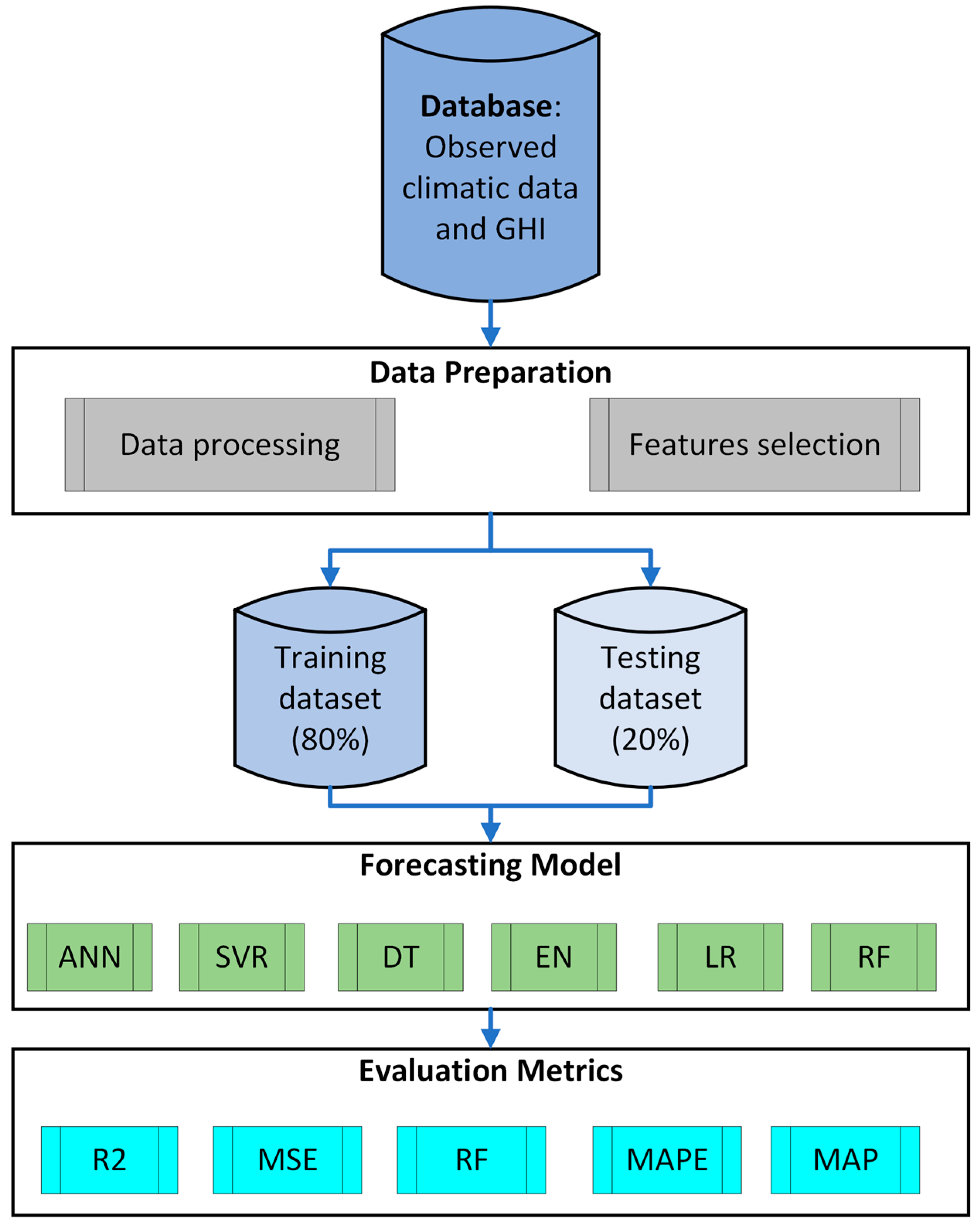
Following the application of feature selection techniques, the models are re-trained and re-tested with the refined feature sets. This step ensures that the models consider the most impactful features for improved accuracy. The evaluation of the predictive accuracy and robustness of each model is measured using metrics such as coefficient of determination or R-squared (R2), Mean Squared Error (MSE), Root Mean Squared Error (RMSE), Mean Absolute Percentage Error (MAPE), and Mean Absolute Error (MAE). This evaluation helps in determining the most effective model for GHI forecasting in the specific climatic conditions of Saudi Arabia. Figure 1 shows the proposed methodology architecture of the research.
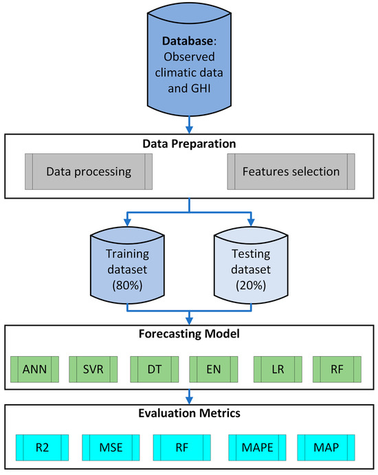
Figure 1.
Schema of the proposed methodology.
2.1. Data Acquisition and Processing
The study focuses on a region in northern Saudi Arabia, specifically at latitude 29.7° and longitude 40°. This site was chosen for its high levels of solar radiation and unique climatic conditions, which make it particularly suitable for solar photovoltaic (PV) systems. Importantly, this area hosts the Sakaka Solar PV Power Plant, Saudi Arabia’s first and largest solar PV project with a capacity of 300 MW [17]. With ongoing efforts to expand solar PV capacity in the region, the location offers a highly relevant and practical context for the study, ensuring that the findings are directly applicable to both current and future solar energy initiatives [17,18].
The meteorology and solar data used in this investigation consist of average monthly measurements spanning the period from 1984 to 2022, retrieved from the NASA POWER website [18]. This comprehensive dataset includes the target variable, GHI, measured in kilowatt-hours per square meter per day (kWh/m2/day). Additionally, it encompasses various features critical to solar irradiance prediction: Direct Normal Irradiance (DNI) in kWh/m2/day, average temperature at 2 m (°C), wind speed at 10 m (m/s), wind speed at 50 m (m/s), relative humidity at 2 m (%), dew point at 2 m (°C), surface pressure (kPa), insolation clearness index, precipitation (mm/day), and surface albedo.
The data preparation and processing were conducted using Python, a powerful programming language well-suited for data analysis and ML. This process involved cleaning the dataset to handle any missing or inconsistent values. Although the dataset in this study has no missing values, it is important to note that there are various techniques to handle missing values if they occur. Examples of such techniques include mean imputation, median imputation, or more advanced methods like k-nearest neighbors (K-NN) imputation, which estimates missing values based on the similarity of neighboring data points.
Data normalization is an essential step to ensure all features are on a comparable scale. We applied the min-max normalization method to scale the data within the range of 0 to 1. The min–max normalization technique was chosen to ensure that all features contribute equally to the model training process, preventing features with larger scales from dominating the learning algorithm. The general mathematical expression for (0, 1) min–max normalization technique is given by Equation (1) [19]:
where x′ is the normalized value, x represents the original value, min(x) is the minimum value of the feature, and max(x) refers to the maximum value of the feature.
Further, the dataset was split into training (80%) and testing (20%) sets to facilitate model evaluation. Various Python libraries, such as Pandas for data manipulation, NumPy for numerical operations, and Scikit-learn for machine learning tasks, were utilized to streamline the data processing workflow. This meticulous preparation ensures that the dataset is ready for accurate and efficient model training and testing, ultimately enhancing the reliability of the GHI forecasting models [20,21].
2.2. Forecasting Models
2.2.1. Artificial Neural Network (ANN)
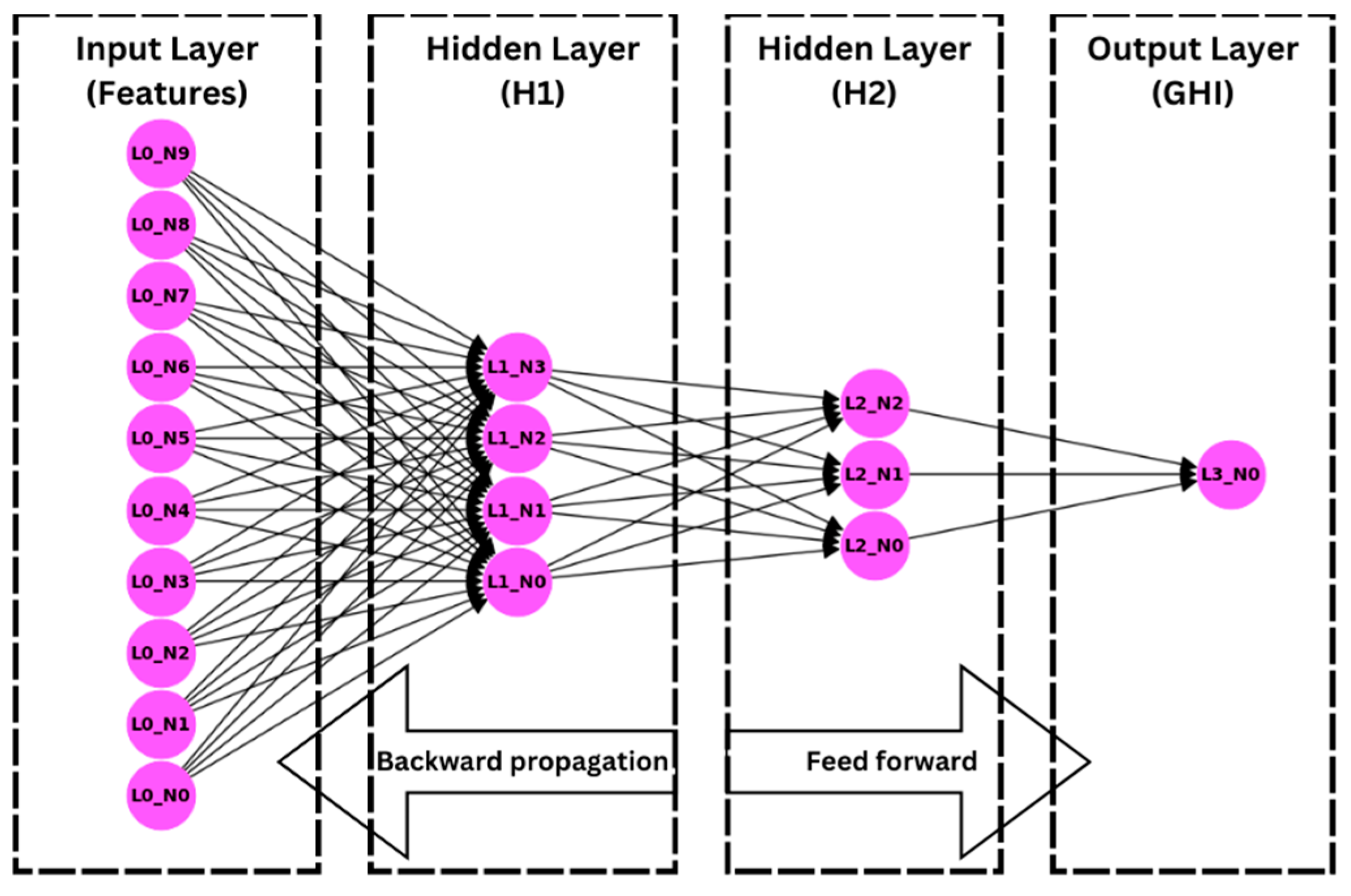
The Artificial Neural Network (ANN) is a computational model inspired by the human brain’s network of neurons. It consists of an input layer, one or more hidden layers, and an output layer. Each layer contains nodes (neurons) connected by weights. The ANN learns to predict outputs from inputs by adjusting these weights through a process called backpropagation [20]. The mathematical expression for a neuron’s output in layer l can be described using Equation (2) [21]:
where is the activation of neuron j in layer l, σ represents the activation function (e.g., sigmoid, ReLU), is the weight between neuron i in layer l − 1 and neuron j in layer l, describes the activation of neuron i in the previous layer, is the bias term for neuron j in layer l.
The network in this study is trained using backpropagation, where the error is computed and propagated backward to update the weights. Figure 2 demonstrates the ANN predictive model architecture that includes an input layer with 10 input features, two hidden layers, and an output layer for the forecasted GHI.
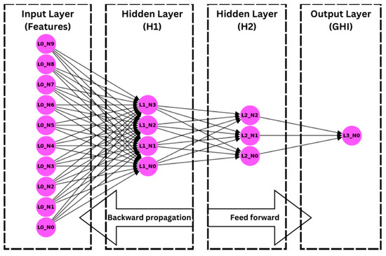
Figure 2.
ANN architecture.
2.2.2. Decision Tree (DT)
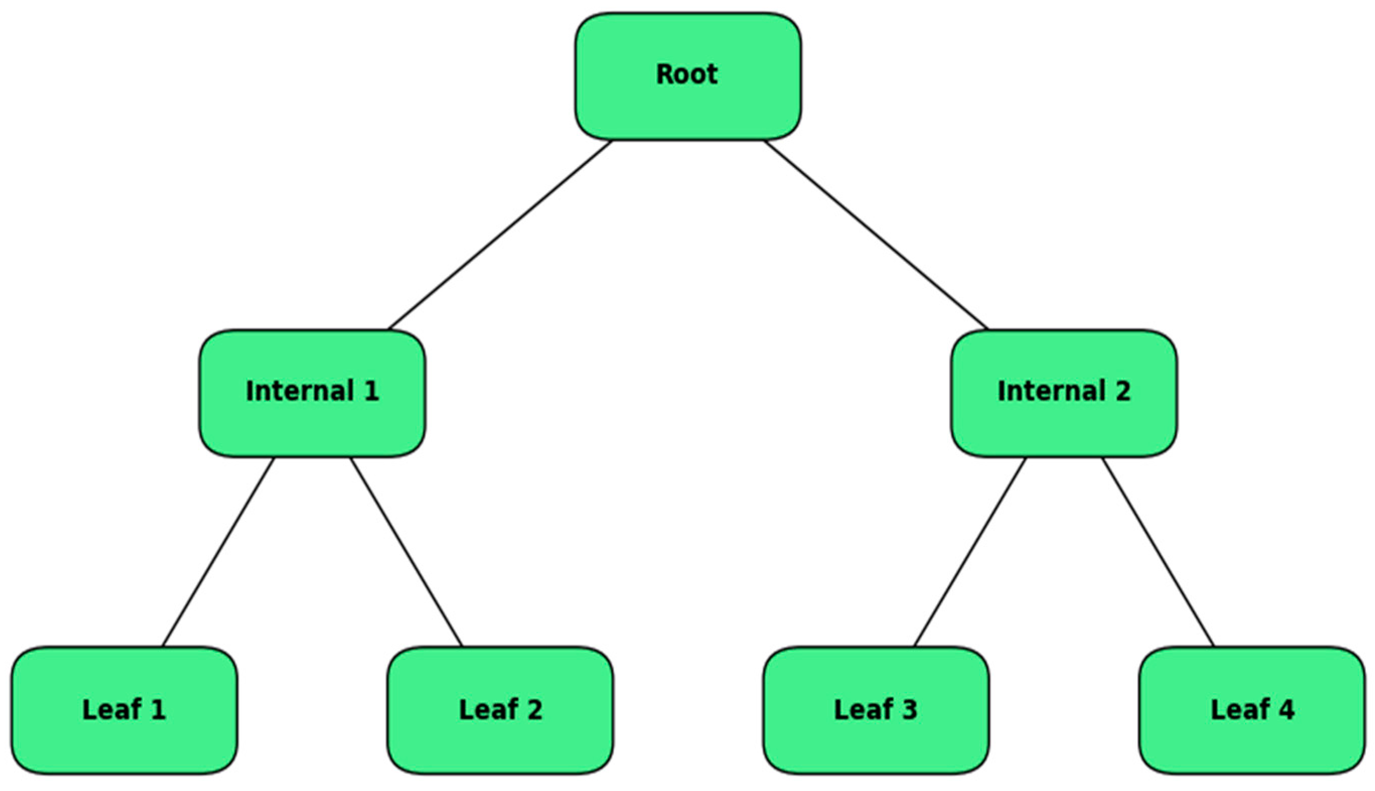
Decision tree Regression is a supervised learning algorithm used to predict continuous values by learning decision rules derived from the data features. The decision tree, as illustrated in Figure 3, is structured as a series of nodes, branches, and leaves, where each internal node represents a decision based on a feature, branches represent the outcomes of those decisions, and leaves represent predicted values [22].
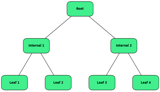
Figure 3.
DT architecture.
The decision tree-building process involves recursively splitting the dataset into subsets to minimize the prediction error by means of variance reduction. This is usually achieved by minimizing the variance of the target variable within each subset. For a given dataset D at a node, the variance of the target variable y is calculated using Equation (3) [23,24,25,26]:
where is the target value of the i-th instance, is the mean of the target values in D, and ∣D∣ is the number of instances in D.
The objective is to find a split that maximizes the reduction in variance. If Dleft and Dright are the subsets resulting from a split, the reduction in variance is measured by Equation (4):
The algorithm selects the split that maximizes ΔVar, thereby reducing the overall prediction error.
Once the tree is constructed, predicting the value for a new instance involves traversing the tree based on the feature values of the instance until reaching a leaf node. The predicted value , as expressed by Equation (5), at a leaf node is typically the mean of the target values of the training instances in that leaf.
where ∣Dleaf∣ is the number of instances in the leaf node and are the target values of those instances.
2.2.3. Elastic Net (EN)
Elastic net (EN) is a regularized regression method that linearly combines the penalties of Lasso (L1) and Ridge (L2) regression. It is particularly useful when dealing with highly correlated predictors. The objective function for the elastic net is expressed by Equation (6) [27]:
where is the vector of coefficients, represents the target value for the i-th data point, is the feature vector for the i-th data point, and are the regularization parameters for L1 and L2 penalties, respectively.
2.2.4. Linear Regression (LR)
Linear regression (LR) is a basic and widely used type of predictive analysis. The objective is to model the relationship between a dependent variable and one or more independent variables by fitting a linear equation to the observed data. The linear regression model is given by Equation (7) [28]:
where y is the dependent variable, X is the matrix of input features, w is the vector of coefficients, and b is the intercept.
2.2.5. Random Forest (LR)
Random Forest (RF) is an ensemble learning method that constructs multiple decision trees during training and outputs the mean prediction (regression) or majority vote (classification) of the individual trees. It reduces overfitting by averaging multiple trees trained on different parts of the data. The prediction for a given input is calculated by Equation (8) [28]:
where represents the number of trees, and is the prediction of the t-th tree.
2.2.6. Support Vector Regression (SVR)
Support vector regression (SVR) is an application of support vector machines (SVM) for regression tasks. SVR attempts to fit a function within a specified margin around the actual observed outputs. The objective is to minimize the coefficients while ensuring the predictions fall within this margin. The optimization problem for SVR can be formulated as in Equation (9) [17]:
where represents the weight vector, b is the bias term, and refer to the slack variables for the i-th data point, the constant C > 0 is the regularization parameter, is the input feature vector.
2.3. Features Selection
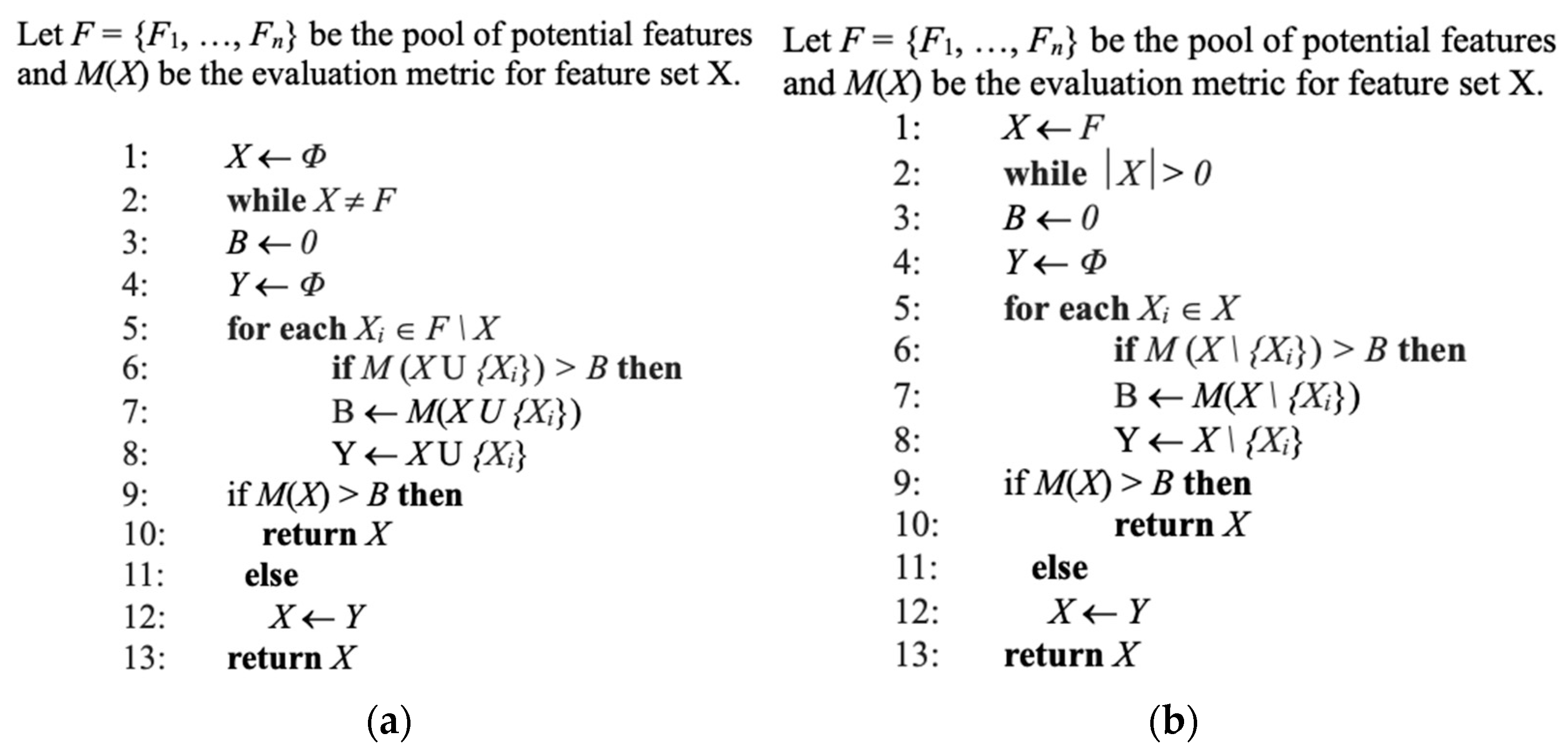
Forward, backward, and exhaustive search feature selection methods are applied to identify the most relevant features that contribute to the predictive performance of the models. Forward feature selection (Figure 4a) is an iterative process that starts with an empty model and adds features one at a time. At each step, the feature that improves the model the most is added. This process continues until no significant improvement is observed [29]. The algorithm can be summarized as follows:
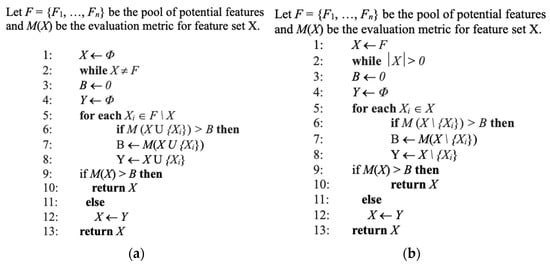
Figure 4.
Forward and backward selection algorithms: (a) forward feature selection algorithm; (b) backward feature selection algorithm. Source: Adapted from Ref. [29].
- Initialize the model with no features;
- For each feature not in the model:
- Temporarily add the feature to the model;
- Evaluate the model using a chosen metric (e.g., cross-validation error).
- Select the feature that most improves the model;
- Repeat steps 2–3 until no significant improvement is achieved or a stopping criterion is met.
Backward feature selection (Figure 4b) starts with all candidates’ features and removes them one at a time. At each step, the feature whose removal least affects the model’s performance is removed [29]. The algorithm can be summarized as follows:
- Initialize the model with all features;
- For each feature in the model:
- Temporarily remove the feature from the model;
- Evaluate the model using a chosen metric (e.g., cross-validation error).
- Select the feature whose removal has the least impact on the model;
- Repeat steps 2–3 until a stopping criterion is met (e.g., a specified number of features remain or no significant improvement is observed).
Exhaustive search evaluates all possible combinations of features to determine the best subset. This method is computationally expensive but guarantees finding the optimal set of features [30]. The algorithm can be described as:
- Generate all possible combinations of features;
- For each combination:
- Train the model using the selected combination of features;
- Evaluate the model using a chosen metric (e.g., cross-validation error).
- Select the combination that yields the best performance.
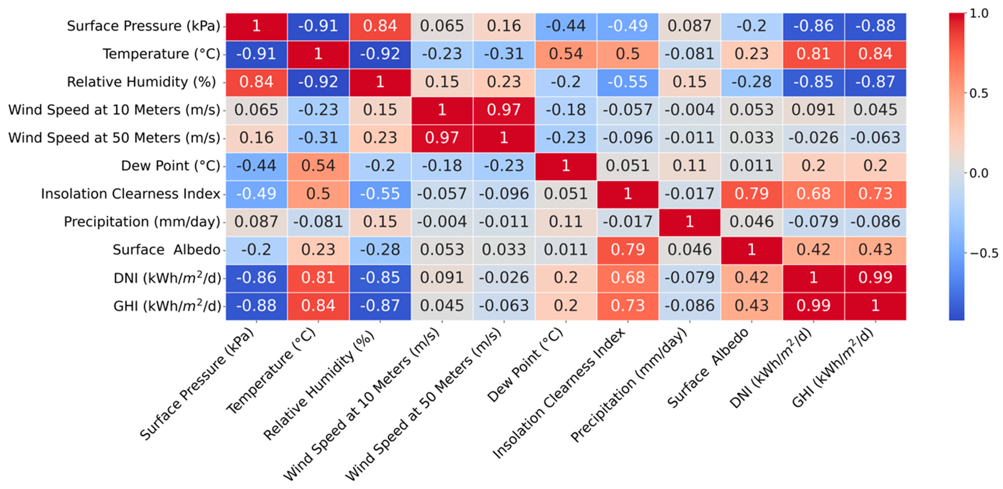
Forward feature selection identified temperature, insolation clearness index, and DNI as the most relevant features. Similarly, both backward feature selection and exhaustive search methods converged on the same set of features: temperature, relative humidity, insolation clearness index, and DNI. Notably, surface pressure, which ranked second in correlation with the target variable (GHI), as shown in Figure 5, was not selected by any of the feature selection methods. Feature selection methods prioritize relevant features and minimize redundancy and noise. This explains the exclusion of surface pressure, despite its high correlation. It suggests that surface pressure’s contribution to GHI prediction might be captured by the chosen features (temperature, relative humidity, insolation clearness index, and DNI). Additionally, feature selection algorithms might have identified multicollinearity between surface pressure and other features, prioritizing a diverse set of features for a more robust model.
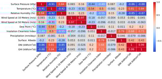
Figure 5.
Features correlation with GHI.
2.4. Evaluation Metrics
Evaluation metrics are fundamental to assessing the performance of machine learning models. The choice of evaluation metric depends on the nature of the problem, such as classification, regression, or clustering. Regression problems, such as the predictive models performed in this study, are typically evaluated using metrics such as MSE, MAE, and R2. Each metric highlights different aspects of model performance; for instance, MSE emphasizes the magnitude of prediction errors. In this study, R2, MSE, RMSE, MAPE, and MAE are calculated to evaluate the accuracy of the predictive models using Equations (10)–(14) [31,32], respectively.
where represents the observed value of GHI, is the predicted value of GHI, and N is the number of observations.
2.5. Cross-Validation
The cross-validation (CV) technique is essential for ensuring that the prediction models perform robustly on unseen datasets. Principally, CV is performed by splitting the data into several groups; one group is used to test the performance of the model, while the other groups are used to train the model. Many iterations are performed to complete the whole process over a specific timeframe, with different groups acting as the test and training datasets [33]. Various techniques are used to validate the accuracy of the model, such as k-fold and shuffle split, which were used in this research.
2.5.1. K-Fold CV Method
In this technique, the data are split into k dataset samples randomly, as illustrated in Figure 6 [34]. One sample out of these k datasets is selected to validate the results, while the remaining k − 1 samples are used as training datasets. The most popular techniques used in the k-fold CV method are 5-fold and 10-fold. The best predicted results for this method are obtained by optimally grouping the testing datasets for validation and training datasets. Additionally, before building the model and selecting samples, it is advised to conduct sanity testing on the dataset to identify missed values and unwanted rows. The quality of the data used for classification is rarely checked in previous research [35]. However, the appropriateness of the data is checked in this work before training the classification model.
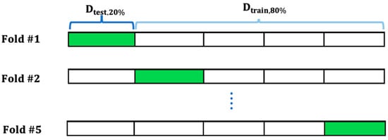
Figure 6.
The ML k-fold CV method in which 20% of the datasets are used for testing, while 80% of the datasets are used for model training.
2.5.2. Shuffle Split CV Method
Shuffle split, also known as the Monte Carlo CV (MCCV) method, is an asymptotically reliable technique in deciding the model number of elements. The over-fitting is eliminated in this method as it does not consider the excessive models with a higher probability of selecting the calibrated model [36]. This method, as in k-fold, splits the data into trained and tested subsamples. Initial splitting of the data into groups is flexible with any percentage; however, at each iteration, the dataset percentages of tested and trained subsamples are to be different. The next phase is to check the accuracy of the model by comparing it with the test dataset. The performance of the model is validated by computing the average test errors for all the iterations as in Equation (15):
where represents the model that is used in the iteration.
3. Results and Discussion
This section discusses the results obtained from forecasting the GHI in Saudi Arabia using six regression models: ANN, DT, EN, LR, RF, and SVR. The performance of these models was evaluated using several accuracy metrics, namely, R2, MSE, RMSE, MAPE, and MAE, as presented in Table 1.

Table 1.
Accuracy evaluation metrics.
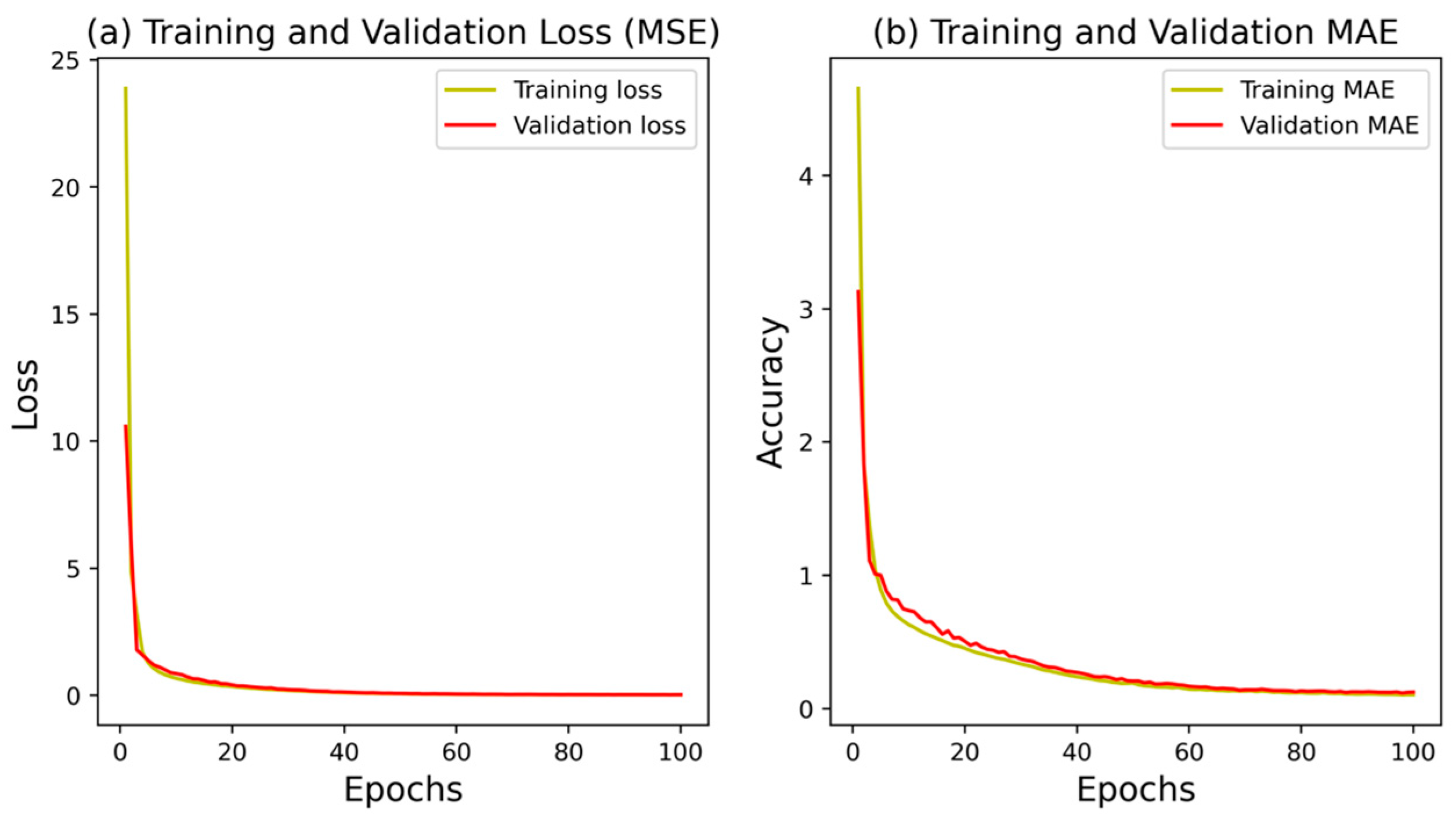
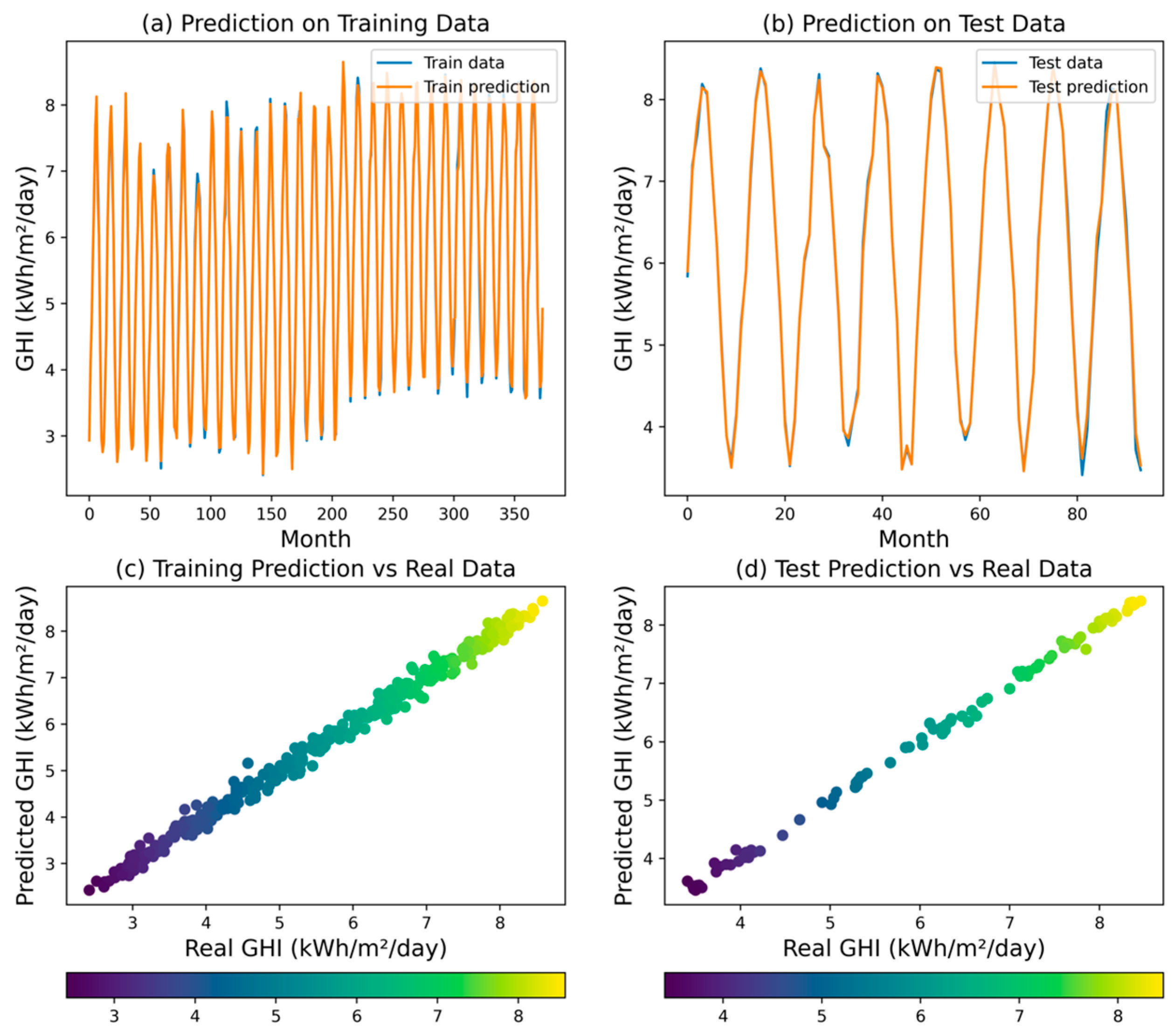
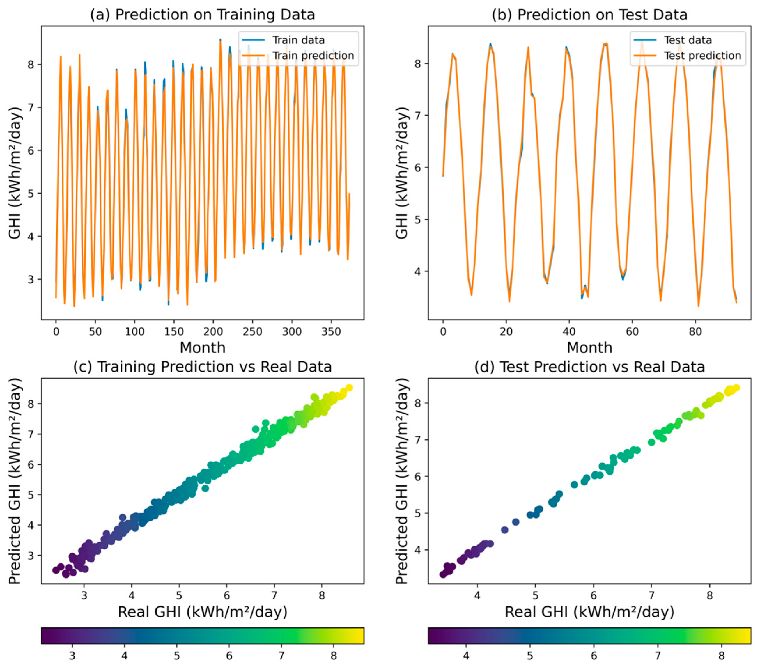
The ANN model achieved an R2 of 0.9976, indicating that 99.76% of the variability in the target variable (GHI) can be explained by the model. The MSE was 0.0065, the RMSE was 0.0803, the MAPE was 0.0102, and the MAE was 0.0567. These results demonstrate that the ANN model was able to provide highly accurate GHI predictions, with low errors across the various metrics. Figure 7 illustrates the training and validation accuracy and loss at each epoch for the ANN model. The convergence of the model indicates that the ANN was effectively and expeditiously trained, achieving a balance between bias and variance. The validation accuracy which follows the training accuracy indicates that the model is not overfitting. This is an important observation as it underscores the robustness of the ANN model in handling the data without becoming too tailored to the training set, which can often lead to poor performance on unseen data. The scatter plot and time series plot of the ANN model’s predictions (Figure 8) further confirm its ability to capture the variations in the GHI values.
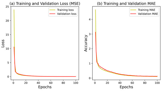
Figure 7.
Training and validation accuracy and loss at each epoch.

Figure 8.
Predicted GHI for ANN model.
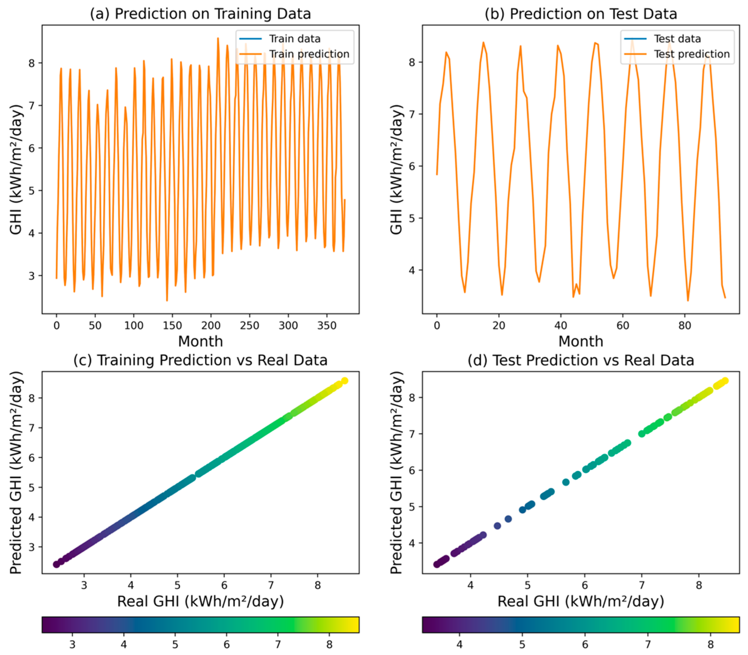
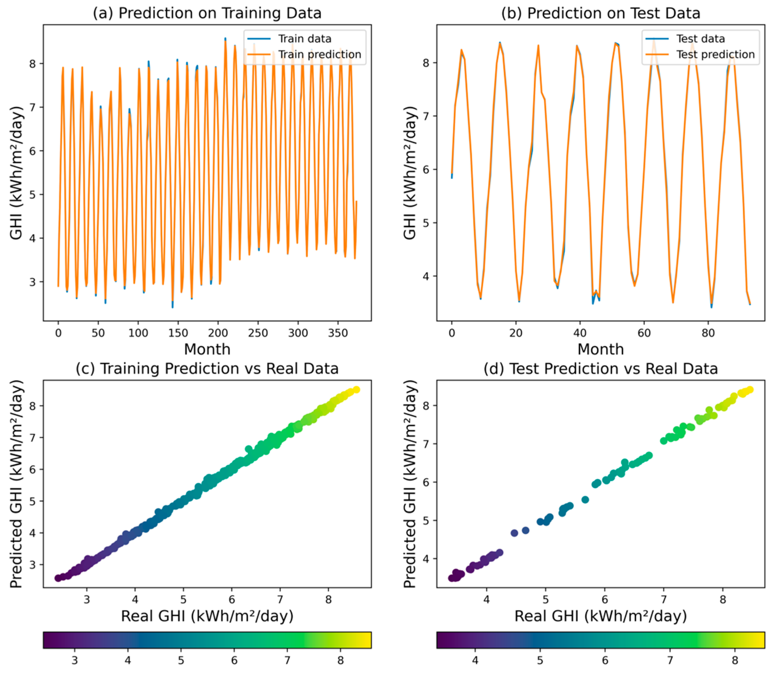
Figure 9 shows that the DT regression model was the most accurate among the models tested. The DT model achieved an R2 value of 1.0, indicating that it was able to perfectly capture the relationship between the input variables and the GHI. The MSE, RMSE, MAPE, and MAE were all 0.0. These performance indicators demonstrate the exceptional predictive performance of the decision tree model, as it was able to fit the training data flawlessly. The high accuracy of the decision tree model can be attributed to its ability to partition the input space into homogeneous regions and assign a constant value (the average GHI) to each region.
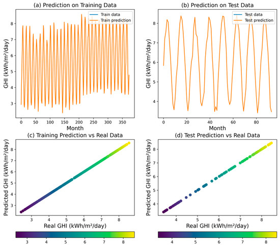
Figure 9.
Predicted GHI for DT model.
The EN regression model exhibited moderate performance in explaining GHI variability, achieving an R2 of 0.8396. While this indicates its ability to capture broad trends, error metrics—MSE (0.4289), RMSE (0.6549), MAPE (0.0966), and MAE (0.5534)—reveal limitations in precisely matching individual data points. Elaborations in Figure 10 corroborate these findings, demonstrating the model’s ability to track the general GHI trajectory but failing to capture finer details. Compared to ANN and DT models, the elastic net appears less adept at precise GHI prediction.
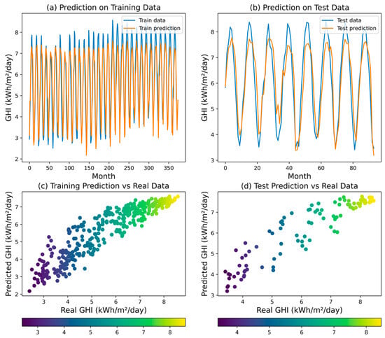
Figure 10.
Predicted GHI for EN model.
The LR model demonstrated strong explanatory power for GHI unpredictability, achieving a high R2 of 0.9986. This translates to capturing over 99.86% of the variance, indicating a good fit for the overall trend. However, examining error metrics reveals limitations in point-to-point prediction accuracy. The MSE of 0.0037, RMSE of 0.0610, MAPE of 0.0086, and MAE of 0.0480 suggest the presence of residual error. Figure 11 perceptibly confirms these observations. Compared to the ANN and DT models, linear regression offers a good balance between interpretability and accuracy, though potentially surpassed by those methods in precise prediction.
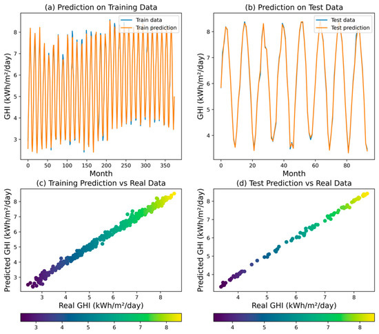
Figure 11.
Predicted GHI for LR model.
The RF regression model demonstrated a remarkable performance reflected by an R2 value of 0.9987, which indicates its ability to explain 99.87% of the variability observed in the GHI. This finding highlights the model’s strong predictive capabilities and its potential for accurately capturing the underlying patterns within the GHI dataset. Assessing the model’s predictive accuracy, MSE was measured at 0.0036, indicating a relatively small average squared difference between the predicted and actual GHI values. The RMSE of the RF model was found to be 0.0599. This metric provides a measure of the typical magnitude of the residuals, further supporting the model’s ability to closely align with the observed GHI values. Moreover, MAPE was calculated at 0.0079, which further substantiates the model’s accuracy by indicating a low average percentage deviation from the observed GHI values.
In addition, MAE was determined to be 0.0438, indicating a small average absolute difference between the predicted and actual GHI values. Figure 12 illustrates the model’s exceptional performance, successfully capturing both the overall trend and finer details of the GHI dataset.

Figure 12.
Predicted GHI for RF model.
The SVR model achieved an R2 of 0.9878, indicating that it was able to explain 98.78% of the variability in the GHI. Examining the error metrics, MSE for the SVR model was calculated at 0.0325. This value suggests a relatively larger average squared difference between the predicted and actual GHI values compared to the ANN, DT, and RF models. Additionally, MAPE was determined to be 0.0238, indicating a moderate average percentage deviation from the observed GHI values. The model’s MAE was measured at 0.1305, signifying a somewhat larger average absolute difference between the predicted and actual GHI values. Figure 13 reveals that the SVR model may not adequately account for the intricacies and subtle fluctuations present in the GHI dataset.
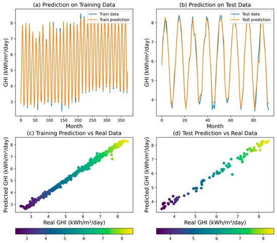
Figure 13.
Predicted GHI for SVR model.
The results of the GHI forecasting analysis using various regression models feature the predictive strength of each approach. The DT model emerged as the top performer with perfect scores across all metrics, indicating its exceptional ability to capture the complex relationship between input variables and GHI. The RF model was closely followed, exhibiting strong predictive power and handling non-linear relationships effectively. The ANN model also showed promising results, demonstrating good accuracy and the ability to learn complex patterns. While the SVR and LR models performed moderately well, the EN model had the least impressive performance. This analysis highlights the importance of model selection and evaluation, as different models have varying strengths and weaknesses depending on the specific problem and data characteristics. The findings suggest that DT and RF are suitable choices for GHI forecasting in Saudi Arabia, offering high accuracy and robustness.
Despite the DT model demonstrating the highest performance in this specific context, it is important to acknowledge that different models may perform variably under different conditions and datasets. The use of multiple models in practice is driven by factors such as robustness, generalizability, and sensitivity to overfitting. For instance, while the DT model may perform exceptionally well in this study, it can be prone to overfitting, particularly with smaller datasets or datasets with high variance. Models such as RF and SVR are often preferred in practice because they tend to be more robust and generalize better across different datasets. Therefore, the inclusion and comparison of various models provide a comprehensive understanding of their strengths and limitations, ensuring that the most suitable model can be selected based on specific project requirements and data characteristics.
3.1. Features Selection Analysis
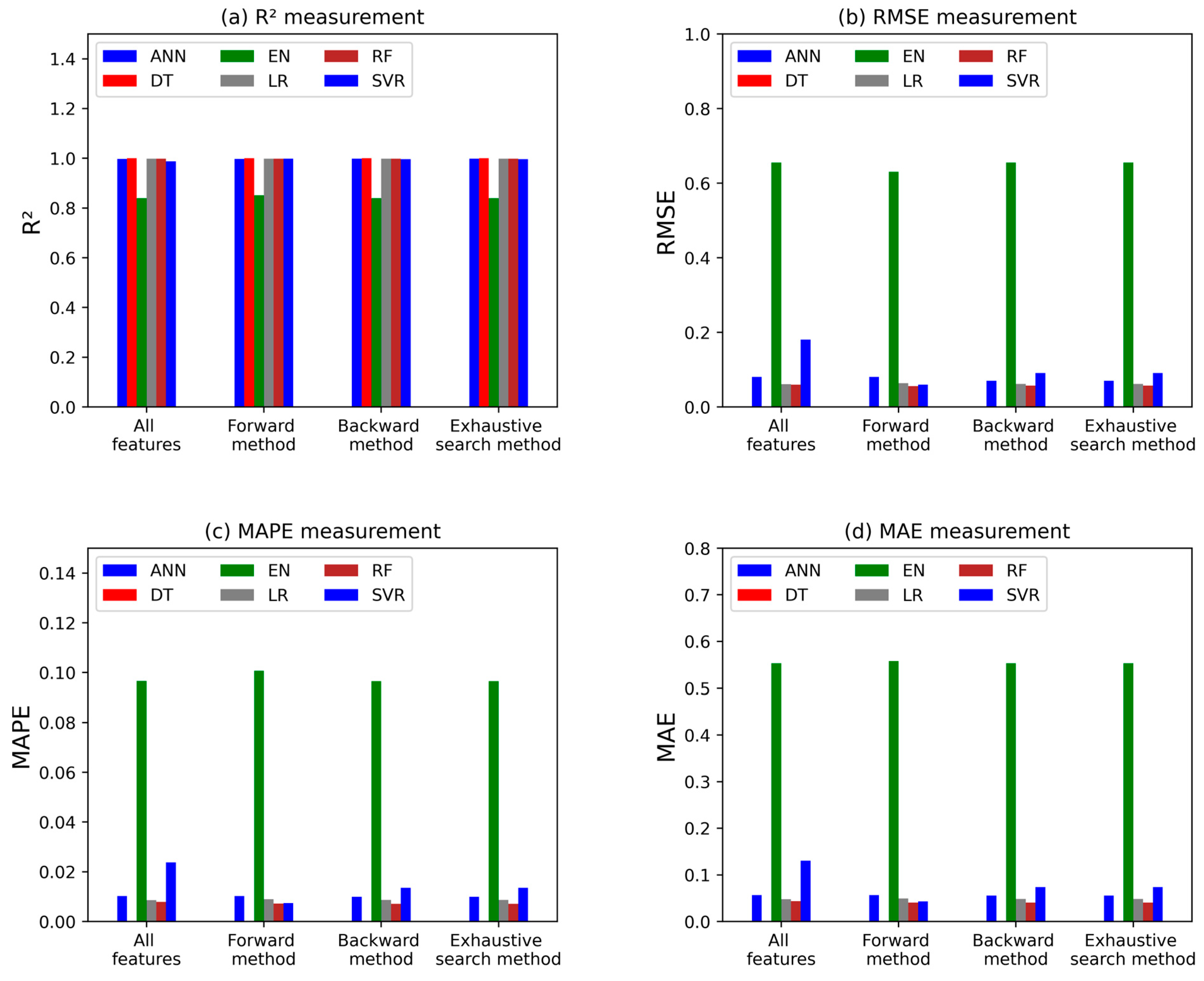
The study also explored the effectiveness of feature selection methods in improving the performance of predictive ML models. While backward selection and exhaustive search yielded the best results for the SVR model, with improvements in R2 and reductions in error metrics, most algorithms showed minimal improvement or no change in performance across all feature selection methods compared to using all features. This suggests that for this particular dataset, feature selection may not be a necessity for all algorithms. Figure 14 and Table 2 compare the different prediction accuracy measures for the forward, backward, and exhaustive feature selection methods with the accuracy of models applying all the features.
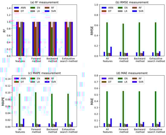
Figure 14.
Accuracy measures of feature selection models.
Table 2.
Accuracy evaluation metrics for the feature selection methods.
3.2. Analysis of K-Fold and Shuffle Splits Cross-Validation
The cross-validation techniques are important to provide a more robust assessment of the models’ performance and to ensure that the results are not biased by the specific train–test split used. Table 3 and Table 4 present the accuracy evaluation metrics for the different machine learning models using k-fold and shuffle split cross-validation, respectively. The results with k-fold split cross-validation, presented in Table 3, provide a more robust assessment of the models’ performance. The DT model maintained its superior performance, with an average R2 of 0.9978, MSE of 0.0055, RMSE of 0.0716, MAPE of 1.09%, and MAE of 0.0589. However, all the models showed a relatively consistent performance, which means that the models were able to generalize better and capture the underlying patterns in the data when k-fold cross-validation was applied.
Table 3.
Accuracy evaluation metrics for k-fold split cross-validation.
Table 4.
Accuracy evaluation metrics for shuffle split cross-validation.
The results of the shuffle split cross-validation, presented in Table 4, provide additional confirmation of the models’ performance and consistency. The overall trends observed in the k-fold split cross-validation are further reinforced, with the DT, ANN, RF, and LR models demonstrating the highest levels of predictive accuracy and robustness. The SVR and EN models, while still exhibiting reasonable predictive capabilities, showed lower average R2 scores compared to the top-performing models. These results suggest that the prediction models are robust and can consistently deliver high-quality predictions, even with different cross-validation approaches. However, the exceptionally consistent performances and accuracy measures of the DT, ANN, RF, and LR models across the different cross-validation methods suggest that these models are well-suited for accurate GHI forecasting in the given context.
Although the results indicate the performance of various machine learning models for forecasting GHI, it is essential to acknowledge the limitations of each model in practical applications.
- Artificial Neural Network: NN: Although the ANN showed promising accuracy, its reliance on a large amount of data for training can be a limitation, especially in regions with sparse historical data. Additionally, ANNs can be prone to overfitting if not carefully regulated, which may affect their generalization to unseen data.
- Decision Trees: DTs are intuitive and easy to interpret; however, they can be sensitive to small variations in the data. This sensitivity may lead to different models with slight data changes, which can hinder their reliability in dynamic climatic conditions.
- Elastic Net: While the EN effectively handles multicollinearity, its performance can be limited by the choice of hyperparameters. Finding the optimal balance between LASSO and Ridge penalties is crucial, and this tuning process can be computationally intensive.
- Linear Regression: LR assumes a linear relationship between predictors and the response variable, which may not capture the complexities of solar irradiance patterns. This simplification can lead to significant errors, particularly in non-linear scenarios.
- Random Forest: RF models, while robust and generally accurate, can suffer from interpretability issues. The ensemble nature of RF makes it difficult to understand the contribution of individual features, which is critical for stakeholders seeking actionable insights.
- Support Vector Regression: SVR is effective in high-dimensional spaces, but its performance can degrade with the presence of noise in the data. Additionally, selecting the appropriate kernel and tuning hyperparameters can be challenging and requires careful validation.
4. Conclusions
The prediction of global horizontal irradiance (GHI) is an important aspect during the development of solar photovoltaic power plants. This study aims to investigate the predictive performance of six machine learning models (ANN, DT, EN, LR, RF, and SVR) in forecasting GHI in the northern part of Saudi Arabia. The meteorology and solar data pertaining to this investigation are the average monthly measurements between 1984 and 2022 and were retrieved from the NASA POWER website. The long-term data span provides a comprehensive and long-term perspective on the meteorological conditions and solar resource characteristics. Average monthly measurements were specifically utilized for the analysis, allowing for a detailed assessment of the variations and trends in meteorological parameters and solar irradiance over the years.
Five evaluation metrics—R2, MSE, RMSE, MAPE, and MAE—were considered to evaluate the prediction accuracy. The results revealed that the DT prediction model outperforms other models across various evaluation measures. The DT model exhibited exceptional performance, achieving an R2 of one and a zero error rate on the employed error evaluation metrics. This remarkable outcome establishes its dominance in terms of accuracy and precision for GHI forecasting. However, ANN, LR, RF, and SVR models also provided reliable predictions with satisfactory overall performance.
The study also investigated the impact of feature selection methods on the performance of the predictive models. Various feature selection techniques, including forward selection, backward selection, and exhaustive search, were employed to identify the most influential features for GHI forecasting. The results indicated that, while backward selection and exhaustive search notably improved the performance of the SVR model, yielding higher R2 values and lower error metrics, the other models showed minimal improvement or no significant change in performance across all feature selection methods. This suggests that for the given dataset, incorporating all features may be more beneficial than applying feature selection for most of the models, except for SVR, where selective feature refinement proved to be advantageous. The major findings of this study can be summarized in the following points:
- DT Model: Achieved perfect accuracy with an R2 value of 1.0 and zero errors across all metrics, highlighting its capability to flawlessly capture the relationship between input variables and GHI;
- ANN, RF, and LR Models: Demonstrated high accuracy with R2 values exceeding 0.99, indicating their strong potential for precise GHI forecasting;
- EN Model: While effective in capturing broad trends, it showed limitations in predicting individual data points accurately, reflected in a lower R2 and higher error metrics compared to other models;
- SVR Model: Performed reasonably well but struggled with capturing finer details and subtle fluctuations, as indicated by a lower R2 value and higher error metrics;
- Feature Selection: Backward selection and exhaustive search improved the SVR model’s performance, but for the majority of the models, using all features was more beneficial, indicating minimal gains from feature selection methods.
These findings underscore the importance of selecting appropriate regression models and feature selection techniques tailored to the specific characteristics of the dataset to achieve high forecasting accuracy in solar irradiance prediction. However, future research could explore the development and testing of hybrid models that combine the strengths of various machine learning algorithms, which could offer new avenues for improving forecast accuracy. Furthermore, expanding the scope of the study to include multiple geographical locations with diverse climatic conditions would help in generalizing the findings and formulating robust forecasting strategies applicable to different solar energy projects globally.
To support the reproducibility of this study, it is worth revealing the specifications of the system used in the analysis. The experiments for this study were conducted using a MacBook Air (M2, 2022) with the following specifications: Apple M2 chip with 8-core CPU and 10-core GPU, 16 GB of unified memory, and 512 GB SSD storage.
Author Contributions
Conceptualization, A.A.I., A.A. and M.M.; methodology, A.A.I.; software, A.A.I.; validation, A.A.I., A.A. and M.M.; formal analysis, A.A.I.; investigation, A.A.I.; resources, A.A.I.; data curation, A.A.I.; writing—original draft preparation, A.A.I.; writing—review and editing, A.A.I., M.M.A.S. and M.M.; visualization, A.A.I., A.A. and M.M.; supervision, A.A. and M.M.; project administration, A.A. and M.M.; funding acquisition, A.A. All authors have read and agreed to the published version of the manuscript.
Funding
This research work was funded by Institutional Fund Projects under grant no. (IFPIP: 1217-135-1443).
Data Availability Statement
The data presented in this study are available in NASA POWER at https://power.larc.nasa.gov/data-access-viewer/, reference number [18]. These data were derived from the following resources available in the public domain: https://power.larc.nasa.gov/data-access-viewer/ (accessed on 3 August 2022).
Acknowledgments
The authors gratefully acknowledge the technical and financial support provided by the Ministry of Education and King Abdulaziz University (KAU), DSR, Jeddah, Saudi Arabia.
Conflicts of Interest
The authors declare no conflicts of interest.
References
- Gao, X.-Y.; Huang, C.-L.; Zhang, Z.-H.; Chen, Q.-X.; Zheng, Y.; Fu, D.-S.; Yuan, Y. Global horizontal irradiance prediction model for multi-site fusion under different aerosol types. Renew. Energy 2024, 227, 120565. [Google Scholar] [CrossRef]
- Lopes, F.M.; Silva, H.G.; Salgado, R.; Cavaco, A.; Canhoto, P.; Collares-Pereira, M. Short-term forecasts of GHI and DNI for solar energy systems operation: Assessment of the ECMWF integrated forecasting system in southern Portugal. Sol. Energy 2018, 170, 14–30. [Google Scholar] [CrossRef]
- Pereira, S.; Canhoto, P.; Salgado, R.; Costa, M.J. Development of an ANN based corrective algorithm of the operational ECMWF global horizontal irradiation forecasts. Sol. Energy 2019, 185, 387–405. [Google Scholar] [CrossRef]
- Huertas-Tato, J.; Aler, R.; Galván, I.M.; Rodríguez-Benítez, F.J.; Arbizu-Barrena, C.; Pozo-Vázquez, D. A short-term solar radiation forecasting system for the Iberian Peninsula. Part 2: Model blending approaches based on machine learning. Sol. Energy 2020, 195, 685–696. [Google Scholar] [CrossRef]
- Garniwa, P.M.P.; Rajagukguk, R.A.; Kamil, R.; Lee, H. Intraday forecast of global horizontal irradiance using optical flow method and long short-term memory model. Sol. Energy 2023, 252, 234–251. [Google Scholar] [CrossRef]
- Gupta, P.; Singh, R. Combining simple and less time complex ML models with multivariate empirical mode decomposition to obtain accurate GHI forecast. Energy 2023, 263, 125844. [Google Scholar] [CrossRef]
- Lee, J.; Wang, W.; Harrou, F.; Sun, Y. Reliable solar irradiance prediction using ensemble learning-based models: A comparative study. Energy Convers. Manag. 2020, 208, 112582. [Google Scholar] [CrossRef]
- Kumari, P.; Toshniwal, D. Long short term memory–convolutional neural network based deep hybrid approach for solar irradiance forecasting. Appl. Energy 2021, 295, 117061. [Google Scholar] [CrossRef]
- Elizabeth Michael, N.; Hasan, S.; Al-Durra, A.; Mishra, M. Short-term solar irradiance forecasting based on a novel Bayesian optimized deep Long Short-Term Memory neural network. Appl. Energy 2022, 324, 119727. [Google Scholar] [CrossRef]
- Chen, Y.; Bai, M.; Zhang, Y.; Liu, J.; Yu, D. Proactively selection of input variables based on information gain factors for deep learning models in short-term solar irradiance forecasting. Energy 2023, 284, 129261. [Google Scholar] [CrossRef]
- Weyll, A.L.C.; Kitagawa, Y.K.L.; Araujo, M.L.S.; da Silva Ramos, D.N.; de Lima, F.J.L.; dos Santos, T.S.; Jacondino, W.D.; Silva, A.R.; Araújo, A.C.; Pereira, L.K.M.; et al. Medium-term forecasting of global horizontal solar radiation in Brazil using machine learning-based methods. Energy 2024, 300, 131549. [Google Scholar] [CrossRef]
- Lai, C.S.; Zhong, C.; Pan, K.; Ng, W.W.Y.; Lai, L.L. A deep learning based hybrid method for hourly solar radiation forecasting. Expert Syst. Appl. 2021, 177, 114941. [Google Scholar] [CrossRef]
- Castangia, M.; Aliberti, A.; Bottaccioli, L.; Macii, E.; Patti, E. A compound of feature selection techniques to improve solar radiation forecasting. Expert Syst. Appl. 2021, 178, 114979. [Google Scholar] [CrossRef]
- Cannizzaro, D.; Aliberti, A.; Bottaccioli, L.; Macii, E.; Acquaviva, A.; Patti, E. Solar radiation forecasting based on convolutional neural network and ensemble learning. Expert Syst. Appl. 2021, 181, 115167. [Google Scholar] [CrossRef]
- Gupta, P.; Singh, R. Combining a deep learning model with multivariate empirical mode decomposition for hourly global horizontal irradiance forecasting. Renew. Energy 2023, 206, 908–927. [Google Scholar] [CrossRef]
- Ahmed, U.; Khan, A.R.; Mahmood, A.; Rafiq, I.; Ghannam, R.; Zoha, A. Short-term global horizontal irradiance forecasting using weather classified categorical boosting. Appl. Soft Comput. 2024, 155, 111441. [Google Scholar] [CrossRef]
- Imam, A.A.; Abusorrah, A.; Marzband, M. Potentials and opportunities of solar PV and wind energy sources in Saudi Arabia: Land suitability, techno-socio-economic feasibility, and future variability. Results Eng. 2024, 21, 101785. [Google Scholar] [CrossRef]
- NASA. NASA Prediction of Worldwide Energy Resources (POWER) Project. Available online: https://power.larc.nasa.gov/data-access-viewer/ (accessed on 3 August 2022).
- Jain, S.; Shukla, S.; Wadhvani, R. Dynamic selection of normalization techniques using data complexity measures. Expert Syst. Appl. 2018, 106, 252–262. [Google Scholar] [CrossRef]
- Lucas, S.; Portillo, E. Methodology based on spiking neural networks for univariate time-series forecasting. Neural Netw. 2024, 173, 106171. [Google Scholar] [CrossRef]
- de Dios Rojas Olvera, J.; Gómez-Vargas, I.; Vázquez, J.A. Observational Cosmology with Artificial Neural Networks. Universe 2022, 8, 120. [Google Scholar] [CrossRef]
- Usman Saeed Khan, M.; Mohammad Saifullah, K.; Hussain, A.; Mohammad Azamathulla, H. Comparative analysis of different rainfall prediction models: A case study of Aligarh City, India. Results Eng. 2024, 22, 102093. [Google Scholar] [CrossRef]
- Pekel, E. Estimation of soil moisture using decision tree regression. Theor. Appl. Climatol. 2020, 139, 1111–1119. [Google Scholar] [CrossRef]
- Thomas, T.; Vijayaraghavan, A.P.; Emmanuel, S. Machine Learning Approaches in Cyber Security Analytics; Springer: Singapore, 2020. [Google Scholar]
- Ye, N. The Handbook of Data Mining Human Factors and Ergonomics; CRC Press: Boca Raton, FL, USA, 2003. [Google Scholar]
- Grąbczewski, K. Meta-Learning in Decision Tree Induction; Springer International Publishing: Cham, Switzerland, 2014; Volume 498. [Google Scholar]
- Nikodinoska, D.; Käso, M.; Müsgens, F. Solar and wind power generation forecasts using elastic net in time-varying forecast combinations. Appl. Energy 2022, 306, 117983. [Google Scholar] [CrossRef]
- Gupta, R.; Yadav, A.K.; Jha, S.K.; Pathak, P.K. Predicting global horizontal irradiance of north central region of India via machine learning regressor algorithms. Eng. Appl. Artif. Intell. 2024, 133, 108426. [Google Scholar] [CrossRef]
- Ballesteros, M.; Nivre, J. MaltOptimizer: Fast and effective parser optimization. Nat. Lang. Eng. 2016, 22, 187–213. [Google Scholar] [CrossRef]
- Alway, A.; Zamri, N.E.; Mansor, M.A.; Kasihmuddin, M.S.M.; Jamaludin, S.Z.M.; Marsani, M.F. A novel Hybrid Exhaustive Search and data preparation technique with multi-objective Discrete Hopfield Neural Network. Decis. Anal. J. 2023, 9, 100354. [Google Scholar] [CrossRef]
- Al-Dahidi, S.; Hammad, B.; Alrbai, M.; Al-Abed, M. A novel dynamic/adaptive K-nearest neighbor model for the prediction of solar photovoltaic systems’ performance. Results Eng. 2024, 22, 102141. [Google Scholar] [CrossRef]
- Al-Ali, E.M.; Hajji, Y.; Said, Y.; Hleili, M.; Alanzi, A.M.; Laatar, A.H.; Atri, M. Solar Energy Production Forecasting Based on a Hybrid CNN-LSTM-Transformer Model. Mathematics 2023, 11, 676. [Google Scholar] [CrossRef]
- Pachouly, J.; Ahirrao, S.; Kotecha, K.; Selvachandran, G.; Abraham, A. A systematic literature review on software defect prediction using artificial intelligence: Datasets, Data Validation Methods, Approaches, and Tools. Eng. Appl. Artif. Intell. 2022, 111, 104773. [Google Scholar] [CrossRef]
- Berrar, D. Cross-Validation. In Encyclopedia of Bioinformatics and Computational Biology; Elsevier: Amsterdam, The Netherlands, 2019; pp. 542–545. [Google Scholar]
- Abrasaldo, P.M.B.; Zarrouk, S.J.; Kempa-Liehr, A.W. A systematic review of data analytics applications in above-ground geothermal energy operations. Renew. Sustain. Energy Rev. 2024, 189, 113998. [Google Scholar] [CrossRef]
- Xu, Q.-S.; Liang, Y.-Z. Monte Carlo cross validation. Chemom. Intell. Lab. Syst. 2001, 56, 1–11. [Google Scholar] [CrossRef]


Disclaimer/Publisher’s Note: The statements, opinions and data contained in all publications are solely those of the individual author(s) and contributor(s) and not of MDPI and/or the editor(s). MDPI and/or the editor(s) disclaim responsibility for any injury to people or property resulting from any ideas, methods, instructions or products referred to in the content. |
© 2024 by the authors. Licensee MDPI, Basel, Switzerland. This article is an open access article distributed under the terms and conditions of the Creative Commons Attribution (CC BY) license (https://creativecommons.org/licenses/by/4.0/).