Abstract
In this article, we propose a new path-conservative discontinuous Galerkin (DG) method to solve non-conservative hyperbolic partial differential equations (PDEs). In particular, the method here applies the one-stage ADER (Arbitrary DERivatives in space and time) approach to fulfill the temporal discretization. In addition, this method uses the differential transformation (DT) procedure rather than the traditional Cauchy–Kowalewski (CK) procedure to achieve the local temporal evolution. Compared with the classical ADER methods, the current method is free of solving generalized Riemann problems at inter-cells. In comparison with the Runge–Kutta DG (RKDG) methods, the proposed method needs less computer storage, thanks to the absence of intermediate stages. In brief, this current method is one-step, one-stage, and fully-discrete. Moreover, this method can easily obtain arbitrary high-order accuracy both in space and in time. Numerical results for one- and two-dimensional shallow water equations (SWEs) show that the method enjoys high-order accuracy and keeps good resolution for discontinuous solutions.
MSC:
65M06; 65N06
1. Introduction
Many fluid problems from the fields of physics and engineering can be described as the conservation laws
in the light of the first principles. Here, denotes the vector of conservative variables, and stands for the tensor of physical flux with and being the physical fluxes in the x- and y-directions, respectively. So far, we can deeply understand most physical movements in nature using the conservation principles. However, in the modeling of compressible multi-phase flow/multi-media flow from aerodynamics, astrophysics, aerospace, petroleum industry, etc., the non-conservative product term (i.e., spatial derivative of unknown solution) appears, thanks to the complex interaction between different phases (media). Therefore, the relevant mathematical model cannot be expressed in the conservative form. Nevertheless, the above fluid problems can be characterized by the quasi-linear non-conservative hyperbolic systems as follows:
with being the system matrix. The block-matrix syntax is used here to give a compact notation of the matrices and . We will provide detailed introductions to and in Section 4.2 for the two-dimensional SWEs. Herein, this system (2) is assumed to be hyperbolic, namely and have m real eigenvalues and a full set of m linearly independent eigenvectors, respectively. In particular, the system (2) will reduce to the hyperbolic systems of conservation laws (1), provided that and are Jacobian matrices of and . This observation implies that the system (2) is suitable to express both conservation laws and non-conservative systems at the same time.
However, the major issue of the system (2) consists in the deficiency of the classical definition of the weak solution in the case of discontinuities. It was not until the appearance of the theory of Dal Maso, Le Floch, and Murat (DLM theory) [1] that this major problem made great progress. The DLM theory gives a definition of the weak solutions to the system (2) by introducing a path to connect two states and in phase space. Subsequently, in view of the DLM theory [1], Castro et al. [2] and Pares [3] developed the path-conservative methods according to the non-conservative hyperbolic systems (2). Actually, the path-conservative methods [2,3] can also be known as the extension of the weak formulation of Roe’s method by Toumi [4].
Later, following the original achievements [1,2], many researchers have made many attempts on the path-conservative methods. Representative research mainly include ADER schemes [5,6], FORCE schemes [7], HLLC Riemann solver methods [8], Osher Riemann solver methods [9], central schemes [10], central-upwind schemes [11,12], the ADER-DG method [13], and so on. For the latest progress and a brief historical review, we refer to [14,15].
The key purpose of this research is to propose a new path-conservative DG method for non-conservative hyperbolic systems (2). The resulting method uses the one-stage ADER approach to realize a high-order temporal discretization, and is called the path-conservative ADER-DG method accordingly. The fundamental idea is to employ the DT procedure [16,17,18] instead of the CK procedure to express the spatiotemporal expansion coefficients of the solution through the low order spatial expansion coefficients. In addition, the DT procedure can enable us to realize local temporal evolution along with arbitrary high-order accuracy. As far as we are concerned, this will be the first attempt at applying the DG method along with the DT procedure for the non-conservative system. Then, we extend the proposal to deal with the SWEs in a non-conservative form. Specifically, Li et al. [13] proposed an ADER-DG method for the SWEs in the form of hyperbolic balance laws. Moreover, Li et al. [19] extended the ADER-DG method to solve the Euler equations in gas dynamics. Herein, the success of the ADER-DG method for the SWEs in a non-conservative form will illustrate the universality of the ADER-DG method.
The structure of this article is as follows: Section 2 illustrates the general framework of the path-conservative ADER-DG method and then applies the resulting method to the 1D SWEs in a non-conservative form. Section 3 deals with the two-dimensional (2D) SWEs using the proposed method. Section 4 implements canonical examples to validate the performance of the proposed method. Finally, Section 5 gives some conclusions.
2. General Formulation of Path-Conservative ADER-DG Method
Herein, we give a general framework for the ADER-DG methods according to the non-conservative system (2). Actually, we first multiply the system (2) by a test function from a given approximation space, then integrate on a space-time cell , and obtain
with as the spatial cell. Afterward, we approximate with as a spatiotemporal polynomial. Since usually shows jumps at inter-cells, we present a path-conservative method to deal with the jumps. In the following, we obtain the DG method for PDE (2): for any test function , the numerical solution satisfies the following equality:
with being the unit outward normal vector at the boundary of the cell .
The DG method (3) uses the ADER approach to realize the temporal discretization. Hence, the DG method (3) is one-step, one-stage, and fully-discrete, accordingly. Therefore, we call the proposed method (3) the ADER-DG method. In addition, to achieve the time integration, we need to realize the local time evolution in the space-time cell from using the DT procedure. The DT procedure will be described at length in Section 2.1.3. Here, is obtained from inside the cell , and is obtained from the outside the cell , respectively. Moreover, the notation stands for the jump terms at inter-cells and satisfies the below requirements [2,3,5]:
- For every and ,
- For every , , and ,
In addition, denotes a sufficiently smooth path connecting the states and . A method satisfying the above conditions is called the path-conservative method.
Moreover, according to [13,19], the conservative equivalent of the proposed ADER-DG method (3) to solve the hyperbolic system of conservation laws (1) is as follows:
with as the numerical flux to approximate the physical flux at inter-cells. For example, people often apply the following simple and efficient Lax–Friedrichs numerical flux , where is an estimate of the maximum wave propagation speed. Actually, the above path-conservative ADER-DG method (3) in the non-conservative form reduces to the conservative ADER-DG method (4) in this situation where the non-conservative system (2) is a conservation law (1), i.e., and are the Jacobian matrices of and , respectively. For this equivalence, Dumbser et al. present a detailed proof under the framework of finite volume schemes [5].
2.1. Applications to 1D SWEs
Based on the general framework of the path-conservative ADER-DG method, we then take 1D SWEs
as an example to illustrate the concrete construction steps of the method (3). Herein, , denote the water depth and the fluid velocity, respectively. The notation represents the bottom topography, and the letter “g” stands for the gravitational acceleration.
Following the strategy in [2], we incorporated the geometrical source term in (5) into the term and obtain the following non-conservative form
where
with being the sound velocity. This kind of operation makes it easy to achieve a well-balanced (WB) method for the system (6).
From a mathematical point of view, the non-conservative system (6) preserves the steady state solutions, which meet
In particular, the lake at rest steady state solutions enjoy the below forms
The traditional methods fail to preserve this steady state exactly and result in non-physical oscillations. Well-balanced (WB) methods [20,21] can preserve the steady state up to the machine accuracy at the discrete level and resolve small perturbations of the steady state even on a relatively coarse mesh [22], then increase the computational efficiency correspondingly.
2.1.1. Notations and Solution Space
Firstly, the spatial domain is discreted into N spatial cells with for . Herein, we take and as the mesh center and size of the cell . Moreover, the maximal mesh size is defined as . Here, we apply as the space-time cell and set
as the approximation space, where denotes a set of space-time polynomials on the space-time cell with a degree up to k.
2.1.2. Construction of 1D Path-Conservative ADER-DG Method
For the 1D system (6), the ADER-DG method (3) is as follows: for , the solution meets the below equality:
Further, Equation (8) also enjoys the below equivalent form
With regard to the jump term at inter-cells, there are different choices, such as
- The Osher jump term:
- The Roe jump term:where denotes the Roe linearization matrix of in some sense defined from [4] by Toumi, i.e., a function meets the below properties:
- -
- For each , the matrix owns m different real eigenvalues
- -
- The compatibility property
- -
- For arbitrary , , the matrix satisfies the below requirementin the light of the generalized Roe property.
In addition, with respect to the absolute value operator of the matrix in (10) and (11), we usually use the following notations:
where is the matrix of right eigenvectors of the matrix , and stands for its inverse.
Up to now, the current method (9) can be considered as the function of a given path in the below form:
Moreover, the function is Lipschitz continuous and meets certain regularity as well as the compatibility condition
In this article, we apply the simple segment path
as in [2,3,5].
2.1.3. The DT Procedure
To build the method (9), we need to realize the local temporal evolution in the space-time cell starting from in advance. The reason for this operation is that we need to obtain the numerical solution in the form of spatiotemporal polynomials in each space-time cell. Then, we can calculate the time integration as well as the space-time integration with high-order accuracy in (9). Actually, to realize this goal, the ADER methods [23,24,25,26,27,28,29] use the CK procedure to repeatedly differentiate the governing PDE and to obtain the temporal derivatives using the spatial ones. To obtain high-order time accuracy, we need high-order temporal derivatives. At this time, the CK procedure will become very cumbersome due to the usage of the chain rules. Dumbser and Munz [29] proposed an efficient algorithm on account of the Leibnize rule. More recently, Dumbser et al. [5,6] and Tang et al. [30] apply the local DG predictor approach [31] to take the place of the CK procedure. More recently, Li et al. developed an ADER-DG method for SWEs using the DT procedure [13].
In this study, we apply the DT procedure rather than the CK procedure. In fact, the DT procedure was originally developed with regard to the nonlinear initial value problems [32,33]. Afterward, Ayaz generalized the DT procedure to the 2D cases [16] as well as the system cases [17]. Kurnaza et al. [18] implemented the generalization to more general n-dimensional cases. In addition, Norman and Finkel [34] applied this procedure to build multi-moment finite volume schemes for the 1D SWEs.
In the following, we give a specific definition of the DT procedure as in [16,17,18]. Assume that a function in the cell at is known, the DT is defined as follows:
Here, denotes the transformed function according to the original function . Actually, represents the expansion coefficients with respect to in a form of truncated Taylor series. Table 1 shows some transformed functions used here.

Table 1.
Transformed functions of some functions.
Then, we specifically illustrate the implementation steps of the DT procedure. Initially, we obtain
using the projection to approximate , as well as in cell .
Subsequently, we exert the DT procedure on both ends of (5) and obtain the following recurrence formulae:
Herein, we use the following auxiliary variables:
Afterward, putting , and into (16), we can recursively acquire
which result in
with in each space-time cell . In addition, we present the detailed algorithm of the DT procedure in Algorithm A1 for a better understanding of this procedure.
Remark 1.
In a word, the key function of the DT procedure is to supply a high-order temporal evolution locally for every space-time cell according to the existing solution .
Remark 2.
The CK procedure directly uses the symbolic expansions of the governing PDE and, at a cost, requires the recomputation of many terms. So, the CK procedure leads to exponential growth according to the complexity. Nevertheless, the DT procedure is relatively simple, along with a predictable complexity.
Remark 3.
In practice, there is no need to apply the DT procedure according to the bottom topography b, because the bottom b only depends on the spatial variable x.
2.1.4. The Slope Limiter
Generally, a slope limiter is indispensable for discontinuous problems. Herein, we use the total variation bounded (TVB) limiter [35,36,37] to control nonphysical oscillations. In fact, we only implement the TVB limiter steps in terms of the numerical solutions excluding the bottom topography , which is independent of the time t. Specifically, we need to identify “troubled cells” (i.e., cells involving discontinuities) on the basis of cell averages , and inter-cell values from at .
For illustrative purposes, we first give some notations
Then, we obtain the below updated values
using the TVB limiter [37] for the variables in (17). Here, is a minmod function with
with . The cell will be identified as a troubled cell provided that
Subsequently, the limited inter-cell values are defined with
Finally, a polynomial is determined in the light of the limited inter-cell values (18) along with the cell averages.
2.1.5. Implementation Details of 1D Path-Conservative ADER-DG Method
For the 1D system (6) and inside one time interval , the specific procedures of the proposed method are as follows:
3. Extension to 2D System
This section generalizes the path-conservative ADER-DG method to handle the below 2D SWEs
with v being the fluid velocity in the y-direction. In addition, the system (19) can be expressed as the non-conservative form
with
Similarly to the form (2), Equation (20) enjoys the below compact form
with .
Herein, the Osher jump term is
The Roe-type jump term reads as follows:
Then, we show the specific implementation steps of the DT procedure for the 2D cases. Initially, we have
to approximate , , , and in each space-time cell .
Suppose that the 2D numerical solutions at are known as follows:
Then, as in the 1D case, the DT idea is again used to build the space-time polynomials in every cell and attain the local temporal evolution accordingly.
Actually, we apply the DT procedure on both ends of (19) and obtain the following recurrence formulae
with
as auxiliary variables.
4. Numerical Results
Herein, we confirm the proposed method using several canonical examples. We use the space-time polynomial of degree up to two (i.e., ) in the approximation space in all calculations. We take the Courant–Friedrichs–Levy (CFL) number as to ensure the numerical stability. In addition, we set the gravitational constant . To save space, we only present the numerical results using the method with Roe-type jump terms because the Roe-type method maintains the WB property.
4.1. 1D System
4.1.1. WB Property Test
Firstly, we apply an example to numerically confirm the WB property as in [38]. The initial conditions are
Specifically, we handle two different bottoms:
The first bottom is smooth and the second is discontinuous.
Table 2 and Table 3 present the errors at according to the two different bottom topographies. We can clearly observe that the , , and errors are all at the level of round-off errors for different precisions, verifying the WB property accordingly even for different bottoms. From the numerical perspective, we verify that the current method can maintain the WB property.
Table 2.
Errors according to the example over the first bottom.
Table 3.
Errors according to the example over the second bottom.
4.1.2. Accuracy Test
Next, we use an example from [38] to confirm the accuracy. The initial data read as
over the bottom .
Table 4 shows the errors and the orders at with different mesh resolutions. From Table 4, we can clearly observe that the third-order convergence is achieved for the current method.
Table 4.
Errors and orders for h and .
4.1.3. Perturbations of a Steady State Water Flow
We apply an example from [39] to test the proposed method for the capability to catch small perturbations. The initial data are
with as a parameter over a bump
With time evolution, the initial perturbation breaks down into two pulses, which move in two different directions, as shown in Figure 1. A good agreement is achieved as in [38,39,40]. Obviously, the two types of pulses are all well resolved. In addition, the downstream-traveling water pulse has already passed the bump. In the figures, we can clearly see that there are no spurious numerical oscillations, verifying the essentially non-oscillatory property of the resulting method.
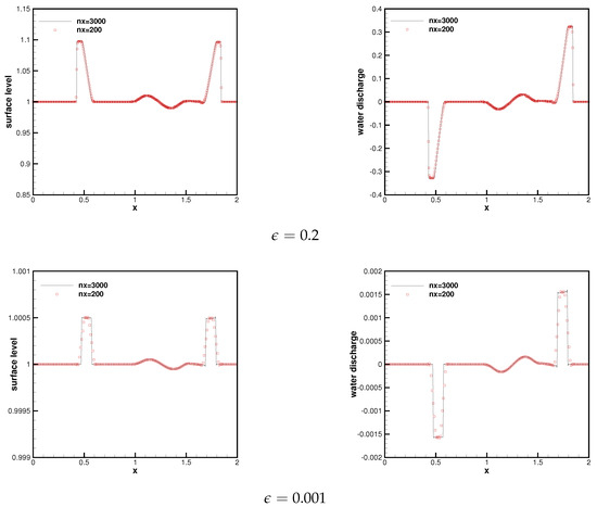
Figure 1.
Surface level (left) and water discharge (right) at .
4.1.4. The Dam Break Problem over a Rectangular Bottom
Next, we handle a dam break problem [40,41,42] and use the below initial data
over a rectangular-like bottom
Figure 2 presents the surface level at as well as . Our method works well for this example, producing well-resolved, non-oscillatory solutions using 500 cells which agree with the converged results using 5000 cells. In addition, the numerical results here can be compared with those from [40,41,42].
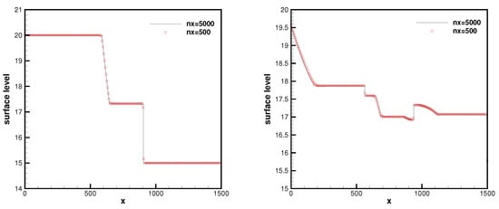
Figure 2.
Surface level at (left) and (right).
4.1.5. Steady Flow over a Hump
Further, we validate this method using a widely-used example [43]. Actually, this example models transcritical and subcritical flows based on the initial conditions
over a hump
Subsequently, we exert different boundary conditions at the ends of the spatial interval.
- Case A: the transcritical flow without a shockat the upstream boundary; on the downstream one.
- Case B: the transcritical flow with a shockon the upstream boundary; on the downstream one.
- Case C: the subcritical flowon the upstream boundary; on the downstream one.
Figure 3 shows the results of the above three cases. In addition, we also show the analytical solutions [44] to supply a better comparison. Regarding these three different examples, we can clearly see that the numerical results are all in good agreement with the analytical solutions, as shown in Figure 3.
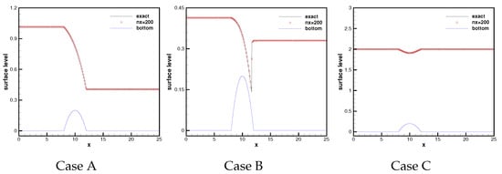
Figure 3.
Surface level at .
4.1.6. The Dam Break Problem over a Step
Here, we consider a dam break example over different steps.
- Case AFurther, we implement an example from [45] with the below initial dataand over a step-like bottomOver time, this example produces a rarefaction moving to the left and a shock moving to the right.
- Case BThe initial conditions areover the same bottom (above). Over time, this example develops two shocks moving in different directions.
- Case CThis example is from [9] and the initial data areover a step bottom
- Case DThe initial data areover the same bottom of Case C.
Figure 4 presents the numerical results at on the same mesh with 200 cells against the exact ones, and good agreement is clearly achieved. Moreover, all numerical results are free of spurious numerical ossications and maintain steep discontinuous transitions at the same time.
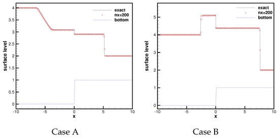
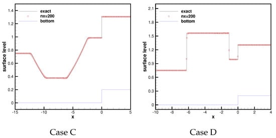
Figure 4.
Surface level at .
4.2. 2D System
In the following, we deal with the 2D examples.
4.2.1. WB Property Test
Firstly, we borrow a numerical example from [38] to confirm the WB property and use the below initial data
with as the bottom.
Table 5 shows the errors on a mesh with cells at . Clearly, all the errors are the same as the machine accuracy; this implies the successful achievement of the WB property accordingly, even for the 2D system.
Table 5.
Errors with different precisions.
4.2.2. A Small Perturbation of a 2D Steady State Flow
In the end, we deal with an example from [39]. This example has been widely used; see [38,40,42,46,47]. The initial data are
over an elliptical-like bottom on . So, the surface level is almost flat, except for , where h is perturbed upward by . Actually, the initial data can be considered to be a small perturbation to a steady state.
Figure 5 presents thirty contours of the surface level at different ending times and displays the right-going disturbance as it propagates past the hump on cells. It can be observed that small complex features are all obviously resolved by the current method and the results are comparable with those in [38,40,42,46,47].
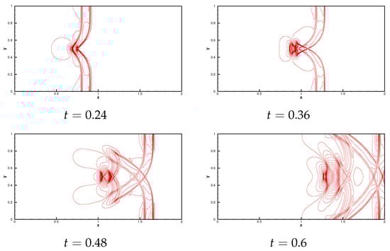
Figure 5.
The contours of surface level on a mesh with cells. Top left: at time from to ; Top right: at time from to ; Bottom left: at time from to ; Bottom right: at time from to .
5. Conclusions
In this study, we propose a new DG method according to non-conservative hyperbolic systems. The proposed method uses the one-stage ADER approach to realize the temporal discretization. To realize the high-order local time evolution, we use the DT procedure instead of the CK procedure to recursively obtain the spatiotemporal expansion coefficients using the spatial expansion coefficients. Compared with the CK procedure, the DT procedure is more concise, and the programming is more convenient. Moreover, the proposed method needs less computer storage due to the absence of intermediate stages, and is free of solving the generalized Riemann problems at inter-cells. The resulting method is an ideal candidate for parallel computing on supercomputers, thanks to the explicit one-step nature as well as the compact stencil. We can easily proceed to arbitrary high-order accuracy both in space and time without much coding effort based on the DT procedure. In conclusion, the proposed method is one-step, one-stage, and fully-discrete. In addition, we apply the proposed method to solve the one- and two-dimensional SWEs over non-flat bottom topographies. Extensive numerical results illustrate the high-order accuracy, the WB property, and the good resolutions for discontinuous solutions. In the future, we will extend this method to solve the two-layer SWEs and two-phase flow problems.
Author Contributions
Methodology, S.Q.; Software, B.W.; Writing—original draft, X.Z.; Supervision, G.L. All authors have read and agreed to the published version of the manuscript.
Funding
The author Gang Li is supported the National Natural Science Foundation of China (Grant No. 11771228) and by the Natural Science Foundation of Shandong Province (Grant No. ZR2023MA012). The author Shouguo Qian is supported by the Natural Science Foundation of Shandong Province (Grant No. ZR2021MA072).
Data Availability Statement
The original contributions presented in the study are included in the article, further inquiries can be directed to the corresponding authors.
Conflicts of Interest
The authors declare no conflicts of interest.
Appendix A
| Algorithm A1: The algorithm of the DT procedure for 1D SWEs |
|
References
- Maso, G.D.; LeFloch, P.G.; Murat, F. Definition and weak stability of nonconservative products. J. Math. Pures Appl. 1995, 74, 483–548. [Google Scholar]
- Castro, M.J.; Gallardo, J.M.; Parés, C. High-order finite volume schemes based on reconstruction of states for solving hyperbolic systems with nonconservative products. applications to shallow-water systems. Math. Comput. 2006, 75, 1103–1134. [Google Scholar] [CrossRef]
- Parés, C. Numerical methods for nonconservative hyperbolic systems: A theoretical framework. Siam J. Numer. Anal. 2006, 44, 300–321. [Google Scholar] [CrossRef]
- Toumi, I. A weak formulation of Roe’s approximate Riemann solver. J. Comput. Phys. 1992, 102, 360–373. [Google Scholar] [CrossRef]
- Dumbser, M.; Castro, M.; Parés, C.; Toro, E.F. ADER schemes on unstructured meshes for nonconservative hyperbolic systems: Applications to geophysical flows. Comput. Fluids 2009, 38, 1731–1748. [Google Scholar] [CrossRef]
- Dumbser, M.; Hidalgo, A.; Zanotti, O. High order space–time adaptive ADER-WENO finite volume schemes for non-conservative hyperbolic systems. Comput. Methods Appl. Mech. Eng. 2014, 268, 359–387. [Google Scholar] [CrossRef]
- Dumbser, M.; Hidalgo, A.; Castro, M.J.; Parés, C.; Toro, E.F. FORCE schemes on unstructured meshes II: Nonconservative hyperbolic systems. Comput. Methods Appl. Mech. Eng. 2010, 199, 625–647. [Google Scholar] [CrossRef]
- Tian, B.L.; Toro, E.F.; Castro, C.E. A path-conservative method for a five-equation model of two-phase flow with an HLLC-type Riemann solver. Comput. Fluids 2011, 46, 122–132. [Google Scholar] [CrossRef]
- Dumbser, M.; Toro, E.F. A simple extension of the Osher Riemann solver to non-conservative hyperbolic systems. J. Sci. Comput. 2011, 48, 70–88. [Google Scholar] [CrossRef]
- Castro, M.J.; Parés, C.; Puppo, G.; Russo, G. Central schemes for nonconservative hyperbolic systems. Siam J. Sci. Comput. 2012, 34, B523–B558. [Google Scholar] [CrossRef]
- Díaz, M.J.C.; Kurganov, A.; Luna, T.M. Path-conservative central-upwind schemes for nonconservative hyperbolic systems. Esaim Math. Model. Numer. Anal. 2019, 53, 959–985. [Google Scholar] [CrossRef]
- Chu, S.S.; Kurganov, A.; Na, M.Y. Fifth-order A-WENO schemes based on the path-conservative central-upwind method. J. Comput. Phys. 2022, 469, 111508. [Google Scholar] [CrossRef]
- Li, G.; Li, J.J.; Qian, S.G.; Gao, J.M. A well-balanced ADER discontinuous Galerkin method based on differential transformation procedure for shallow water equations. Appl. Math. Comput. 2021, 395, 125848. [Google Scholar] [CrossRef]
- Parés, C. Path-conservative numerical methods for nonconservative hyperbolic systems. In Numerical Methods for Balance Laws; Quaderni di Matematica; Dipto. di Matematica della Seconda Universitá di Napoli: Naples, Italy, 2014; Volume 24, pp. 67–122. [Google Scholar]
- Castro, M.J.; Asuncíon, M.; Fernández-Nieto, E.D.; Gallardo, J.M.; Vida, J.M.G.; Macías, J.; Moraies, T.; Ortega, S.; Parés, C. A review on high order well-balanced path-conservative finite volume schemes for geophysical flows. Proc. Int. Congr. Math. 2018, 4, 3533–3558. [Google Scholar]
- Ayaz, F. On the two-dimensional differential transform method. Appl. Math. Comput. 2003, 143, 361–374. [Google Scholar] [CrossRef]
- Ayaz, F. Solutions of the system of differential equations by differential transform method. Appl. Math. Comput. 2004, 147, 547–567. [Google Scholar] [CrossRef]
- Kurnaza, A.; Oturanc, G.; Kiris, M.E. n-Dimensional differential transformation method for solving PDEs. Int. J. Comput. Math. 2005, 82, 369–380. [Google Scholar] [CrossRef]
- Zhang, Y.J.; Li, G.; Qian, S.G.; Gao, J.M. A new ADER discontinuous Galerkin method based on differential transformation procedure for hyperbolic conservation laws. Comput. Appl. Math. 2021, 40, 139. [Google Scholar] [CrossRef]
- Greenberg, J.M.; Leroux, A.Y. A well-balanced scheme for the numerical processing of source terms in hyperbolic equations. Siam J. Numer. Anal. 1996, 33, 1–16. [Google Scholar] [CrossRef]
- Greenberg, J.M.; Leroux, A.Y.; Baraille, R.; Noussair, A. Analysis and approximation of conservation laws with source terms. Siam J. Numer. Anal. 1997, 34, 1980–2007. [Google Scholar] [CrossRef]
- Noelle, S.; Xing, Y.L.; Shu, C.-W. High-order well-balanced schemes. In Numerical Methods for Balance Laws; Puppo, G., Russo, G., Eds.; Quaderni di Matematica: Naples, Italy, 2010. [Google Scholar]
- Dumbser, M.; Munz, C.D. ADER discontinuous Galerkin schemes for aeroacoustics. Comput. Rendus Mec. 2005, 333, 683–687. [Google Scholar] [CrossRef]
- Dumbser, M. Arbitrary High Order Schemes for the Solution of Hyperbolic Conservation Laws in Complex Domains; Shaker Verlag: Aachen, Germany, 2005. [Google Scholar]
- Dumbser, M.; Munz, C.D. Arbitrary high order discontinuous Galerkin schemes. In Numerical Methods for Hyperbolic and Kinetic Problems; Cordier, S., Goudon, T., Gutnic, M., Sonnendrucker, E., Eds.; IRMA series in mathematics and theoretical physics; EMS Publishing House: Helsinki, Finland, 2005; pp. 295–333. [Google Scholar]
- Toro, E.F.; Millington, R.C.; Nejad, L.A.M. Towards very high order Godunov schemes. In Godunov Methods. Theory and Applications; Toro, E.F., Ed.; Kluwer/Plenum Academic Publishers: New York, NY, USA, 2001; pp. 905–938. [Google Scholar]
- Titarev, V.A.; Toro, E.F. ADER: Arbitrary high order Godunov approach. J. Sci. Comput. 2002, 17, 609–618. [Google Scholar] [CrossRef]
- Titarev, V.A.; Toro, E.F. ADER schemes for three-dimensional non-linear hyperbolic systems. J. Comput. Phys. 2005, 204, 715–736. [Google Scholar] [CrossRef]
- Dumbser, M.; Munz, C.D. Building blocks for arbitrary high order discontinuous Galerkin schemes. J. Sci. Comput. 2006, 27, 215–230. [Google Scholar] [CrossRef]
- Duan, J.; Tang, H. An efficient ADER discontinuous Galerkin scheme for directly solving Hamilton-Jacobi equation. J. Comput. Math. 2020, 38, 58–83. [Google Scholar]
- Dumbser, M.; Balsara, D.; Toro, E.F.; Munz, C.D. A unified framework for the construction of one-step finite-volume and discontinuous Galerkin schemes. J. Comput. Phys. 2008, 227, 8209–8253. [Google Scholar] [CrossRef]
- Pukhov, G.E. Differential transforms and circuit theory. Int. J. Circuit Theory Appl. 1982, 10, 265–276. [Google Scholar] [CrossRef]
- Zhou, J.K. Differential Transformation and Its Applications for Electrical Circuits; Huazhong University Press: Wuhan, China, 1986. [Google Scholar]
- Norman, M.R.; Finkel, H. Multi-moment ADER-Taylor methods for systems of conservation laws with source terms in one dimension. J. Comput. Phys. 2012, 231, 6622–6642. [Google Scholar] [CrossRef]
- Cockburn, B.; Shu, C.-W. The Runge–Kutta discontinuous Galerkin method for conservation laws V: Multidimensional systems. J. Comput. Phys. 1998, 141, 199–224. [Google Scholar] [CrossRef]
- Shu, C.-W. TVB uniformly high-order schemes for conservation laws. Math. Comput. 1987, 49, 105–121. [Google Scholar] [CrossRef]
- Shu, C.-W. Total-variation-diminishing time discretizations. Siam J. Sci. Stat. Comput. 1988, 9, 1073–1084. [Google Scholar] [CrossRef]
- Xing, Y.L.; Shu, C.-W. High order finite difference WENO schemes with the exact conservation property for the shallow water equations. J. Comput. Phys. 2005, 208, 206–227. [Google Scholar] [CrossRef]
- LeVeque, R.J. Balancing source terms and flux gradient on high-resolution Godunov methods: The quasi-steady wave-propagation algorithm. J. Comput. Phys. 1998, 146, 346–365. [Google Scholar] [CrossRef]
- Xing, Y.L.; Shu, C.-W. A new approach of high order well-balanced finite volume WENO schemes and discontinuous Galerkin methods for a class of hyperbolic systems with source terms. Commun. Comput. Phys. 2006, 1, 100–134. [Google Scholar]
- Vukovic, S.; Sopta, L. ENO and WENO schemes with the exact conservation property for one-dimensional shallow water equations. J. Comput. Phys. 2002, 179, 593–621. [Google Scholar] [CrossRef]
- Li, G.; Caleffi, V.; Qi, Z.K. A well-balanced finite difference WENO scheme for shallow water flow model. Appl. Math. Comput. 2015, 265, 1–16. [Google Scholar] [CrossRef][Green Version]
- Vazquez-Cendon, M.E. Improved treatment of source terms in upwind schemes for the shallow water equations in channels with irregular geometry. J. Comput. Phys. 1999, 148, 497–526. [Google Scholar] [CrossRef]
- Goutal, N.; Maurel, F. Proceedings of the Second Workshop on Dam-Break Wave Simulation; Technical Report HE-43/97/016/A; Electricite´ de France, De´partement Laboratoire National d’Hydraulique, Groupe Hydraulique Fluviale: Chatou, France, 1997. [Google Scholar]
- Alcrudo, F.; Benkhaldoun, F. Exact solutions to the Riemann problem of the shallow water equations with a bottom step. Comput. Fluids 2001, 30, 643–671. [Google Scholar] [CrossRef]
- Li, G.; Lu, C.; Qiu, J. Hybrid well-balanced WENO schemes with different indicators for shallow water equations. J. Sci. Comput. 2012, 51, 527–559. [Google Scholar] [CrossRef]
- Caleffi, V. A new well-balanced Hermite weighted essentially non-oscillatory scheme for shallow water equations. Int. J. Numer. Methods Fluids 2011, 67, 1135–1159. [Google Scholar] [CrossRef]


Disclaimer/Publisher’s Note: The statements, opinions and data contained in all publications are solely those of the individual author(s) and contributor(s) and not of MDPI and/or the editor(s). MDPI and/or the editor(s) disclaim responsibility for any injury to people or property resulting from any ideas, methods, instructions or products referred to in the content. |
© 2024 by the authors. Licensee MDPI, Basel, Switzerland. This article is an open access article distributed under the terms and conditions of the Creative Commons Attribution (CC BY) license (https://creativecommons.org/licenses/by/4.0/).