Interdisciplinary Education Promotes Scientific Research Innovation: Take the Composite Control of the Permanent Magnet Synchronous Motor as an Example

Abstract

Intersecting disciplines, as an important trend in the development of modern academic research and education, have exerted a profound and positive influence on scientific research activities. Based on control theory and fractional-order theory, this paper presents a novel approach for the speed regulation of a permanent magnet synchronous motor (PMSM) in the presence of uncertainties and external disturbances. The proposed method is a composite control based on a model-free sliding mode and a fractional-order ultra-local model. The model-free sliding mode is a control strategy that utilizes the sliding mode control methodology without explicitly relying on a mathematical model of the system being controlled. The fractional-order ultra-local model is a mathematical representation of a dynamic system that incorporates the concept of fractional-order derivatives. The core of the controller is a new type of fractional-order fast nonsingular terminal sliding mode surface, which ensures high robustness, quick convergence, while preventing singularity. Moreover, a novel fractional-order nonlinear extended state observer is proposed to estimate both internal and external disturbances of the fractional-order ultra-local model. The stability of the system is analyzed using both the Lyapunov stability theory and the Mittag–Leffler stability theory. The analysis confirms the convergence stability of the closed-loop system under the proposed control scheme. The comparison results indicate that the proposed composite control based on the fractional-order ultra-local model is a promising solution for regulating the speed of PMSMs in the presence of uncertainties and disturbances.

1. Introduction

In the modern education system, the vigorous development of interdisciplinary disciplines promotes in-depth reform and comprehensive innovation in scientific research of unprecedented strength [1,2,3,4]. This trend not only breaks through the barriers of traditional disciplines, but also promotes the integration and regeneration of the knowledge system, and provides a fertile soil for the cultivation of composite and innovative talents [5,6]. This paper takes motor control as an example to explore a new motor control theory based on the intersection of mathematics and control disciplines. The permanent magnet synchronous motor (PMSM) is widely used in various applications due to its superior qualities, including its high efficiency, reliability, and precise control [7,8,9,10]. The primary feature of the PMSM is the presence of permanent magnets on the rotor, which generate a stable magnetic field that interacts with the stator winding to produce torque. The PMSM offers exceptional efficiency, making it an ideal choice for applications that prioritize energy conservation, including electric vehicles, industrial machinery, and household appliances [11]. Moreover, the PMSM has a high power density, which allows it to provide significant torque in a compact, space-saving design, making it ideal for applications with size restrictions [12].

Recently, fractional-order models have received increasing attention due to their ability to offer a more precise representation of complex systems compared to traditional integer-order models. These models are rooted in the concept of fractional calculus, which extends the scope of traditional integer-order derivatives and integrals to encompass non-integer orders. A fractional-order model can be formulated as a differential equation featuring a fractional-order derivative or integral, where the order of the derivative or integral can be any real number, not limited to integers. This flexibility enables a more nuanced and realistic portrayal of system dynamics.

Fractional-order models have achieved notable success in diverse fields, such as construction engineering, electricity markets, and medical science [13,14,15]. These models have demonstrated superior performance in modeling systems exhibiting nonlinear behavior, memory effects, and intricate dynamics. In summary, fractional-order models provide a versatile and potent framework for modeling complex systems. Their capacity to capture non-integer order dynamics and long-range interactions renders them an invaluable tool for researchers and engineers across various disciplines. With ongoing efforts to develop advanced modeling techniques, fractional-order models are poised to play an ever-growing role in enhancing our understanding and control of complex systems. Additionally, a fractional-order modeling approach is frequently employed to characterize the dynamics of the PMSM [16,17]. This method offers a more precise representation of the motor’s behavior, in contrast to traditional integer-order models, by integrating fractional-order elements into the model. By incorporating these fractional-order elements, the model enables a deeper understanding and more accurate prediction of the motor’s response to diverse inputs, ultimately facilitating the development of enhanced control strategies and boosting operational efficiency.

In recent years, fractional-order sliding mode control (FOSMC) has garnered significant attention in the realm of control systems, owing to its superior performance and robustness compared to traditional integer-order sliding mode control [18]. FOSMC is a control strategy that seamlessly integrates the principles of fractional calculus into the sliding mode control framework, thereby enabling more precise modeling and control of intricate dynamical systems. One of the pivotal advantages of FOSMC lies in its proficiency in effectively tackling nonlinear and uncertain systems. By embedding fractional-order dynamics within the control law, FOSMC achieves faster convergence, mitigates chattering, and enhances tracking performance. Specifically, it is worth noting that FOSMC has the advantage of reduced chattering compared to the conventional sliding mode control [19]. By incorporating the concept of fractional calculus into the sliding mode control framework, FOSMC allows for a smoother transition of the system’s state towards the sliding surface. This smoother convergence not only enhances the system’s robustness but also significantly mitigates the high-frequency oscillations, commonly known as chattering, that are inherent in traditional sliding mode control.

Consequently, it is particularly well-suited for applications in power grids, quadrotors, robots, aerospace, and other high-performance systems where precise control is paramount [20,21,22,23].

One important application of FOSMC is in the field of PMSMs. The PMSM is a highly nonlinear system, with uncertainties introduced by factors such as friction, payload variations, and modeling errors [24,25,26]. Traditional control strategies often struggle to accurately control these systems, resulting in poor performance and stability issues [27,28,29]. By utilizing FOSMC, a PMSM can achieve better trajectory tracking, disturbance rejection, and robustness against uncertainties [19,30,31]. Fractional-order dynamics help to smooth out control signals, reducing chattering and improving control accuracy. This enables the PMSM to perform complex tasks with greater precision and efficiency. Overall, FOSMC has shown great potential for a wide range of applications where precise and robust control is crucial. Its ability to handle nonlinearities, uncertainties, and disturbances makes it a valuable tool for improving the performance of complex dynamical systems in various fields, including power grids, quad-rotors, robots, aerospace, and other high-performance systems where precise and robust control is essential. With continued advances in research in this area, we can expect to see even more innovative applications of FOSMC that push the boundaries of control technology.

Model-free control represents a class of algorithms that operate without an explicit mathematical model of the controlled system. Rather than relying on a predefined model, these algorithms learn directly from data and iteratively refine their control strategies using an ultra-local model [32]. This approach is particularly advantageous in complex and uncertain systems where acquiring an accurate mathematical model may be difficult or where the model fails to capture the system’s dynamics adequately.

An extended state observer (ESO) is commonly employed to estimate the states of the ultra-local model, particularly when some states are not directly measurable [33,34]. By leveraging the ultra-local model and available measurements, the ESO can predict the unmeasured states, providing an estimate that can be utilized for control purposes. A key strength of the ESO lies in its ability to accurately estimate system states even amidst disturbances, noise, and modeling errors. In [35], a fractional-order ultra-local model is introduced to formulate the original dynamic system for simplified controller design. This approach considers model complexity, uncertainties, and disturbances, incorporating non-integer behavior and memory effects to offer a more precise representation of real-world systems. Furthermore, fractional-order models offer greater flexibility in modeling complex systems with nonlinear dynamics and time-varying parameters, thereby facilitating a deeper understanding of the system’s behavior.

The existing FOSMC and ESO, which are often constructed based on integer-order ultra-local models, possess certain limitations that arise from this fundamental construction. The reliance solely on integer-order ultra-local models in designing both FOSMC and ESO introduces limitations pertaining to the inability to fully encapsulate the inherent properties of fractional-order systems, resulting in reduced robustness, accuracy, and limited applicability in real-world scenarios where fractional-order dynamics prevail. Building on the insights provided in the preceding discussion, this paper puts forth a novel approach to model-free sliding mode control for the speed regulation system of a PMSM. This control strategy is designed to effectively manage uncertainties and external disturbances that may be present in the system. Central to this approach is the development of a fractional-order ultra-local model, which provides a more accurate representation of the system dynamics.

Through comparisons with the existing studies, our contributions to this article are further emphasized:

• In contrast to the traditional integer-order ultra-local model of the PMSM, the fractional-order ultra-local model is now being employed to more precisely represent the original complex system dynamics, thereby facilitating the development of a comprehensive controller design.
• To estimate the internal and external disturbances of this model, a novel fractional-order nonlinear extended state observer (FNESO) is proposed. To date, no other researcher has proposed this innovative approach. Although a fractional-order ESO was previously introduced in [36], it was primarily focused on constructing a fractional-order linear ESO for disturbance compensation, without fully addressing the complexities inherent in the model.
• This paper introduces a novel approach to control systems design, which incorporates the Lyapunov stability theory. Specifically, we put forward a fractional-order nonsingular terminal sliding mode control method in this study. The core of the controller is based on a new type of fractional-order sliding mode, which offers several advantages including enhanced robustness, rapid convergence, reduced chattering, and the prevention of singularities.
• The stability analysis of the closed-loop system, utilizing the proposed control method, is demonstrated through the application of the Lyapunov theorem and Mittag–Leffler theory. Additionally, a comparison of results has been conducted to validate the efficiency and distinct advantages of the proposed control approach.

The organization of this paper is outlined as follows:

Section 2 provides a brief overview of the mathematical model of the PMSM. Section 3 introduces the fundamentals of fractional-order calculus. Control strategies and stability analysis are discussed in Section 4, followed by the presentation of comparison results from simulations in Section 5. Finally, Section 6 offers concluding remarks on the study.

2. Problem Description

This section provides an in-depth introduction to the essential knowledge of the mathematical model of PMSM.

The equation for the electromagnetic torque of a PMSM is initially presented in the following manner [27]:

$$T_e={\displaystyle \frac{3}{2}}{p}_n\left({\varphi }_f{i}_q\left(t\right)+(L_d-L_q)i_d\left(t\right)i_q\left(t\right)\right)$$

(1)

where $T_e$ symbolizes the electromagnetic force of rotation; ${\varphi }_f$ is the permanent magnet flux linkage; $p_n$ is the pole pairs number; $L_d$ and $L_q$ represent the inductances of the $dq-$axes; and $i_d\left(t\right)$ and $i_q\left(t\right)$ are the components of armature currents on the $dq-$axes, respectively.

For a surface-mounted PMSM, $L_d=L_q=L$ in this paper. The mathematical model of the PMSM can be expressed as specified in reference [37,38]:

$$\left\{\begin{array}{c}{T}_e-T_L=J\dot{\omega }\left(t\right)+B\omega \left(t\right)\\ T_e={\displaystyle \frac{3}{2}}{p}_n{\varphi }_f{i}_q\left(t\right)\end{array}\right.$$

(2)

$$\dot{\omega }\left(t\right)={\displaystyle \frac{3p_n{\varphi }_f}{2J}}{i}_q\left(t\right)-{\displaystyle \frac{B}{J}}\omega \left(t\right)-{\displaystyle \frac{1}{J}}{T}_L$$

(3)

where $\omega \left(t\right)$ is the actual mechanical speed; $J$, $T_L$, and $B$ are the rotational inertia, the load torque and the friction coefficient, respectively.

The main aim of this paper is to elaborate on the control objective, which can be articulated in the following manner:

$$e\left(t\right)={\omega }_r\left(t\right)-\omega \left(t\right)=0$$

(4)

where ${\omega }_r\left(t\right)$ is the reference speed; $e\left(t\right)$ is the speed error.

3. Preliminaries

This section will provide an overview of the definitions and lemmas of fractional-order calculus. It will discuss how fractional-order integration and differentiation generalize the concepts of integer-order calculus. The two most frequently utilized definitions for fractional-order are the Riemann–Liouville definition and the Caputo definition. In this paper, we will be utilizing the Riemann–Liouville type fractional-order definition for our study. The $\epsilon$th order Riemann–Liouville fractional derivative and the $u$th order Riemann–Liouville fractional integral of function $f\left(t\right)$ are given by [39,40]:

$$\left\{\begin{array}{c}\begin{array}{l}{}_{t_0}D_t^{\epsilon }f\left(t\right)={\displaystyle \frac{1}{\mathsf{\Gamma }\left(1-\epsilon \right)}}{\displaystyle \frac{d}{dt}}{\displaystyle {\int }_{t_0}^t\frac{f\left(\tau \right)}{{\left(t-\tau \right)}^{\epsilon }}}d\tau \\ {}_{t_0}D_t^{u}f\left(t\right)={\displaystyle \frac{1}{\mathsf{\Gamma }\left(u\right)}}{\displaystyle \frac{d}{dt}}{\displaystyle {\int }_{t_0}^t\frac{f\left(\tau \right)}{{\left(t-\tau \right)}^{1-u}}}d\tau \end{array}\\ \mathsf{\Gamma }\left(z\right)={\displaystyle {\int }_0^{\infty }{e}^{-\gamma }}{\gamma }^{z-1}d\gamma \end{array}\right.$$

(5)

where $R\left(z\right)>0$, and $t$ and $t_0$ represent the upper and lower bounds of the fractional derivative and integral, $0<\epsilon$, $u<0$. In the following text, ${}_{t_0}D_t^{\epsilon }$ is abbreviated as $D_t^{\epsilon }$.

The properties of fractional-order integration and differentiation are as follows [41]:

$${\displaystyle \frac{d^n}{d{t}^n}}\left(D_t^{\epsilon }f\left(t\right)\right)=D_t^{\epsilon +n}f\left(t\right)$$

(6)

$${\displaystyle \frac{d^n}{d{t}^n}}\left(D_t^{u}f\left(t\right)\right)=D_t^{u+n}f\left(t\right)$$

(7)

where n is an integer.

The fractional-order differentiation possesses the unique property of being a linear operation, allowing for increased versatility and precision in mathematical analysis [41]:

$$D_t^{\epsilon }\left(af\left(t\right)+bf\left(t\right)\right)=a{D}_t^{\epsilon }f\left(t\right)+b{D}_t^{\epsilon }f\left(t\right)$$

(8)

where $a>0$ and $b>0$.

Remark 1. 

Fractional-order theory has significant advantages and broad application prospects in practical engineering applications. By introducing fractional-order calculus, a more accurate system model can be established, control accuracy and stability can be improved, and the application fields can be broadened. Therefore, it is of great significance to conduct in-depth research on fractional-order theory and its application in practical engineering.

Lemma 1 

([42,43,44]). Consider $x=0$ as the equilibrium point of the fractional-order system, and let $V\left(x,t\right)$ be a continuously differentiable function. In order for the Lyapunov function $V\left(x,t\right)$ to be valid, it must satisfy two conditions:

$$a_1‖x‖\le V\left(x,t\right)\le a_2{‖x‖}^{ab}$$

(9)

and

$$D^{\epsilon }V\left(x,t\right)\le -a_3{‖x‖}^{ab}$$

(10)

where $a_1>0$ , $a_2>0$ , $a_3>0$ , $a$ and $b$ are positive constants, and so the fractional-order system exhibits Mittag–Leffler stability.

Lemma 2 

([42,43,44]). At each passing moment, the subsequent inequality remains true.

$${D_t}^{\epsilon }\left({\displaystyle \frac{1}{2}}{\mathrm{x}}^{T}Q\mathrm{x}\right)\le {\mathrm{x}}^{T}Q{D}_t^{\epsilon }\mathrm{x}$$

(11)

where $Q\in R^{n\times n}$ is a symmetric positive-definite matrix of gains.

Remark 2. 

Due to the richer dynamic characteristics exhibited by fractional-order systems, they offer greater flexibility in system design. By incorporating the Mittag–Leffler stability criterion, engineers can devise control systems with superior performance indices while ensuring the stability of the system is maintained.

4. Control Strategies and Stability Analysis

For an unidentified nonlinear model, the notion of control without a predetermined model is described in the references [45,46]. This approach involves utilizing an ultra-local model approximation for the nonlinear system, which can be expressed as follows:

$$\dot{y}\left(t\right)=\alpha u\left(t\right)+F$$

(12)

where $\alpha$ is some given constant; $F$ represents an unknown constant parameter that potentially encompasses significant nonlinearities in the PMSM.

For any unknown nonlinear model, there is a corresponding fractional-order ultra-local model that can be effectively approximated [35]:

$$D_t^{\epsilon }y\left(t\right)=\alpha u\left(t\right)+F$$

(13)

where $D_t^{\epsilon }y\left(t\right)$ denotes the $\epsilon$-order derivative of $y\left(t\right)$.

According to Equation (13), the control input of fractional-order iPID is specifically defined as

$$u(t)={\displaystyle \frac{1}{\alpha }}\left(K_{1}e\left(t\right)+K_2\dot{e}\left(t\right)+K_3{\displaystyle \int e\left(t\right)}+D_t^{\epsilon }{y}_r\left(t\right)-\widehat{F}\right)$$

(14)

where $\widehat{F}$ represents the calculated sum of both internal and external disturbances caused by the innovative FNESO method; $y_r\left(t\right)$ is a reference output trajectory, and $e\left(t\right)=y_r\left(t\right)-y\left(t\right)$; $K_1>0$, $K_2>0$, $K_3>0$.

By substituting Equation (14) into Equation (13), we can deduce the following equation:

$$K_{1}e\left(t\right)+K_2\dot{e}\left(t\right)+K_3{\displaystyle \int e\left(t\right)}+D_t^{\epsilon }e\left(t\right)+\xi \left(t\right)=0$$

(15)

where $\xi \left(t\right)$ represents the estimated margin of error associated with the novel FNESO.

By applying the Laplace transform to Equation (15), we can derive the following:

$$K_{1}E\left(S\right)+K_{2}SE\left(S\right)+K_3{\displaystyle \frac{E\left(S\right)}{S}}+S^{\epsilon }E\left(S\right)+\xi \left(S\right)-\xi \left(0\right)=0$$

(16)

The final value theorem is commonly utilized in the calculation of steady-state error, providing a useful tool for determining the ultimate error as

$$\underset{t\to \infty }{\lim }e\left(t\right)=\underset{S\to 0}{\lim }{\displaystyle \frac{S^2\left(\xi \left(S\right)-\xi \left(0\right)\right)}{K_{1}S+K_2+K_3{S}^2+S^{\epsilon }}}$$

(17)

The rephrased version of Formula (17) is

$$\underset{t\to \infty }{\lim }e\left(t\right)=\underset{S\to 0}{\lim }{\displaystyle \frac{\xi \left(S\right)-\xi \left(0\right)}{\frac{K_1}{S}+\frac{K_2}{S^2}+K_3+S^{\epsilon -1}}}$$

(18)

According to Equation (18), we can obtain $e\left(t\right)=0$ when S approaches zero infinitesimally. Building upon the fractional ultra-local model (13), we can now present the commensurate fractional-order equation of state in the following form:

$$\left\{\begin{array}{c}{D}_t^{\epsilon }{x}_1=\alpha u\left(t\right)+x_2\\ D_t^{\epsilon }{x}_2=\phi \end{array}\right.$$

(19)

where $x_2$ represents the disturbance term $F$; $\phi$ is the fractional-order derivative of the disturbance term.

This paper utilizes the FNESO method to accurately estimate the $F$ value by incorporating the control input and output variables into the analysis. The construction of the novel FNESO unfolds in the following manner:

$$\left\{\begin{array}{c}{\widehat{e}}_1\left(t\right)=Z_{21}-x_1\\ D_t^{\epsilon }{Z}_{21}=Z_{22}-{\beta }_1{\widehat{e}}_1\left(t\right)+au\\ D_t^{\epsilon }{Z}_{22}=-{\beta }_{2}fal\left({\widehat{e}}_1\left(t\right)\right)\end{array}\right.$$

(20)

$$fal\left(e\left(t\right)\right)=\left\{\begin{array}{c}{\left|e\left(t\right)\right|}^{\widehat{\alpha }}\mathrm{sgn}\left(e\left(t\right)\right)\begin{array}{c}\hspace{1em}\left|e\left(t\right)\right|>\delta \end{array}\\ {\displaystyle \frac{e\left(t\right)}{{\delta }^{1-\widehat{\alpha }}}}\begin{array}{c}\hspace{1em}\mathrm{otherwise}\end{array}\end{array}\right.$$

(21)

where ${\beta }_1>0$, ${\beta }_2>0$.

Based on the extensive research and analysis found in references [47,48], this section aims to demonstrate and affirm the robustness and stability of the proposed FNESO.

Let

$$\left\{\begin{array}{c}{e}_1=Z_{21}-x_1\\ e_2=Z_{22}-x_2\end{array}\right.$$

(22)

where $e_1$ is the estimated error of $x_1$, and $e_2$ is the estimated error of $x_2$.

The fractional-order derivative given in Equation (22) is expressed as

$$\left\{\begin{array}{c}{D}_t^{\epsilon }{e}_1=e_2-{\beta }_1{e}_1\\ D_t^{\epsilon }{e}_2=-{\beta }_{2}fal\left(e_1\right)-\phi \end{array}\right.$$

(23)

Define

$$\left\{\begin{array}{c}{e}_1^{\prime }=e_1\\ e_2^{\prime }=e_2-{\beta }_1{e}_1\end{array}\right.$$

(24)

The fractional-order derivative of Equation (24) is expressed as

$$\left\{\begin{array}{c}{D}_t^{\epsilon }{e}_1^{\prime }=e_2^{\prime }\\ D_t^{\epsilon }{e}_2^{\prime }=-{\beta }_1{e}_2^{\prime }-{\beta }_{2}fal\left(e_1\right)-\phi \end{array}\right.$$

(25)

Constructing a Lyapunov function involves selecting a function that satisfies the following criteria:

$$V={\displaystyle \underset{0}{\overset{e_1^{\prime }}{\int }}2{\beta }_{2}fal\left(\tau \right)d\tau +}{e_2^{\prime }}^2$$

(26)

In accordance with the mean value theorem for integrals, there exists a ‘$\vartheta$’ that meets the requirements of the following equation:

$$V=2{\beta }_{2}fal\left(\vartheta \right)e_1^{\prime }+{e_2^{\prime }}^T{e}_2^{\prime },\vartheta \in \left[\begin{array}{cc}0,& e_1^{\prime }\end{array}\right]$$

(27)

According to (27), we can obtain $V>0$. Next, the fractional-order derivative of Equation (27) can be expressed as follows:

$$D_t^{\epsilon }V=2{\beta }_{2}fal\left(\vartheta \right)e_2^{\prime }+D_t^{\epsilon }{e_2^{\prime }}^T{e}_2^{\prime }$$

(28)

According to Lemma 2, by substituting Equation (25) into Equation (28), we can derive the following:

$$\begin{array}{l}{D}_t^{\epsilon }V\le 2{\beta }_{2}fal\left(\vartheta \right)e_2^{\prime }+2{e_2^{\prime }}^T{D}_t^{\epsilon }{e}_2^{\prime }\\ =2{\beta }_{2}fal\left(\vartheta \right)e_2^{\prime }+2{e_2^{\prime }}^T\left(-{\beta }_1{e}_2^{\prime }-{\beta }_{2}fal\left(e_1\right)-\phi \right)\\ =2e_2^{\prime }\left(-{\beta }_1{e}_2^{\prime }-\phi +\Re \right)\end{array}$$

(29)

where $\Re ={\beta }_{2}fal\left(\vartheta \right)-{\beta }_{2}fal\left(e_1\right)$ and ${e_2^{\prime }}^T=e_2^{\prime }$.

According to (21) and (27), we can obtain $\left|\Re \right|<\mathsf{\Phi }$; $\mathsf{\Phi }$ is a positive real number.

Assumption 1 .

The gain  $\phi$  is set such that inequality is satisfied as follows: if  $\phi >\Re$ , $\left|e_2^{\prime }\right|>{\displaystyle \frac{\phi -\Re }{{\beta }_1}}$  is satisfied; if $\phi <\Re$, $\left|e_2^{\prime }\right|>-{\displaystyle \frac{\phi -\Re }{{\beta }_1}}$is satisfied.

Based on Assumption 1, it can be stated that the derivative of Equation (29) is determined as

$$D_t^{\epsilon }V<-2\left|e_2^{\prime }\left({\beta }_1{e}_2^{\prime }+\phi -\Re \right)\right|<0$$

(30)

Utilizing Lemma 1 in order to obtain Equation (30) suggests that the system’s stability is demonstrated through the Mittag–Leffler theorem.

The fractional-order sliding mode control component is incorporated as an additional input to the system to offset any estimation error and measurement noise. This additional input, denoted as $u^{\prime }\left(t\right)$, enhances the final model-free fast nonsingular terminal sliding mode controller (MFFNTSMC), which is defined as follows:

$$u\left(t\right)={\displaystyle \frac{1}{\alpha }}\left(K_{1}e\left(t\right)+K_2\dot{e}\left(t\right)+K_3{\displaystyle \int e\left(t\right)}+D_t^{\epsilon }{y}_r\left(t\right)-\widehat{F}\right)+u^{\prime }\left(t\right)$$

(31)

After substituting Equation (31) into Equation (10), the newly defined closed-loop error is as follows:

$$K_{1}e\left(t\right)+K_2\dot{e}\left(t\right)+K_3{\displaystyle \int e\left(t\right)}+D_t^{\epsilon }e\left(t\right)+\tilde{F}+\alpha u^{\prime }\left(t\right)=0$$

(32)

Hence, the additional input $u^{\prime }(t)$ is specifically aimed at offsetting the disturbance. According to the sliding mode control framework, a distinct switching function $s_1(t)$ is defined as the fractional-order fast nonsingular terminal sliding mode surface in the following way:

$$s_1\left(t\right)=D_t^{\epsilon -1}e\left(t\right)+{\lambda }_1{\left(e\left(t\right)\right)}^{p/q}+{\lambda }_2{\displaystyle \iint e\left(t\right)}+{\lambda }_3{\displaystyle \int e\left(t\right)}+{\lambda }_{4}e\left(t\right)$$

(33)

where ${\lambda }_1>0$, ${\lambda }_2>0$, ${\lambda }_3>0$, ${\lambda }_4>0$.

The derivative of Equation (33) can be calculated as follows:

$${\dot{s}}_1\left(t\right)=D_t^{\epsilon }e\left(t\right)+{\displaystyle \frac{{\lambda }_{1}p}{q}}{\left(e\left(t\right)\right)}^{\left(p/q\right)-1}+{\lambda }_2{\displaystyle \int e\left(t\right)}+{\lambda }_{3}e\left(t\right)+{\lambda }_4\dot{e}\left(t\right)$$

(34)

Then, the decision is made to implement the following reaching law:

$${\dot{s}}_1(t)=-\eta sign\left(s_1\left(t\right)\right)$$

(35)

where $\eta >0$.

Referring to the studies by (34) and (35) as well as the fractional-order ultra-local model (13), we can derive the following conclusions:

$$-K_{1}e\left(t\right)-K_2\dot{e}\left(t\right)-K_3{\displaystyle \int e\left(t\right)}-\tilde{F}-\alpha u^{\prime }(t)+{\displaystyle \frac{{\lambda }_{1}p}{q}}{\left(e(t)\right)}^{\left(p/q\right)-1}+{\lambda }_2{\displaystyle \int e\left(t\right)}+{\lambda }_{3}e\left(t\right)+{\lambda }_4\dot{e}\left(t\right)=-\eta sign\left(s_1\left(t\right)\right)$$

(36)

From Equation (36), the input $u^{\prime }\left(t\right)$ is defined as:

$$u^{\prime }\left(t\right)={\displaystyle \frac{1}{\alpha }}\left(\eta sign\left(s_1\left(t\right)\right)-K_{1}e\left(t\right)-K_2\dot{e}\left(t\right)-K_3{\displaystyle \int e\left(t\right)}-\tilde{F}+{\displaystyle \frac{{\lambda }_{1}p}{q}}{\left(e(t)\right)}^{\left(p/q\right)-1}+{\lambda }_2{\displaystyle \int e\left(t\right)}+{\lambda }_{3}e\left(t\right)+{\lambda }_4\dot{e}\left(t\right)\right)$$

(37)

Upon substituting Equation (37) into Equation (31), the total input can be rephrased in the following manner:

$$u\left(t\right)={\displaystyle \frac{1}{\alpha }}\left(D_t^{\epsilon }{y}_r\left(t\right)+\eta sign\left(s_1\left(t\right)\right)-\widehat{F}-{\tilde{F}}_{\max }+{\displaystyle \frac{{\lambda }_{1}p}{q}}{\left(e\left(t\right)\right)}^{\left(p/q\right)-1}+{\lambda }_2{\displaystyle \int e\left(t\right)}+{\lambda }_{3}e\left(t\right)+{\lambda }_4\dot{e}\left(t\right)\right)$$

(38)

Remark 3. 

The integration of the fast nonsingular terminal sliding mode surface into FOSMC provides a powerful tool for designing controllers that exhibit reduced chattering, faster convergence with finite-time stability, improved robustness, and greater flexibility in design.

Building upon the research of previous scholars [49,50], this article delves into a thorough analysis of the stability of the control strategy as highlighted in the subsequent sections. According to the Lyapunov stability theory, we introduce the Lyapunov function, defined as follows:

$$V={\displaystyle \frac{1}{2}}{s_1}^2\left(t\right)$$

(39)

Differentiating Equation (39) with respect to time yields

$$\begin{array}{l}\dot{V}=s_1\left(t\right){\dot{s}}_1\left(t\right)\\ =s_1\left(t\right)\left(D_t^{\epsilon }e\left(t\right)+{\displaystyle \frac{{\lambda }_{1}p}{q}}{\left(e\left(t\right)\right)}^{\left(p/q\right)-1}+{\lambda }_2{\displaystyle \int e\left(t\right)}+{\lambda }_{3}e\left(t\right)+{\lambda }_4\dot{e}\left(t\right)\right)\end{array}$$

(40)

Based on the findings of (34) and (35), it can be concluded that

$$D_t^{\epsilon }y\left(t\right)=D_t^{\epsilon }{y}_r\left(t\right)+\eta sign\left(s_1\left(t\right)\right)-{\tilde{F}}_{\max }+\tilde{F}+{\displaystyle \frac{{\lambda }_{1}p}{q}}{\left(e\left(t\right)\right)}^{\left(p/q\right)-1}+{\lambda }_2{\displaystyle \int e\left(t\right)}+{\lambda }_{3}e\left(t\right)+{\lambda }_4\dot{e}\left(t\right)$$

(41)

Equation (41) can be further transformed into the following expression:

$$-\eta sign\left(s_1\left(t\right)\right)+{\tilde{F}}_{\max }-\tilde{F}+{\displaystyle \frac{{\lambda }_{1}p}{q}}{\left(e\left(t\right)\right)}^{\left(p/q\right)-1}+{\lambda }_2{\displaystyle \int e\left(t\right)}+{\lambda }_{3}e\left(t\right)+{\lambda }_4\dot{e}\left(t\right)=D_t^{\epsilon }e\left(t\right)$$

(42)

By substituting Equation (42) into Equation (40), we can derive the following relationship:

$$\begin{array}{l}\dot{V}=s\left(-\eta sign\left(s\left(t\right)\right)+{\tilde{F}}_{\max }-\tilde{F}\right)\\ =-\eta \left|s\left(t\right)\right|-s\left(\tilde{F}-{\tilde{F}}_{\max }\right)\\ \le -\eta \left|s\left(t\right)\right|-\left|s\left(t\right)\right|\left|\tilde{F}-{\tilde{F}}_{\max }\right|\end{array}$$

(43)

Then, $\dot{V}$ is negative definite. Based on the Lyapunov stability theory, we can conclude that $s_1(t)$ will be bounded in finite time as $\left|s_1\left(t\right)\right|\le \mathsf{\Psi }$.

Combining $\left|s_1\left(t\right)\right|\le \mathsf{\Psi }$ with (33), we have the fractional-order nonsingular terminal sliding mode $s_1\left(t\right)$ as

$$D_t^{\epsilon -1}e\left(t\right)+{\lambda }_1{\left(e\left(t\right)\right)}^{p/q}+{\lambda }_2{\displaystyle \iint e\left(t\right)}+{\lambda }_3{\displaystyle \int e\left(t\right)+}{\lambda }_{4}e\left(t\right)-s\left(t\right)=0$$

(44)

The equation given in (44) can be expressed in a different form as:

$$\left(1-s\left(t\right){\left(D_t^{\epsilon -1}e\left(t\right)\right)}^{-1}\right)D_t^{\epsilon -1}e\left(t\right)+{\lambda }_1{\left(e\left(t\right)\right)}^{p/q}+{\lambda }_2{\displaystyle \iint e\left(t\right)}+{\lambda }_3{\displaystyle \int e\left(t\right)}+{\lambda }_{4}e\left(t\right)=0$$

(45)

When $\left(1-s\left(t\right){\left(D_t^{\epsilon -1}e\left(t\right)\right)}^{-1}\right)>0$ holds, the fractional-order nonsingular terminal sliding mode surface defined in Equation (45) will continue to be maintained as in Equation (33). Therefore, the system trajectory will continuously approach the sliding mode surface until it ultimately reaches $\left|D_t^{\epsilon -1}e\left(t\right)\right|\le \mathsf{\Psi }$.

$$D_t^{\epsilon -1}e\left(t\right)+\left({\lambda }_1-s\left(t\right){\left(e\left(t\right)\right)}^{q/p}\right){\left(e\left(t\right)\right)}^{p/q}+{\lambda }_2{\displaystyle \iint e\left(t\right)}+{\lambda }_3{\displaystyle \int e\left(t\right)}+{\lambda }_{4}e\left(t\right)=0$$

(46)

When $\left({\lambda }_1-s\left(t\right){\left(e\left(t\right)\right)}^{q/p}\right)>0$ holds, even as time passes, the fractional-order nonsingular terminal sliding mode surface as described in Equation (33) will remain unchanged. Hence, the system trajectory will continuously approach the sliding mode surface until it finally reaches ${\left(e\left(t\right)\right)}^{q/p}\le {\displaystyle \frac{\mathsf{\Psi }}{{\lambda }_1}}$.

$$D_t^{\epsilon -1}e\left(t\right)+{\lambda }_1{\left(e\left(t\right)\right)}^{p/q}+{\lambda }_2{\displaystyle \iint e\left(t\right)}+{\lambda }_{4}e\left(t\right)+\left({\lambda }_3-s\left(t\right){\left({\displaystyle \int e\left(t\right)}\right)}^{-1}\right)\left({\displaystyle \int e\left(t\right)}\right)=0$$

(47)

When $\left({\lambda }_3-s\left(t\right){\left({\displaystyle \int e\left(t\right)}\right)}^{-1}\right)>0$ is met, the fractional-order nonsingular terminal sliding mode surface will continue to be maintained as condition (47) is satisfied. Therefore, the system trajectory will continually approach the sliding mode surface until it reaches $\left|{\displaystyle \int e\left(t\right)}\right|\le {\displaystyle \frac{\mathsf{\Psi }}{{\lambda }_3}}$.

$$D_t^{\epsilon -1}e\left(t\right)+{\lambda }_1{\left(e\left(t\right)\right)}^{p/q}+\left({\lambda }_2-s\left(t\right){\left({\displaystyle \iint e\left(t\right)}\right)}^{-1}\right){\displaystyle \iint e\left(t\right)}+{\lambda }_{4}e\left(t\right)+{\lambda }_3{\displaystyle \int e\left(t\right)}=0$$

(48)

When $\left({\lambda }_2-s\left(t\right){\left({\displaystyle \iint e\left(t\right)}\right)}^{-1}\right)>0$ holds, (48) will still remain the fractional-order nonsingular terminal sliding mode surface as in (33). Therefore, the system trajectory will persistently converge to the sliding mode surface until it reaches $\left|{\displaystyle \iint e\left(t\right)}\right|\le {\displaystyle \frac{\mathsf{\Psi }}{{\lambda }_2}}$.

$$e\left(t\right)={\left({\lambda }_4\right)}^{-1}\left(D_t^{\epsilon -1}e\left(t\right)+{\lambda }_1{\left(e\left(t\right)\right)}^{p/q}+{\lambda }_2{\displaystyle \int {\displaystyle \int e\left(t\right)}}+{\lambda }_3{\displaystyle \int e\left(t\right)}-s\left(t\right)\right)$$

(49)

Expression (49) satisfies the following inequality:

$$\left|e\left(t\right)\right|\le {\left({\lambda }_4\right)}^{-1}\left(\left|D_t^{\epsilon -1}e\left(t\right)\right|+\left|{\lambda }_1{\left(e\left(t\right)\right)}^{p/q}\right|+\left|{\lambda }_2{\displaystyle \iint e\left(t\right)}\right|+\left|{\lambda }_3{\displaystyle \int e\left(t\right)}\right|+\left|s\left(t\right)\right|\right)$$

(50)

Based on the previous analysis, it can be concluded that

$$\left|e\left(t\right)\right|\le 5{\left({\lambda }_4\right)}^{-1}\mathsf{\Psi }$$

(51)

Lastly, the stability of the closed-loop control system has been demonstrated, ensuring that the control errors will be limited as indicated in Equation (51).

In this paper, we utilize the FNESO method to estimate the value of the disturbance term $F$. By substituting FNESO (20) into Equation (38), the total input can be recalculated as follows:

$$u\left(t\right)={\displaystyle \frac{1}{\alpha }}\left(D_t^{\epsilon }{y}_r\left(t\right)+\eta sign\left(s_1\left(t\right)\right)-Z_{22}+{\displaystyle \frac{{\lambda }_{1}p}{q}}{\left(e\left(t\right)\right)}^{\left(p/q\right)-1}+{\lambda }_2{\displaystyle \int e\left(t\right)}+{\lambda }_{3}e\left(t\right)+{\lambda }_4\dot{e}\left(t\right)\right)$$

(52)

The following introduces several existing model-free control algorithms, and in the next section, a comparative analysis will be conducted between existing control algorithms and the control method proposed in this paper.

The control input of iPID is clearly outlined and defined in reference [46]:

$$u\left(t\right)={\displaystyle \frac{1}{\alpha }}\left(K_{1}e\left(t\right)+K_2\dot{e}\left(t\right)+K_3{\displaystyle \int e\left(t\right)}+{\dot{y}}_r\left(t\right)-\widehat{F}\right)$$

(53)

In references [33,51], the existing control method, known as the model-free fractional-order sliding mode controller (MFFSMC), is introduced, and the design rationale for this control method is outlined as follows:

$$u\left(t\right)={\displaystyle \frac{1}{\alpha }}\left(K_{1}e\left(t\right)+K_2\dot{e}\left(t\right)+K_3{\displaystyle \int e\left(t\right)}+{\dot{y}}_r\left(t\right)-\widehat{F}\right)+u^{\prime }\left(t\right)$$

(54)

where

$$u^{\prime }\left(t\right)={\displaystyle \frac{1}{\alpha }}\left(\begin{array}{l}-K_{1}e\left(t\right)-K_2\dot{e}\left(t\right)-K_3{\displaystyle \int e\left(t\right)}+k{D}^{\epsilon }{\left|e\left(t\right)\right|}^{\alpha }\mathrm{sgn}\left(e\left(t\right)\right)\\ +{\eta }_1{s}_2\left(t\right)+{\eta }_2{\left|s_2\left(t\right)\right|}^{\alpha }\mathrm{sgn}\left(s_2\left(t\right)\right)-F\end{array}\right)$$

(55)

Based on the principles of sliding mode control, a switching function $s_2(t)$ is introduced to define the fractional-order nonsingular terminal sliding mode as follows:

$$s_2\left(t\right)=e\left(t\right)+k{D}^{\epsilon -1}{\left|e\left(t\right)\right|}^{\alpha }\mathrm{sgn}\left(e\left(t\right)\right)$$

(56)

After substituting Equation (56) into Equation (54), the overall input can be reformulated as follows:

$$u\left(t\right)={\displaystyle \frac{1}{\alpha }}\left({\dot{y}}_r\left(t\right)-\widehat{F}-F_{\max }+k{D}^{\epsilon }{\left|e\left(t\right)\right|}^{\alpha }\mathrm{sgn}\left(e\left(t\right)\right)+{\eta }_{1}s+{\eta }_2{\left|s\right|}^{\alpha }\mathrm{sgn}\left(s\right)\right)$$

(57)

The current control method uses a traditional ESO to estimate the total disturbance. The traditional ESO equation is as follows:

$$\left\{\begin{array}{c}{\widehat{e}}_1\left(t\right)=Z_{21}-x_1\\ {\dot{Z}}_{21}=Z_{22}-{\beta }_{1}fal\left({\widehat{e}}_1\left(t\right)\right)+au\\ {\dot{Z}}_{22}=-{\beta }_{2}fal\left({\widehat{e}}_1\left(t\right)\right)\end{array}\right.$$

(58)

Figure 1 depicts an innovative field-oriented control system designed for regulating the speed of a PMSM, which is based on the innovative MFFNTSMC technique integrated with FNESO.

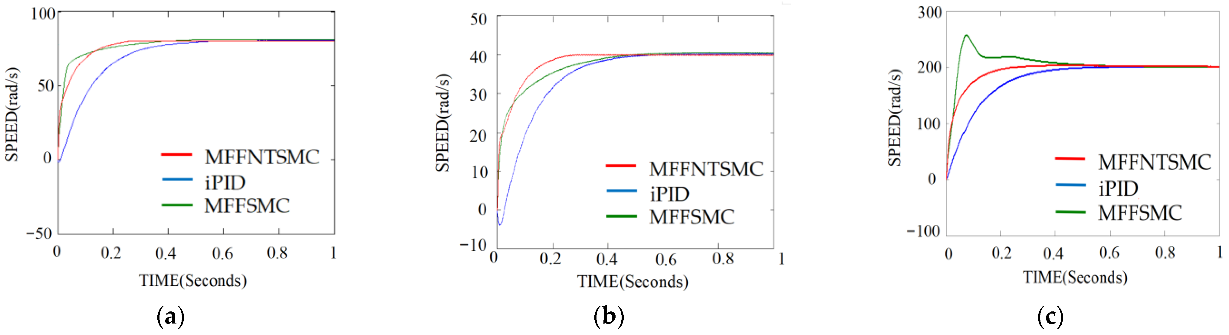
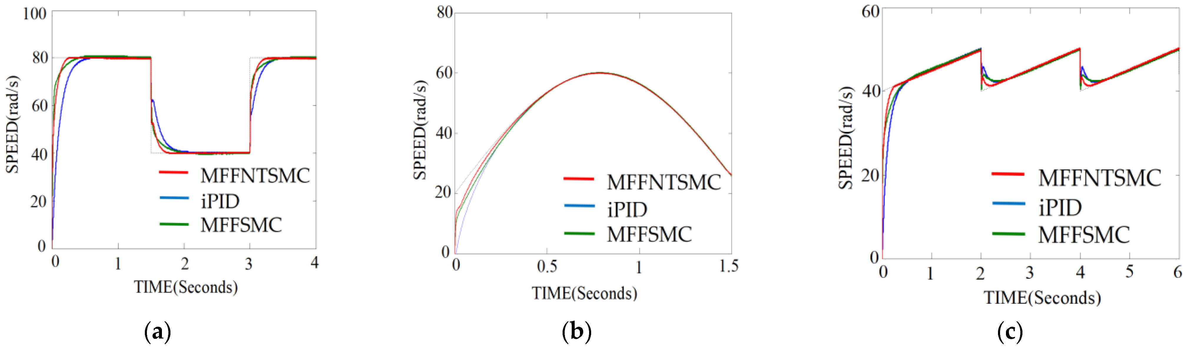
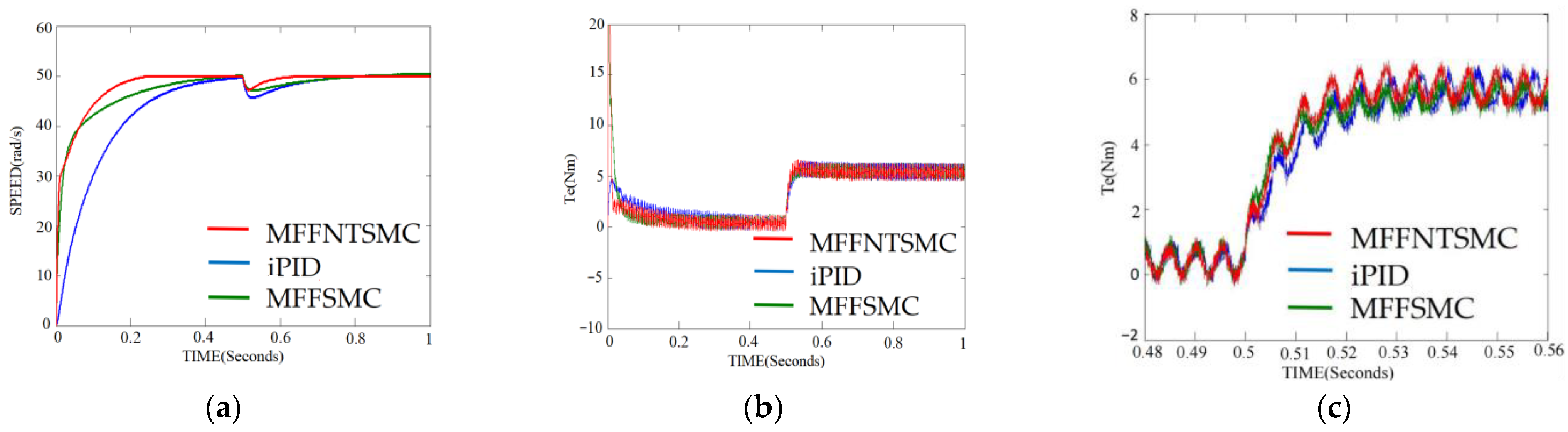
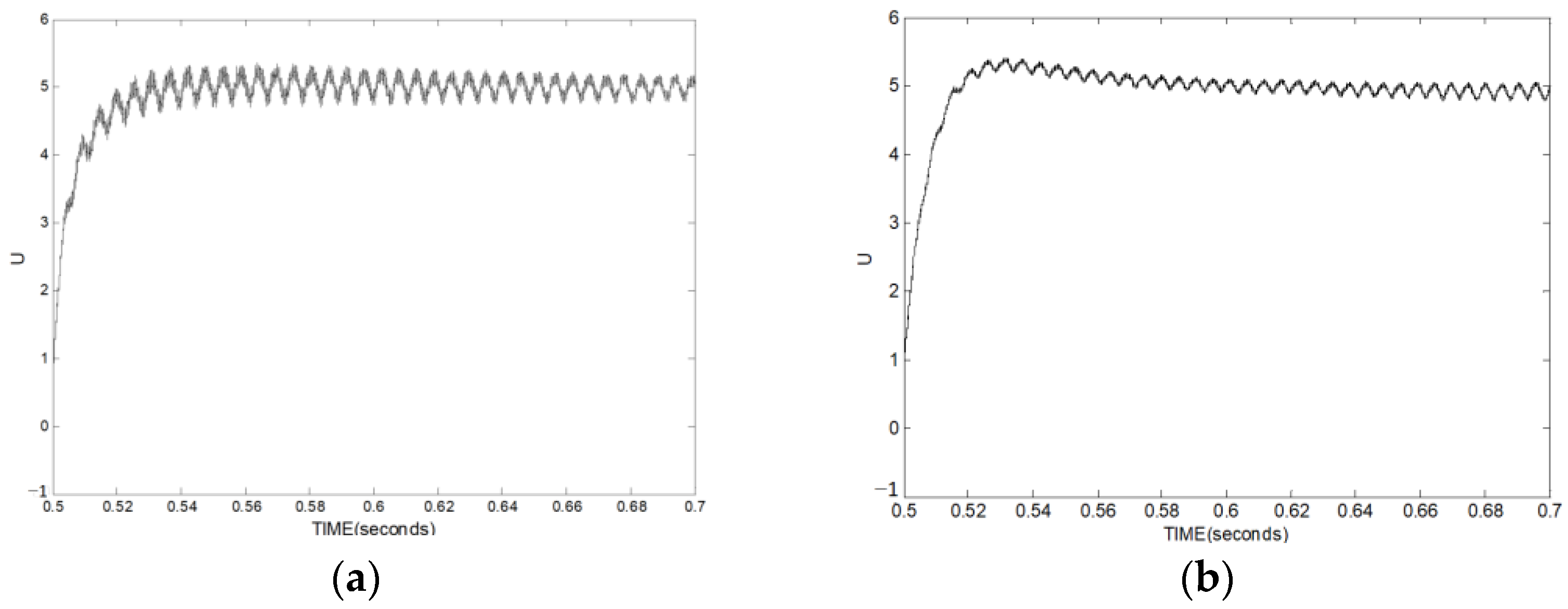
5. Comparative Results

In this section, we present comparative results to verify the speed regulation performance of the proposed MFFNTSMC. To demonstrate the effectiveness of our approach, we established a PMSM speed regulation system using field-oriented control with various control strategies in Matlab (https://www.mathworks.com/products/matlab.html, accessed on 1 August 2024). We compared our proposed control strategy with the traditional iPID and traditional MFFSMC methods. During the comparative simulations, all three current loops were controlled using PI controllers with identical parameters. Furthermore, to better highlight the advantages of our proposed control strategy, we ensured that certain parameters in the different control strategies remained consistent, thereby minimizing the impact of parameter variations on the comparison results. The control parameters for the iPID in the speed loop are specified as follows: $\alpha =100$, $K_1=10$, $K_2=0.1$, $K_3=0.5$, ${\beta }_1=2000$, and ${\beta }_2=\mathrm{150,000}$. The specified control parameters of the conventional MFFSMC in the speed loop are as follows: $\alpha =100$, $\alpha =0.5$, $\epsilon =0.9$, $k=0.5$, ${\eta }_1=5$, ${\eta }_2=0.5$, ${\beta }_1=2000$, and ${\beta }_2=\mathrm{150,000}$. The control parameters in the speed loop of the proposed MFFNTSMC system are presented as follows: $\alpha =100$, $p=3$, $\epsilon =0.9$, $k=0.5$, ${\lambda }_1=5$, ${\lambda }_2=0.5$, ${\beta }_1=\mathrm{20,000}$, ${\beta }_2=\mathrm{300,000}$, $q=5$, ${\lambda }_3=50$, ${\lambda }_4=0.1$, and $\eta =2$. This paper has referred to the motor parameters presented in papers [52] and [53].

Table 1. Key parameters of the PMSM.

$\mathit{L}$	${\mathit{\varphi }}_{\mathit{f}}$	$\mathit{J}$	$\mathit{B}$	${\mathit{p}}_{\mathit{n}}$	${\mathit{R}}_{\mathit{s}}$
$5.25\mathrm{mH}$	$0.1827 \mathrm{Wb}$	$0.009 \mathrm{kg}·{\mathrm{m}}^2$	$0.008 \mathrm{N}·\mathrm{m}·\mathrm{s}/\mathrm{r}\mathrm{a}\mathrm{d}$	4	0.958 $\mathsf{\Omega }$

provides a comprehensive overview of the essential parameters associated with the PMSM.

• Case I: speed response curves comparison.

In this case study, we will be comparing the speed response curves of different systems. By analyzing the data collected from these curves, we will be able to determine which system performs most efficiently in terms of speed response. Through this comparison, we aim to identify the strengths and weaknesses of each system, providing valuable insights to inform decision-making and optimize performance. The speed response of the PMSM under the proposed and conventional existing controllers is compared in Figure 2 and Figure 3. To evaluate the control performance of different controllers, the reference speed is set at 80 rad/s, 40 rad/s, and 200 rad/s. Figure 2 illustrates the speed response curves under the iPID, MFFSMC, and MFFNTSMC methods for various step signals without load. Meanwhile, Figure 3 showcases the speed response curves under the same methods for different step signals with $5 \mathrm{N}·\mathrm{m}$ load. The results depicted in Figure 2 and Figure 3 demonstrate that the reaching time achieved with the proposed MFFNTSMC algorithm is significantly shorter compared to that of the conventional existing controller. These figures vividly illustrate how the dynamic system closely follows the reference speed with much greater speed and precision when utilizing the MFFNTSMC algorithm as opposed to the conventional controller. These findings unequivocally showcase the superior dynamic characteristics of the proposed MFFNTSMC algorithm.

• Case II: comparison of speed-tracking performance.

To demonstrate the remarkable speed-tracking capabilities of both traditional composite control and the newly proposed composite control methods, a comparison of the tracking abilities of a sine wave signal, square wave signal, and triangular wave signal under different controllers is made. The outcomes of this test can be seen in Figure 4 and Figure 5. The comparison of tracking curves is shown in Figure 4, and the tracking error is shown in Figure 5. The thorough examinations reveal that the tracking error for the reference is significantly reduced in the proposed composite control method as compared to the conventional composite control method.

• Case III: comparing resistance to uncertainties and disturbances.

The system uncertainties and disturbances in this paper are primarily caused by sudden changes in the external load of the PMSM. To assess the robustness of the proposed MFFNTSMC method, a sudden change in external load was introduced during the simulation. The reference speed was set at 50 rad/s and the simulation time at 1 s. In Figure 6, the external load increased from 0 $\mathrm{N}·\mathrm{m}$ to 5 $\mathrm{N}·\mathrm{m}$ at 0.5 s under the iPID, MFFSMC, and MFFNTSMC methods, respectively. In Figure 7, the external load decreased from 5 $\mathrm{N}·\mathrm{m}$ to 0 $\mathrm{N}·\mathrm{m}$ at 0.5 s under the same control methods. Figure 6 and Figure 7 illustrate how external load disturbances impact the control strategies. Remarkably, the recovery time under the MFFNTSMC method was found to be significantly shorter than that under the iPID and MFFSMC methods, indicating the superior robustness of the proposed MFFNTSMC compared to traditional control methods.

• Case IV: comparison of disturbance estimation.

The comparison of disturbance estimation between the proposed FNESO and conventional ESO can be seen in Figure 8. In Figure 8a, observations from different observers on the same disturbance are depicted. Figure 8b,c showcase the error in disturbance estimation. The blue curves represent the disturbance in the control system when using the conventional ESO, while the red curves represent the proposed FNESO. The accuracy of the proposed FNESO is superior to that of the conventional ESO when operating under the same conditions. The analysis further demonstrates that the FNESO is convergent and effectively tracks the system’s state variables, confirming the efficacy of this estimation method.

• Case V: comparison of control signals.

A comparison of the simulation results of control signals provides valuable insights into the performance and effectiveness of different control methodologies. Figure 9 shows the comparison of control signals between the proposed MFFNTSMC and MFFSMC when the external load changes from 0 $\mathrm{N}·\mathrm{m}$ to 5 $\mathrm{N}·\mathrm{m}$ at 0.5 s. Figure 10 shows the comparison of control signals between the proposed MFFNTSMC and MFFSMC when the external load changes from 5 $\mathrm{N}·\mathrm{m}$ to 0 $\mathrm{N}·\mathrm{m}$ at 0.5 s. From Figure 9 and Figure 10, it is clear that the control signals of the controller proposed in this paper exhibit less chattering and a shorter response time.

6. Conclusions

Based on the foundations of mathematics and control theory, this study introduces an innovative control strategy for the PMSM speed regulation system, utilizing the novel FNESO and the proposed MFFNTSMC. A new sliding surface, referred to as the fractional-order fast nonsingular terminal sliding mode surface has been devised to enhance robustness and improve dynamic response. Moreover, a recently developed FNESO is employed to estimate uncertain terms within the PMSM speed regulation system. Through comparative simulations, it has been conclusively shown that the proposed strategy exhibits excellent speed-tracking performance and robustness. The integration of FNESO and MFFNTSMC has been found to be highly effective in achieving superior control outcomes for PMSM speed regulation. This novel approach offers substantial advancements in control strategies for PMSM systems, providing enhanced performance and stability in speed regulation.

The proposed composite control presents a promising direction for future research, with opportunities to explore experimental validation, extension to MIMO systems, the optimization of control parameters, combinations with other advanced control strategies, and applications to specific industrial systems.

References

1. Li, Y.; Yan, Y.; Li, M.J. Does interdisciplinary research lead to higher faculty performance? Evidence from an accelerated research university in China. Sustainability 2022, 14, 13977. [Google Scholar] [CrossRef]
2. John, H. Sustaining interdisciplinary education: Developing boundary crossing governance. High. Educ. Res. Dev. 2018, 37, 1424–1438. [Google Scholar]
3. John, G.H.; Stephanie, S.; Alison, F.S.; Amal, D.A.; Michael, J.A.; Ayaz, A.; Dik, B.; John, V.B.; David, B.; Adam, B.; et al. Potential for chemistry in multidisciplinary, interdisciplinary, and transdisciplinary teaching activities in higher education. J. Chem. Educ. 2021, 98, 1124–1145. [Google Scholar]
4. Sandra, B.; ElSayary, A. Driving transformation in higher education: Exploring the process and impact of educational innovations for sustainability through interdisciplinary studies. High. Educ. Q. 2024, e12529. [Google Scholar] [CrossRef]
5. Van den Beemt, A.; MacLeod, M.; Van der Veen, J.; Van de Ven, A.; Van Baalen, S.; Klaassen, R.; Boon, M. Interdisciplinary engineering education: A review of vision, teaching, and support. J. Eng. Educ. 2020, 109, 508–555. [Google Scholar] [CrossRef]
6. Turner, R.; Cotton, D.; Morrison, D.; Kneale, P. Embedding interdisciplinary learning into the first-year undergraduate curriculum: Drivers and barriers in a cross-institutional enhancement project. Teach. High. Educ. 2024, 29, 1092–1108. [Google Scholar] [CrossRef]
7. Xie, F.; Xu, J.; Shen, M.; Zheng, Z. Current harmonic suppression strategy for permanent magnet synchronous motor based on small phase angle resonant controller. IET Electr. Power Appl. 2024, 8, 556–564. [Google Scholar] [CrossRef]
8. Zhao, K.; Liu, W.; Zhou, R.; Dai, W.; Wu, S.; Qiu, P.; Yin, Y.; Jia, N.; Yi, J.; Huang, G. Model-free fast integral terminal sliding-mode control method based on improved fast terminal sliding-mode observer for PMSM with unknown disturbances. ISA Trans. 2023, 143, 572–581. [Google Scholar] [CrossRef]
9. Wang, S.; Gan, H.; Luo, Y.; Luo, X.; Chen, Y. A Fractional-order ADRC architecture for a PMSM position servo system with improved disturbance rejection. Fractal Fract. 2024, 8, 54. [Google Scholar] [CrossRef]
10. Xiong, J.; Fu, X. Extended two-state observer-based speed control for PMSM with uncertainties of control input gain and lumped disturbance. IEEE Trans. Ind. Electron. 2024, 71, 6172–6182. [Google Scholar] [CrossRef]
11. Gao, P.; Zhang, G.; Ouyang, H.; Mei, L. An adaptive super twisting nonlinear Fractional-order PID sliding mode control of permanent magnet synchronous motor speed regulation system based on extended state observer. IEEE Access 2020, 8, 53498–53510. [Google Scholar] [CrossRef]
12. Gao, P.; Pan, H. Model-free double Fractional-order integral sliding mode control for permanent magnet synchronous motor based electric mopeds drive system. IEICE Electron. Express 2023, 20, 20230178. [Google Scholar] [CrossRef]
13. Abbes, A.; Ouannas, A.; Shawagfeh, N.; Jahanshahi, H. The Fractional-order discrete COVID-19 pandemic model: Stability and chaos. Nonlinear Dyn. 2023, 111, 965–983. [Google Scholar] [CrossRef] [PubMed]
14. Dassios, I.; Kërçi, T.; Baleanu, D.; Milano, F. Fractional-order dynamical model for electricity markets. Math. Methods Appl. Sci. 2023, 46, 8349–8361. [Google Scholar] [CrossRef]
15. Zheng, Z.; Cai, Z.; Su, G.; Huang, S.; Wang, W.; Zhang, Q.; Wang, Y. A new Fractional-order model for time-dependent damage of rock under true triaxial stresses. Int. J. Damage Mech. 2023, 32, 50–72. [Google Scholar] [CrossRef]
16. Xue, W.; Li, Y.; Cang, S.; Jia, H.; Wang, Z. Chaotic behavior and circuit implementation of a Fractional-order permanent magnet synchronous motor model. J. Frankl. Inst. 2015, 352, 2887–2898. [Google Scholar] [CrossRef]
17. Zhang, S.; Wang, C.; Zhang, H.; Ma, P.; Li, X. Dynamic analysis and bursting oscillation control of Fractional-order permanent magnet synchronous motor system. Chaos Solitons Fractals 2022, 156, 111809. [Google Scholar] [CrossRef]
18. Sheng, Y.; Gan, J.; Guo, X. Predefined-time Fractional-order time-varying sliding mode control for arbitrary order systems with uncertain disturbances. ISA Trans. 2024, 146, 236–248. [Google Scholar] [CrossRef]
19. Zhang, B.; Pi, Y.; Luo, Y. Fractional-order sliding-mode control based on parameters auto-tuning for velocity control of permanent magnet synchronous motor. ISA Trans. 2012, 51, 649–656. [Google Scholar] [CrossRef]
20. Chu, Y.; Hou, S.; Wang, C.; Fei, J. Recurrent-neural-network-based Fractional-order sliding mode control for harmonic suppression of power grid. IEEE Trans. Ind. Inform. 2023, 19, 9979–9990. [Google Scholar] [CrossRef]
21. El Ferik, S.; Al-Qahtani, F.M.; Saif, A.W.A.; Al-Dhaifallah, M. Robust FOSMC of quadrotor in the presence of slung load. ISA Trans. 2023, 139, 106–121. [Google Scholar] [CrossRef]
22. Chávez-Vázquez, S.; Lavín-Delgado, J.E.; Gómez-Aguilar, J.F.; Razo-Hernández, J.R.; Etemad, S.; Rezapour, S. Trajectory tracking of Stanford robot manipulator by Fractional-order sliding mode control. Appl. Math. Model. 2023, 120, 436–462. [Google Scholar] [CrossRef]
23. Fan, J.; Chen, S.; Wang, W.; Ji, Y.; Liu, N. Piecewise trajectory and angle constraint based Fractional-order sliding mode control. IEEE Trans. Aerosp. Electron. Syst. 2023, 59, 6782–6797. [Google Scholar] [CrossRef]
24. Zhang, L.; Tao, R.; Zhang, Z.X.; Chien, Y.R.; Bai, J. PMSM non-singular fast terminal sliding mode control with disturbance compensation. Inf. Sci. 2023, 642, 119040. [Google Scholar] [CrossRef]
25. Wang, C.; Liu, F.; Xu, J.; Pan, J. A SMC-based accurate and robust load speed control method for elastic servo system. IEEE Trans. Ind. Electron. 2023, 71, 2300–2308. [Google Scholar] [CrossRef]
26. Tian, M.; Wang, B.; Yu, Y.; Dong, Q.; Xu, D. Adaptive active disturbance rejection control for uncertain current ripples suppression of PMSM Drives. IEEE Trans. Ind. Electron. 2023, 71, 2320–2331. [Google Scholar] [CrossRef]
27. Wu, J.; Zhao, Y.; Kong, Y.; Liu, Q.; Zhang, L. Hierarchical non-singular terminal sliding mode control with finite-time disturbance observer for PMSM speed regulation system. IEEE Trans. Transp. Electrif. 2023. [Google Scholar] [CrossRef]
28. Hou, Q.; Xu, S.; Zuo, Y.; Wang, H.; Sun, J.; Lee, C.H.; Ding, S. Enhanced active disturbance rejection control with measurement noise suppression for PMSM drives via augmented nonlinear extended state observer. IEEE Trans. Energy Convers. 2024, 39, 287–299. [Google Scholar] [CrossRef]
29. Zhang, Y.; Wu, H.; Chien, Y.R.; Tang, J. Vector control of permanent magnet synchronous motor drive system based on new sliding mode control. IEICE Electron. Express 2023, 20, 20230263. [Google Scholar] [CrossRef]
30. Gao, P.; Pan, H.; Zhu, Y. One new composite control based smooth nonlinear Fractional-order sliding mode algorithm and disturbance compensation for PMSM with parameter uncertainties. Adv. Mech. Eng. 2023, 15, 16878132231216858. [Google Scholar] [CrossRef]
31. Ge, H.; Liu, Y. Composite Fractional-order sliding mode controller for PMSM drives based on GPIO. Meas. Control 2022, 55, 1134–1142. [Google Scholar] [CrossRef]
32. Kang, J. Ultra-local model-free adaptive super-twisting nonsingular terminal sliding mode control for magnetic levitation system. IEEE Trans. Ind. Electron. 2023, 71, 5187–5194. [Google Scholar] [CrossRef]
33. Wang, H.; Ghazally, I.; Tian, Y. Model-free Fractional-order sliding mode control for an active vehicle suspension system. Adv. Eng. Softw. 2018, 115, 452–461. [Google Scholar] [CrossRef]
34. Wei, Y.; Young, H.; Wang, F.; Rodríguez, J. Generalized data-driven model-free predictive control for electrical drive systems. IEEE Trans. Ind. Electron. 2022, 70, 7642–7652. [Google Scholar] [CrossRef]
35. He, D.; Wang, H.; Tian, Y.; Guo, Y. A Fractional-order ultra-local model-based adaptive neural network sliding mode control of n-DOF upper-limb exoskeleton with input deadzone. IEEE/CAA J. Autom. Sin. 2024, 11, 760–781. [Google Scholar] [CrossRef]
36. Li, B.; Zhu, L.; Chen, Z. An improved active disturbance rejection control for bode’s ideal transfer function. IEEE Trans. Ind. Electron. 2024, 71, 7673–7683. [Google Scholar] [CrossRef]
37. Jiang, J.; Zhang, H.; Jin, D.; Wang, A.; Liu, L. Disturbance observer based non-singular fast terminal sliding mode control of permanent magnet synchronous motors. J. Power Electron. 2024, 24, 249–257. [Google Scholar] [CrossRef]
38. Zhang, Z.; Liu, X.; Yu, J.; Yu, H. Time-varying disturbance observer based improved sliding mode single-loop control of PMSM drives with a hybrid reaching law. IEEE Trans. Energy Convers. 2023, 38, 2539–2549. [Google Scholar] [CrossRef]
39. Li, C.; Deng, W. Remarks on fractional derivatives. Appl. Math. Comput. 2007, 187, 777–784. [Google Scholar] [CrossRef]
40. Yang, B.; Yu, T.; Shu, H.; Zhu, D.; An, N.; Sang, Y.; Jiang, L. Perturbation observer based Fractional-order sliding-mode controller for MPPT of grid-connected PV inverters: Design and real-time implementation. Control Eng. Pract. 2018, 79, 105–125. [Google Scholar] [CrossRef]
41. Qian, D.; Li, C.; Agarwal, R.P.; Wong, P.J. Stability analysis of fractional differential system with Riemann-Liouville derivative. Math. Comput. Model. 2010, 52, 862–874. [Google Scholar] [CrossRef]
42. Li, Y.; Chen, Y.; Podlubny, I. Stability of Fractional-order nonlinear dynamic systems: Lyapunov direct method and generalized Mittag-Leffler stability. Comput. Math. Appl. 2010, 59, 1810–1821. [Google Scholar] [CrossRef]
43. Cuong, H.M.; Van Thai, N.; Van Trieu, P.; Dong, H.Q.; Nam, T.T.; Viet, T.X.; Nho, L.C. Nonsingular Fractional-order integral fast-terminal sliding mode control for underactuated shipboard cranes. J. Frankl. Inst. 2022, 359, 6587–6606. [Google Scholar] [CrossRef]
44. Mermoud, M.; Camacho, N. Using general quadratic Lyapunov functions to prove Lyapunov uniform stability for Fractional-order systems. Commun. Nonlinear Sci. Numer. Simul. 2015, 22, 650–659. [Google Scholar] [CrossRef]
45. Fliess, M.; Cédric, J. Model-free control. Int. J. Control 2013, 86, 2228–2252. [Google Scholar] [CrossRef]
46. Fliess, M.; Cédric, J. Intelligent PID controllers. In Proceedings of the 2008 16th Mediterranean Conference on Control and Automation, Ajaccio, France, 25–27 June 2008. [Google Scholar]
47. Yang, H.; Guo, M.; Xia, Y.; Sun, Z. Dual closed-loop tracking control for wheeled mobile robots via active disturbance rejection control and model predictive control. Int. J. Robust Nonlinear Control 2020, 30, 80–99. [Google Scholar] [CrossRef]
48. Gao, P.; Zhang, G.; Lv, X. Model-free control using improved smoothing extended state observer and super-twisting nonlinear sliding mode control for PMSM drives. Energies 2021, 14, 922. [Google Scholar] [CrossRef]
49. Wang, Y.; Chen, J.; Yan, F.; Zhu, K.; Chen, B. Adaptive super-twisting Fractional-order nonsingular terminal sliding mode control of cable-driven manipulators. ISA Trans. 2019, 86, 163–180. [Google Scholar] [CrossRef] [PubMed]
50. Wang, Y.; Li, S.; Wang, D.; Ju, F.; Chen, B.; Wu, H. Adaptive time-delay control for cable-driven manipulators with enhanced nonsingular fast terminal sliding mode. IEEE Trans. Ind. Electron. 2020, 68, 2356–2367. [Google Scholar] [CrossRef]
51. Lv, X.; Zhang, G.; Bai, Z.; Zhou, X.; Shi, Z.; Zhu, M. Adaptive neural network global Fractional order fast terminal sliding mode model-free intelligent PID control for hypersonic vehicle’s ground thermal environment. Aerospace 2023, 10, 777. [Google Scholar] [CrossRef]
52. Zhang, G.; Gao, L.; Yang, H.; Mei, L. A novel method of model predictive control on permanent magnet synchronous machine with Laguerre functions. Alex. Eng. J. 2021, 60, 5485–5494. [Google Scholar] [CrossRef]
53. Zhang, Z.; Yang, X.; Wang, W.; Chen, K.; Cheung, N.C.; Pan, J. Enhanced sliding mode control for PMSM speed drive systems using a novel adaptive sliding mode reaching law based on exponential function. IEEE Trans. Ind. Electron. 2024, 71, 11978–11988. [Google Scholar] [CrossRef]
Figure 1. The configuration of the proposed MFFNTSMC with the proposed FNESO.
Mathematics 12 02602 g001
Figure 2. Speed response curves of PMSM under different controllers without load: (a) 80 rad/s; (b) 40 rad/s; (c) 200 rad/s.
Mathematics 12 02602 g002
Figure 3. Speed response curves of PMSM under different controllers with load: (a) 80 rad/s; (b) 40 rad/s; (c) 200 rad/s.
Mathematics 12 02602 g003
Figure 4. Speed response curves of PMSM under different controllers: (a) square wave signal; (b) sine wave signal; (c) triangular wave signal.
Mathematics 12 02602 g004
Figure 5. Error in speed response of PMSM under different controllers: (a) square wave signal; (b) sine wave signal; (c) triangular wave signal.
Mathematics 12 02602 g005
Figure 6. Speed and torque response curves under different controllers when external load becomes 5 N · m from 0 N · m : (a) speed response curves; (b) torque response curves; (c) amplification chart of torque response.
Mathematics 12 02602 g006
Figure 7. Speed and torque response curves under different controllers when external load becomes 0 N · m from 5 N · m : (a) speed response curves; (b) torque response curves; (c) amplification chart of torque response.
Mathematics 12 02602 g007
Figure 8. Disturbance estimation between proposed FNESO, and conventional ESO: (a) comparison curves of observed disturbances; (b) comparison curve of errors in disturbance observations; (c) amplification curve of errors.
Mathematics 12 02602 g008
Figure 9. The comparison of control signals between the proposed MFFNTSMC and MFFSMC when the external load becomes 5 N · m from 0 N · m : (a) the control signal curve of the MFFSMC; (b) the control signal curve of the proposed MFFNTSMC.
Mathematics 12 02602 g009
Figure 10. The comparison of control signals between the proposed MFFNTSMC and MFFSMC: (a) the control signal curve of the MFFSMC when the external load becomes 0 N · m from 5 N · m ; (b) the control signal curve of the proposed MFFNTSMC.
Mathematics 12 02602 g010