Quasi-Periodic and Periodic Vibration Responses of an Axially Moving Beam under Multiple-Frequency Excitation

Abstract

In this work, quasi-periodic and periodic vibration responses of an axially moving beam are analytically investigated under multiple-frequency excitation. The governing equation is transformed into a nonlinear differential equation by applying the Galerkin method. A double multiple-scales method is used to study the quasi-periodic and periodic vibrations of an axially moving beam with varying velocity and external excitation. Time traces and phase-plane portraits of quasi-periodic and periodic vibrations are obtained, which are in excellent agreement with those of the direct time integration method. The response frequencies of the axially moving beam are determined through the fast Fourier transform (FFT) method. The frequency–amplitude responses of the beam are analytically obtained and its stability is also determined. Lastly, the effects of system parameters on the quasi-periodic and periodic vibration are analyzed.

1. Introduction

Axially moving beams are diffusely used in engineering and technology, such as in conveyor belts, tape, and so on. The nonlinear vibration behavior of axially moving beams have been extensively explored [1,2,3,4]. When beams are subjected to different excitations, the nonlinear vibration of the axially moving beams becomes very complex. Periodic, quasi-periodic and chaos motions can be found in the vibration of the beam. Hao et al. [5] studied the vibration of axially moving beams under self-excitation, and the effects of parameters on the nonlinear vibration were discussed. Hawwa [6] analytically studied the nonlinear transverse vibration of a micro-beam in axial motion subject to an electrostatic force; the effect of axial load on the frequency–amplitude response was obtained. Li et al. [7] studied the vibration of a viscoelastic axial-motion yarn through experiments, and the periodic and chaotic motions could be observed when the axial motion yarn system was subjected to external excitation. Hu [8] applied a structure-preserving method to study the vibration response of an axially moving beam subjected to a transverse harmonic load. Wu et al. [9] applied an asymptotic method to examine the bifurcations and chaotic vibration of an axially moving beam under thermal load; the results were verified by a numerical method. Cao and Hu [10] studied the vibration response of a ferromagnetic plate, and frequency–amplitude response curves for different parameters were obtained. Li [11] applied the multiple-scales method to investigate the nonlinear steady-state responses of an axially moving thin circular cylindrical panel. Liu et al. [12] studied the vibration characteristics of two beams connected with a free internal hinge during axial motion; the effects of the internal hinge’s location and the axial velocity on the beam’s stability were obtained. Cheng et al. [13] applied a control approach, the integral-type multiplier method, to analyze boundary stabilization for an axially moving beam in the framework of absolute stability. Besides the vibration of the axially moving beam, the nonlinear vibration of some other structures has attracted some research; for example, Li et al. [14] measured the vibration signals of machinery to diagnose machinery faults. Liu et al. [15] studied the structural response of the U-type corrugated core sandwich panel in the ship structure under lateral quasi-static compression load. More articles can be found in [16,17].

Many studies concentrated on the periodic, multiple-periodic, and chaos motion of an axially moving beam. Nonetheless, quasi-periodic motions were also observed in beams under different internal or external excitations. Quasi-periodic vibration is a major characteristics of an axially moving beam under multiple-frequency excitations. Zhang et al. [18,19] applied the multiple-scales method to analyze the vibration stability of axially moving viscoelastic beams with two-frequency excitations. In [20], the vibration of an axially accelerating viscoelastic beam under two frequencies is analyzed; the results indicate that the system exhibits stable periodic, quasi-periodic, and mixed-mode vibrations, as well as unstable chaotic behavior, for a particular set of system parameters. Zhao [21] studied nonlinear vibration by regarding the concurrent presence of axial load, lumped mass, and internal supports in an Euler–Bernoulli beam; the results included the presence of single-periodic and quasi-periodic states. Li and Hu [22] applied the Galerkin method and multiple-scales method to investigate the vibration of an axially moving beam with elastic constraints; the results indicated that, with variations in external excitation and axial velocity, the system shifts from periodic motion to quasi-periodic motion and then reverts to single-periodic motion.

There are many methods to investigate nonlinear vibrations, and some scholars have given several methods below, such as Ba et al. [23], who applied the direct stiffness method to explore the three-dimensional vibration responses of a multi-layered transversely isotropic saturated half-space. Tian et al. [24] introduced the objective-load design method to study the stiffness conditions. Zhao et al. [25] employed the frequency-chirprate synchrosqueezing-based scaling chirplet transform technique to analyze the non-stationary fault frequencies in wind turbines. For quasi-periodic vibration, there are several common methods to analyze quasi-periodic motion: multiple-scales method, harmonic balance method, averaging method etc. Chen et al. [26] applied a modified averaging method to analyze various patterns of slow–fast motion, and periodic intertwined with quasi-periodic spiking motion was analyzed from a numerical perspective. Kobayashi et al. [27] studied quasi-periodic oscillation in a linear magnetized plasma by applying a new conditional average method. Villanueva [28] presented an averaging–extrapolation approach to obtain accurate values of frequencies and amplitudes of a quasi-periodic signal. Liao et al. [29] applied a continuation method to solve the nonlinear algebraic equations obtained via the harmonic balance method with various time variables, and determined the stability of quasi-periodic solutions. Liu et al. [30] implemented the harmonic balance method under two time variables to study the quasi-periodic motion of the nonlinear system, and derived harmonic coefficients and fundamental frequencies through the enhanced time-domain minimum residual method. Huang et al. [31,32] applied an incremental harmonic balance method with two time variables to explore the quasi-periodic motion of a nonlinear dynamics system. Wang [33] utilized the harmonic balance method under three time variables to explore the quasi-periodic vibration under combined parametric and forced excitation, and obtained time traces and phase-plane portraits of the quasi-periodic vibration. Nie et al. [34] applied the multiple-scales method and equivalent forced load method to study the quasi-periodic and chaotic motions of a piezoelectric vibration energy harvester with one-to-two internal resonance; frequency–amplitude response curves were created and the stability of the response was determined. Sahoo [35] applied the multiple-scales method to study the quasi-periodic result of vortex-induced vibration of a beam under high-frequency excitation, showing that an appropriately chosen high-frequency excitation can be helpful in reducing the vibration amplitude. Qian and Zhou [36] applied the multiple-scales method to study the quasi-periodic motion of the coupled time-delay active control system; the stability exchanging region of the system with respect to time delay was obtained by using the related theory of bifurcation analysis. However, the quasi-periodic dynamic responses of nonlinear systems cannot be captured solely by the perturbation approach. Therefore, the double perturbation technique was introduced by Belhaq and Houssni [37]. Bayat et al. [38] applied the double-step multiple-scales method to analyze the nonlinear dynamics of an FG cylindrical shell fitted under multiple excitations; the analysis showed that quasi-periodic motion is the most typical behavior of the system. Since then, this technique has been commonly applied to study quasi-periodic motion in various research works such as [39,40]. Guennoung et al. [41] applied a double multiple-scales method to study a weakly damped nonlinear quasi-periodic Mathieu equation; approximate analytical solutions of quasi-periodic vibration and its stability were obtained. Some methods and theory presented in [42] may shed light on the study of the periodic vibration of an axially moving beam. To the best of the authors’ knowledge, there are still relatively few studies on analytic solutions of quasi-periodic vibration of axially moving beams, so obtaining an analytical solution for quasi-periodic vibration is the main contribution and motivation of this work.

In this work, the nonlinear vibration of an axially moving beam under multiple-frequency excitations is analytically investigated. With the aid of the Galerkin method, the integral–differential governing equation is cut into a series of nonlinear coupled ordinary differential equations. For simplicity, only the leading order of the equations is considered in this work. Here, a double multiple-scales method is used to investigate the nonlinear vibration of the axially moving beam. The analytical results shows that the nonlinear vibration of the beam exhibits periodic and quasi-periodic vibration. Time traces and phase planar portraits of periodic and quasi-periodic motions are obtained based on the multiple-scales method. FFT diagrams of the nonlinear vibration are also plotted, which indicate that the quasi-periodic vibration of the beam exhibits a multiple-frequency response. The time traces and vibration amplitudes obtained by the double multiple-scales method and the direct time integration method are compared and are found to have great agreement. Furthermore, the effects of some system parameters on the amplitude of vibration are also studied. The structure of this work is as follows: In Section 2, the governing equation of an axially moving beam is obtained based on the Galerkin method, and then the equation is solved by the double multiple-scales method. In Section 3, quasi-periodic and periodic motions of the beam are analyzed, and their stable intervals are obtained. The effects of system parameters on the nonlinear vibration of the beam are analyzed by a numerical method. In Section 4, some conclusions are drawn.

2. Modeling Equations and Multiple-Scales Method

Here, the nonlinear transverse vibration of a uniform axially moving beam is investigated, as shown in Figure 1. The beam is subjected to varying axial tension, and the expression for the tension is written as $F=F\left(t\right)$. The beam travels at the varying speed $v=v\left(t\right)$. The section area, span length, and bending stiffness of the beam are A, L, and $EI$, respectively. The beam undergoes transverse displacement described by $w(x,t)$, where x is the axial coordinate and t is the time. Following the reference [43], the governing equation can be written as follows:

$$\begin{array}{ccc}& & A\rho w_{tt}+A\rho v_t{w}_x+2A\rho v{w}_{xt}-F{w}_{xx}-{\displaystyle \frac{AE\left({\int }_0^L{w}_x^{2}dx\right)w_{xx}}{2L}}\hfill \\ & & +A\rho v^2{w}_{xx}+E{I}_{xxxx}=0.\hfill \end{array}$$

(1)

Here, $\rho$ is the section density of the beam.

By introducing some dimensionless parameters as follows,

$$\begin{array}{ccc}& & x=L{x}^{*},w=L{w}^{*},t=\sqrt{{\displaystyle \frac{E}{\rho L^2}}}{t}^{*},v=\sqrt{{\displaystyle \frac{E}{\rho }}}{v}^{*},\hfill \\ & & F^{*}={\displaystyle \frac{F}{AE}},k_s={\displaystyle \frac{I}{A{L}^2}}.\hfill \end{array}$$

(2)

where v and $k_s$ represent velocity and a geometrical parameter.

The governing Equation (1) can be rewritten as

$$\begin{array}{c}\hfill w_{tt}+v_t{w}_x+2v{w}_{xt}-F{w}_{xx}+v^2{w}_{xx}+k_s{w}_{xxxx}={\displaystyle \frac{1}{2}}{w}_{xx}\left({\int }_0^1{w}_x^{2}dx\right),\end{array}$$

(3)

where the superscript ∗ is removed in the above equation for convenience.

Without a loss of generality, the simple support boundary condition is considered in this work, so the boundary condition is given by

$$\begin{array}{c}\hfill \left\{\begin{array}{c}w(0,t)=0,w(1,t)=0\hfill \\ w_{xx}(0,t)=0,w_{xx}(1,t)=0.\hfill \end{array}\right.\end{array}$$

(4)

2.1. Truncation Procedure

For the integral–differential Equation (3), the Galerkin method is used. The separable solution of the Equation (3) can be written as

$$\begin{array}{c}\hfill w(x,t)=\sum _{i=1}^n{q}_i\left(t\right)\sin \left(i\pi x\right),\end{array}$$

(5)

where $q_i\left(t\right)$ denotes the ith generalized coordinate for the transverse and $\sin \left(i\pi x\right)$ represents the ith eigenfunction for the transverse motion of a simple support beam.

Substituting Equation (5) into Equation (3), multiplying the result by $\sin \left(i\pi x\right)$, and integrating over the interval [0, 1] with respect to x lead to

$$\begin{array}{ccc}& & {\int }_0^1\sin \left(i\pi x\right)\sum _{i=1}^n\ddot{q_i}\sin \left(i\pi x\right)dx+\dot{v}{\int }_0^1\sin \left(i\pi x\right)\sum _{i=1}^n{q}_{i}i\pi \cos \left(i\pi x\right)dx\hfill \\ & & +2v{\int }_0^1\sin \left(i\pi x\right)\sum _{i=1}^n\dot{q_i}i\pi \cos \left(\pi x\right)dx+F{\int }_0^1\sin \left(i\pi x\right)\sum _{i=1}^n{q}_i{i}^2{\pi }^2\sin \left(i\pi x\right)dx\hfill \\ & & -v^2{\int }_0^1\sin \left(i\pi x\right)\sum _{i=1}^n{q}_i{i}^2{\pi }^2\sin \left(i\pi x\right)dx+k_s{\int }_0^1\sin \left(i\pi x\right)\sum _{i=1}^n{q}_i{i}^4{\pi }^4\sin \left(i\pi x\right)dx\hfill \\ & & =-{\displaystyle \frac{1}{2}}{\int }_0^1\sin \left(i\pi x\right)\sum _{i=1}^n{q}_i{i}^2{\pi }^2\sin \left(i\pi x\right)\left({\int }_0^1{w}_x^{2}dx\right)dx.(i=1,2,\dots ,n)\hfill \end{array}$$

(6)

Without a loss of generality, the higher-order $q_2$, $q_3,\dots$ are smaller than the first-order $q_1$. For simplicity, only $q_1$ is considered in this work. Then, letting $n=1$, it leads to

$$\begin{array}{c}\hfill {\displaystyle \frac{1}{2}}\ddot{q_1}+{\displaystyle \frac{1}{2}}{\pi }^2(F_0+F_1\cos \left({\mathsf{\Omega }}_{2}t\right))q_1+{\displaystyle \frac{1}{2}}{\pi }^4{k}_s{q}_1-{\displaystyle \frac{1}{2}}{\pi }^2{q}_1{v}^2=-{\displaystyle \frac{1}{8}}{\pi }^4{ϵ}^2{q}_1^3.\end{array}$$

(7)

2.2. First Multiple-Scales Method

The beam is subjected to harmonic axial tension and the velocity fluctuates harmonically around a constant mean velocity; their expressions can be written as

$$\begin{array}{c}\hfill F\left(t\right)=F_0+F_1\cos \left({\mathsf{\Omega }}_{2}t\right),v\left(t\right)={\gamma }_0+{\gamma }_1\sin \left(\mathsf{\Omega }t\right)\end{array}$$

(8)

To obtain the analytical solution of Equation (7), two small parameters $ϵ$ and $\delta$ are introduced as $0<ϵ\ll \delta \ll 1$. Let ${\gamma }_1=ϵ\widetilde{{\gamma }_1},{\mathsf{\Omega }}_2=ϵ\widetilde{{\mathsf{\Omega }}_2},F_1=\delta \widetilde{F_1},\widetilde{F_1}={ϵ}^2\widetilde{\tilde{F_1}}$.

Substituting Equation (8) into Equation (7), it yields

$$\begin{array}{ccc}& & {\displaystyle \frac{1}{2}}\ddot{q_1}+{\displaystyle \frac{1}{2}}{\pi }^2{F}_0{q}_1+{\displaystyle \frac{1}{2}}{\pi }^4{k}_s{q}_1-{\displaystyle \frac{1}{4}}{\pi }^2{ϵ}^2{\widetilde{{\gamma }_1}}^2{q}_1-{\displaystyle \frac{1}{2}}{\pi }^2{\gamma }_0^2{q}_1+{\displaystyle \frac{1}{4}}{\pi }^2{ϵ}^2{\widetilde{{\gamma }_1}}^2{q}_1\cos \left(2\mathsf{\Omega }t\right)\hfill \\ & & -{\pi }^2{\gamma }_0ϵ\widetilde{{\gamma }_1}{q}_1\sin \left(\mathsf{\Omega }t\right)+{\displaystyle \frac{1}{2}}{\pi }^2\delta {ϵ}^2\widetilde{\tilde{F_1}}{q}_1\cos \left(ϵ\widetilde{{\mathsf{\Omega }}_2}t\right)=-{\displaystyle \frac{1}{8}}{\pi }^4{ϵ}^2{q}_1^3.\hfill \end{array}$$

(9)

Here, the method of multiple scales is used for Equation (9). The asymptotic analytical solution of Equation (9) can be written as

$$\begin{array}{c}\hfill q_1\left(t\right)=q_{11}(T_0,T_1,T_2)+ϵq_{12}(T_0,T_1,T_2)+{ϵ}^2{q}_{13}(T_0,T_1,T_2),\end{array}$$

(10)

where $T_n={ϵ}^n{T}_0$. In terms of the variable $T_n$, the time derivative becomes $\mathrm{d}/\mathrm{d}t$ $=ϵD_1+{ϵ}^2{D}_2+\dots$, and $D_n=\partial /\partial T_n$. The ‘fast’ time $T_0=t$ and the ‘slow’ time $T_1=ϵt,T_2={ϵ}^{2}t$ are assumed to be independent.

Substituting Equation (10) into Equation (9) and subsequently equating coefficients corresponding to identical powers of $ϵ$, a system of equations are derived as follows:

$$\begin{array}{c}\hfill {\displaystyle \frac{1}{2}}{D_0}^2{q}_{11}+{\displaystyle \frac{1}{2}}{{\omega }_1}^2{q}_{11}=0,\end{array}$$

(11)

$$\begin{array}{c}\hfill {\displaystyle \frac{1}{2}}{D_0}^2{q}_{12}+{\displaystyle \frac{1}{2}}{{\omega }_1}^2{q}_{12}=-D_0{D}_1{q}_{11}+{\pi }^2{\gamma }_0\widetilde{{\gamma }_1}\sin \left(\mathsf{\Omega }{T}_0\right)q_{11},\end{array}$$

(12)

$$\begin{array}{ccc}\hfill {\displaystyle \frac{1}{2}}{D_0}^2{q}_{13}+{\displaystyle \frac{1}{2}}{{\omega }_1}^2{q}_{13}& =& -D_0{D}_1{q}_{12}-D_0{D}_2{q}_{11}-{\displaystyle \frac{1}{2}}{D_1}^2{q}_{11}+{\pi }^2{\gamma }_0\widetilde{{\gamma }_1}\sin \left(\mathsf{\Omega }{T}_0\right)q_{12}\hfill \\ & +& {\displaystyle \frac{1}{4}}{\pi }^2{\widetilde{{\gamma }_1}}^2{q}_{11}-{\displaystyle \frac{1}{4}}{\pi }^2\cos \left(2\mathsf{\Omega }{T}_0\right){\widetilde{{\gamma }_1}}^2{q}_{11}\hfill \\ & -& {\displaystyle \frac{1}{2}}{\pi }^2\delta \cos \left(2\widetilde{{\mathsf{\Omega }}_2}{T}_1\right)\widetilde{\tilde{F_1}}{q}_{11}-{\displaystyle \frac{1}{8}}{\pi }^4{q}_{11}^3,\hfill \end{array}$$

(13)

where ${\omega }_1=\sqrt{{\pi }^4{k}_s+{\pi }^2{F}_0-{\pi }^2{\gamma }_0^2}$.

The general solution of Equation (11) can be written as

$$\begin{array}{c}\hfill q_{11}(T_0,T_1,T_2)=A_1(T_1,T_2)e^{\mathrm{i}{\omega }_1{T}_0}+cc,\end{array}$$

(14)

where ‘cc’ represents the complex conjugate of the preceding terms and $A_1$ is to be determined through the elimination of secular terms from subsequent higher-order equations. Substituting Expression (14) into Equation (12) leads to

$$\begin{array}{ccc}\hfill {\displaystyle \frac{1}{2}}{D_0}^2{q}_{12}+{\displaystyle \frac{1}{2}}{{\omega }_1}^2{q}_{12}& =& -\mathrm{i}{\omega }_1{D}_1{A}_1{e}^{\mathrm{i}{\omega }_1{T}_0}-{\displaystyle \frac{1}{2}}\mathrm{i}{\pi }^2{\gamma }_0\widetilde{{\gamma }_1}{e}^{\mathrm{i}({\omega }_1+\mathsf{\Omega })T_0}{A}_1\hfill \\ & -& {\displaystyle \frac{1}{2}}\mathrm{i}{\pi }^2{\gamma }_0\widetilde{{\gamma }_1}{\left(A_1\right)}^{*}{e}^{i(\mathsf{\Omega }-{\omega }_1)T_0}+cc.\hfill \end{array}$$

(15)

In this work, assuming $\mathsf{\Omega }=2{\omega }_1+ϵ{\sigma }_1$, ${\sigma }_1$ is the detuning parameter. Substituting the above Expression (14) into Equation (15),

$$\begin{array}{ccc}\hfill {\displaystyle \frac{1}{2}}{D_0}^2{q}_{12}+{\displaystyle \frac{1}{2}}{{\omega }_1}^2{q}_{12}& =& -\mathrm{i}{\omega }_1{D}_1{A}_1{e}^{i{\omega }_1{T}_0}-{\displaystyle \frac{1}{2}}\mathrm{i}{\pi }^2{\gamma }_0\widetilde{{\gamma }_1}{e}^{3i{T}_0{\omega }_1+\mathrm{i}{T}_1{\sigma }_1}{A}_1\hfill \\ & -& {\displaystyle \frac{1}{2}}\mathrm{i}{\pi }^2{\gamma }_0\widetilde{{\gamma }_1}{\left(A_1\right)}^{*}{e}^{i{T}_0{\omega }_1+\mathrm{i}{T}_1{\sigma }_1}+cc,\hfill \end{array}$$

(16)

and eliminating the secular terms yields

$$\begin{array}{c}\hfill D_1{A}_1=-{\displaystyle \frac{1}{2{\omega }_1}}{e}^{\mathrm{i}{T}_1{\sigma }_1}{\pi }^2{\gamma }_0\widetilde{{\gamma }_1}{\left(A_1\right)}^{*},\end{array}$$

(17)

where the ${\left(A_1\right)}^{*}$ is the complex conjugate of $A_1$. The resultant solution to Equation (16) is accordingly expressed as

$$\begin{array}{c}\hfill q_{12}(T_0,T_1,T_2)={\displaystyle \frac{\mathrm{i}{\pi }^2{\gamma }_0\widetilde{{\gamma }_1}}{8{\omega }_1^2}}{A}_1(T_1,T_2)e^{3i{T}_0{\omega }_1+\mathrm{i}{T}_1{\sigma }_1}+cc.\end{array}$$

(18)

Substituting expressions (14) and (18) into Equation (13), and eliminating the secular terms, one has

$$\begin{array}{ccc}& & \mathrm{i}{\omega }_1{D}_2{A}_1-{\displaystyle \frac{1}{4}}{\pi }^2{\widetilde{{\gamma }_1}}^2{A}_1+{\displaystyle \frac{1}{2}}{\pi }^2\delta \cos \left(\widetilde{{\mathsf{\Omega }}_2}{T}_1\right)\widetilde{F_1}{A}_1-{\displaystyle \frac{\mathrm{i}{e}^{\mathrm{i}{T}_1{\sigma }_1}{\pi }^2{\gamma }_0\widetilde{{\gamma }_1}{\sigma }_1{A_1}^{*}}{4{\omega }_1}}\hfill \\ & & +{\displaystyle \frac{3}{8}}{\pi }^4{A}_1^2{A_1}^{*}+{\displaystyle \frac{3{\pi }^4{\gamma }_0^2{\widetilde{{\gamma }_1}}^2{A}_1}{16{\omega }_1^2}}=0,\hfill \end{array}$$

(19)

Based on Equations (17) and (19), and with the aid of $\dot{A_1}=D_0{A}_1+ϵD_1{A}_1+{ϵ}^2{D}_2{A}_1$, one obtains the following equation:

$$\begin{array}{ccc}& & \mathrm{i}{\omega }_1\dot{A_1}-{\displaystyle \frac{1}{4}}{\pi }^2{\gamma }_1^2{A}_1+{\displaystyle \frac{1}{2}}{\pi }^2\delta \cos \left(\widetilde{{\mathsf{\Omega }}_2}{T}_1\right)\widetilde{F_1}{A}_1+i{e}^{\mathrm{i}{T}_1{\sigma }_1}{\pi }^2{\gamma }_0{\gamma }_1{\left(A_1\right)}^{*}\hfill \\ & & +{\displaystyle \frac{3{\pi }^2{\gamma }_0^2{\gamma }_1^2{A}_1}{16{\omega }_1^2}}-{\displaystyle \frac{i{e}^{i{T}_1{\sigma }_1}{\pi }^2{\gamma }_0{\gamma }_1\mathsf{\Omega }{A_1}^{*}}{4{\omega }_1}}+{\displaystyle \frac{3}{8}}{\pi }^4{A}_1^2{A_1}^{*}=0.\hfill \end{array}$$

(20)

Substituting $A_1={\displaystyle \frac{1}{2}}{a}_1{e}^{\mathrm{i}{\beta }_1}$, where $a_1$ and ${\beta }_1$ represent real functions, separating the real and imaginary components, changing back to the original parameters, then two equations are obtained as follows:

$$\begin{array}{c}\hfill \left\{\begin{array}{cc}{\displaystyle \frac{\mathrm{d}{a}_1}{\mathrm{d}t}}\hfill & =({\displaystyle \frac{{\pi }^2{\gamma }_0{\gamma }_1\mathsf{\Omega }}{4{\omega }_1^2}}-{\displaystyle \frac{{\pi }^2{\gamma }_0{\gamma }_1}{{\omega }_1}})a_1\cos \left(2\eta \right),\hfill \\ a_1{\displaystyle \frac{\mathrm{d}\eta }{\mathrm{d}t}}\hfill & ={\displaystyle \frac{\mathsf{\Omega }-2{\omega }_1}{2}}{a}_1+(-{\displaystyle \frac{{\pi }^2{\gamma }_0{\gamma }_1\mathsf{\Omega }}{4{\omega }_1^2}}+{\displaystyle \frac{{\pi }^2{\gamma }_0{\gamma }_1}{{\omega }_1}})a_1\sin \left(2\eta \right)-{\displaystyle \frac{3{\pi }^2{\gamma }_0^2{\gamma }_1^2}{16{\omega }_1^2}}{a}_1\hfill \\ & -{\displaystyle \frac{3{\pi }^4}{32{\omega }_1}}{a}_1^3+{\displaystyle \frac{{\pi }^2{\gamma }_1^2}{4{\omega }_1}}{a}_1-\delta {\displaystyle \frac{{\pi }^2}{2{\omega }_1}}\widetilde{F_1}{a}_1\cos \left({\mathsf{\Omega }}_{2}t\right),\hfill \end{array}\right.\end{array}$$

(21)

where $\eta =(1/2){\sigma }_1{T}_1-{\beta }_1$. Periodic solutions of this system (21) correspond to the quasi-periodic solutions of Equation (9). Here, the parameter $\delta$ appears in system (21) as a new small perturbation variable. For the unperturbed autonomous case, $\delta =0$, Equation (21) can be rewritten as

$$\begin{array}{c}\hfill \left\{\begin{array}{cc}{\displaystyle \frac{\mathrm{d}{a}_1}{\mathrm{d}t}}\hfill & =({\displaystyle \frac{{\pi }^2{\gamma }_0{\gamma }_1\mathsf{\Omega }}{4{\omega }_1^2}}-{\displaystyle \frac{{\pi }^2{\gamma }_0{\gamma }_1}{{\omega }_1}})a_1\cos \left(2\eta \right),\hfill \\ a_1{\displaystyle \frac{\mathrm{d}\eta }{\mathrm{d}t}}\hfill & ={\displaystyle \frac{\mathsf{\Omega }-2{\omega }_1}{2}}{a}_1+(-{\displaystyle \frac{{\pi }^2{\gamma }_0{\gamma }_1\mathsf{\Omega }}{4{\omega }_1^2}}+{\displaystyle \frac{{\pi }^2{\gamma }_0{\gamma }_1}{{\omega }_1}})a_1\sin \left(2\eta \right)-{\displaystyle \frac{3{\pi }^2{\gamma }_0^2{\gamma }_1^2}{16{\omega }_1^2}}{a}_1\hfill \\ & -{\displaystyle \frac{3{\pi }^4}{32{\omega }_1}}{a}_1^3+{\displaystyle \frac{{\pi }^2{\gamma }_1^2}{4{\omega }_1}}{a}_1.\hfill \end{array}\right.\end{array}$$

(22)

Letting ${\displaystyle \frac{\mathrm{d}{a}_1}{\mathrm{d}t}}={\displaystyle \frac{\mathrm{d}\eta }{\mathrm{d}t}}=0$, then the stationary non-trivial solutions are obtained as follows:

$$\begin{array}{c}\hfill (O_1-P)(O_2-P)=0,\end{array}$$

(23)

where

$$P={\displaystyle \frac{3{\pi }^4}{32{\omega }_1}}{a}_1^2,O_1=-{\displaystyle \frac{3{\pi }^2{\gamma }_0^2{\gamma }_1^2}{16{\omega }_1^2}}-{\displaystyle \frac{{\pi }^2{\gamma }_0{\gamma }_1}{{\omega }_1}}+{\displaystyle \frac{{\pi }^2{\gamma }_1^2}{4{\omega }_1}}+{\displaystyle \frac{{\pi }^2{\gamma }_0{\gamma }_1\mathsf{\Omega }}{4{\omega }_1^2}}+{\displaystyle \frac{\mathsf{\Omega }-2{\omega }_1}{2}}$$

and

$$O_2=-{\displaystyle \frac{3{\pi }^2{\gamma }_0^2{\gamma }_1^2}{16{\omega }_1^2}}+{\displaystyle \frac{{\pi }^2{\gamma }_0{\gamma }_1}{{\omega }_1}}+{\displaystyle \frac{{\pi }^2{\gamma }_1^2}{4{\omega }_1}}-{\displaystyle \frac{{\pi }^2{\gamma }_0{\gamma }_1\mathsf{\Omega }}{4{\omega }_1^2}}+{\displaystyle \frac{\mathsf{\Omega }-2{\omega }_1}{2}}.$$

Equation (23) gives a real and positive solution when the following conditions are satisfied:

$$\begin{array}{c}\hfill \Delta >0,O_1>0,O_2>0,\end{array}$$

(24)

where $\Delta ={(O_1-O_2)}^2$ is the discriminant of Equation (23).

2.3. Secondary Multiple-Scales Method

In this subsection, the multiple-scales method is used again for Equation (22). After solving Equation (22), the analytical solution of Equation (7) can be determined.

To this end, a new variable transformation is introduced as follows:

$$\begin{array}{c}\hfill u=a_1\cos \left(\eta \right),v=-a_1\sin \left(\eta \right)\end{array}$$

(25)

So, Equation (22) can be rewritten as

$$\begin{array}{c}\hfill \left\{\begin{array}{cc}{\displaystyle \frac{\mathrm{d}u}{\mathrm{d}t}}\hfill & =O_{1}v-{\displaystyle \frac{3{\pi }^4(u^2+v^2)v}{32{\omega }_1}}+({\displaystyle \frac{{\pi }^2{\gamma }_0{\gamma }_1\mathsf{\Omega }}{4{\omega }_1^2}}-{\displaystyle \frac{{\pi }^2{\gamma }_0{\gamma }_1}{{\omega }_1}})(u-v)\hfill \\ & -\delta {\displaystyle \frac{\widetilde{F_1}}{2{\omega }_1}}{\pi }^2\cos \left(\widetilde{{\mathsf{\Omega }}_2}t\right)v,\hfill \\ {\displaystyle \frac{\mathrm{d}v}{\mathrm{d}t}}\hfill & =-O_{2}u+{\displaystyle \frac{3{\pi }^4(u^2+v^2)v}{32{\omega }_1}}+({\displaystyle \frac{{\pi }^2{\gamma }_0{\gamma }_1\mathsf{\Omega }}{4{\omega }_1^2}}-{\displaystyle \frac{{\pi }^2{\gamma }_0{\gamma }_1}{{\omega }_1}})(-u-v)\hfill \\ & +\delta {\displaystyle \frac{\widetilde{F_1}}{2{\omega }_1}}{\pi }^2\cos \left(\widetilde{{\mathsf{\Omega }}_2}t\right)u.\hfill \end{array}\right.\end{array}$$

(26)

Here, $\delta$ is a small parameter. According to the multiple-scales method, the solution around the stationary state can be written as follows:

$$\begin{array}{c}\hfill \left\{\begin{array}{c}u(t;\delta )=u_0+\delta u_1(T_0,T_1,T_2)+{\delta }^2{u}_2(T_0,T_1,T_2)+{\delta }^3{u}_3(T_0,T_1,T_2)+\dots ,\hfill \\ v(t;\delta )=v_0+\delta v_1(T_0,T_1,T_2)+{\delta }^2{v}_2(T_0,T_1,T_2)+{\delta }^3{v}_3(T_0,T_1,T_2)+\dots ,\hfill \end{array}\right.\end{array}$$

(27)

where $T_n={\delta }^n{T}_0$. In terms of the variables $T_n$, the time derivatives are written as before, $\mathrm{d}/\mathrm{d}t=\delta D_0+{\delta }^2{D}_1+\dots$, where $D_n=\partial /\partial T_n$. Substituting Expression (27) into Equations (26) and equating coefficients of the same powers of $\delta$, a series equation are obtained as follows:

$$\begin{array}{c}\hfill D_0^2{u}_1+{\mathsf{\Omega }}_1^2{u}_1=-{\displaystyle \frac{S\widetilde{F_1}\cos \left({\mathsf{\Omega }}_2{T}_0\right)}{2{\omega }_1}}+{\displaystyle \frac{{\pi }^2{\mathsf{\Omega }}_2\widetilde{F_1}{v}_0\sin \left({\mathsf{\Omega }}_2{T}_0\right)}{2{\omega }_1}},\end{array}$$

(28)

$$\begin{array}{c}\hfill v_1=L_1(32{\omega }_1{D}_0{u}_1+16{\pi }^2\cos \left({\mathsf{\Omega }}_2{T}_0\right)\widetilde{F_1}{v}_0+2(3{\pi }^4{u}_0{v}_0-16\alpha {\omega }_1)u_1),\end{array}$$

(29)

$$\begin{array}{ccc}\hfill D_0^2{u}_2+{\mathsf{\Omega }}_1^2{u}_2& =& -L_6{D}_1{u}_1-L_7{D}_1{v}_1-{\displaystyle \frac{{\pi }^4}{4{\omega }_1^2}}{\cos }^2\left({\mathsf{\Omega }}_2{T}_0\right){\widetilde{F_1}}^2{u}_0\hfill \\ & -& \cos \left({\mathsf{\Omega }}_2{T}_0\right)\widetilde{F_1}{L}_2{u}_1-L_3{u}_1^2-{\displaystyle \frac{3{\pi }^6}{16{\omega }_1^2}}\cos \left({\mathsf{\Omega }}_2{T}_0\right)\widetilde{F_1}{u}_0{v}_0{v}_1\hfill \\ & +& {\displaystyle \frac{{\pi }^2{\mathsf{\Omega }}_2}{2{\omega }_1}}\widetilde{F_1}\sin \left({\mathsf{\Omega }}_2{T}_0\right)v_1-L_4{u}_1{v}_1-L_5{v}_1^2,\hfill \end{array}$$

(30)

$$\begin{array}{ccc}\hfill v_2& =& L_1(32{\omega }_1{D}_1{u}_1+32{\omega }_1{D}_0{u}_2+3{\pi }^4{v}_0{u}_1^2+(6{\pi }^4{u}_0{v}_0-32\alpha {\omega }_1)u_2)\hfill \\ & +& L_1(16{\pi }^2\cos \left({\mathsf{\Omega }}_2{T}_0\right)\widetilde{F_1}{v}_1+6{\pi }^4{u}_0{u}_1{v}_1+9{\pi }^4{v}_0{v}_1^2),\hfill \end{array}$$

(31)

$$\begin{array}{ccc}\hfill D_0^2{u}_3+{\mathsf{\Omega }}_1^2{u}_3& =& D_1^2{u}_1-L_6{D}_2{u}_1-L_6{D}_1{u}_2-L_7{D}_1{v}_2-L_7{D}_2{v}_1\hfill \\ & +& {\displaystyle \frac{3{\pi }^4(v_0{u}_1+u_0{v}_1)}{8{\omega }_1}}{D}_1{u}_1-{\displaystyle \frac{{\pi }^4{u}_1}{4{\omega }_1^2}}{\left[\cos \left({\mathsf{\Omega }}_2{T}_0\right)\right]}^2{\widetilde{F_1}}^2\hfill \\ & +& ({\displaystyle \frac{{\pi }^2\cos \left({\mathsf{\Omega }}_2{T}_0\right)\widetilde{F_1}}{{\omega }_1}}+{\displaystyle \frac{3{\pi }^4{u}_0{u}_1}{8{\omega }_1}}+{\displaystyle \frac{9{\pi }^4{v}_0{v}_1}{8{\omega }_1}})D_1{v}_1\hfill \\ & -& {\displaystyle \frac{9{\pi }^6{u}_0{u}_1^2}{32{\omega }_1^2}}\cos \left({\mathsf{\Omega }}_2{T}_0\right)\widetilde{F_1}-L_8{u}_1^3-\cos \left({\mathsf{\Omega }}_2{T}_0\right)\widetilde{F_1}{L}_2{u}_2-2L_3{u}_1{u}_2\hfill \\ & -& {\displaystyle \frac{3{\pi }^6{v}_0{u}_1{v}_1}{32{\omega }_1^2}}\cos \left({\mathsf{\Omega }}_2{T}_0\right)\widetilde{F_1}-L_9{u}_1^2{v}_1-L_4{u}_2{v}_1-L_{10}{u}_1{v}_1^2\hfill \\ & -& {\displaystyle \frac{3{\pi }^6{u}_0{v}_1^2}{32{\omega }_1^2}}\cos \left({\mathsf{\Omega }}_2{T}_0\right)\widetilde{F_1}-L_{11}{v}_1^3-L_4{u}_1{v}_2-2L_5{v}_1{v}_2\hfill \\ & -& ({\displaystyle \frac{3{\pi }^6\cos \left({\mathsf{\Omega }}_2{T}_0\right)\widetilde{F_1}{u}_0{v}_0}{16{\omega }_1^2}}-{\displaystyle \frac{{\pi }^2{\mathsf{\Omega }}_2\widetilde{F_1}\sin \left({\mathsf{\Omega }}_2{T}_0\right)}{2{\omega }_1}})v_2,\hfill \end{array}$$

(32)

$$\begin{array}{ccc}\hfill v_3& =& L_1(32{\omega }_1{D}_2{u}_1+32{\omega }_1{D}_1{u}_2+32{\omega }_1{D}_0{u}_3)\hfill \\ & +& L_1(6{\pi }^4{v}_0{u}_1{u}_2+(6{\pi }^4{u}_0{v}_0-32\alpha {\omega }_1)u_3+3{\pi }^4{u}_1^2{v}_1+6{\pi }^4{u}_0{u}_2{v}_1+3{\pi }^4{v}_1^3)\hfill \\ & +& L_1(16{\pi }^2\cos \left({\mathsf{\Omega }}_2{T}_0\right)\widetilde{F_1}{v}_2+6{\pi }^4{u}_0{u}_1{v}_2+18{\pi }^4{v}_0{v}_1{v}_2).\hfill \end{array}$$

(33)

Here, ${\mathsf{\Omega }}_1$ is the proper frequency of system (26), and the quantities $\alpha ,{\mathsf{\Omega }}_1,S,L_i(i=1,\dots ,11)$ are given in Appendix A.

The first step in the present work consisted of averaging the original Equation (9) with respect to the rapid dynamic near its generating resonance 1:2. In this second stage, we assume the external excitation frequency is twice that of ${\mathsf{\Omega }}_1$, i.e., ${\mathsf{\Omega }}_2\simeq 2{\mathsf{\Omega }}_1$. Then, ${\mathsf{\Omega }}_2=2{\mathsf{\Omega }}_1+\delta {\sigma }_2$, where the parameter ${\sigma }_2$ is a new detuning parameter. Thus, the solution of Equation (28) may take the form of

$$\begin{array}{ccc}\hfill u_1& =& A{e}^{\mathrm{i}{\mathsf{\Omega }}_1{T}_0}+A^{*}{e}^{-\mathrm{i}{\mathsf{\Omega }}_1{T}_0}\hfill \\ & +& e^{\mathrm{i}{\mathsf{\Omega }}_2{T}_0}(M1-\mathrm{i}M2)\widetilde{F_1}+e^{-\mathrm{i}{\mathsf{\Omega }}_2{T}_0}(M1+\mathrm{i}M2)\widetilde{F_1},\hfill \end{array}$$

(34)

Here, A represents the slowly varying complex amplitude determined from the higher-order expansion. Substituting Expression (34) into Equation (29), one obtains

$$\begin{array}{ccc}\hfill v_1& =& e^{\mathrm{i}{\mathsf{\Omega }}_1{T}_0}(M3+\mathrm{i}M4)A+e^{\mathrm{i}{\mathsf{\Omega }}_2{T}_0}(M5+\mathrm{i}M6)\widetilde{F_1}\hfill \\ & +& e^{-\mathrm{i}{\mathsf{\Omega }}_1{T}_0}(M3-\mathrm{i}M4)A^{*}+e^{-\mathrm{i}{\mathsf{\Omega }}_2{T}_0}(M5-\mathrm{i}M6)\widetilde{F_1}.\hfill \end{array}$$

(35)

Substituting Expressions (34) and (35) into Equation (30), and removing the secular terms, the resulting expression is given by

$$\begin{array}{c}\hfill D_{1}A=e^{\mathrm{i}{\sigma }_2{T}_1}(F5+\mathrm{i}F6)\widetilde{F_1}{A}^{*}.\end{array}$$

(36)

The solution of Equation (30) is then given by

$$\begin{array}{ccc}\hfill u_2& =& e^{\mathrm{i}({\mathsf{\Omega }}_2+{\mathsf{\Omega }}_1)T_0}A\widetilde{F_1}(E3+\mathrm{i}E4)+e^{2\mathrm{i}{\mathsf{\Omega }}_1{T}_0}{A}^2(E5+\mathrm{i}E6)\hfill \\ & +& e^{2\mathrm{i}{\mathsf{\Omega }}_2{T}_0}{\widetilde{F_1}}^2(E1+\mathrm{i}E2)+e^{-\mathrm{i}({\mathsf{\Omega }}_2+{\mathsf{\Omega }}_1)T_0}\widetilde{F_1}(E3-\mathrm{i}E4)A^{*}\hfill \\ & +& e^{-2\mathrm{i}{\mathsf{\Omega }}_1{T}_0}(E5-\mathrm{i}E6){A^{*}}^2+e^{-2\mathrm{i}{\mathsf{\Omega }}_2{T}_0}{\widetilde{F_1}}^2(E1-\mathrm{i}E2)\hfill \\ & +& E7A{A}^{*}+{\widetilde{F_1}}^{2}E8,\hfill \end{array}$$

(37)

Substituting Expression (37) into Equation (31) yields

$$\begin{array}{ccc}\hfill v_2& =& e^{2\mathrm{i}{\mathsf{\Omega }}_1{T}_0}{A}^2(N1+\mathrm{i}N2)+e^{2\mathrm{i}{\mathsf{\Omega }}_2{T}_0}{\widetilde{F_1}}^2(N3+\mathrm{i}N4)\hfill \\ & +& e^{\mathrm{i}({\mathsf{\Omega }}_2-{\mathsf{\Omega }}_1)T_0}\widetilde{F_1}(N5+\mathrm{i}N6)A^{*}+e^{\mathrm{i}({\mathsf{\Omega }}_2+{\mathsf{\Omega }}_1)T_0}A\widetilde{F_1}(N9+\mathrm{i}N10)\hfill \\ & +& e^{-2\mathrm{i}{\mathsf{\Omega }}_1{T}_0}(N1-\mathrm{i}N2){A^{*}}^2+e^{-2\mathrm{i}{\mathsf{\Omega }}_2{T}_0}{\widetilde{F_1}}^2(N3-\mathrm{i}N4)\hfill \\ & +& e^{-\mathrm{i}({\mathsf{\Omega }}_2-{\mathsf{\Omega }}_1)T_0}A\widetilde{F_1}(N5-\mathrm{i}N6)+e^{-\mathrm{i}({\mathsf{\Omega }}_2+{\mathsf{\Omega }}_1)T_0}\widetilde{F_1}(N9-\mathrm{i}N10)A^{*}\hfill \\ & +& N7A{A}^{*}+{\widetilde{F_1}}^{2}N8.\hfill \end{array}$$

(38)

With the help of Equations (34) and (35), eliminating the secular terms from Equation (32) gives

$$\begin{array}{c}\hfill D_{2}A=-(J1+\mathrm{i}J2)A{\widetilde{F_1}}^2-(J3+\mathrm{i}J4)A^2{A}^{*}-e^{\mathrm{i}{\sigma }_2{T}_1}(J01+\mathrm{i}J02)\widetilde{F_1}{\sigma }_2{A}^{*}.\end{array}$$

(39)

Equations (36) and (39) can be combined to describe the modulation of the complex amplitude to the third order with respect to the original time. Indeed, substituting these equations into the expression $\dot{A}=\delta D_{1}A+{\delta }^2{D}_{2}A+\dots$ yields

$$\begin{array}{c}\hfill \dot{A}=-(J1+\mathrm{i}J2){\widetilde{F_1}}^{2}A-e^{\mathrm{i}{\sigma }_2{T}_1}(J5+\mathrm{i}J6)\widetilde{F_1}{A}^{*}-{\delta }^2(J3+\mathrm{i}J4)A^2{A}^{*}.\end{array}$$

(40)

Letting A be in the polar form $A=(1/2)a{e}^{\mathrm{i}\beta }$, where a and $\beta$ are real function, substituting A into Equation (40), and separating the real and imaginary parts, two equations are obtained as follows:

$$\begin{array}{c}\hfill \left\{\begin{array}{cc}{\displaystyle \frac{1}{2}}{\displaystyle \frac{\mathrm{d}a}{\mathrm{d}t}}=\hfill & -{\displaystyle \frac{J1F_1^2}{2}}a-{\delta }^2{\displaystyle \frac{J3}{8}}{a}^3-{\displaystyle \frac{J5F_1}{2}}a\cos \left(2\eta \right)+{\displaystyle \frac{J6F_1}{2}}a\sin \left(2\eta \right),\hfill \\ {\displaystyle \frac{1}{2}}{\displaystyle \frac{\mathrm{d}\eta }{\mathrm{d}t}}=\hfill & {\displaystyle \frac{{\mathsf{\Omega }}_2-2{\mathsf{\Omega }}_1}{4}}+{\displaystyle \frac{J2F_1^2}{2}}+{\delta }^2{\displaystyle \frac{J4}{8}}{a}^2+{\displaystyle \frac{J6F_1}{2}}\cos \left(2\eta \right)+{\displaystyle \frac{J5F_1}{2}}\sin \left(2\eta \right),\hfill \end{array}\right.\end{array}$$

(41)

where $\eta =(\delta {\sigma }_2/2)t-\beta$.

Stationary solutions of Equation (41) given by setting ${\displaystyle \frac{\mathrm{d}a}{\mathrm{d}t}}=0$ and ${\displaystyle \frac{\mathrm{d}\eta }{\mathrm{d}t}}=0$, correspond to periodic solutions of Equation (26).

The steady state is given either by $a=0$, which is a possible solution, or by combining Equation (41) to obtain

$$\begin{array}{c}\hfill A_r{a}^4+B_r{a}^2+C_r=0,\end{array}$$

(42)

where constants $A_r,B_r$ and $C_r$ are given in Appendix A.

Equation (42) governing the steady-state response obtains real and positive solutions in the form $a_{1,2}^2={\displaystyle \frac{-B_r\pm \sqrt{{\Delta }_r}}{2A_r}}$, if one of the following conditions are satisfied

$$\left\{\begin{array}{c}{\Delta }_r>0,\hfill \\ {\displaystyle \frac{C_r}{A_r}}>0and{\displaystyle \frac{B_r}{A_r}}<0,\hfill \end{array}\right.or\left\{\begin{array}{c}{\Delta }_r>0,\hfill \\ {\displaystyle \frac{C_r}{A_r}}<0.\hfill \end{array}\right.$$

(43)

Here ${\Delta }_r=B_r^2-4A_r{C}_r$ is the discriminant of Equation (42).

Finally, Expression (43) is a sufficient condition for the solution. Then, the second-order analytical solution of Equation (21) is given by

$$\begin{array}{ccc}\hfill u\left(t\right)& =& u_0+a\cos ({\displaystyle \frac{{\mathsf{\Omega }}_{2}t}{2}}-\eta )+2F_1(M1\cos \left({\mathsf{\Omega }}_{2}t\right)+M2\sin \left({\mathsf{\Omega }}_{2}t\right))\hfill \\ & +& F_{1}a(E3\cos ({\displaystyle \frac{3{\mathsf{\Omega }}_{2}t}{2}}-\eta )-E4\sin ({\displaystyle \frac{3{\mathsf{\Omega }}_{2}t}{2}}-\eta ))\hfill \\ & +& {\displaystyle \frac{a^2}{2}}(E5\cos ({\mathsf{\Omega }}_{2}t-2\eta )-E6\sin ({\mathsf{\Omega }}_{2}t-2\eta ))\hfill \\ & +& F_1^2(E1\cos \left(2{\mathsf{\Omega }}_{2}t\right)-E2\sin \left(2{\mathsf{\Omega }}_{2}t\right))+{\displaystyle \frac{a^2}{4}}E7+F_1^{2}E8,\hfill \end{array}$$

(44)

$$\begin{array}{ccc}\hfill v\left(t\right)& =& v_0+M3a\cos ({\displaystyle \frac{{\mathsf{\Omega }}_{2}t}{2}}-M4a\sin \left({\displaystyle \frac{{\mathsf{\Omega }}_{2}t}{2}}\right))\hfill \\ & +& 2F_1(M5\cos \left({\mathsf{\Omega }}_{2}t\right)-M6\sin \left({\mathsf{\Omega }}_{2}t\right))\hfill \\ & +& {\displaystyle \frac{a^2}{2}}(N1\cos ({\mathsf{\Omega }}_{2}t-2\eta )-N2\sin ({\mathsf{\Omega }}_{2}t-2\eta ))\hfill \\ & +& F_1^2(N3\cos \left(2{\mathsf{\Omega }}_{2}t\right)-N4\sin \left(2{\mathsf{\Omega }}_{2}t\right))\hfill \\ & +& F_{1}a(N5\cos ({\displaystyle \frac{{\mathsf{\Omega }}_{2}t}{2}}+\eta )-N6\sin ({\displaystyle \frac{{\mathsf{\Omega }}_{2}t}{2}}+\eta ))\hfill \\ & +& F_{1}a(N9\cos ({\displaystyle \frac{3{\mathsf{\Omega }}_{2}t}{2}}-\eta )-N10\sin ({\displaystyle \frac{3{\mathsf{\Omega }}_{2}t}{2}}-\eta ))+{\displaystyle \frac{a^2}{4}}N7+F_1^{2}N8,\hfill \end{array}$$

(45)

where constants $Mi(i=1,\dots ,6),Er(r=1,\dots ,8),Nk(k=1,\dots ,10)$ are given in Appendix A. Then, the value of $\eta$ can be solved using Equation (41). Combining Equations (14), (18), (25), (44), and (45), the second-order analytical solution of the quasi-periodic solution of Equation (9) is given by

$$\begin{array}{c}\hfill q_1\left(t\right)=u\left(t\right)\cos \left({\displaystyle \frac{\mathsf{\Omega }t}{2}}\right)-v\left(t\right)\sin \left({\displaystyle \frac{\mathsf{\Omega }t}{2}}\right)-{\displaystyle \frac{{\pi }^2{\gamma }_0{\gamma }_1}{8{\omega }_1^2}}(\sin \left({\displaystyle \frac{3\mathsf{\Omega }t}{2}}\right)u\left(t\right)+\cos \left({\displaystyle \frac{3\mathsf{\Omega }t}{2}}\right)v\left(t\right)),\end{array}$$

(46)

where $u\left(t\right)$ and $v\left(t\right)$ are given by Equations (44) and (45).

Remark 1.

The analytical solution obtained by the double multiple-scales method is valid under some particular conditions. The first condition is that it is only suitable for the weak nonlinear equation. The second condition is that the analytical solution must satisfy the constraint condition in Equation (43). But in fact, without this constraint condition, its numerical solution can be calculated by using the method of direct integration.

Now, the stability of the solution is investigated, and the Jacobin matrix of Equation (41) at the steady state is given by

$$J=\left[\begin{array}{c}-J1F_1^2-{\displaystyle \frac{3}{4}}J3{\delta }^2{a}^2-F_1(J5\cos \left(2\eta \right)-J6\sin \left(2\eta \right)){\displaystyle \frac{1}{2}}J4{\delta }^{2}a\\ 2F_{1}a(J5\sin \left(2\eta \right)+J6\cos \left(2\eta \right))-2F_1(J6\sin \left(2\eta \right)-J5\cos \left(2\eta \right))\end{array}\right]$$

(47)

and the eigenvalues can be determined from the equation below:

$$\begin{array}{c}\hfill |J-\lambda \mathrm{I}|=\left[\begin{array}{c}-{\displaystyle \frac{1}{2}}J3{\delta }^2{a}^2-\lambda {\displaystyle \frac{1}{2}}J4{\delta }^{2}a\\ -2J2F_1^{2}a+2{\mathsf{\Omega }}_{1}a-{\mathsf{\Omega }}_{2}a-{\displaystyle \frac{1}{2}}{\delta }^{2}J4a^3-2J1F_1^2-{\displaystyle \frac{1}{2}}{\delta }^{2}J3a^2-\lambda =0\end{array}\right]\end{array}$$

(48)

which yields

$$\begin{array}{c}\hfill {\lambda }^2-tr\left(J\right)\lambda +\det \left(J\right)=0,\end{array}$$

(49)

where $tr\left(J\right)=-2J1F_1^2-{\delta }^{2}J3a^2$ and

$$\begin{array}{c}\hfill \det \left(J\right)={\displaystyle \frac{1}{4}}{\delta }^{4}J{3}^2{a}^4+{\displaystyle \frac{1}{4}}{\delta }^{4}J{4}^2{a}^4+{\delta }^{2}J1J3F_1^2{a}^2+{\delta }^{2}J2J4F_1^2{a}^2-{\delta }^{2}J4{\mathsf{\Omega }}_1{a}^2+{\displaystyle \frac{1}{2}}{\delta }^{2}J4{\mathsf{\Omega }}_2{a}^2.\end{array}$$

When $det\left(J\right)<0$, the roots of Equation (49) are real and have different signs, and the fixed point is a saddle. For $det\left(J\right)=0$, one of the eigenvalues is zero and hence, the fixed point is non-hyperbolic. In the case where $det\left(J\right)>0$, one has

$$\begin{array}{c}\hfill \lambda ={\displaystyle \frac{1}{2}}(tr\left(J\right)\pm \sqrt{tr{\left(J\right)}^2-4det\left(J\right)}).\end{array}$$

Hence, the fixed point is a stable node for $\sqrt{tr{\left(J\right)}^2-4det\left(J\right)}>0$ and $tr\left(J\right)<0$, and it is an unstable node for $\sqrt{tr{\left(J\right)}^2-4det\left(J\right)}>0$ and $tr\left(J\right)>0$. On the other hand, the fixed point is a focus for $\sqrt{tr{\left(J\right)}^2-4det\left(J\right)}<0$, which is stable for $tr\left(J\right)<0$ and unstable for $tr\left(J\right)>0$.

3. Results and Discussion

In this section, the characteristics of quasi-periodic vibration of beams under multiple external excitation are investigated based on the double multiple-scales method and the direct time integration method. The effects of system parameters on the nonlinear vibration are analyzed through numerical experiments.

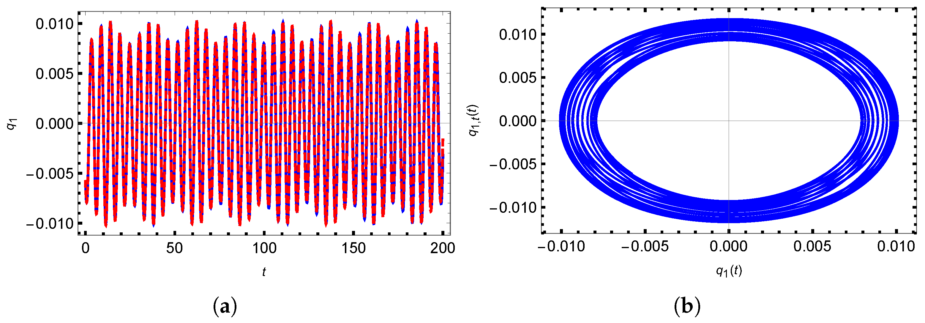
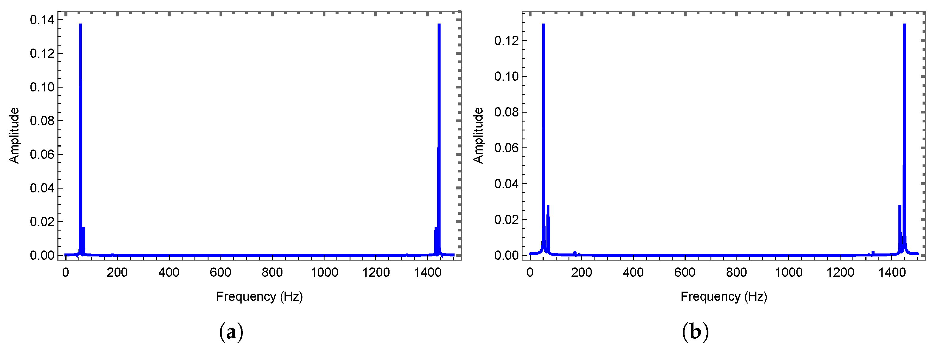
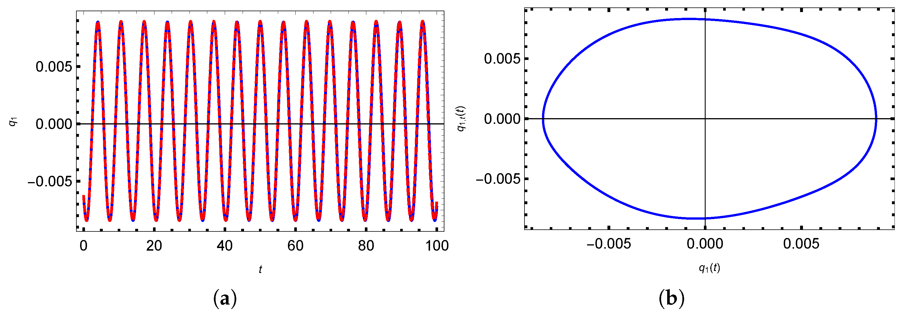
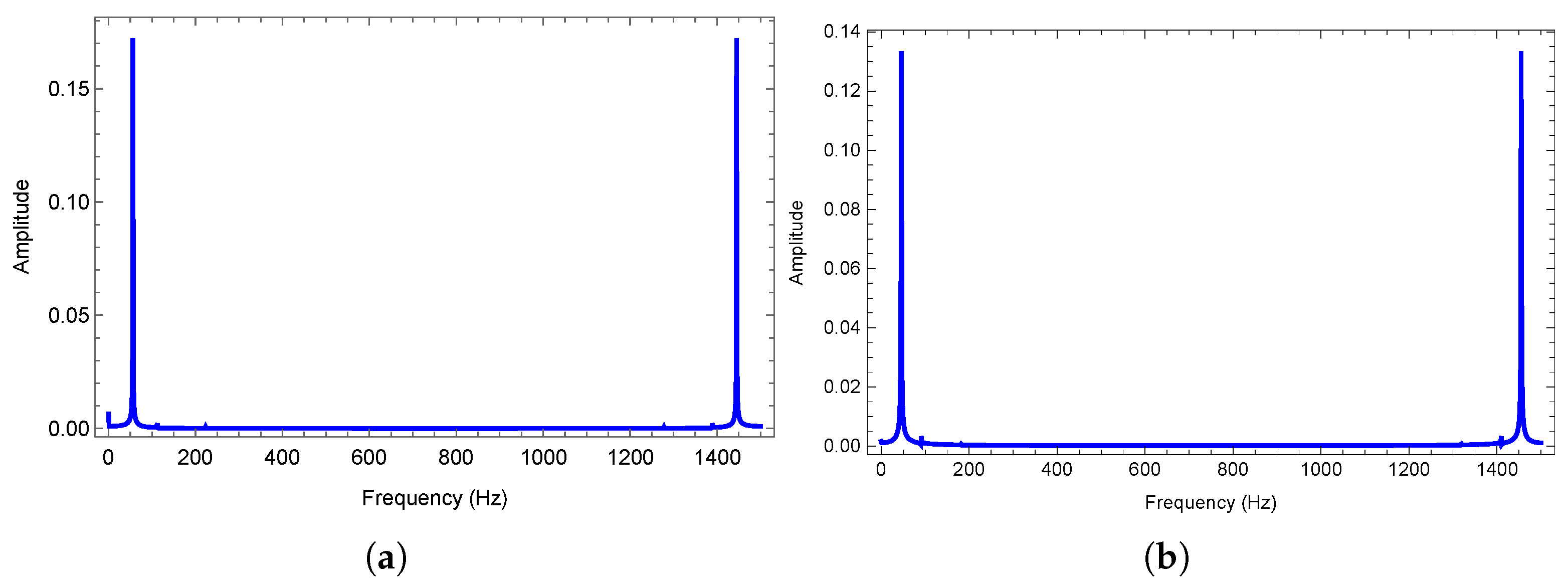
3.1. Quasi-Periodic Vibration

In this subsection, the quasi-periodic vibration is first investigated based on the double multiple-scales method. Time traces and phase-plane portraits of $q_1\left(t\right)$ for different given parameters are shown in Figure 2 and Figure 3. According to Figure 2a and Figure 3a, one can find that the results obtained from the double multiple-scales method are in excellent agreement with those of direct time integration. It means that the analytical solution obtained by the multiple-scales method is reliable. The phase-plane portraits of $q_1\left(t\right)$ for different parameters are shown in Figure 2b and Figure 3b, which indicate that the nonlinear vibration of the beam is quasi-periodic motion.

Now, the response frequency of the axially moving beam under multiple external excitations is analyzed. To this end, the fast Fourier transform is used. For Figure 2a and Figure 3a, the corresponding FFT diagrams are shown in Figure 4a and Figure 4b, respectively. In Figure 4a,b, one can find that there are two main response frequencies in the vibration of the axially moving beam, which are the combination of the natural frequencies ${\omega }_1,\mathsf{\Omega },{\mathsf{\Omega }}_2$. The two response frequencies are $({\omega }_1+{\displaystyle \frac{3\mathsf{\Omega }}{2}}-{\mathsf{\Omega }}_2)$ and $(2{\omega }_1+{\displaystyle \frac{\mathsf{\Omega }}{4}}+7{\mathsf{\Omega }}_2)$ in Figure 4a. Obviously, the response frequency is the irreducible combination of the excitation frequencies. So, the axially moving beam exhibits quasi-periodic motion as shown in Figure 2a. For Figure 4b, there is a similar conclusion. Two response frequencies $({\omega }_1+\mathsf{\Omega }-{\displaystyle \frac{61}{18}}{\mathsf{\Omega }}_2)$ and $({\omega }_1+\mathsf{\Omega }-{\displaystyle \frac{29}{9}}{\mathsf{\Omega }}_2)$ are shown for the given parameters.

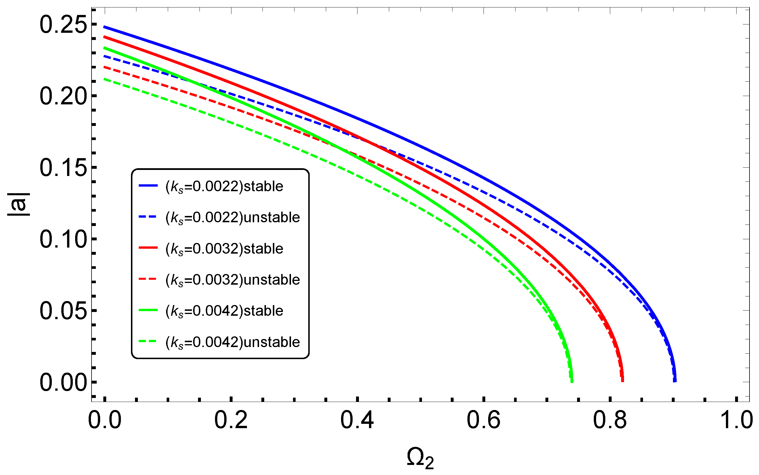
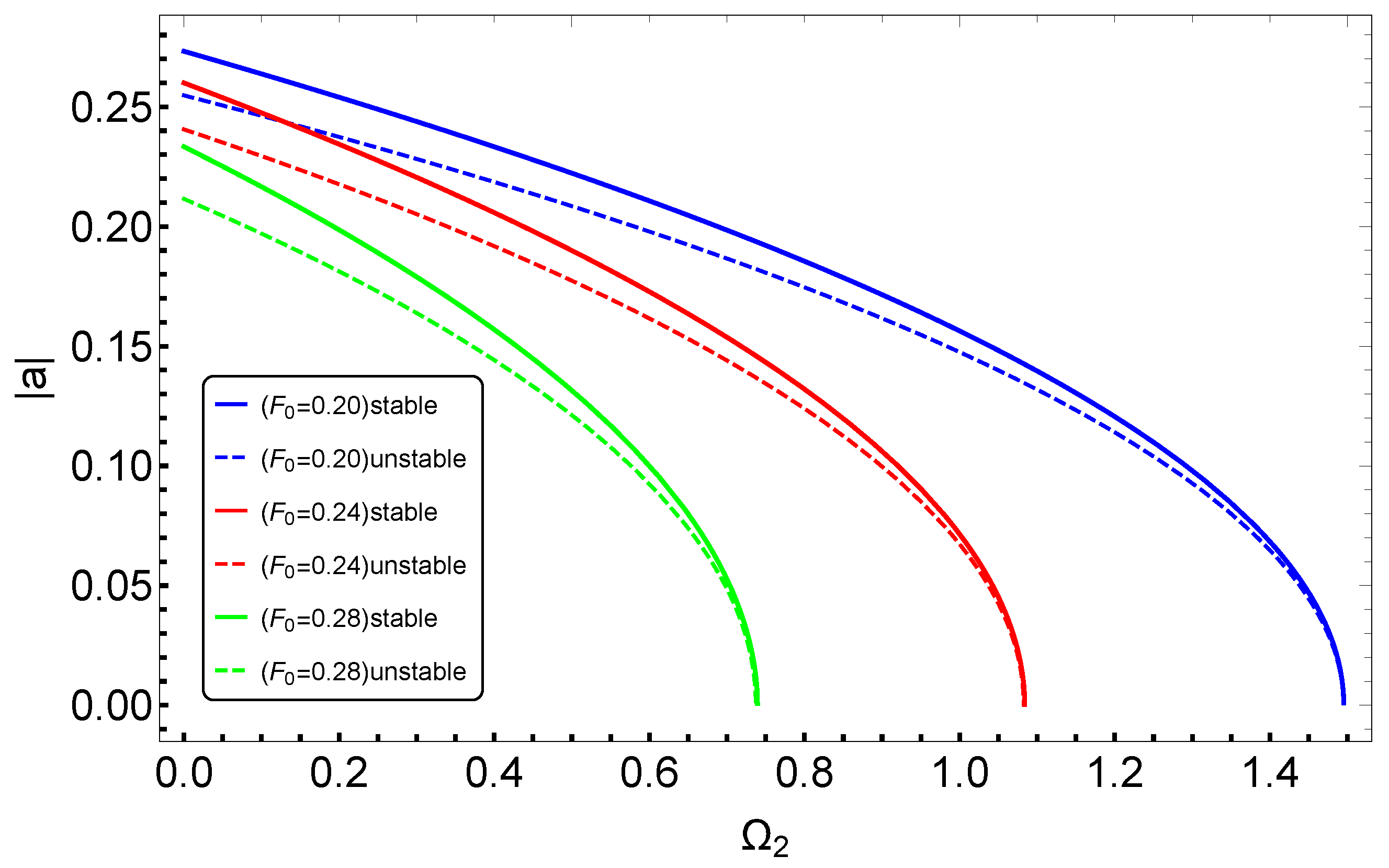
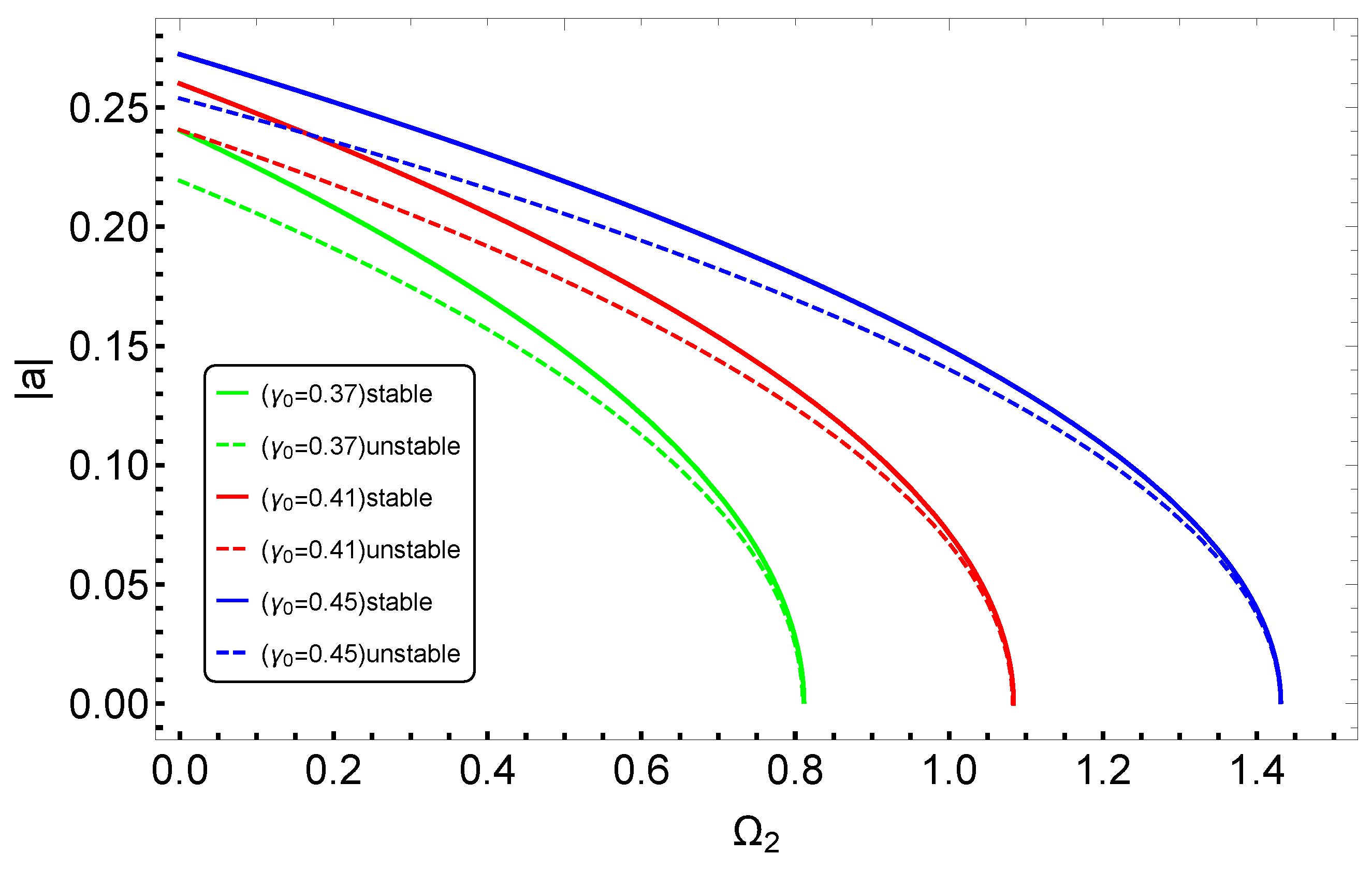
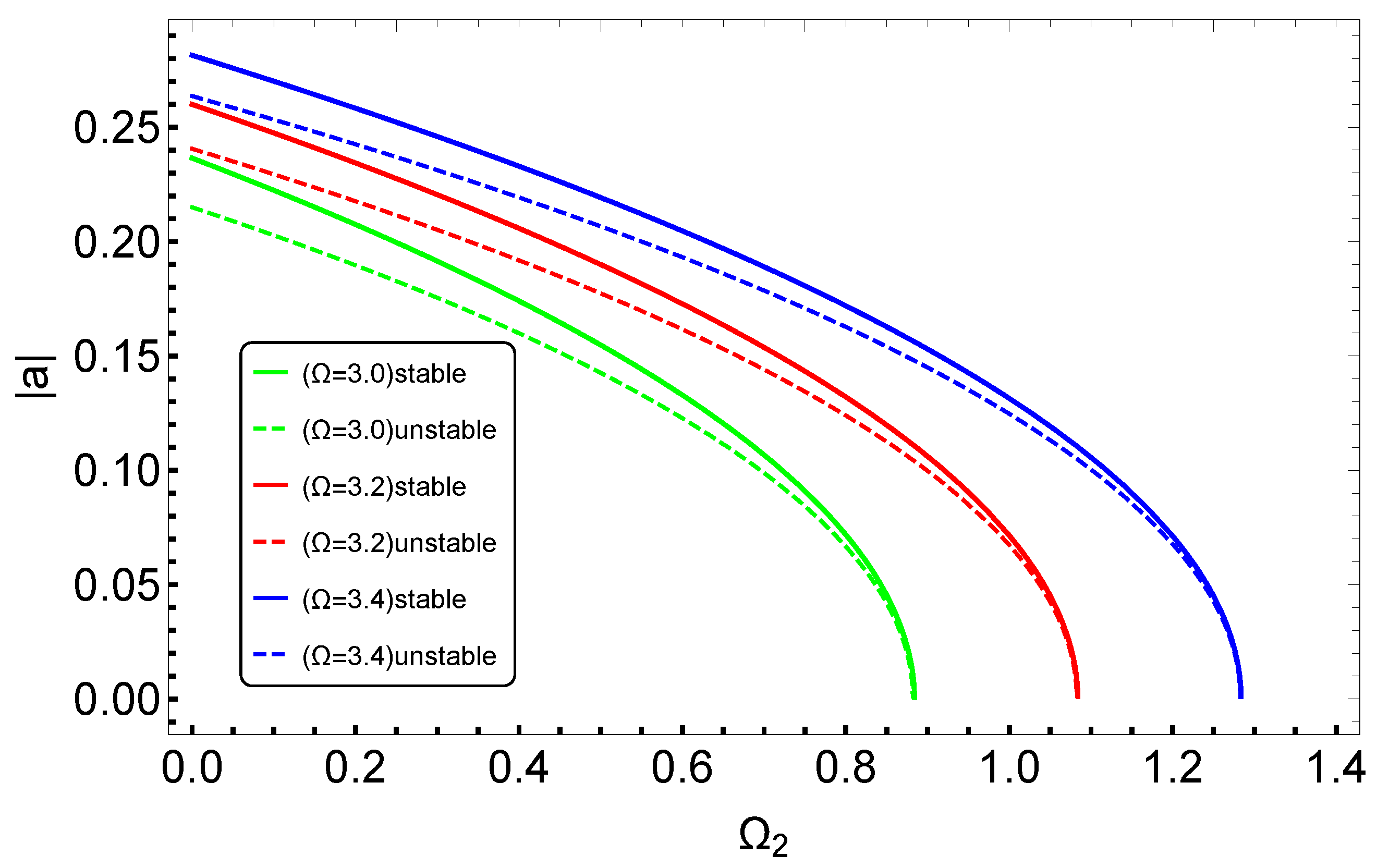
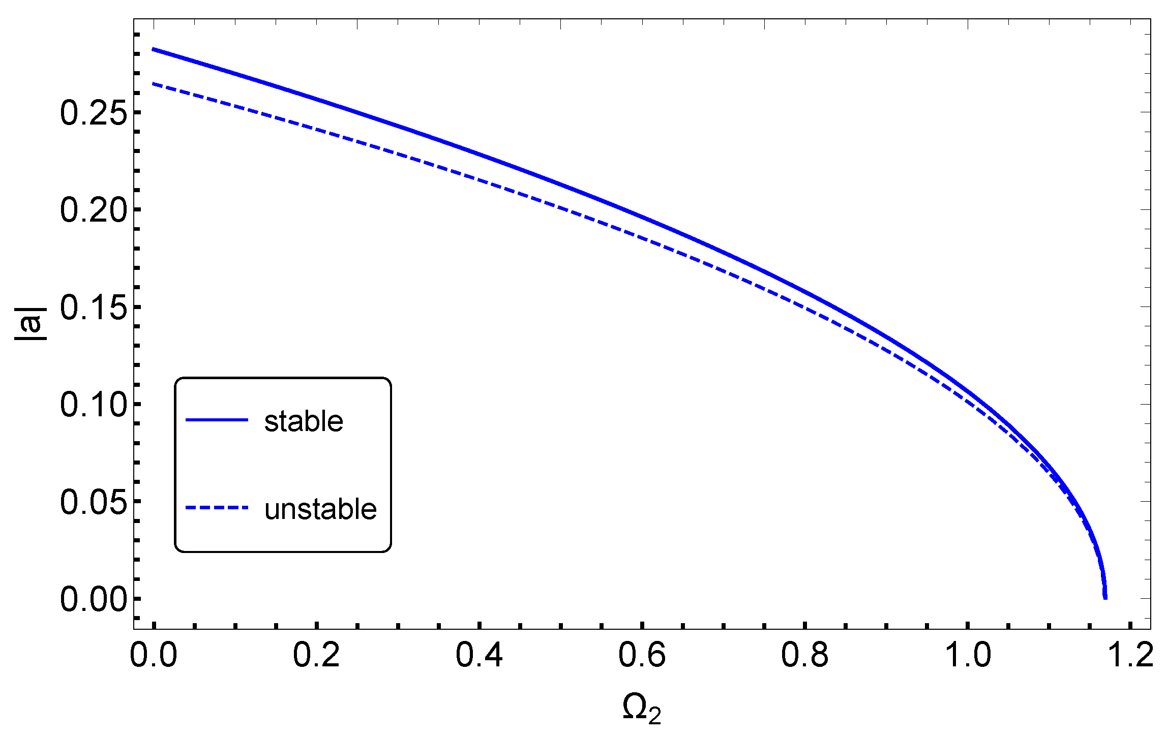
3.2. Effects of System Parameters

In this subsection, the effects of some system parameters on the frequency–amplitude response are analyzed. During the numerical experiments, some parameters are fixed at ${\gamma }_0=0.41,\mathsf{\Omega }=3.2,{\gamma }_1=0.02$ and $F_1=0.0045$. Firstly, the effect of $k_s$ on the frequency–amplitude response is investigated and the results are plotted in Figure 5. In this figure, blue, red, and green lines represent $k_s=0.0022,0.0032,0.0042$, respectively; the solid lines and the dotted lines represent the stable solutions and the unstable solutions. $k_s$ represents the thickness of the axially moving beam. It shows that the vibration amplitude of the beam decreases with the increasing geometric parameter. In other words, the vibration of a thicker axially moving beam is smaller than that of a slender axially moving beam. Furthermore, one can find that the amplitude decreases with an increase in the external excitation frequency ${\mathsf{\Omega }}_2$. Hereafter, the solid and dotted lines denote the stable and unstable responses in the next figures.

For $k_s=0.0042,{\gamma }_0=0.41,\mathsf{\Omega }=3.2,{\gamma }_1=0.02$ and $F_1=0.0045$, the effect of the external force $F_0$ on the frequency–amplitude response is shown in Figure 6. In this figure, blue, red, and green lines represent $F_0=0.20,0.24,0.28$, respectively. $F_0$ represents the initial transverse force of the axially moving beam. One can find that the vibration amplitude of the axially moving beam decreases with an increase in the $F_0$. That is, the greater the initial transverse force applied to the axially moving beam, the smaller the vibration amplitude. This figure shows that the external force plays a very important role in determining the vibration amplitude of the axially moving beam.

Now, the effect of ${\gamma }_0$ on the steady-state response is investigated. Let $k_s=0.0042,$ $F_0=0.24,\mathsf{\Omega }=3.2,{\gamma }_1=0.02$ and $F_1=0.0045$ and ${\gamma }_0=0.37,0.41,0.45$; the results are plotted in Figure 7. In this figure, blue, red, and green lines represent ${\gamma }_0=0.45,0.41,0.37$, respectively. ${\gamma }_0$ represents the initial velocity of the axially moving beam. The figure shows that the vibration amplitude of the beam increases with the growth of the ${\gamma }_0$. This indicates that the larger the initial velocity, the more easily the vibrational phenomena can be observed. Stable solutions are always larger than unstable solutions. When ${\gamma }_0=0.37$, the maximum value of ${\mathsf{\Omega }}_2$ is approximately 0.8, and when ${\gamma }_0$ is equal to 0.45, the maximum value of ${\mathsf{\Omega }}_2$ is around 1.5. Relatively speaking, parameters $F_0$ and ${\gamma }_0$ have a more significant influence on the vibration amplitude of the axially moving beam than $k_s$.

Lastly, the effect of $\mathsf{\Omega }$ of the steady-state response is analyzed. In the calculations, the system parameters are fixed at $k_s=0.0042,F_0=0.24,{\gamma }_0=0.41,{\gamma }_1=0.02$ and $F_1=0.0045$, and $\mathsf{\Omega }=3.0,3.2,3.4$. In this figure, blue, red, and green lines represent $\mathsf{\Omega }=3.4,3.2,3.0$, respectively. Figure 8 shows that the vibration amplitude of the beam increases with an increase in the parameter $\mathsf{\Omega }$. $\mathsf{\Omega }$ represents the velocity excitation frequency of the axially moving beam. This indicates that the larger the velocity excitation frequency, the greater the amplitude of vibration. It also means that the stability of the beam can be enhanced by increasing the frequency $\mathsf{\Omega }$. From this figure, which clearly shows that the same $\mathsf{\Omega }$ is taken, the values of the stable and unstable states become closer as ${\mathsf{\Omega }}_2$ increases, and are almost equal at the maximum value of ${\mathsf{\Omega }}_2$.

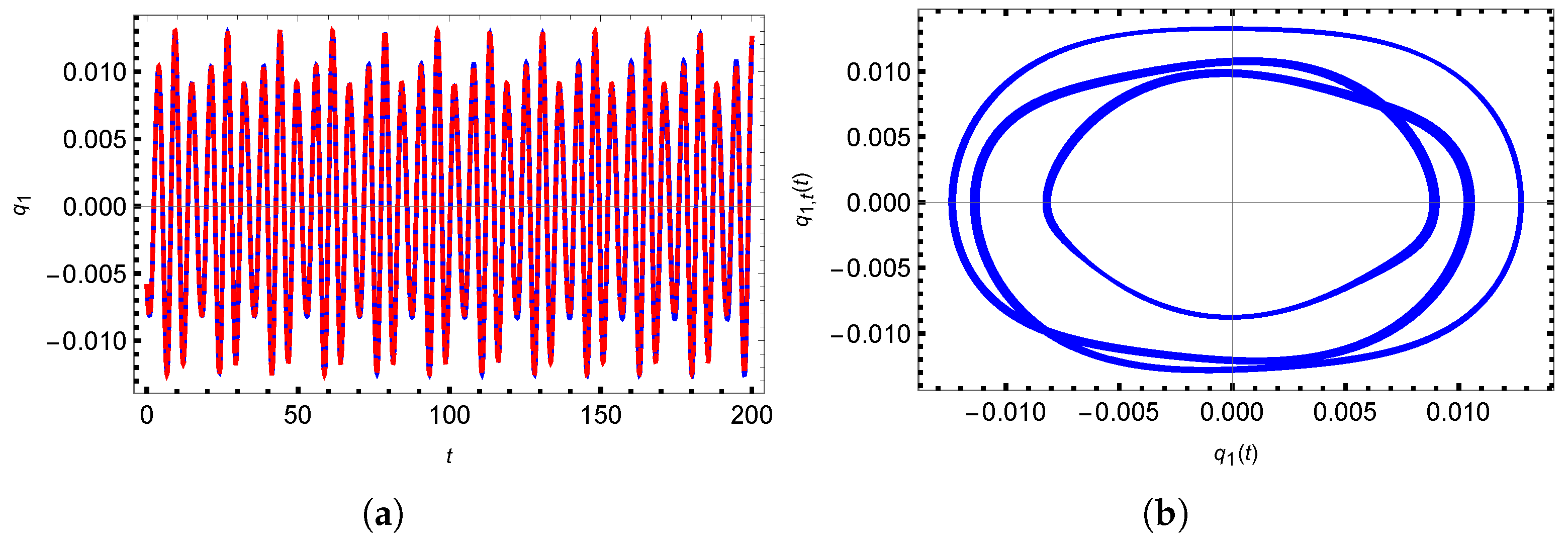
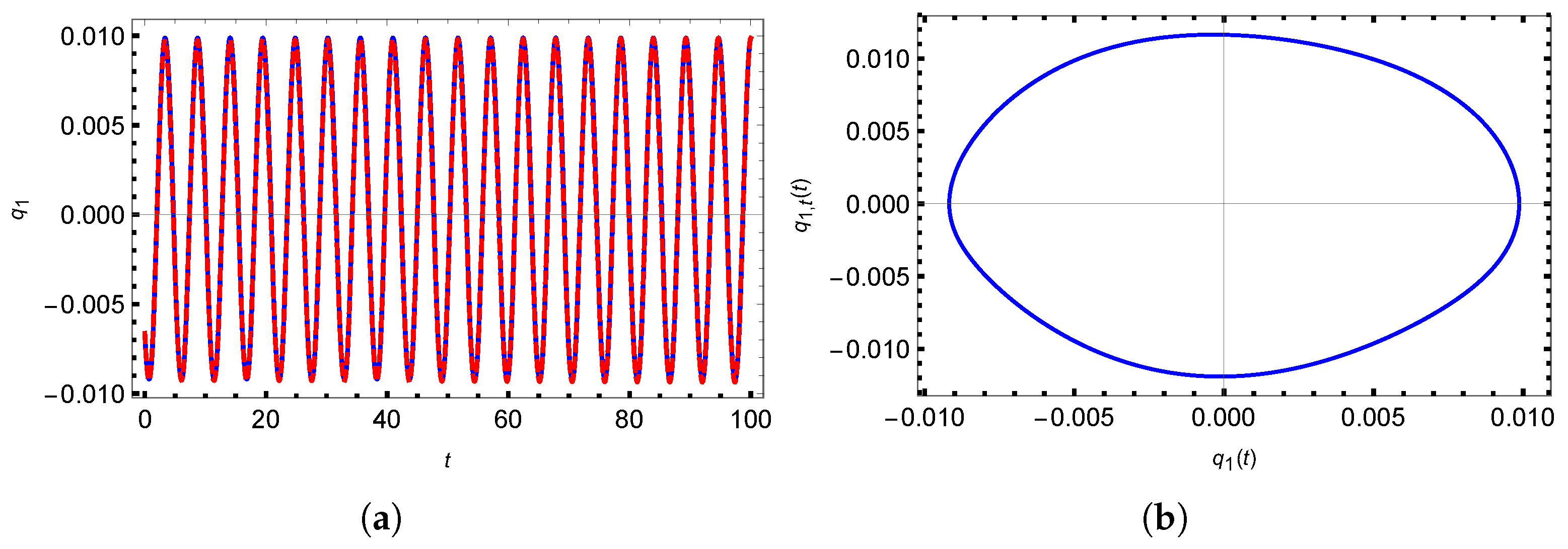
3.3. Periodic Vibration

For some given parameters, the axially moving beam will exhibit periodic motion. For example, the periodic motion can be observed for $k_s=0.0027,F_0=0.28,F_1=0.0045,$ ${\gamma }_0=0.41,{\gamma }_1=0.02,\mathsf{\Omega }=3.508,{\mathsf{\Omega }}_2=1.169$. The time history and phase-plane portraits of solution $q_1(x,t)$ for different parameters are shown in Figure 9 and Figure 10. From Figure 9a and Figure 10a, one can again see that the results obtained from the multiple-scales method are in excellent agreement with those of direct time integration. It means that the multiple-scales method not only captures the quasi-periodic motion but also the periodic motion of the axially moving beam and presents reliable analytical results.

For Figure 9, its natural frequency ${\omega }_1=1.169$, $\mathsf{\Omega }=3.508$ and then ${\mathsf{\Omega }}_2=1.169$, $\mathsf{\Omega }=3{\mathsf{\Omega }}_2\simeq 3{\omega }_1$. Similarly, for Figure 10, at this time, ${\omega }_1=0.956,\mathsf{\Omega }=2.868,{\mathsf{\Omega }}_2=0.956$. The ratio of $\mathsf{\Omega }$ to ${\mathsf{\Omega }}_2$ is approximately equal to 3.

To determine the response frequency of the periodic motion, the fast Fourier transform method is used here. In Figure 11, the main response frequencies are shown. Figure 11a,b denote the FFT diagrams of Figure 9 and Figure 10, respectively. In Figure 11a, the response frequency is ${\displaystyle \frac{121}{100}}({\omega }_1+\mathsf{\Omega }+{\mathsf{\Omega }}_2)\simeq 4.813$. In Figure 11b, the response frequency is ${\displaystyle \frac{203}{200}}({\omega }_1+\mathsf{\Omega }+{\mathsf{\Omega }}_2)\simeq 4.85$, which produce the periodic solution of Figure 10.

Now, the frequency–amplitude responses of the nonlinear vibration are analyzed for $k_s=0.0027,F_0=0.28,F_1=0.0045,{\gamma }_0=0.41,{\gamma }_1=0.02,\mathsf{\Omega }=3.508$; the curves of ${\mathsf{\Omega }}_2$ versus the amplitude of the beam are shown in Figure 12. According to Equations (42) and (43), these curves are plotted within the range ${\mathsf{\Omega }}_2=[0.5,1.2]$. It can be seen in the figure that the amplitude decreases with increasing ${\mathsf{\Omega }}_2$. Inside this range, the stable and unstable solutions can be observed. The difference between stable and unstable solutions is not large, but unstable solutions are always smaller than stable solutions.

4. Conclusions

In this work, quasi-periodic and periodic vibration responses of an axially moving beam under multiple-frequency excitation are investigated. The Galerkin method is used to discretize the differential–integral modeling equation into a second-order ordinary differential equation. A double multiple-scales method is applied to obtain the analytical solution of the ordinary differential equation. Time traces and phase-plane portraits of quasi-periodic and periodic responses are obtained from the analytical solution. Comparisons are made between the analytical solution and numerical solution obtained from the direct time integration method and good agreement is found, which shows that the double multiple-scales method can capture the vibration characteristics of an axially moving beam. Frequency–amplitude response curves of the axially moving beam are obtained analytically. The effects of system parameters on the vibration are analyzed. Some results are listed as follows: (1) The axially moving beam can exhibit quasi-periodic and periodic motion under different external excitations. When the natural frequency ${\omega }_1$, velocity frequency $\mathsf{\Omega }$, and external frequency ${\mathsf{\Omega }}_2$ are irreducible, the quasi-periodic vibration can be observed, and the response frequencies are determined. The system exhibits periodic vibration, which can be observed when the velocity frequency $\mathsf{\Omega }$ is about three times the natural frequency ${\omega }_1$. (2) Through the eigenvalue method, the stability of the nonlinear vibration has been determined. (3) Lastly, the effects of the geometric parameter $k_s$, velocity ${\gamma }_0$, velocity frequency $\mathsf{\Omega }$, and external force $F_0$ on the vibration response are obtained based on analytical solutions. The results show that the amplitude vibration of the axially moving slender beam is larger than that of the thick beam. A similar result can be obtained for external force $F_0$; the vibration amplitude increases with the mean velocity ${\gamma }_0$ and velocity frequency $\mathsf{\Omega }$.

References

1. He, L.; Li, T. Undamped non-linear vibration mechanism of bolted flange joint under transverse load. J. Asian Archit. Build. Eng. 2022, 22, 1507–1532. [Google Scholar] [CrossRef]
2. Zhu, J.; Yuan, W.B.; Li, L.Y. Cross-sectional flattening-induced nonlinear damped vibration of elastic tubes subjected to transverse loads. Chaos Solitons Fractals 2021, 151, 111273. [Google Scholar] [CrossRef]
3. Ahmadi, H.; Foroutan, K. Active vibration control of nonlinear stiffened FG cylindrical shell under periodic loads. Smart Struct. Syst. 2020, 25, 643–655. [Google Scholar]
4. Jain, V.; Kumar, R.; Patel, S.N.; Dey, T. Geometrically nonlinear dynamic analysis of a damped porous microplate resting on elastic foundations under in-plane nonuniform excitation. Mech. Based Des. Struct. Mach. 2023, 52, 4553–4598. [Google Scholar] [CrossRef]
5. Hao, J.; Li, C.; Yang, T.; Yang, J.; Zhang, Y. Dynamic analysis of moving beams featuring time-varying velocity under self-excited force moving along with the end. Meccanica 2022, 57, 2905–2927. [Google Scholar] [CrossRef]
6. Alshaqaq, M.; Hawwa, M.A. Nonlinear behavior of a vibrating axially moving small-size beam under an electrostatic force. Zamm-J. Appl. Math. Mech. Angew. Math. Mech. 2020, 100, e201900104. [Google Scholar] [CrossRef]
7. Li, Y.; Hu, X.; Peng, L.; Yuan, Y. Simulation and experimental study on transverse nonlinear vibration of axially moving yarn. Text. Res. J. 2024, 00405175231224677. [Google Scholar] [CrossRef]
8. Hu, W.; Xi, X.; Song, Z.; Zhang, C.; Deng, Z. Coupling dynamic behaviors of axially moving cracked cantilevered beam subjected to transverse harmonic load. Mech. Syst. Signal Process. 2023, 204, 110757. [Google Scholar] [CrossRef]
9. Wu, Q.; Qi, G. Homoclinic bifurcations and chaotic dynamics of non-planar waves in axially moving beam subjected to thermal load. Appl. Math. Model. 2020, 83, 674–682. [Google Scholar]
10. Cao, T.; Hu, Y. Magnetoelastic primary resonance and bifurcation of an axially moving ferromagnetic plate under harmonic magnetic force. Commun. Nonlinear Sci. Numer. Simul. 2022, 117, 106974. [Google Scholar] [CrossRef]
11. Li, M.; Jiang, W.; Li, Y.; Dai, F. Steady-state response of an axially moving circular cylindrical panel with internal resonance. Eur. J. Mech.-A Solids 2022, 92, 104464. [Google Scholar] [CrossRef]
12. Liu, M.; Yao, G. Nonlinear forced vibration and stability of an axially moving beam with a free internal hinge. Nonlinear Dyn. 2024, 112, 6877–6896. [Google Scholar] [CrossRef]
13. Cheng, Y.; Wu, Y.; Guo, B.-Z. Boundary Stability Criterion for a Nonlinear Axially Moving Beam. IEEE Trans. Autom. Control 2022, 67, 5714–5729. [Google Scholar] [CrossRef]
14. Li, M.; Liu, Y.; Wang, T.; Chu, F.; Peng, Z. Adaptive synchronous demodulation transform with application to analyzing multicomponent signals for machinery fault diagnostics. Mech. Syst. Signal Process. 2023, 191, 110208. [Google Scholar]
15. Liu, K.; Zong, S.; Li, Y.; Wang, Z.; Hu, Z.; Wang, Z. Structural response of the U-type corrugated core sandwich panel used in ship structures under the lateral quasi-static compression load. Mar. Struct. 2022, 84, 103198. [Google Scholar] [CrossRef]
16. Zhi, S.; Shen, H.; Wang, T. Gearbox localized fault detection based on meshing frequency modulation analysis. Appl. Acoust. 2024, 219, 109943. [Google Scholar] [CrossRef]
17. Zhang, Z.; Ma, X. Friction-induced nonlinear dynamics in a spline-rotor system: Numerical and experimental studies. Int. J. Mech. Sci. 2024, 278, 109427. [Google Scholar] [CrossRef]
18. Zhang, D.; Tang, Y.; Liang, R.; Song, Y.; Chen, L. Internal resonance of an axially transporting beam with a two-frequency parametric excitation. Appl. Math. Mech.-Engl. Ed. 2022, 43, 1805–1820. [Google Scholar]
19. Zhang, D.; Tang, Y.; Liang, R.; Yang, L.; Chen, L.Q. Dynamic stability of an axially transporting beam with two-frequency parametric excitation and internal resonance. Eur. J. Mech. A-Solids 2021, 85, 104084. [Google Scholar] [CrossRef]
20. Raj, S.K.; Sahoo, B.; Nayak, A.R.; Panda, L.N. Nonlinear dynamics of traveling beam with longitudinally varying axial tension and variable velocity under parametric and internal resonances. Nonlinear Dyn. 2023, 111, 3113–3147. [Google Scholar] [CrossRef]
21. Zhao, Y.; Du, J.; Liu, Y. Vibration suppression and dynamic behavior analysis of an axially loaded beam with NES and nonlinear elastic supports. J. Vib. Control 2023, 29, 844–857. [Google Scholar] [CrossRef]
22. Li, X.; Hu, Y. Principal-Internal Joint Resonance of an Axially Moving Beam with Elastic Constraints and Excited by Current-Carrying Wires. Int. J. Struct. Stab. Dyn. 2024, 24, 2450125. [Google Scholar] [CrossRef]
23. Ba, Z.; Wu, M.; Liang, J. 3D dynamic responses of a multi-layered transversely isotropic saturated half-space under concentrated forces and pore pressure. Appl. Math. Model. 2020, 80, 859–878. [Google Scholar] [CrossRef]
24. Tian, R.; Wang, M.; Zhang, Y.; Jing, X.; Zhang, X. A concave X-shaped structure supported by variable pitch springs for low-frequency vibration isolation. Mech. Syst. Signal Process. 2024, 218, 111587. [Google Scholar] [CrossRef]
25. Zhao, D.; Wang, H.; Cui, L. Frequency-chirprate synchrosqueezing-based scaling chirplet transform for wind turbine nonstationary fault feature time—Frequency representation. Mech. Syst. Signal Process. 2024, 209, 111112. [Google Scholar] [CrossRef]
26. Chen, Z.; Chen, F.; Zhou, L. Slow-fast motions induced by multi-stability and strong transient effects in an accelerating viscoelastic beam. Nonlinear Dyn. 2021, 106, 45–66. [Google Scholar] [CrossRef]
27. Kobayashi, T.K.; Fujisawa, A.; Nagashima, Y.; Moon, C.; Yamasaki, K.; Nishimura, D.; Inagaki, S.; Yamada, T.; Kasuya, N.; Kosuga, Y.; et al. Correlation-estimated conditional average method and its application on solitary oscillation in PANTA. Plasma Phys. Control. Fusion 2021, 63, 032001. [Google Scholar] [CrossRef]
28. Villanueva, J. A new averaging-extrapolation method for quasi-periodic frequency refinement. Phys. Nonlinear Phenom. 2022, 438, 133344. [Google Scholar] [CrossRef]
29. Liao, H.; Zhao, Q.; Fang, D. The continuation and stability analysis methods for quasi-periodic solutions of nonlinear systems. Nonlinear Dyn. 2020, 100, 1469–1496. [Google Scholar] [CrossRef]
30. Liu, G.; Liu, J.; Wang, L.; Lu, Z. A new semi-analytical approach for quasi-periodic vibrations of nonlinear systems. Commun. Nonlinear Sci. Numer. Simul. 2021, 103, 105999. [Google Scholar] [CrossRef]
31. Huang, J.L.; Wang, T.; Zhu, W.D. An incremental harmonic balance method with two time-scales for quasi-periodic responses of a Van der Pol-Mathieu equation. Int. J. Non-Linear Mech. 2021, 135, 103767. [Google Scholar] [CrossRef]
32. Huang, J.L.; Zhang, B.X.; Zhu, W.D. Quasi-Periodic Solutions of a Damped Nonlinear Quasi-Periodic Mathieu Equation by the Incremental Harmonic Balance Method With Two Time Scales. J. Appl. Mech. Trans. ASME 2022, 89, 091009. [Google Scholar] [CrossRef]
33. Wang, Y.; Fang, X.; Ding, H.; Chen, L.Q. Quasi-periodic vibration of an axially moving beam under conveying harmonic varying mass. Appl. Math. Model. 2023, 123, 644–658. [Google Scholar] [CrossRef]
34. Nie, X.; Tan, T.; Yan, Z.; Yan, Z.; Wang, L. Revised method of multiple scales for 1:2 internal resonance piezoelectric vibration energy harvester considering the coupled frequency. Commun. Nonlinear Sci. Numer. Simul. 2022, 118, 107018. [Google Scholar] [CrossRef]
35. Sahoo, P.K.; Chatterjee, S. Nonlinear dynamics of vortex-induced vibration of a nonlinear beam under high-frequency excitation. Int. J. Non-Linear Mech. 2021, 129, 103656. [Google Scholar] [CrossRef]
36. Qian, Y.; Zhou, H. Double Hopf bifurcation analysis of time delay coupled active control system. J. Low Freq. Noise Vib. Act. Control 2024, 14613484241236646. [Google Scholar] [CrossRef]
37. Belhaq, M.; Houssni, M. Quasi-Periodic Oscillations, Chaos and Suppression of Chaos in a Nonlinear Oscillator Driven by Parametric and External Excitations. Nonlinear Dyn. 1999, 18, 1–24. [Google Scholar] [CrossRef]
38. Bayat, A.; Jalali, A.; Ahmadi, H. Nonlinear dynamic analysis and control of FG cylindrical shell fitted with piezoelectric layers. Int. J. Struct. Stab. Dyn. 2021, 21, 2150083. [Google Scholar] [CrossRef]
39. Kirrou, I.; Mokni, L.; Belhaq, M. Quasiperiodic galloping of a wind-excited tower near secondary resonances of order 2. J. Vib. Control 2017, 23, 574–586. [Google Scholar] [CrossRef]
40. Mokni, L.; Kirrou, I.; Belhaq, M. Periodic and quasiperiodic galloping of a wind-excited tower under parametric damping. J. Vib. Control 2016, 22, 145–158. [Google Scholar] [CrossRef]
41. Guennoun, K.; Houssni, M.; Belhaq, M. Quasi-Periodic Solutions and Stability for a Weakly Damped Nonlinear Quasi-Periodic Mathieu Equation. Nonlinear Dyn. 2002, 27, 211–236. [Google Scholar] [CrossRef]
42. Zarastvand, M.R.; Ghassabi, M.; Talebitooti, R. A Review Approach for Sound Propagation Prediction of Plate Constructions. Arch. Comput. Methods Eng. 2021, 28, 2817–2843. [Google Scholar] [CrossRef]
43. Pham, P.T.; Hong, K.S. Dynamic models of axially moving systems: A review. Nonlinear Dyn. 2020, 100, 315–349. [Google Scholar] [CrossRef]
Figure 1. Schematic of an axially moving beam with velocity v ( t ) and tension F ( t ) .
Mathematics 12 02608 g001
Figure 2. For k s = 0.0027 , F 0 = 0.28 , F 1 = 0.00045 , γ 0 = 0.41 , γ 1 = 0.02 , ω 1 = 1.169 , Ω = 2.6 ,   Ω 2 = 0.255 , (a) time traces and (b) phase-plane portraits of q 1 ( t ) . Red dotted and blue solid lines denote results obtained from direct time integration and the multiple-scales method, respectively.
Mathematics 12 02608 g002
Figure 3. For k s = 0.00299 , F 0 = 0.3867 , F 1 = 0.00052 , γ 0 = 0.5489 , γ 1 = 0.04 , ω 1 = 1.065 ,   Ω = 2.535 , Ω 2 = 0.36305 , (a) time traces and (b) phase-plane portraits of q 1 ( t ) . Red dotted and blue solid lines denote results obtained from direct time integration and the multiple-scales method, respectively.
Mathematics 12 02608 g003
Figure 4. Fast Fourier transform (FFT) diagrams of q 1 . (a): the corresponding FFT diagrams of q 1 for k s = 0.0027 , F 0 = 0.28 , F 1 = 0.00045 , γ 0 = 0.41 , γ 1 = 0.02 , ω 1 = 1.169 , Ω = 2.6 ,   Ω 2 = 0.255 ; (b): the corresponding FFT diagrams of q 1 for k s = 0.00299 ,   F 0 = 0.3867 , F 1 = 0.00052 , γ 0 = 0.5489 , γ 1 = 0.04 , ω 1 = 1.065 , Ω = 2.535 ,   Ω 2 = 0.36305 .
Mathematics 12 02608 g004
Figure 5. Effect of the k s on the frequency–amplitude response. From top to bottom, k s = 0.0022 , 0.0032 , 0.0042 .
Mathematics 12 02608 g005
Figure 6. Effect of the F 0 on the frequenc–amplitude response. From top to bottom, F 0 = 0.20 , 0.24 and 0.28 .
Mathematics 12 02608 g006
Figure 7. Effect of the γ 0 on the frequency response. From inside to outside, γ 0 = 0.37 , 0.41 , 0.45 .
Mathematics 12 02608 g007
Figure 8. Effect of the Ω on the frequency–amplitude response. Blue, red, and green lines represent Ω = 3.4 , 3.2 , 3.0 .
Mathematics 12 02608 g008
Figure 9. For k s = 0.0027 , F 0 = 0.28 , F 1 = 0.0045 , γ 0 = 0.41 , γ 1 = 0.02 , ω 1 = 1.169 , Ω = 3.508 ,   Ω 2 = 1.169 , (a) time traces and (b) phase-plane portraits of q 1 ( t ) . Red dotted and blue solid lines denote results obtained from direct time integration and the multiple-scales method, respectively.
Mathematics 12 02608 g009
Figure 10. For k s = 0.0025 , F 0 = 0.22 , F 1 = 0.00045 , γ 0 = 0.39 , γ 1 = 0.02 , ω 1 = 0.956 , Ω = 2.868 , Ω 2 = 0.956 , (a) time traces and (b) phase-plane portraits of q 1 ( t ) . Red dotted and blue solid lines denote results obtained from the direct time integration and the multiple-scales method, respectively.
Mathematics 12 02608 g010
Figure 11. Fast Fourier transform (FFT) diagrams of periodic solutions. (a): the corresponding FFT diagrams of q 1 for k s = 0.0027 , F 0 = 0.28 , F 1 = 0.0045 , γ 0 = 0.41 , γ 1 = 0.02 , ω 1 = 1.169 , Ω = 3.508 ,   Ω 2 = 1.169 ; (b): the corresponding FFT diagrams of q 1 for k s = 0.0025 , F 0 = 0.22   F 1 = 0.00045 , γ 0 = 0.39 , γ 1 = 0.02 , ω 1 = 0.956 , Ω = 2.868 , Ω 2 = 0.956 .
Mathematics 12 02608 g011
Figure 12. Curves of frequency–amplitude response a. Blue solid and red dotted lines represent stable and unstable solutions.
Mathematics 12 02608 g012
Disclaimer/Publisher’s Note: The statements, opinions and data contained in all publications are solely those of the individual author(s) and contributor(s) and not of MDPI and/or the editor(s). MDPI and/or the editor(s) disclaim responsibility for any injury to people or property resulting from any ideas, methods, instructions or products referred to in the content.