Integrating Sensor Embeddings with Variant Transformer Graph Networks for Enhanced Anomaly Detection in Multi-Source Data

Abstract

With the rapid development of sensor technology, the anomaly detection of multi-source time series data becomes more and more important. Traditional anomaly detection methods deal with the temporal and spatial information in the data independently, and fail to make full use of the potential of spatio-temporal information. To address this issue, this paper proposes a novel integration method that combines sensor embeddings and temporal representation networks, effectively exploiting spatio-temporal dynamics. In addition, the graph neural network is introduced to skillfully simulate the complexity of multi-source heterogeneous data. By applying a dual loss function—consisting of a reconstruction loss and a prediction loss—we further improve the accuracy of anomaly detection. This strategy not only promotes the ability to learn normal behavior patterns from historical data, but also significantly improves the predictive ability of the model, making anomaly detection more accurate. Experimental results on four multi-source sensor datasets show that our proposed method performs better than the existing models. In addition, our approach enhances the ability to interpret anomaly detection by analyzing the sensors associated with the detected anomalies.

1. Introduction

In today’s extensively digitized landscape, multi-source time series data have become essential to standardized operations in a diverse range of industries [1]. Such data, which aggregate temporal information from diverse sources, offer profound insights into system operations [2]. With the burgeoning developments in the Internet of Things (IoT), smart manufacturing, and urban intelligence ecosystems, the effective analysis and utilization of these data streams are pivotal for enhancing efficiency, averting system failures, and optimizing decision-making processes. However, the sheer volume and complexity of these data streams pose substantial monitoring and management challenges, particularly in the realm of anomaly detection.

Anomaly detection is critical for maintaining system integrity and averting potential breakdowns [3]. This becomes significantly more complex when dealing with multi-source time series data, where each data source might exhibit unique characteristics and behavior patterns [4]. The temporal dependency and correlations between data further complicate the detection of anomalies [5]. Moreover, the diversity and dynamic nature of anomalies necessitate detection methods that are both highly adaptable and capable of responding to evolving data patterns [6]. In industrial settings, abnormal conditions are often defined by monitoring the performance indicators and operating conditions of the machinery involved [7,8,9,10].

Historically, the domain of multi-source anomaly detection in time series data has been a formidable challenge, primarily due to the multi-modal nature of the data. Conventional methods such as ARIMA [11], distance-based models [12], and distributed approaches [13] have formed the backbone of research in this field for many years. Classical methodologies like PCA [14] and deep learning approaches like DeepLSTM [15], which employs advanced LSTM networks for tasks like ECG signal anomaly detection, have shown considerable effectiveness. Similarly, MTAD-GAT [16] utilizes dual graph attention layers for capturing anomalies in multivariate time series. However, while these methods are effective in simpler scenarios, they often struggle to capture the complex non-linear relationships inherent in multi-source time series, highlighting the need for more sophisticated solutions [17,18].

The emergence of deep learning technologies has been a watershed moment for sequence modeling and anomaly detection, thanks to their robust feature extraction and non-linear fitting capabilities [19]. Early work by Hundman et al. [20] exploited LSTM networks to detect anomalies via prediction error analysis. Despite their benefits, LSTMs are often inadequate for the explicit modeling of interdependencies among variable pairs, a limitation that restricts their effectiveness in multi-dimensional settings. To address these limitations, convolutional neural networks and DAGMM models [21], which combine deep autoencoders with Gaussian mixture models, have been proposed for their proficiency in modeling complex spatial relationships in an unsupervised manner. The OmniAnomaly model [22] employs a variational autoencoder for end-to-source reconstruction, detecting anomalies based on reconstruction probability. However, traditional methods often treat the spatial and temporal aggregation processes separately, thereby limiting their efficiency.

Addressing these challenges, this paper introduces a novel approach for anomaly detection in multi-source time series utilizing graph neural networks. By constructing a graph that delineates the interrelationships among various data sources over time, our model exploits graph neural networks to discern complex spatial and temporal patterns. We introduce a modified positional encoding module to enhance temporal dependency capturing, coupled with a vector embedding technique that accommodates sensor data heterogeneity. Furthermore, the integration of attention mechanisms allows our model to prioritize relevant information selectively, enhancing its robustness and effectiveness in anomaly detection. To tackle the complexities of data fusion, we propose a dual loss function that merges reconstruction and prediction losses. This comprehensive approach not only improves anomaly detection but also enriches our understanding of complex patterns across heterogeneous sensor data. The primary contributions of our research are as follows:

Advanced Positional Encoding: We introduce a modified positional encoding module specifically designed to bolster temporal dependency capturing, crucial for accurate anomaly detection in sequential data.

Vector Embedding for Heterogeneity: Our model includes a vector embedding technique that effectively accommodates the heterogeneity of sensor data, enabling a more nuanced understanding and processing of disparate data types.

Dual Loss Function: To manage the complexities of data fusion, we have developed a dual loss function that synergistically merges reconstruction and prediction losses, thereby refining both the accuracy and reliability of anomaly detection.

Comprehensive Review and Comparison: In response to the existing literature gaps, this paper reviews an expanded range of studies pertinent to multi-domain knowledge fusion and anomaly detection, comparing the proposed methods against contemporary models to underline our approach’s novelty and effectiveness.

This study is structured as follows: Section 2 delineates the anomaly definition and data preprocessing procedures for multi-source time series. Section 3 elaborates on the detailed implementation of our proposed model. Section 4 expounds the extensive experimental outcomes and model interpretability. Section 5 concludes the paper.

2. Preliminary

In this study, the training dataset comprises multivariate time series data collected from N distinct sensors, captured over a series of time instants. This dataset, represented as $s_{\mathrm{train}}=\left[s_{\mathrm{train}}^{(1)},\cdots ,s_{\mathrm{train}}^{\left(T_{\mathrm{train}}\right)}\right]$, forms the foundational basis for our model training. At each discrete time instant t, the sensor readings are aggregated into an N-dimensional vector $s_{\mathrm{train} }^{(t)}\in {ℝ}^N$, incorporating data from all N sensors. In alignment with traditional unsupervised anomaly detection paradigms, it is assumed that the training data exclusively represent normal operational states.

The primary objective of this research is to detect anomalies within a test dataset, which is similarly derived from the same N sensors but spans a separate series of time instants. This test dataset is denoted as $s_{\mathrm{test}}=\left[s_{\mathrm{test}}^{(1)},\cdots ,s_{\mathrm{test}}^{\left(T_{\mathrm{test}}\right)}\right]$. The output generated using our algorithm is a sequence of binary labels, $\mathrm{a}(t)\in \{0,1\}$, wherein each label corresponds to a test time instant, indicating the presence 1 or absence 0 of an anomaly. Thus, all training data labels are set to 0. To augment the robustness and accuracy of our model, preprocessing strategies such as data normalization and conversion into time series windows are employed for both training and testing phases. Data normalization is performed using the following formula:

$$s_t\leftarrow {\displaystyle \frac{s_t-\min (s)}{\max (s)-\min (s)+{ϵ}^{\prime }}}$$

(1)

where min(s) and max(s) denote the element-wise minimum and maximum values from the training dataset, respectively. And ${ϵ}^{\prime }$ is a small constant vector set to ${10}^{-6}$ to prevent division by zero. This vital step, based on prior knowledge of data ranges, ensures that the dataset is normalized to the target range of from 0 to 1.

To enhance the training efficiency, the datasets are downsampled such that the sensor readings are consolidated into ten-second intervals, with median values across these intervals serving as representative metrics. If an anomaly is detected within these ten data points, a label value of 1 is assigned; otherwise, the label is set to 0. Formally, at any given time, t, the model’s input, denoted as $x^{(t)}\in {ℝ}^{N\times w}$ (where N denotes the number of sensors involved), is constructed using a sliding window of width w across the time series data, applied equally during both the training and testing phases. Consequently, the model’s input can be mathematically represented as follows:

$$x^{(t)}:=\left[s^{(t-w)},s^{(t-w+1)},\dots ,s^{(t-1)}\right]$$

(2)

3. Methodology

3.1. Temporal Encoding with Multi-Layer Variant Transformer

Transformer [23] has emerged as a robust architecture in the field of deep learning, widely utilized across a diverse range of tasks in natural language processing and computer vision. In this work, we introduce a distinctive adaptation of the transformer architecture, meticulously designed for anomaly detection in multivariate time series data. We have specifically refined the position encoding function to embrace the temporal dynamics inherent in multi-source time series. This recalibration involves transposing our original position-encoding framework to align more precisely with the temporal attributes of the data. Such a strategic modification enables the neural network to more effectively discern and leverage the underlying relational dynamics within time series, thereby enhancing the model’s predictive accuracy and its comprehension of temporal mechanisms.

This model incorporates a multi-head attention mechanism, enabling it to process and integrate information across varied representational subspaces and different positions within the sequence simultaneously. The architectural operations are delineated as follows:

$$I_1= \mathrm{LayerNorm} (I+\mathrm{MultiHeadAtt} (I,I,I))$$

(3)

$$I_2= \mathrm{LayerNorm} \left(I_1+\mathrm{FeedForward} \left(I_1\right)\right)$$

(4)

In the depicted algorithmic structure, $\mathrm{MultiHeadAtt} (I,I,I)$ denotes the implementation of a multi-head self-attention mechanism applied on the input matrix I, and the symbol ‘+’ represents the matrix addition. If the output does not align with the final layer, it is recursively integrated back into the architecture, thereby facilitating progression through L recursive layers. The overall algorithm architecture diagram is shown in Figure 1.

3.2. Spatial Embedding for Spatial Embedding

In a variety of sensor-based settings, it has been noted that sensors can display highly diverse characteristics and interact in complex ways. To address these challenges, our approach introduces a unique embedding vector for each sensor, denoted as $v_i\in {ℝ}^d$ for sensor $i\in \{1,2,\cdots ,N\}$, to encapsulate its distinct attributes. Initially assigned random values, these embeddings are refined during the training phase in conjunction with other model components. The similarity between these embeddings indicates a correspondence in behaviors; thus, sensors with similar embedding values are likely to be closely associated with each other. Within our model’s architecture, these embeddings serve a dual role. Firstly, they aid in learning the structural relationships between different sensors, enhancing the model’s capacity to interpret inter-sensor dynamics. Secondly, the embeddings bolster the attention mechanism through enabling focused attention processes across adjacent sensors, effectively accommodating the inherent heterogeneity among different types of sensors. Ultimately, the model outputs a spatial representation of the multi-source sensors, symbolized as $v=\{v_1,v_2,...,v_N\}$.

3.3. Graph Structure Learning

A fundamental aim of our framework is to elucidate the complex interconnections among sensors, conceptualized through the implementation of a graph topology. GNN employs a Message Passing Mechanism for inter-node information exchange. Specifically, each node aggregates information from its neighboring nodes and updates its own state using an aggregation function (e.g., summation, average). This iterative process continues until the network reaches a stable state. In this study, we leverage GNNs to capture spatio-temporal relationships in sensor networks, particularly for large-scale sensor data with intricate connectivity patterns. The utilization of GNNs enables the model to learn the intricate interactions between each sensor (node) and its surrounding neighbor nodes, thereby enhancing the accuracy and efficiency of anomaly detection. To achieve this, we employ a directed graph architecture [24], where nodes represent individual sensors and the edges define the dependency relations among them. Each sensor $i$ is associated with a set of potential relations $R_i$, which enumerate the sensors upon which it may depend, encapsulating our prior domain knowledge:

$$R_i\subseteq \{1,2,\cdots ,i-1,i+1,\cdots ,N\}$$

(5)

In scenarios devoid of specific priors, the potential relations for sensor $i$ include all others within the network. To discern the dependencies of sensor $i$, we assess the similarity between its embedding vector and those of potential dependent nodes $j$ using

$$e_{ji}={\displaystyle \frac{v_i^{\top }{v}_j}{‖v_i‖\cdot ‖v_j‖}} \mathrm{for} j\in R_i$$

(6)

The designation $A_{ji}$ determines whether node $j$ is amongst the top k nodes, with similarity scores highest relative to node $i$, outlined as follows:

$$A_{ji}=1\left\{j\in \mathrm{TopK}\left(\left\{e_{ki}:k\in R_i\right\}\right)\right\}$$

(7)

The analysis commences with the computation of $e_{ji}$, which represents the normalized dot product between the embedding vectors of sensor $i$ and its potential relation $j$. We then identify the top k normalized values, where $\mathrm{TopK}$ delineates the indices within its domain. The selection parameter k, which governs the network’s sparsity, is adjustable; for this study, a predefined value of 20 has been assigned to k. The value of k can be determined based on the desired sparsity level, and after conducting grid search experiments to balance algorithm efficiency and accuracy, we opted to set the value of k to this value. Integrating sensor embedding vectors $v_i$, our model captures diverse behavior characteristics of different sensor types. The synthesis of node $i$’ s composite representation $z_i^{(t)}$ is hence formulated as follows:

$$z_i^{(t)}=\mathrm{ReLU}\left({\alpha }_{i,i}W{x}_i^{(t)}+{\displaystyle \sum _{j\in \mathcal{N}(i)}{\alpha }_{i,j}}W{x}_j^{(t)}\right)$$

(8)

Here, $x_i^{(t)}\in {ℝ}^w$ presents the intrinsic feature of node $i$, $\mathcal{N}(i)$ = $\left\{j|A_{ji}>0\right\}$ represents the neighborhood derived from adjacency matrix A, and $W\in {ℝ}^{d\times w}$ is a uniform linear transformation matrix applicable across all nodes. The ${\alpha }_{i,j}$ coefficients, crucial for the attention mechanism, are computed through

$$g_i^{(t)}=(I_2\oplus v_i)\oplus W{x}_i^{(t)}$$

(9)

$$\pi (i,j)=\mathrm{LeakyReLU}\left(a^{\top }\left(g_i^{(t)}\oplus g_j^{(t)}\right)\right)$$

(10)

$${\alpha }_{i,j}={\displaystyle \frac{\exp (\pi (i,j))}{{\displaystyle \sum _{k\in \mathcal{N}(i)\cup \left\{i\right\}}\exp }(\pi (i,k))}}$$

(11)

In these expressions, $\oplus$ signifies concatenation, $a$ denotes a vector of trainable coefficients tuned for the attention schema, and LeakReLU [25] is the employed non-linear activation function. The attention coefficients are normalized using the softmax function depicted in Equation (11). Through this structured graph learning process, we acquire representations for all N nodes, collectively denoted as $z^{(t)}=\left\{z_1^{(t)},\cdots ,z_N^{(t)}\right\}$.

3.4. Joint Optimization

The output from the attention map is channeled into a graph convolutional network, augmenting its capability to capture the complex relationships embedded within the data. This integration fosters a more refined understanding and representation of the intricate interconnections inherent to graph-structured data. Subsequently, the processed outputs from the graph convolution network are utilized as inputs for both the reconstruction and prediction modules. For clarity, we denote the input to these modules at time t as ${\mathcal{X}}_t=H^{L_{\mathrm{gcn} }}$, where L represents the number of layers in the graph convolution network. The reconstruction module is strategically designed to comprehend the data distribution spanning the entire time series, while the prediction module focuses on forecasting future data points at ensuing timestamps. Specifically, the reconstruction loss quantifies the discrepancy between the current and reconstructed windows, whereas the prediction error measures the difference between the predicted value for the next timestamp and the corresponding observed value. During the optimization process, both reconstruction and prediction tasks are concurrently addressed. The composite loss function, which is designed to accommodate both objectives, is represented as follows:

$$\mathcal{L}={\gamma }_1{\mathcal{L}}_{\mathrm{rec} }+\left(1-{\gamma }_1\right)\times {\mathcal{L}}_{\mathrm{pred} }$$

(12)

In this formulation, ${\mathcal{L}}_{\mathrm{rec} }$ and ${\mathcal{L}}_{\mathrm{pred} }$ denote the loss functions pertinent to the reconstruction and prediction modules, respectively. The term ${\gamma }_1$ is a hyper-parameter entrusted with the role of balancing the contributions of the reconstruction and prediction efforts towards the collective learning objective.

3.5. Anomaly Score and Inference

Within the proposed model architecture, both the reconstruction and prediction modules are instrumental in delineating the system’s dynamics at each time step. The reconstruction module produces a reconstructed window, denoted as $\widehat{{\mathit{w}}_{\mathit{i}}}$, for each time series, while the prediction module outputs forecasts, represented as ${\widehat{x}}_i$. The anomaly score mechanism in our model is intricately designed to balance the outputs from these two modules, thereby enhancing the precision in anomaly detection. The anomaly score is mathematically formulated as follows:

$$\mathrm{Score}={\displaystyle \sum _{i=1}^N\frac{{\left({\mathit{w}}_{\mathit{i}}-\widehat{{\mathit{w}}_{\mathit{i}}}\right)}^2+{\gamma }_2\times {\left(x_i-{\widehat{x}}_i\right)}^2}{1+{\gamma }_2}}$$

(13)

Here, ${\gamma }_2$ is a crucial hyper-parameter that moderates the relative influence of the reconstruction and prediction modules. This parameter is optimized using a validation set, and following a meticulous grid search process, is set at 0.5 in this study. During the inference phase, the approach to anomaly detection is straightforward yet robust: a timestamp is classified as ‘abnormal’ if its anomaly score exceeds a pre-established threshold, and as ‘normal’ otherwise. The determination of this pivotal threshold is facilitated by employing the Peaks-Over-Threshold (POT) method [26], which leverages the validation set for its optimization. This comprehensive framework, encompassing both training and inference phases, is succinctly encapsulated within Algorithm 1, which serves as an indispensable guide for the practical implementation of our model.

Algorithm 1: The algorithm of proposed model
Training Stage
Input: Processed time window sequence $x=\left[x^{(1)},x^{(2)},\cdots ,x^{(t)}\right]$.
For $i$ in epoch:
	Calculate multi-source sensor embedding vectors $v$ and time representation $I_2$;
	Calculate the node feature representation $z$ and then put it into the graph network to acquire model feature representation $H^{L_{\mathrm{gcn} }}$;
	Calculate the reconstruction loss and prediction loss;
	Minimize the joint loss function.
end for
Test Stage
Input: Test time window sequence $\tilde{x}=\left[{\tilde{x}}^{(1)},{\tilde{x}}^{(2)},\cdots ,{\tilde{x}}^{(t)}\right]$.
Return: Predicted label list of $\tilde{x}$

4. Experimental Results and Discussion

In our comparative analysis, the proposed model was benchmarked against state-of-the-art models in the realm of multi-source time series anomaly detection, including notable models such as OmniAnomaly [22], GDN [24], MAD-GAN [27], MTAD-GAT [28], CAE-M [29], and DCdetector [30]. The experiments were conducted on a system equipped with an Intel Core i5-10400F CPU, 32 GB of RAM, and an NVIDIA GeForce RTX-3060 GPU procured from Xi’an, China. The software environment was based on PyTorch 1.5.1. For model training, the Adam [31] optimizer was employed with an initial learning rate set to 0.001. The window size for the input data was fixed at 15, and the model comprised three layers of the variant transformer architecture. The evaluation involved four publicly available datasets, renowned within the research community for benchmarking anomaly detection algorithms. The characteristics of these datasets are systematically presented in

Table 1. The characteristics of the datasets.

Dataset	Train	Test	Dimensions	Anomalies (%)
MSL [20]	58,317	73,729	27	10.72
SWAT [32]	496,800	449,919	51	11.98
WADI [33]	1,048,571	172,801	123	5.99
SMD [22]	708,405	708,420	38	4.16

. To ascertain the precision of our model, this study utilizes a suite of established evaluation metrics specifically tailored for anomaly detection in complex systems. These metrics include the F1-Score, Precision, and Recall, providing a comprehensive assessment of model performance across different scenarios.

4.1. Model Performance

Table 2. Comparison with existing methods on four datasets.

Methods	MSL			SWAT
	P	R	F1	P	R	F1
OmniAnomaly	0.7485	0.7289	0.7386	0.5637	0.5351	0.5490
MTAD-GAT	0.7832	0.7236	0.7522	0.7013	0.6694	0.6850
MAD-GAN	0.6211	0.7005	0.6584	0.7082	0.4587	0.5568
GDN	0.6485	0.6779	0.6629	0.7632	0.7388	0.7508
CAE-M	0.8164	0.6915	0.7882	0.8861	0.6121	0.7240
DCdetector	0.8032	0.7491	0.7752	0.8532	0.7139	0.7773
Proposed model	0.8277	0.8518	0.8396	0.8674	0.7475	0.8030
Methods	SMD			WADI
	P	R	F1	P	R	F1
OmniAnomaly	0.8189	0.8490	0.8337	0.3022	0.5705	0.3951
MTAD-GAT	0.7898	0.7300	0.7587	0.4076	0.7095	0.5178
MAD-GAN	0.8289	0.7983	0.8133	0.3497	0.8007	0.4868
GDN	0.8274	0.7768	0.8013	0.3982	0.7176	0.5122
CAE-M	0.7921	0.8014	0.7967	0.4746	0.7882	0.5925
DCdetector	0.8240	0.7964	0.8100	0.4978	0.8056	0.6154
Proposed model	0.8381	0.8539	0.8459	0.5015	0.8175	0.6216

provides a detailed comparative analysis between our proposed anomaly detection model and existing state-of-the-art methodologies for multi-source time series data anomaly detection across four distinct datasets. This assessment emphasizes metrics such as accuracy, recall rate, and F1-score. Notably, our model consistently surpasses the performance of all other models across the datasets in terms of F1-score. This superior performance is attributed to the model’s robust capability to extract spatio-temporal information and its adeptness at updating model parameters effectively using a dual loss function architecture. Furthermore, while all models exhibit a general decline in performance when tested on the WADI dataset, likely due to its diverse data modalities and extended duration, our model consistently demonstrates superior performance metrics. Our analysis further reveals that, despite the model’s lower accuracy compared to the figures reported in [24], this discrepancy can be attributed to the downsampling of our dataset as shown in Table 2, which inherently presents more challenges and diverges from the data configurations in the original study. However, our model significantly outperforms the GDN algorithm from [24] in terms of recall rate, thereby enhancing its value for industrial applications. Importantly, this paper presents unadjusted algorithm results unlike those in [24], which are adjusted for accuracy using the best strategy recommended by the original authors.

In the realm of industrial anomaly detection, particularly within extensive and complex data systems, the recall rate is more crucial than precision due to the disproportionately high costs associated with unaddressed anomalies compared to false positives. Our model’s recall rate excels across all datasets, notably achieving monumental improvement in datasets pertaining to water treatment equipment. Despite a slight underperformance in accuracy on the SWAT dataset relative to the CAE-M model—potentially due to the latter’s superior temporal feature extraction capabilities—our model’s recall rate sees at least a 13% improvement over CAE-M, underscoring our approach’s potential. This enhanced capability is largely owed to the integration of variant transformers and time embeddings in our model, which effectively manage simultaneous attunements to myriad data modalities, thus rendering it highly effective for multi-source scenarios. The running times of each algorithm are depicted in

Table 3. Comparison with existing methods on computation time (measured in seconds).

	MSL	SWAT
OmniAnomaly	46.2	77.3
MTAD-GAT	43.7	73.9
MAD-GAN	45.9	75.1
GDN	43.4	74.2
CAE-M	42.2	76.4
DCdetector	41.5	72.8
Proposed model	40.8	72.3

. Taking the MSL and SWAT datasets as examples, it is evident that our algorithm consistently demonstrates superior efficiency.

4.2. Interpretability of Model

To effectively illustrate the correlation dynamics encapsulated in our model, we visualized the node representation within the graph network. We selected the MSL dataset as a case study to this end. Given the considerable number of nodes within the model, the graph structure is articulated through its adjacency matrix, as depicted in Figure 2. This diagram distinctly highlights the sparsity of edges as dictated by the attention mechanism embedded in the graph structure. It is noteworthy that nodes with heightened weights are characterized by discontinuities and are distributed in an approximately periodic pattern, suggesting the capture of cyclic characteristics by the attention mechanism.

Further scrutiny of the anomaly scores reveals that the sensor recording the highest anomaly score often correlates with another sensor registering the second-highest score, a relationship detailed in Figure 3. This indicates that our model is adept not only at identifying anomalies by the degree of outlier deviation, but also at discerning abnormal behavioral patterns among interconnected sensors. A particular analysis segment from the MSL dataset identified sensor M-6 as exhibiting the most significant deviation in anomaly scores, marked by a five-pointed star in the visualizations. Notably, sensors M-5 and F-5, displaying the largest edge values, exhibited a robust correlation with M-6. For instance, sensors M-5 and M-6, being similar in type and function on the Mars exploration vehicle, likely influence each other’s readings, lending a degree of predictability that aligns with expert understanding. Conversely, the relationship between M-6 and F-5, which are heterogeneous sensor types on the Mars Rover and do not share explicit common attributes, provides an AI-informed perspective that enhances our understanding of the Mars Rover’s system dynamics. Inspired by these observations, we propose to develop an anomaly detection algorithm that integrates both threshold levels and abnormal behavioral patterns. This fusion aims to facilitate the earlier and more rapid detection of anomalies, potentially leading to significant advancements in predictive maintenance strategies.

4.3. Ablation Experiment

To precisely determine the essential components of our methodology, we conducted an incremental ablation study using the MSL dataset. This process involved systematically removing elements to examine their effect on the efficacy of our model. Initially, the dynamically learned graph was replaced with static, predetermined complete graph, in which every node was linked to every other node. Following this, we assessed the vital contributions of time encoding and spatial embeddings by implementing an attention mechanism devoid of these structures. The outcomes from these modifications are documented in

Table 4. Proposed model and its variants.

Method	Prec	Rec	F1
Proposed model	0.8277	0.8518	0.8396
w/o topk	0.8021	0.8256	0.8137
w/o time encoding	0.8115	0.8409	0.8259
w/o spatial embedding	0.7765	0.7994	0.7878

, presenting several critical insights. The replacement of the adaptive graph structure with a static complete graph led to a noticeable reduction in performance. This impairment underscores the value of the graph structure learner in enhancing model efficacy. Further, configurations that omitted time encoding and spatial embeddings from the attention mechanism demonstrated markedly inferior results, particularly in the absence of spatial embeddings. These findings indicate that including embedding features significantly enriches the computation of weight coefficients within the graph network. Collectively, these results reaffirm that the integration of learned graph structures, sensor embeddings, and time encoding are pivotal to the accuracy of our model. This comprehensive utilization of sophisticated components elucidates the superior performance of our approach over baseline methods.

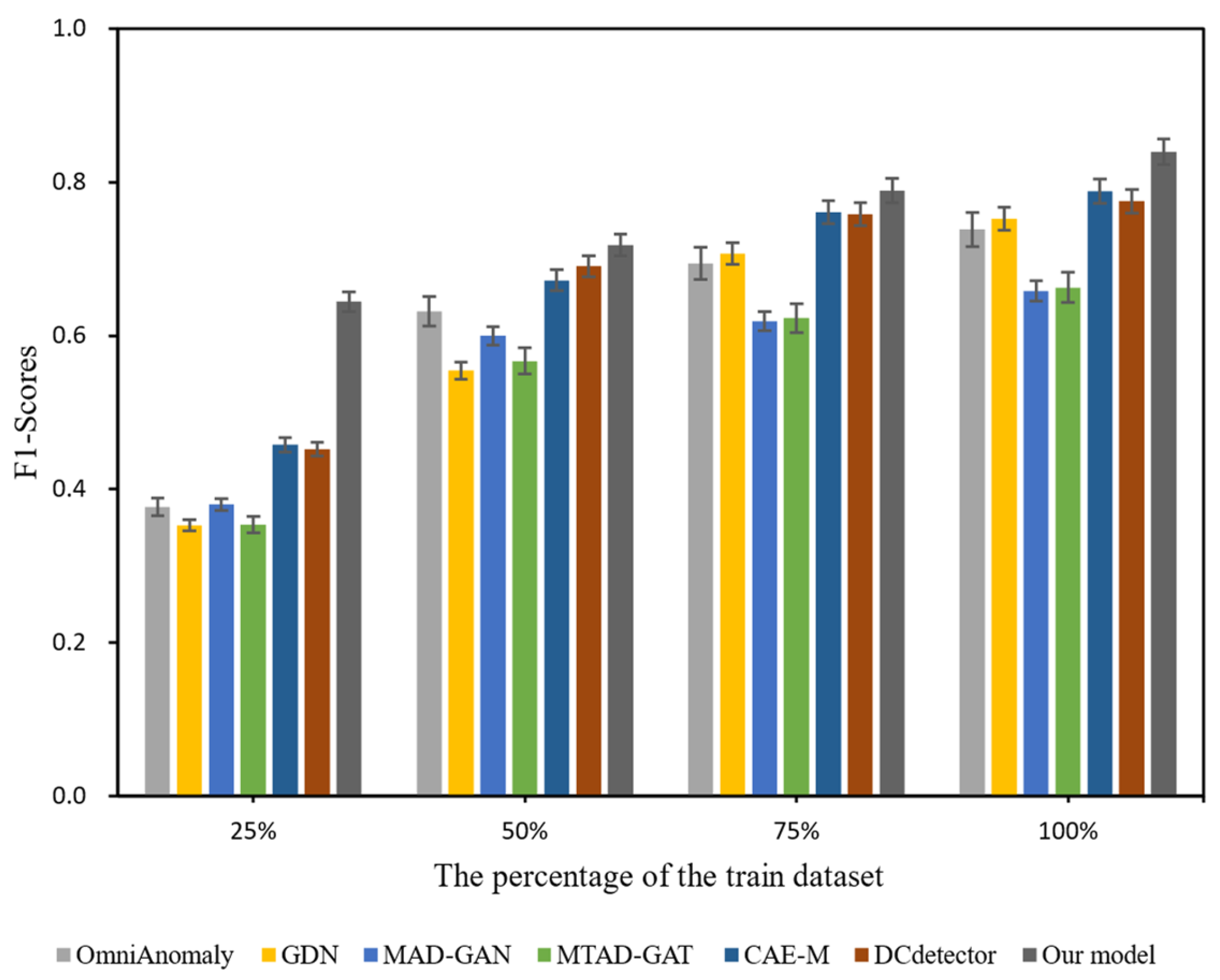
4.4. Sensitivity Analysis

We selected the MSL dataset to illustrate the stability and robustness of our model with respect to varying sizes of training data. To assess this, we conducted the experiment five times, with the training set size of randomly selected samples ranging from 25% to 100%. The results, presented in Figure 4, elucidate several important insights.

Firstly, an observable trend is that the performance of all tested methodologies decreases as the size of the training dataset diminishes. Secondly, the approach introduced in this study consistently demonstrated a superior and robust performance across all data scenarios, even when faced with limited sample sizes. This underscores the resilience of our model in scenarios characterized by data scarcity. Figure 5 sheds light on the performance of various models and their adaptations with differing analysis window sizes, which plays a pivotal role in both anomaly detection capability and training duration. It is discerned that smaller window sizes expedite the anomaly detection process due to the decreased inference time necessitated by the reduced input dimension. However, very small windows fail to capture sufficient local contextual information, while excessively large windows risk obscuring transient anomalies within an expansive array of data points. A window size of 15 strikes an optimal balance, offering an effective compromise between F1 score maximization and minimized training time. It was thus selected for use in our experiments.

5. Conclusions

Through comprehensive experiments and analysis, this study effectively demonstrates the high efficiency of the model in detecting anomalies in various sensor data sources. The findings prove that the proposed model can accurately capture the complex spatio-temporal correlations in heterogeneous sensor data, and leverage the interdependence of these data to achieve powerful event recognition capabilities beyond traditional methods. The integrated spatio-temporal framework shows significant advantages over traditional methods in improving the detection accuracy, and shows excellent performance in processing time series data and spatial relations. In addition, the superiority of the model and the interpretability of the results are verified using standard datasets. In order to further evaluate the performance, the evaluation metrics such as the precision, recall, and F1 score are introduced to deeply explore the performance of the model on different types of sensor data, and compared with several traditional and advanced anomaly detection techniques. The comparison results show that the proposed model outperforms the comparison methods in most cases, especially when dealing with high-dimensional and complex time-dependent data. Future work will extend to the early detection of subtle patterns, and this development is expected to improve the efficiency and operational safety of predictive maintenance. By introducing more real-time monitoring data and applying advanced machine learning algorithms, it is expected to further improve the prediction accuracy and scope of application of the model. Through the specific experimental data and its analysis, this study not only reveals an efficient anomaly detection method, but also provides a new perspective and technical support for sensor data processing.

References

1. Ren, H.; Xu, B.; Wang, Y.; Yi, C.; Huang, C.; Kou, X.; Xing, T.; Yang, M.; Tong, J.; Zhang, Q. Time-Series Anomaly Detection Service at Microsoft. In Proceedings of the 25th ACM SIGKDD International Conference on Knowledge Discovery & Data Mining, Anchorage, AK, USA, 4–8 August 2019; pp. 3009–3017. [Google Scholar]
2. Lin, Y.; Wang, Y. Multivariate Time Series Imputation with Bidirectional Temporal Attention-Based Convolutional Network. In Neural Computing for Advanced Applications; Zhang, H., Chen, Y., Chu, X., Zhang, Z., Hao, T., Wu, Z., Yang, Y., Eds.; Communications in Computer and Information Science; Springer Nature: Singapore, 2022; Volume 1638, pp. 494–508. ISBN 978-981-19613-4-2. [Google Scholar]
3. Schmidl, S.; Wenig, P.; Papenbrock, T. Anomaly Detection in Time Series: A Comprehensive Evaluation. Proc. VLDB Endow. 2022, 15, 1779–1797. [Google Scholar] [CrossRef]
4. Wang, P.; Li, M.; Zhi, X.; Liu, X.; He, Z.; Di, Z.; Zhu, X.; Zhu, Y.; Cui, W.; Deng, W.; et al. Deep Smooth Random Sampling and Association Attention for Air Quality Anomaly Detection. Mathematics 2024, 12, 2048. [Google Scholar] [CrossRef]
5. Králik, Ľ.; Kontšek, M.; Škvarek, O.; Klimo, M. GAN-Based Anomaly Detection Tailored for Classifiers. Mathematics 2024, 12, 1439. [Google Scholar] [CrossRef]
6. Ma, M.; Zhang, Z.; Zhai, Z.; Zhong, Z. Sparsity-Constrained Vector Autoregressive Moving Average Models for Anomaly Detection of Complex Systems with Multisensory Signals. Mathematics 2024, 12, 1304. [Google Scholar] [CrossRef]
7. Gao, J.; Song, X.; Wen, Q.; Wang, P.; Sun, L.; Xu, H. RobustTAD: Robust Time Series Anomaly Detection via Decomposition and Convolutional Neural Networks. arXiv 2020, arXiv:2002.09545. [Google Scholar]
8. Ge, D.; Dong, Z.; Cheng, Y.; Wu, Y. An Enhanced Spatio-Temporal Constraints Network for Anomaly Detection in Multivariate Time Series. Knowl.-Based Syst. 2024, 283, 111169. [Google Scholar] [CrossRef]
9. Kim, D.; Park, S.; Choo, J. When Model Meets New Normals: Test-Time Adaptation for Unsupervised Time-Series Anomaly Detection. arXiv 2024, arXiv:2312.11976. [Google Scholar] [CrossRef]
10. Mandrikova, O.; Mandrikova, B. Hybrid Model of Natural Time Series with Neural Network Component and Adaptive Nonlinear Scheme: Application for Anomaly Detection. Mathematics 2024, 12, 1079. [Google Scholar] [CrossRef]
11. Zhang, G.P. Time Series Forecasting Using a Hybrid ARIMA and Neural Network Model. Neurocomputing 2003, 50, 159–175. [Google Scholar] [CrossRef]
12. Keogh, E.; Lin, J.; Fu, A. HOT SAX: Efficiently Finding the Most Unusual Time Series Subsequence. In Proceedings of the Fifth IEEE International Conference on Data Mining (ICDM’05), Houston, TX, USA, 27–30 November 2005; pp. 226–233. [Google Scholar]
13. Ting, K.M.; Xu, B.-C.; Washio, T.; Zhou, Z.-H. Isolation Distributional Kernel A New Tool for Point & Group Anomaly Detection. IEEE Trans. Knowl. Data Eng. 2021, 35, 2697–2710. [Google Scholar] [CrossRef]
14. Shyu, M.-L.; Chen, S.-C.; Sarinnapakorn, K.; Chang, L. A Novel Anomaly Detection Scheme Based on Principal Component Classifier. In Proceedings of the IEEE Foundations and New Directions of Data Mining Workshop, Melbourne, FL, USA, 19–22 November 2003. [Google Scholar]
15. Chauhan, S.; Vig, L. Anomaly Detection in ECG Time Signals via Deep Long Short-Term Memory Networks. In Proceedings of the 2015 IEEE International Conference on Data Science and Advanced Analytics (DSAA), Paris, France, 19–21 October 2015; pp. 1–7. [Google Scholar]
16. Zhao, H.; Wang, Y.; Duan, J.; Huang, C.; Cao, D.; Tong, Y.; Xu, B.; Bai, J.; Tong, J.; Zhang, Q. Multivariate Time-Series Anomaly Detection via Graph Attention Network. In Proceedings of the 2020 IEEE International Conference on Data Mining (ICDM), Sorrento, Italy, 17–20 November 2020; pp. 841–850. [Google Scholar]
17. Ding, C.; Sun, S.; Zhao, J. MST-GAT: A Multimodal Spatial–Temporal Graph Attention Network for Time Series Anomaly Detection. Inf. Fusion 2023, 89, 527–536. [Google Scholar] [CrossRef]
18. Belay, M.A.; Blakseth, S.S.; Rasheed, A.; Salvo Rossi, P. Unsupervised Anomaly Detection for IoT-Based Multivariate Time Series: Existing Solutions, Performance Analysis and Future Directions. Sensors 2023, 23, 2844. [Google Scholar] [CrossRef] [PubMed]
19. Li, T.; Kou, G.; Peng, Y.; Yu, P.S. An Integrated Cluster Detection, Optimization, and Interpretation Approach for Financial Data. IEEE Trans. Cybern. 2022, 52, 13848–13861. [Google Scholar] [CrossRef] [PubMed]
20. Hundman, K.; Constantinou, V.; Laporte, C.; Colwell, I.; Soderstrom, T. Detecting Spacecraft Anomalies Using LSTMs and Nonparametric Dynamic Thresholding. In Proceedings of the 24th ACM SIGKDD International Conference on Knowledge Discovery & Data Mining, London, UK, 19–23 August 2018; pp. 387–395. [Google Scholar]
21. Zong, B.; Song, Q.; Min, M.R.; Cheng, W.; Lumezanu, C.; Cho, D.; Chen, H. Deep autoencoding gaussian mixture model for unsupervised anomaly detection. In Proceedings of the International Conference on Learning Representations, Vancouver, BC, Canada, 30 April–3 May 2018. [Google Scholar]
22. Su, Y.; Zhao, Y.; Niu, C.; Liu, R.; Sun, W.; Pei, D. Robust Anomaly Detection for Multivariate Time Series through Stochastic Recurrent Neural Network. In Proceedings of the 25th ACM SIGKDD International Conference on Knowledge Discovery & Data Mining, Anchorage, AK, USA, 4–8 August 2019; pp. 2828–2837. [Google Scholar]
23. Vaswani, A.; Shazeer, N.; Parmar, N.; Uszkoreit, J.; Jones, L.; Gomez, A.N.; Kaiser, Ł.; Polosukhin, I. Attention Is All You Need. In Proceedings of the 31st International Conference on Neural Information Processing Systems, Red Hook, NY, USA, 4–9 December 2017; pp. 6000–6010. [Google Scholar]
24. Deng, A.; Hooi, B. Graph Neural Network-Based Anomaly Detection in Multivariate Time Series. AAAI 2021, 35, 4027–4035. [Google Scholar] [CrossRef]
25. Xu, J.; Li, Z.; Du, B.; Zhang, M.; Liu, J. Reluplex Made More Practical: Leaky ReLU. In Proceedings of the 2020 IEEE Symposium on Computers and Communications (ISCC), Rennes, France, 7–10 July 2020; pp. 1–7. [Google Scholar]
26. Siffer, A.; Fouque, P.-A.; Termier, A.; Largouet, C. Anomaly Detection in Streams with Extreme Value Theory. In Proceedings of the 23rd ACM SIGKDD International Conference on Knowledge Discovery and Data Mining, Halifax, NS, Canada, 13 August 2017; pp. 1067–1075. [Google Scholar]
27. Li, D.; Chen, D.; Jin, B.; Shi, L.; Goh, J.; Ng, S.-K. MAD-GAN: Multivariate Anomaly Detection for Time Series Data with Generative Adversarial Networks. In Artificial Neural Networks and Machine Learning—ICANN 2019: Text and Time Series; Tetko, I.V., Kůrková, V., Karpov, P., Theis, F., Eds.; Lecture Notes in Computer Science; Springer International Publishing: Cham, Switzerland, 2019; Volume 11730, pp. 703–716. ISBN 978-3-030-30489-8. [Google Scholar]
28. Belay, M.A.; Rasheed, A.; Rossi, P.S. MTAD: Multiobjective Transformer Network for Unsupervised Multisensor Anomaly Detection. IEEE Sens. J. 2024, 24, 20254–20265. [Google Scholar] [CrossRef]
29. Zhang, Y.; Chen, Y.; Wang, J.; Pan, Z. Unsupervised Deep Anomaly Detection for Multi-Sensor Time-Series Signals. IEEE Trans. Knowl. Data Eng. 2021, 35, 2118–2132. [Google Scholar] [CrossRef]
30. Yang, Y.; Zhang, C.; Zhou, T.; Wen, Q.; Sun, L. DCdetector: Dual Attention Contrastive Representation Learning for Time Series Anomaly Detection. In Proceedings of the 29th ACM SIGKDD Conference on Knowledge Discovery and Data Mining, Long Beach, CA, USA, 6–10 August 2023; pp. 3033–3045. [Google Scholar]
31. Kingma, D.P.; Ba, J. Adam: A Method for Stochastic Optimization. arXiv 2017, arXiv:1412.6980. [Google Scholar]
32. Mathur, A.P.; Tippenhauer, N.O. SWaT: A Water Treatment Testbed for Research and Training on ICS Security. In Proceedings of the 2016 International Workshop on Cyber-physical Systems for Smart Water Networks (CySWater), Vienna, Austria, 11 April 2016; pp. 31–36. [Google Scholar]
33. Ahmed, C.M.; Palleti, V.R.; Mathur, A.P. WADI: A Water Distribution Testbed for Research in the Design of Secure Cyber Physical Systems. In Proceedings of the 3rd International Workshop on Cyber-Physical Systems for Smart Water Networks, Pittsburgh, PA, USA, 21 April 2017; pp. 25–28. [Google Scholar]
Figure 1. Architecture of the proposed model.
Mathematics 12 02612 g001
Figure 2. The adjacency matrix representation of the MSL dataset.
Mathematics 12 02612 g002
Figure 3. The topological structure of the MSL dataset.
Mathematics 12 02612 g003
Figure 4. Response to variations in training set size.
Mathematics 12 02612 g004
Figure 5. Response to variations in window size.
Mathematics 12 02612 g005