Modeling the Transmission Dynamics and Optimal Control Strategy for Huanglongbing

Abstract

Huanglongbing (HLB), also known as citrus greening disease, represents a severe and imminent threat to the global citrus industry. With no complete cure currently available, effective control strategies are crucial. This article presents a transmission model of HLB, both with and without nutrient injection, to explore methods for controlling disease spread. By calculating the basic reproduction number ($R_0$) and analyzing threshold dynamics, we demonstrate that the system remains globally stable when $R_0<1$, but persists when $R_0>1$. Sensitivity analyses reveal factors that significantly impact HLB spread on both global and local scales. We also propose a comprehensive optimal control model using the pontryagin minimum principle and validate its feasibility through numerical simulations. Results show that while removing infected trees and spraying insecticides can significantly reduce disease spread, a combination of measures, including the production of disease-free budwood and nursery trees, nutrient solution injection, removal of infected trees, and insecticide application, provides superior control and meets the desired control targets. These findings offer valuable insights for policymakers in understanding and managing HLB outbreaks.

1. Introduction

Citrus Huanglongbing (HLB) is the most destructive citrus plant disease worldwide [1]. As there are no curable chemicals and no resistant commercial citrus varieties so far, it is still the biggest threat to Chinese citrus industry [2]. Endemic in China for over a hundred years, the disease was first reported in 1913 and 1919 in Taiwan [3] and Guangdong [4], respectively. In the mainland of China, HLB has occurred in over 300 counties of 10 provinces, and has destroyed millions of hectares of Chinese citrus orchards throughout history [2].

In 2013, an outbreak of HLB occurred in Ganzhou, Jiangxi province. About 50 million diseased trees were destroyed until 2019, although integrated prevention and control measures were implemented for the 6 years in this area. HLB is caused by the bacterium Candidatus Liberibacter spp. and transmitted by Asian citrus psyllid (ACP), which acquires the virus from infected citrus trees and inoculates healthy trees with it [5,6]. HLB control strategies, such as the use of insecticides, rouging of infected trees, and production of disease-free budwood and nursery trees, have been widely implemented [7]. The use of insecticides is intended to reduce vector abundance. Rouging and removing infected hosts and producing disease-free budwood and nursery trees can reduce sources of the inoculum. As we all know, spraying an insecticide has the advantages of high efficiency and convenient use, but excessive use of pesticides leads to environmental pollution, insecticide resistance, and the death of natural predators. In addition, it is costly and difficult to replant trees and produce disease-free budwood and nursery trees, which is why producers choose not to remove diseased trees if they remain productive [8]. Recently, antibiotics have been applied by injecting them into trees in several countries or regions in attempt to control citrus HLB [9]. Injecting trees with antiviral nutrient solution is a new measure being developed to effectively curb the epidemic of HLB. It is therefore important to study the impact of integrated management on HLB disease transmission. Our goal is to build a mathematical model to study the impact of integrated management on HLB transmission and its optimal control.

Epidemiological models are suitable tools with which to understand HLB dynamics and to evaluate the effectiveness of the control measures applied. Recently, there has been progress in the modeling of the transmission process of citrus HLB disease (see, for instance, refs. [10,11,12]). The first mathematical model of HLB transmission, developed by Braga et al. [10], and most analyses performed since have focused on the effect of the control strategy used on disease dynamics. Taylor et al. [12] developed an HLB model by including temperature-dependent psyllid traits, “flushing” of trees, insecticide spraying, and economic costs to determine the most cost-effective spraying strategy. Guo et al. [13] and Liao [14] extended this work to delay differential equation models.

Recent progress in epidemiology has led to the broad application of optimal control theory in addressing infectious diseases [13,15,16,17,18,19]. For example, Odionyenma et al. [16] developed an optimal control model for gonorrhea, aimed at structured populations, and evaluated the effectiveness of control strategies, such as education, condom use, vaccination, and treatment, in reducing the spread of the disease. Zhang et al. [15] developed a model proposed in [20] to describe the dynamics and comprehensive interventions, including a detailed representation, of a psyllid population and their different stages of development (egg, larva and adult). Most of the literature on HLB models explores the major components of traditional HLB management, including rouging infected trees and spraying insecticide. Some of them use optimal control theory to design methods to limit the spread of HLB. However, few studies have applied mathematical models to investigate the effect of nutrient solution injection on the transmission of the disease.

In this paper, we use optimal control theory to study the effectiveness and cost effectiveness of all combinations of four HLB control measures, namely (1) the production of disease-free budwood and nursery trees, (2) nutrient solution injection, (3) spraying of insecticides and (4) removal of diseased trees. The model is formulated in Section 2, and a mathematical analysis of the model is presented in Section 3. The cost effectiveness and optimal control analysis are presented in Section 5, while in Section 6, we present numerical simulations of the optimal control model. Finally, a brief discussion and conclusion are presented in Section 7.

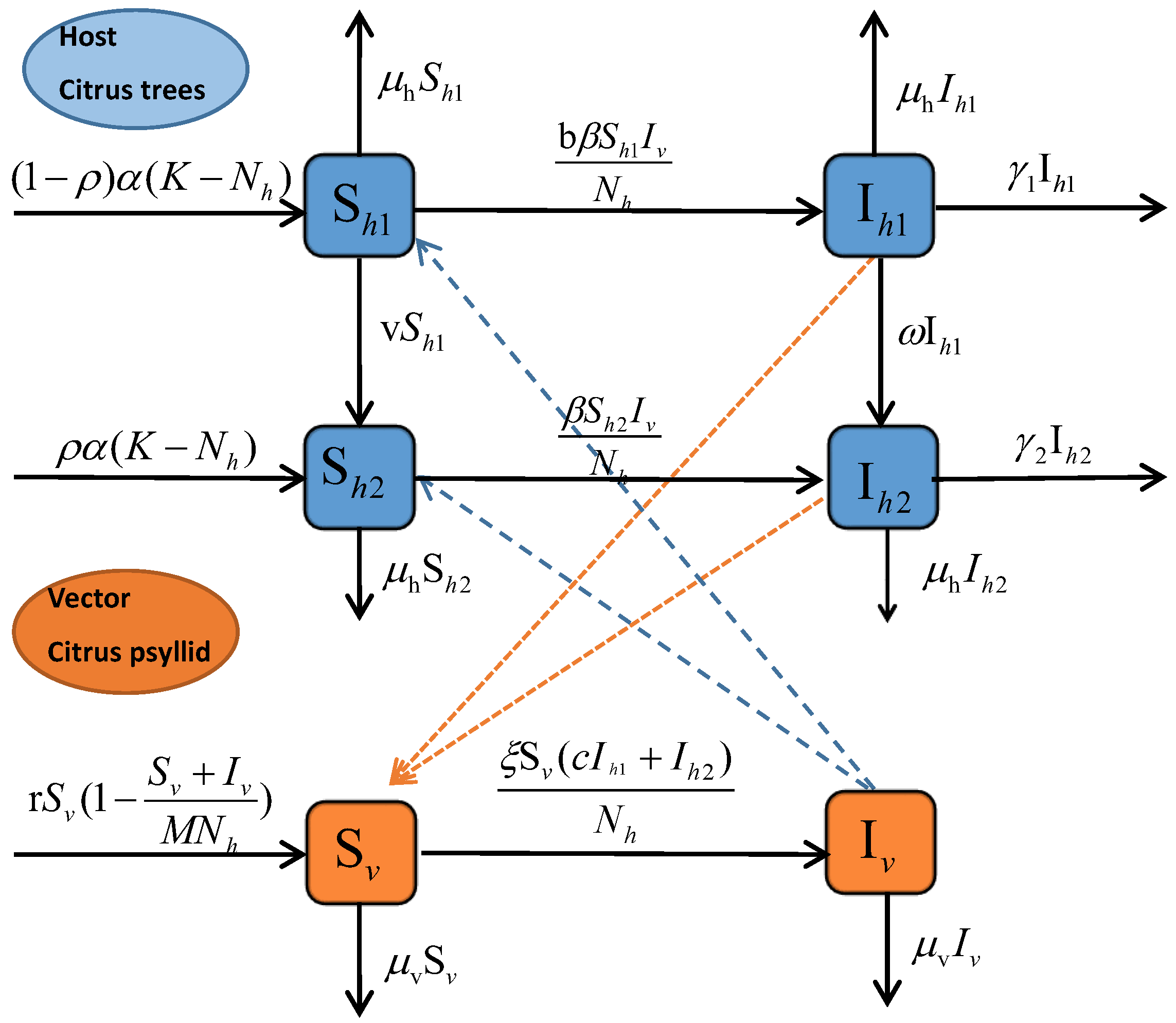
2. Model Formulation

In this section, an HLB model, where transmission occurs via a vector (citrus psyllid), is formulated and analyzed. For citrus trees, the total population under consideration is divided into four compartments: $S_{h1},S_{h2},I_{h1}$ and $I_{h2}$. $S_{h1}$ denotes susceptible citrus trees with nutrient solution treatment, and $S_{h2}$ represents susceptible citrus trees without nutrient solution treatment. $I_{h1}$ and $I_{h2}$ denote the infected citrus trees, corresponding to $S_{h1}$ and $S_{h2}$, respectively. The total number of citrus trees is $N_h\left(t\right)=S_{h1}\left(t\right)+S_{h2}\left(t\right)+I_{h1}\left(t\right)+I_{h2}\left(t\right)$. For the ACP vector population, we let $S_v$ and $I_v$ represent the susceptible and infected ACPs, respectively. $N_v\left(t\right)=S_v\left(t\right)+I_v\left(t\right)$ is the total number of ACPs. The model is schematically represented in Figure 1.

Based on Figure 1, the model for HLB transmission is formulated as follows:

$$\left\{\begin{array}{c}{\displaystyle \frac{\mathrm{d}{S}_{h1}}{\mathrm{d}t}}=(1-\rho )\alpha (K-N_h)-{\displaystyle \frac{b\beta S_{h1}{I}_v}{N_h}}-{\mu }_h{S}_{h1}-v{S}_{h1},\hfill \\ {\displaystyle \frac{\mathrm{d}{S}_{h2}}{\mathrm{d}t}}=\rho \alpha (K-N_h)-{\displaystyle \frac{\beta S_{h2}{I}_v}{N_h}}-{\mu }_h{S}_{h2}+v{S}_{h1},\hfill \\ {\displaystyle \frac{\mathrm{d}{I}_{h1}}{\mathrm{d}t}}={\displaystyle \frac{b\beta S_{h1}{I}_v}{N_h}}-({\mu }_h+{\gamma }_1)I_{h1}-\omega I_{h1},\hfill \\ {\displaystyle \frac{\mathrm{d}{I}_{h2}}{\mathrm{d}t}}={\displaystyle \frac{\beta S_{h2}{I}_v}{N_h}}-({\mu }_h+{\gamma }_2)I_{h2}+\omega I_{h1},\hfill \\ {\displaystyle \frac{\mathrm{d}{S}_v}{\mathrm{d}t}}=r{S}_v\left(1-{\displaystyle \frac{S_v+I_v}{M{N}_h}}\right)-{\displaystyle \frac{\zeta S_v(c{I}_{h1}+I_{h2})}{N_h}}-{\mu }_v{S}_v,\hfill \\ {\displaystyle \frac{\mathrm{d}{I}_v}{\mathrm{d}t}}={\displaystyle \frac{\zeta S_v(c{I}_{h1}+I_{h2})}{N_h}}-{\mu }_v{I}_v.\hfill \end{array}\right.$$

(1)

In model (1), we assume that the host recruitment to the population via replanting is proportional to the difference between the actual number of trees and maximum population size. K is the maximum number of citrus trees that can be planted in the grove, and $\alpha$ is the replanting rate. $\rho$ is the percentage of susceptible trees without nutrient solution treatment. M represents the maximum abundance of ACPs per tree. r is the oviposition rate of susceptible ACPs. $\beta$ and $\zeta$ are the infection rates due to infected ACPs on susceptible trees without nutrient solution treatment and due to infected trees with nutrient solution treatment to susceptible ACP, respectively. b denotes the decreased probability of being infected of $S_{h1}$ with respect to $S_{h2}$, and c denotes the decreased probability of infection of $I_{h1}$ with respect to $I_{h2}$. ${\mu }_h,{\mu }_v$ are the natural death rates of citrus trees and ACPs, and ${\gamma }_1$ and ${\gamma }_2$ are the disease-induced mortalities of citrus trees with and without nutrient solution treatment, respectively. We assume that the parameters v and $\omega$ are the conversion rates from $S_{h1}$ to $S_{h2}$ and from $I_{h1}$ to $I_{h2}$. All parameter values of model (1) are presented in

Table 1. Parameters for model (1).

Parameter	Baseline Value	Unit	Reference
$\rho$	0.6	${\mathrm{month}}^{-1}$	Assume
$\alpha$	0.0791	${\mathrm{month}}^{-1}$	[20]
$\beta$	0.000494	${\mathrm{month}}^{-1}$	[20]
$\zeta$	0.0197	${\mathrm{month}}^{-1}$	[20]
K	2000	-	Assume
M	3850	-	[21]
${\mu }_h$	0.0034	${\mathrm{month}}^{-1}$	[22]
${\mu }_v$	0.7	${\mathrm{month}}^{-1}$	[23]
v	0.0533	${\mathrm{month}}^{-1}$	[24]
${\delta }_2$	0.05	${\mathrm{month}}^{-1}$	Assume
$\omega$	0.0417	${\mathrm{month}}^{-1}$	[1]
r	3.714	${\mathrm{month}}^{-1}$	[25]
${\gamma }_1$	0.01	${\mathrm{month}}^{-1}$	Assume
${\gamma }_2$	0.02	${\mathrm{month}}^{-1}$	[1]
b	0.8	-	[26]
c	0.8	-	[26]
$v_1$	0.5	${\mathrm{month}}^{-1}$	Assume
$\theta$	0.5	${\mathrm{month}}^{-1}$	Assume
${\delta }_1$	0.1	${\mathrm{month}}^{-1}$	Assume

.

3. Some Useful Results

The initial conditions for system (1) take the following form:

$$S_{h1}\left(0\right)\ge 0,S_{h2}\left(0\right)\ge 0,I_{h1}\left(0\right)\ge 0,I_{h2}\left(0\right)\ge 0,S_v\left(0\right)\ge 0,I_v\left(0\right)\ge 0,N_h\left(0\right)\le K.$$

(2)

It is easy to observe that the psyllid population will die out when $r\le {\mu }_v$; hence, we assume that $r>{\mu }_v$ holds in this paper.

3.1. Positivity and Boundedness of Solutions

Biologically, it is important to show that all of the model’s state variables are non-negative at all times. In other words, all solutions of model (1) remain non-negative with initial data (2) for all $t\ge 0$.

Denote the following:

$$\begin{array}{c}{N}_h^{*}={\displaystyle \frac{\alpha K}{\alpha +{\mu }_h}},N_v^{*}={\displaystyle \frac{M{N}_h^{*}(r-{\mu }_v)}{r}},\\ \mathrm{\Gamma }=\left\{(S_{h1},S_{h2},I_{h1},I_{h2},S_v,I_v)\in {\mathcal{R}}_{+}^6|0\le N_h\le N_h^{*},0\le N_v\le N_v^{*}\right\}.\end{array}$$

Lemma 1.

Let $x\left(t\right)=(S_{h1}\left(t\right),S_{h2}\left(t\right),I_{h1}\left(t\right),I_{h2}\left(t\right),S_v\left(t\right),I_v\left(t\right))$ be the solution of system (1) with initial data (2). Then, $x\left(t\right)$ is non-negative for all $t\ge 0$. Further, the set $\mathrm{\Gamma }$ is positively invariant for system (1).

Proof. 

It is obvious that $N_h\left(t\right)\le K$. Then, from the first equation of the system (1), we have the following:

$${\left.{\displaystyle \frac{\mathrm{d}{S}_{h1}}{\mathrm{d}t}}\right|}_{S_{h1}=0,S_{h2}\ge 0,I_{h1}\ge 0,I_{h2}\ge 0,S_v\ge 0,I_v\ge 0}=(1-\rho )\alpha (K-N_h)\ge 0.$$

Therefore, $S_{h1}\left(t\right)\ge 0$, for all $t\ge 0$. Similarly, $S_{h2}\left(t\right)\ge 0,I_{h1}\left(t\right)\ge 0,I_{h2}\left(t\right)\ge 0,S_v\ge 0,I_v\left(t\right)\ge 0$ for all $t\ge 0$. Hence, it can be shown that solution $x\left(t\right)$ is non-negative for all $t\ge 0$.

Adding together the first four equations of system (1), the total number of citrus tree populations, $N_h$, satisfies the following:

$${\displaystyle \frac{\mathrm{d}{N}_h}{\mathrm{d}t}}=\alpha (K-N_h)-{\mu }_h{N}_h-{\gamma }_1{I}_{h1}-{\gamma }_2{I}_{h2}\le \alpha K-(\alpha +{\mu }_h)N_h.$$

(3)

It follows from (3) that

$$\underset{t\to \infty }{lim\; sup}{N}_h\left(t\right)\le {\displaystyle \frac{\alpha K}{\alpha +{\mu }_h}}=N_h^{*}.$$

(4)

Similarly, adding the ACP population of system (1) gives the following:

$${\displaystyle \frac{\mathrm{d}{N}_v}{\mathrm{d}t}}=r{S}_v\left(1-{\displaystyle \frac{S_v+I_v}{M{N}_h}}\right)-{\mu }_v{N}_v=r{S}_v\left(1-{\displaystyle \frac{N_v}{M{N}_h}}\right)-{\mu }_v{N}_v.$$

(5)

It follows from (4) and (5) that for a sufficiently large t,

$$\begin{array}{cc}{\displaystyle \frac{\mathrm{d}{N}_v}{\mathrm{d}t}}\hfill & =r{S}_v\left(1-{\displaystyle \frac{S_v+I_v}{M{N}_h}}\right)-{\mu }_v{N}_v\hfill \\ & \le r{N}_v\left(1-{\displaystyle \frac{N_v}{M{N}_h^{*}}}\right)-{\mu }_v{N}_v\hfill \\ & =(r-{\mu }_v)N_v-{\displaystyle \frac{r}{M{N}_h^{*}}}{N}_v^2.\hfill \end{array}$$

Thus, we have ${lim\; sup}_{t\to \infty }{N}_v\left(t\right)\le {\displaystyle \frac{M{N}_h^{*}(r-{\mu }_v)}{r}}=N_v^{*}$. Consequently, the set $\mathrm{\Gamma }$ is positively invariant for system (1). □

3.2. The Basic Reproductive Number

It is easy to observe that system (1) has a unique disease-free equilibrium (DFE) point. The DFE is obtained by turning the right-hand sides of the equations in the model (1) into zero, and is given by $P_0=\left(S_{h1}^0,S_{h2}^0,0,0,S_v^0,0\right)$, where

$$\begin{array}{c}{S}_{h1}^0={\displaystyle \frac{\alpha K(1-\rho ){\mu }_h}{\left(\alpha +{\mu }_h\right)\left({\mu }_h+v\right)}},\hfill \\ S_{h2}^0={\displaystyle \frac{\alpha K\left(\rho {\mu }_h+v\right)}{\left(\alpha +{\mu }_h\right)\left({\mu }_h+v\right)}},\hfill \\ S_v^0={\displaystyle \frac{\alpha KM\left(r-{\mu }_v\right)}{r\left(\alpha +{\mu }_h\right)}}.\hfill \end{array}$$

In order to analyze the stability of system (1), we first need to obtain the basic reproductive number, $R_0$, which is a key parameter that determines the dynamic behavior of the model. By using the next-generation operator method, which was developed by van den Driessche and Watmough [27], we can calculate the basic reproductive number, $R_0$. The rate at which new infections are introduced is determined by the matrix $\mathcal{F}$; the rates of transfer into and out of the class of infected states are represented by the matrix $\mathcal{V}$, and are given by the following:

$$\mathcal{F}=\left(\begin{array}{c}{\displaystyle \frac{b\beta I_v}{N_h}}{S}_{h1}\\ {\displaystyle \frac{\beta I_v}{N_h}}{S}_{h2}\\ {\displaystyle \frac{\zeta (c{I}_{h1}+I_{h2})}{N_h}}{S}_v\\ 0\\ 0\\ 0\end{array}\right)\mathrm{and}\mathcal{V}=\left(\begin{array}{c}({\mu }_h+{\gamma }_1)I_{h1}+\omega I_{h1}\\ ({\mu }_h+{\gamma }_2)I_{h2}-\omega I_{h1}\\ {\mu }_v{I}_v\\ {\displaystyle \frac{b\beta I_v}{N_h}}{S}_{h1}+{\mu }_h{S}_{h1}-(1-\rho )\alpha (K-N_h)+v{S}_{h1}\\ {\displaystyle \frac{\beta I_v}{N_h}}{S}_{h2}+{\mu }_h{S}_{h2}-\rho \alpha (K-N_h)-v{S}_{h1}\\ {\displaystyle \frac{\zeta (c{I}_{h1}+I_{h2})}{N_h}}{S}_v+{\mu }_v{S}_v-r{S}_v\left(1-{\displaystyle \frac{S_v+I_v}{M{N}_h}}\right)\end{array}\right).$$

Denote

$$F={\left({\displaystyle \frac{\partial {\mathcal{F}}_i}{\partial x_j}}\left({\widehat{P}}_0\right)\right)}_{1\le i,j\le 3}, \mathrm{and}V={\left({\displaystyle \frac{\partial {\mathcal{V}}_i}{\partial x_j}}\left({\widehat{P}}_0\right)\right)}_{1\le i,j\le 3},$$

where ${\widehat{P}}_0=(0,0,0,S_{h1}^0,S_{h2}^0,S_v^0)$. This can be obtained by calculating the following:

$$F=\left(\begin{array}{ccc}0& 0& f_{v,h1}\\ 0& 0& f_{v,h2}\\ f_{h1,v}& f_{h2,v}& 0\end{array}\right)\mathrm{and}V=\left(\begin{array}{ccc}{\mu }_h+{\gamma }_1+\omega & 0& 0\\ -\omega & {\mu }_h+{\gamma }_2& 0\\ 0& 0& {\mu }_v\end{array}\right).$$

where $f_{v,h1}={\displaystyle \frac{b\beta S_{h1}^0}{S_{h1}^0+S_{h2}^0}}$, $f_{v,h2}={\displaystyle \frac{\beta S_{h2}^0}{S_{h1}^0+S_{h2}^0}}$, $f_{h1,v}={\displaystyle \frac{c\zeta S_v^0}{S_{h1}^0+S_{h2}^0}}$, $f_{h2,v}={\displaystyle \frac{\zeta S_v^0}{S_{h1}^0+S_{h2}^0}}$ and $f_{i,j}$ represents the number of individuals of species j infected by one diseased individual of species i per unit time.

We define the average infectious periods of $I_{h1}$, $I_{h2}$ and $I_v$ as ${\tau }_{h1}={\displaystyle \frac{1}{{\mu }_h+{\gamma }_1}}$, ${\tau }_{h2}={\displaystyle \frac{1}{{\mu }_h+{\gamma }_2}}$ and ${\tau }_v={\displaystyle \frac{1}{{\mu }_v}}$. The probability of $I_{h1}$ remaining as $I_{h1}$ and the probability of $I_{h1}$ transitioning into $I_{h2}$ are denoted as $p_1$ and $p_2$, respectively. Using these notations, we obtain the following:

$$V^{-1}=\left(\begin{array}{ccc}{p}_1{\tau }_{h1}& 0& 0\\ p_2{\tau }_{h2}& {\tau }_{h2}& 0\\ 0& 0& {\tau }_v\end{array}\right)$$

Thus, the next-generation matrix is described as follows:

$$F{V}^{-1}=\left(\begin{array}{ccc}0& 0& f_{v,h1}{\tau }_v\\ 0& 0& f_{v,h2}{\tau }_v\\ p_1{f}_{h1,v}{\tau }_{h1}+p_2{f}_{h2,v}{\tau }_{h2}& f_{h2,v}{\tau }_{h2}& 0\end{array}\right)$$

Hence, the basic reproductive number is as follows:

$$\begin{array}{cc}\hfill R_0=\rho \left(F{V}^{-1}\right)& =\sqrt{p_1{f}_{v,h1}{\tau }_v{f}_{h1,v}{\tau }_{h1}+f_{v,h2}{\tau }_v{f}_{h2,v}{\tau }_{h2}+p_2{f}_{v,h1}{\tau }_v{f}_{h2,v}{\tau }_{h2}}\hfill \\ \hfill & \dot{=}\sqrt{R_0^v{R}_0^{h1}+(R_{0a}^v+R_{0b}^v)R_0^{h2}},\hfill \end{array}$$

where $\rho \left(F{V}^{-1}\right)$ is the spectral radius of matrix $F{V}^{-1}$.

The vector-to-host reproductive number is divided into three components: $R_0^v$, $R_{0a}^v$, and $R_{0b}^v$. $R_0^v$ represents the number of secondary infections of tree $I_{h1}$ caused by an infected vector, $I_v$, remaining as $I_{h1}$. It is calculated by multiplying the rate $f_{v,h1}$ of secondary infections of tree $I_{h1}$ caused by an infected vector by the probability of remaining $p_1$ and the survival time ${\tau }_v$. $R_{0a}^v$ indicates the number of secondary infections of tree $I_{h1}$ produced by an infected vector and transferred to $I_{h2}$. It is determined by multiplying the rate, $f_{v,h1}$, of secondary infections of tree $I_{h1}$ caused by an infected vector by the probability of transferral, $p_2$, and the survival time, ${\tau }_v$. Lastly, $R_{0b}^v$ represents the number of direct secondary infections of tree $I_{h2}$ produced by an infected vector. It is calculated by multiplying the rate of direct secondary infections of tree $I_{h2}$ caused by an infected vector, $f_{v,h2}$, by the survival time, ${\tau }_v$.

The host-to-psyllid reproductive numbers $R_0^{h1}$ and $R_0^{h2}$ are defined as the number of secondary psyllid ($I_v$) infections generated by an infected host, $I_{h1}$ or $I_{h2}$, respectively. They are composed of infection rate $f_{h1,v}$ or $f_{h2,v}$ and infectious period ${\tau }_{h1}$ or ${\tau }_{h2}$, respectively.

In both the tree-to-psyllid and psyllid-to-tree cycles, the total number of new infections from a single infected psyllid follows a branching process that grows geometrically. Specifically, a single infected psyllid in the psyllid-to-tree and tree-to-psyllid cycles would infect $R_0^v{R}_0^{h1}+(R_{0a}^v+R_{0b}^v)R_0^{h2}$ psyllids, while a single infected tree over both cycles would infect $R_0^{h1}{R}_0^v+R_0^{h2}(R_{0a}^v+R_{0b}^v)$ trees. The geometric average of these two reproduction numbers represents the overall basic reproduction number, which represents the average number of new infected cases over a single infection cycle.

Using Theorem 2 in [27], the following result is obtained:

Theorem 1.

The disease-free equilibrium, $P_0$, of system (1) is locally asymptotically stable if $R_0<1$ and unstable if $R_0>1$.

Next, we discuss the global attractivity of the disease-free equilibrium, $P_0$, using a comparison principle in differential equations.

Theorem 2.

The disease-free equilibrium, $P_0$, of system (1) is globally asymptotically stable if $R_0\le 1$.

Proof. 

It follows from Theorem 1 that the disease-free equilibrium is locally asymptotically stable if $R_0<1$. Thus, we only show that it attracts all non-negative solutions of model (1).

Since $R_0<1$, we can choose a sufficiently small $ϵ>0$, such that

$$\rho \left((F+J_{ϵ})V^{-1}\right)<1,$$

(6)

where

$$J_{\epsilon }=\left(\begin{array}{ccc}0& 0& {\displaystyle \frac{b\beta \epsilon }{S_{h1}^0+S_{h2}^0}}\\ 0& 0& {\displaystyle \frac{\beta \epsilon }{S_{h1}^0+S_{h2}^0}}\\ {\displaystyle \frac{3c\zeta \epsilon }{S_{h1}^0+S_{h2}^0}}& {\displaystyle \frac{3M\zeta \epsilon }{S_{h1}^0+S_{h2}^0}}& 0\end{array}\right).$$

From the first two equations of system (1), we have the following:

$$\left\{\begin{array}{c}{\displaystyle \frac{\mathrm{d}{S}_{h1}}{\mathrm{d}t}}\le \alpha (1-\rho )(K-S_{h1}-S_{h2})-{\mu }_h{S}_{h1}-v{S}_{h1},\hfill \\ {\displaystyle \frac{\mathrm{d}{S}_{h2}}{\mathrm{d}t}}\le \alpha \rho (K-S_{h1}-S_{h2})-{\mu }_h{S}_{h2}+v{S}_{h1}.\hfill \end{array}\right.$$

(7)

Consider the following comparison system of system (7):

$$\left\{\begin{array}{c}{\displaystyle \frac{\mathrm{d}{x}_1}{\mathrm{d}t}}=\alpha (1-\rho )(K-x_1-x_2)-{\mu }_h{x}_1-v{x}_1,\hfill \\ {\displaystyle \frac{\mathrm{d}{x}_2}{\mathrm{d}t}}=\alpha \rho (K-x_1-x_2)-{\mu }_h{x}_2+v{x}_1.\hfill \end{array}\right.$$

Clearly, we have

$${\displaystyle \underset{t\to \infty }{lim}{x}_1\left(t\right)=S_{h1}^0,\underset{t\to \infty }{lim}{x}_2\left(t\right)=S_{h2}^0.}$$

Via the comparison theorem in differential equations, for the above $ϵ$, we can say that $T_1>0$, such that

$${\displaystyle S_{h1}\left(t\right)\le S_{h1}^0+ϵ,S_{h2}\left(t\right)\le S_{h2}^0+ϵ,}$$

(8)

for $t>T_1$. From the fifth equation of system (1), we obtain the following:

$$\begin{array}{c}{\displaystyle \frac{\mathrm{d}{S}_v}{\mathrm{d}t}}\le r{S}_v\left(1-{\displaystyle \frac{S_v}{M(S_{h1}^0+S_{h2}^0+2ϵ)}}\right)-{\mu }_v{S}_v.\hfill \end{array}$$

Consider the following comparison system:

$$\begin{array}{c}{\displaystyle \frac{\mathrm{d}{x}_3}{\mathrm{d}t}}=r{x}_3\left(1-{\displaystyle \frac{x_3}{M(S_{h1}^0+S_{h2}^0+2ϵ)}}\right)-{\mu }_v{x}_3.\hfill \end{array}$$

Consequently, we can obtain the following:

$${\displaystyle \underset{t\to \infty }{lim}{x}_3\left(t\right)={\displaystyle \frac{M(S_{h1}^0+S_{h2}^0+2ϵ)(r-{\mu }_v)}{r}}.}$$

Via the application of the comparison theorem in the differential equations, $T_2(>T_1)$, such that the following apply:

$$S_v\left(t\right)\le {\displaystyle \frac{M(S_{h1}^0+S_{h2}^0+2ϵ)(r-{\mu }_v)}{r}}+ϵ\le S_v^0+3Mϵ,\mathrm{for}t>T_2.$$

(9)

From (8), (9) and (1), we have the following:

$$\left\{\begin{array}{c}{\displaystyle \frac{\mathrm{d}{I}_{h1}}{\mathrm{d}t}}\le {\displaystyle \frac{b\beta (S_{h1}^0+\epsilon )I_v}{S_{h1}^0+S_{h2}^0}}-({\mu }_h+{\gamma }_1)I_{h1}-\omega I_{h1},\hfill \\ {\displaystyle \frac{\mathrm{d}{I}_{h2}}{\mathrm{d}t}}\le {\displaystyle \frac{\beta (S_{h2}^0+\epsilon )I_v}{S_{h1}^0+S_{h2}^0}}-({\mu }_h+{\gamma }_2)I_{h2}+\omega I_{h1},\hfill \\ {\displaystyle \frac{\mathrm{d}{I}_v}{\mathrm{d}t}}\le {\displaystyle \frac{\zeta (S_v^0+3Mϵ)(c{I}_{h1}+I_{h2})}{S_{h1}^0+S_{h2}^0}}-{\mu }_v{I}_v.\hfill \end{array}\right.$$

Consider the following comparison system:

$$\left\{\begin{array}{c}{\displaystyle \frac{\mathrm{d}{x}_4}{\mathrm{d}t}}={\displaystyle \frac{b\beta (S_{h1}^0+\epsilon )x_6}{S_{h1}^0+S_{h2}^0}}-({\mu }_h+{\gamma }_1)x_4-\omega x_4,\hfill \\ {\displaystyle \frac{\mathrm{d}{x}_5}{\mathrm{d}t}}={\displaystyle \frac{\beta (S_{h2}^0+\epsilon )x_6}{S_{h1}^0+S_{h2}^0}}-({\mu }_h+{\gamma }_2)x_5+\omega x_4,\hfill \\ {\displaystyle \frac{\mathrm{d}{x}_6}{\mathrm{d}t}}={\displaystyle \frac{\zeta (S_v^0+3Mϵ)(c{x}_4+x_5)}{S_{h1}^0+S_{h2}^0}}-{\mu }_v{x}_6.\hfill \end{array}\right.$$

(10)

Denote $Y={(x_4,x_5,x_6)}^T$. System (10) can be rewritten as follows:

$${\displaystyle \frac{\mathrm{d}Y}{\mathrm{d}t}}=(F-V+M_{\epsilon })Y\left(t\right).$$

(11)

According to (6), if $R_0<1$, then $\rho \left((F+M_{ϵ})V^{-1}\right)<1$. Thus, the trivial equilibrium point of (11) is globally asymptotically stable. Consequently, ${\displaystyle \underset{t\to \infty }{lim}Y\left(t\right)=0}$. That is, ${\displaystyle \underset{t\to \infty }{lim}{x}_4\left(t\right)=0,\underset{t\to \infty }{lim}{x}_5\left(t\right)=0,\underset{t\to \infty }{lim}{x}_6\left(t\right)=0}$. Since $ϵ$ is sufficiently small, we can observe that ${\displaystyle \underset{t\to \infty }{lim}{I}_{h1}\left(t\right)=0,\underset{t\to \infty }{lim}{I}_{h2}\left(t\right)=0,\underset{t\to \infty }{lim}{I}_v\left(t\right)=0}$. According to the theory of asymptotically autonomous semiflows in [28], we can observe the following:

$${\displaystyle \underset{t\to \infty }{lim}(S_{h1}\left(t\right),S_{h2}\left(t\right),I_{h1}\left(t\right),I_{h2}\left(t\right),S_v\left(t\right),I_v\left(t\right))=(S_{h1}^0,S_{h2}^0,0,0,S_v^0,0).}$$

Therefore, the disease-free equilibrium point, $P_0$, of system (1) is globally asymptotically stable. This completes the proof. □

Theorem 3.

If $R_0>1$, then system (1) is uniformly persistent.

Proof. 

Denote $\tilde{K}=\{(S_{h1},S_{h2},I_{h1},I_{h2},S_v,I_v)\in {\mathcal{R}}_{+}^6\}$, $K_0=\{(S_{h1},S_{h2},I_{h1},I_{h2},S_v,I_v)\in \tilde{K}:S_{h1}\ge 0,S_{h2}\ge 0,I_{h1}>0,I_{h2}>0,S_v\ge 0,I_v>0\}$, and $\partial K_0=\tilde{K}\setminus K_0$. Let $u(t,t_0,x_0)$ be the unique solution of system (1) with initial condition $(t_0,x_0)$, where $x_0= (S_{h10},S_{h20},I_{h10}$, $I_{h20},S_{v0},I_{v0})$.

Define the Poincaré map $P:\tilde{K}\to \tilde{K}$ associated with system (1) as follows:

$$P\left(x_0\right)=u(t_0+1,t_0,x_0),\mathrm{for}\mathrm{all}{x}_0\in \tilde{K}.$$

Set

$$M_{\partial }=\{x_0\in \partial K_0|P^m\left(x_0\right)\in \partial K_0,\forall m\in {\mathbb{Z}}_{+}\},$$

where ${\mathbb{Z}}_{+}$ is the positive integer set.

We claim that

$$M_{\partial }=\left\{(S_{h1},S_{h2},0,0,S_v,0)\right|S_{h1}\ge 0,S_{h2}\ge 0,S_v\ge 0\}.$$

(12)

Clearly, $\left\{(S_{h1},S_{h2},0,0,S_v,0)\right|S_{h1}\ge 0,S_{h2}\ge 0,S_v\ge 0\}\in M_{\partial }.$ Next, we want to show the following:

$$M_{\partial }\setminus \left\{(S_{h1},S_{h2},0,0,S_v,0)\right|S_{h1}\ge 0,S_{h2}\ge 0,S_v\ge 0\}=\varnothing .$$

(13)

If (13) does not hold, then there exists a point, $x^{*}=(S_{h1}^{*},S_{h2}^{*},I_{h1}^{*},I_{h2}^{*},S_v^{*},I_v^{*})$, such that $x^{*}\in M_{\partial }\setminus \left\{(S_{h1},S_{h2},0,0,S_v,0)\right|S_{h1}\ge 0,S_{h2}\ge 0,S_v\ge 0\}$. Next, for three initial values $I_{h1}^{*},I_{h2}^{*}$ and $I_v^{*}$, two cases should be discussed.

Case (i): One of the initial values among $I_{h1}^{*},I_{h2}^{*}$ and $I_v^{*}$ equals zero, and the others are larger than zero. Without a loss of generality, one chooses $I_{h1}^{*}=0,I_{h2}^{*}>0$ and $I_v^{*}>0$. It is obvious that $S_{h1}\left(t\right)>0,S_{h2}\left(t\right)>0$, and $I_v\left(t\right)>0$ for any $t>t_0$. It follows from the third equation of system (1) that ${\displaystyle \frac{\mathrm{d}{I}_{h1}\left(t\right)}{\mathrm{d}t}}{|}_{t=t_0}={\displaystyle \frac{b\beta S_{h1}\left(t_0\right)I_v\left(t_0\right)}{N_h\left(t_0\right)}}>0$. Then, $(S_{h1},S_{h2},I_{h1},I_{h2},S_v,I_v)\notin \partial K_0$ for $0<t-t_0\ll 1$. This is a contradiction. Other cases are similarly proved.

Case (ii): Two initial values equal zero, and the other one is larger than zero. Let $I_{h1}^{*}=0,I_{h2}^{*}=0$ and $I_v^{*}>0$. It is obvious that $S_{h1}\left(t\right)>0$ and $S_{h2}\left(t\right)>0$ for any $t>t_0$. Using the same method as that aforementioned, we can prove $(S_{h1},S_{h2},I_{h1},I_{h2},S_v,I_v)\notin \partial K_0$ for $0<t-t_0\ll 1$. This is a contradiction. Other cases are similarly proven.

Thus, the claim (12) is valid.

In the following, contradictingly, we proceed to prove that $\xi >0$, such that

$$\underset{m\to \infty }{lim\; sup}\parallel P^m\left(x_0\right)-P_0\parallel \ge \xi ,\forall x_0\in K_0,m\in {\mathbb{Z}}_{+},$$

(14)

where $P_0=(S_{h1}^0,S_{h2}^0,0,0,S_v^0,0).$ Using Theorem 2 in [27], we know that $R_0>1⟺\rho \left(F{V}^{-1}\right)>1⟺\rho (exp(F-V))>1$. Thus, if $R_0>1$, we can choose a value of ${\epsilon }_1>0$ that is sufficiently small so that

$$\rho (exp(F-V-M_{{\epsilon }_1}))>1,$$

(15)

where

$$M_{{\epsilon }_1}=\left(\begin{array}{ccc}0& 0& {\displaystyle \frac{b\beta {\epsilon }_1}{S_{h1}^0+S_{h2}^0}}\\ 0& 0& {\displaystyle \frac{\beta {\epsilon }_1}{S_{h1}^0+S_{h2}^0}}\\ {\displaystyle \frac{c\zeta {\epsilon }_1}{S_{h1}^0+S_{h2}^0}}& {\displaystyle \frac{\zeta {\epsilon }_1}{S_{h1}^0+S_{h2}^0}}& 0\end{array}\right).$$

If (14) does not hold, then for any $\eta >0$, we have the following:

$$\underset{m\to \infty }{lim\; sup}\parallel P^m\left(x_0\right)-P_0\parallel <\eta ,\forall x_0\in K_0.$$

Without loss of generality, we suppose the following:

$$\parallel P^m\left(x_0\right)-P_0\parallel <\eta ,\forall \eta >0,\forall m\in {\mathbb{Z}}_{+}.$$

Due to the continuity of the solution with respect to the initial values, we see that if the above value of $\eta$ is sufficiently small, then the following inequality holds:

$$\Vert u(t,t_0,P^m\left(x_0\right))-u(t,t_0,P_0)\Vert \le {\epsilon }_1,\forall t\in [t_0,t_0+1],\forall m\in {\mathbb{Z}}_{+}.$$

(16)

For any $t\ge t_0$, there exists a non-negative integer, l, such that $t-t_0=l+\widehat{t}$, where $\widehat{t}\in [0,1)$. It follows from (16) that

$$\Vert u(t,t_0,P^m\left(x_0\right))-u(t,t_0,P_0)\Vert =\Vert u(t_0+\widehat{t},t_0,P^{m+l}\left(x_0\right))-u(t_0+\widehat{t},t_0,P_0)\Vert \le {\epsilon }_1.$$

(17)

Equation (17) implies that

$$S_{h1}\left(t\right)\ge S_{h1}^0-{\epsilon }_1,S_{h2}\left(t\right)\ge S_{h2}^0-{\epsilon }_1,S_v\left(t\right)\ge S_v^0-{\epsilon }_1.$$

(18)

for all $t\ge t_0$. From system (1) and inequality (18), we obtain the following:

$$\left\{\begin{array}{c}{\displaystyle \frac{\mathrm{d}{I}_{h1}}{\mathrm{d}t}}\ge {\displaystyle \frac{b\beta (S_{h1}^0-{\epsilon }_1)I_v}{S_{h1}^0+S_{h2}^0}}-({\mu }_h+{\gamma }_1)I_{h1}-\omega I_{h1},\hfill \\ {\displaystyle \frac{\mathrm{d}{I}_{h2}}{\mathrm{d}t}}\ge {\displaystyle \frac{\beta (S_{h2}^0-{\epsilon }_1)I_v}{S_{h1}^0+S_{h2}^0}}-({\mu }_h+{\gamma }_2)I_{h2}+\omega I_{h1},\hfill \\ {\displaystyle \frac{\mathrm{d}{I}_v}{\mathrm{d}t}}\ge {\displaystyle \frac{\zeta (S_v^0-{\epsilon }_1)(c{I}_{h1}+I_{h2})}{S_{h1}^0+S_{h2}^0}}-{\mu }_v{I}_v.\hfill \end{array}\right.$$

(19)

Clearly, (19) is a quasimonotone system. Consider the following comparison system:

$${\displaystyle \frac{\mathrm{d}Z\left(t\right)}{\mathrm{d}t}}=(F-V-M_{{\epsilon }_1})Z\left(t\right),$$

(20)

where $Z\left(t\right)={({\widehat{I}}_{h1}\left(t\right),{\widehat{I}}_{h2}\left(t\right),{\widehat{I}}_v\left(t\right))}^T$ and

$$F-V-M_{{\epsilon }_1}=\left(\begin{array}{ccc}-({\mu }_h+{\gamma }_1+\omega )& 0& {\displaystyle \frac{b\beta (S_{h1}^0-{\epsilon }_1)}{S_{h1}^0+S_{h2}^0}}\\ \omega & -({\mu }_h+{\gamma }_2)& {\displaystyle \frac{\beta (S_{h2}^0-{\epsilon }_1)}{S_{h1}^0+S_{h2}^0}}\\ {\displaystyle \frac{c\zeta (S_v^0-{\epsilon }_1)}{S_{h1}^0+S_{h2}^0}}& {\displaystyle \frac{\zeta (S_v^0-{\epsilon }_1)}{S_{h1}^0+S_{h2}^0}}& -{\mu }_v\end{array}\right).$$

According to [29], we know that there exists a positive vector, $\nu$, such that $Z\left(t\right)=\nu exp\left(\varphi t\right)$ is a solution of system (20), where $\varphi =ln\rho (exp(F-V-M_{{\epsilon }_1}))$. Further, it follows from (15) that $\varphi >0$. Hence, $Z\left(t\right)\to \infty$ as $t\to \infty$, that is, ${\widehat{I}}_{h1}\to \infty ,{\widehat{I}}_{h2}\to \infty ,{\widehat{I}}_v\to \infty$ as $t\to \infty$. According to the comparison theorem in the differential equations, we can see that

$$I_{h1}\to \infty ,I_{h2}\to \infty ,I_v\to \infty .$$

as $t\to \infty$. This contradicts the boundedness of the solutions of system (1). Thus, we prove that (14) holds and P is weakly uniformly persistent with respect to $(K_0,\partial K_0)$.

Obviously, the Poincaré map, P, has a global attractor, $P_0$. $P_0$ is an isolated invariant set in $\tilde{K}$ and $W^S\left(P_0\right)\cap K_0=\varnothing$, and it is acyclic in $M_{\partial }$. Every solution in $M_{\partial }$ converges to $P_0$. According to [30], we can conclude that P is uniformly persistent with respect to $(K_0,\partial K_0)$. This illustrates that the solution of system (1) is uniformly persistent with respect to $(K_0,\partial K_0)$. This completes the proof. □

4. Sensitivity Analysis

To examine which parameters have a high impact on the reproduction number, ${\mathcal{R}}_0$, we use the local sensitivity indices to quantify how slight changes in the parameters of interest (POIs) cause variability in the quantities of interest. To calculate the local sensitivity indices, we introduce the following definition:

Definition 1

([31]). The normalized forward-sensitivity index of a variable, h, that depends differentially on a parameter, l, is defined as follows:

$${\gamma }_l^h:={\displaystyle \frac{\partial h}{\partial l}}\times {\displaystyle \frac{l}{h}}.$$

(21)

The sensitivity indices of ${\mathcal{R}}_0$ to the POIs computed by (21) are shown in

Table 2. Sensitivity index of $R_0$.

Parameter	Description	Sensitivity Index
$\zeta$	Infection rate from infected trees with nutrient solution treatment to susceptible ACPs	0.5
$\beta$	Infection rate from infected ACPs to susceptible trees without nutrient solution treatment	0.5
M	Maximum abundance of ACPs per tree	0.5
$\alpha$	Replanted rate of citrus tree	0
$\rho$	Percentage of susceptible trees without nutrient solution treatment	0.002215
r	Oviposition rate of susceptible ACPs	0.1161
K	Maximum number of citrus trees that can be planted in the grove	0
${\mu }_h$	Natural death rate of citrus tree	−0.07421
${\mu }_v$	Natural death rate of ACPs	−0.6161
b	Decreased probability of being infected of $S_{h1}$ with respect to $S_{h2}$	0.01055
c	Decreased probability of infection of $I_{h1}$ with respect to $I_{h2}$	0.003269
${\gamma }_1$	Disease-induced mortality of citrus trees with nutrient solution treatment	−0.001915
${\gamma }_2$	Disease-induced mortality of citrus trees without nutrient solution treatment	−0.4246
v	Conversion rate from $S_{h1}$ to $S_{h2}$	0.001388
$\omega$	Conversion rate from $I_{h1}$ to $I_{h2}$	−0.0007031

, where the selected baseline values of parameters are presented in Table 1. The sensitivity analysis shows that the most sensitive parameter is the death rate of ACPs, ${\mu }_v$, while the least sensitive parameter is the maximum number of citrus trees that can be planted in the grove, K. In summary, ${\mathcal{R}}_0$ increases with the decreased probability of being infected of $S_{h1}$, with respect to $S_{h2}$, b, the infection rates between trees and ACPs, $\zeta ,\beta$, the percentage of susceptible trees without nutrient solution treatment, $\rho$, the maximum abundance of ACP per tree, M, the decreased probability of infection of $I_{h1}$ with respect to $I_{h2}$, c, the oviposition rate of susceptible ACP, r, the replanting rate, $\alpha$, the conversion rates from $S_{h1}$ to $S_{h2}$, v, and the maximum number of citrus trees that can be planted in the grove, K. On the other hand, ${\mathcal{R}}_0$ decreases with the increase in the disease-induced mortalities of citrus trees with and without nutrient solution treatment, ${\gamma }_1,{\gamma }_2$, the natural death rates of citrus tree and psyllid, ${\mu }_h$,${\mu }_v$, and the conversion rate from $I_{h1}$ to $I_{h2}$, $\omega$.

The outputs of deterministic models are governed by the model input parameters, which may exhibit some uncertainty in their determination or selection [32]. As [33] pointed out, the limitation of local sensitivity analysis is that it is only valid for minimal changes in the POIs near the baseline value, while the global sensitivity analysis extends the range of each parameter of interest. Next, we use the global sensitivity of the basic reproduction number ${\mathcal{R}}_0$ to evaluate the effects of the sensitivity of the numerical simulation results to the variation in model (1) parameters. The partial rank correlation coefficient (PRCC) is used to rank the influence of the input parameters in ${\mathcal{R}}_0$. Figure 2 presents our sensitivity analysis, which involved computing the PRCCs of ${\mathcal{R}}_0$ using the Latin hypercube sampling (LHS) method [34,35,36].

The parameters K, $\omega$, $\alpha$, ${\gamma }_1$ and $\nu$ appear to be least significant with negative and positive PRCCs.

The numerical results show how the uncertainty of model parameters affects ${\mathcal{R}}_0$. From Figure 2, we can observe that ${\mathcal{R}}_0$ is very sensitive to b, $\zeta$, $\beta$, M, ${\gamma }_2$, ${\mu }_1$ and ${\mu }_2$, but not sensitive to K, $\alpha$ and $\omega$.

It can be noted, according to Table 2 and Figure 2, that reducing the infection rate of citrus trees as well as of ACPs, and thus shortening the lifespan of ACPs, can effectively alleviate the spread of HLB. In fact, timely removal of HLB-infected trees and large-scale joint prevention and control of ACPs have been widely applied in China. However, the most effective mitigation strategy for the spread of HLB is a comprehensive scheme that simultaneously varies multiple parameters.

5. Optimal Control

Optimal control theory has been used to explore the optimal control strategies for various infectious diseases [35,37,38]. In this section, we extend model (1) by incorporating four functions, $u_1\left(t\right),u_2\left(t\right),u_3\left(t\right)$ and $u_4\left(t\right)$, to reduce the risk of transmission of citrus HLB. We shall discuss an optimal control strategy to reduce the number of hosts and vectors infected by HLB. The goal is to find the optimal values of the control functions $u=(u_1,u_2,u_3,u_4)$ by using the optimal control theory so that the associated states are solutions of the governing system (1) that satisfy the corresponding initial conditions and at the same time minimize the objective function.

In the host citrus tree group, we consider three control strategies. One is the production of disease-free budwood and nursery trees ($u_1$), and the changes are as follows: $(1-\rho u_1\left(t\right))\alpha (K-N_h),\rho \alpha u_1\left(t\right)(K-N_h)$. The second is the injection of nutrient solution into susceptible trees ($u_2$), and the change is $v_1{u}_2\left(t\right)S_{h2}$. The third is the removal of infected trees ($u_3$), and the changes are ${\delta }_1{u}_3\left(t\right)I_{h1},{\delta }_2{u}_3\left(t\right)I_{h2}$. Note that control variables $u_1\left(t\right),u_2\left(t\right)$ and $u_3\left(t\right)$ indicate the strength of the three preventive measures, respectively. For ACPs, spraying insecticides is considered, and $u_4\left(t\right)$ denotesd the strength of the control measure. The added items are $\theta u_4\left(t\right)S_v$ and $\theta u_4\left(t\right)I_v$. Therefore, the governing control-induced mathematical model is given by the following:

$$\left\{\begin{array}{c}{\displaystyle \frac{\mathrm{d}{S}_{h1}}{\mathrm{d}t}}=(1-\rho )u_1\left(t\right)\alpha (K-N_h)-{\displaystyle \frac{b\beta S_{h1}{I}_v}{N_h}}-{\mu }_h{S}_{h1}-v{S}_{h1}+v_1{u}_2\left(t\right)S_{h2},\hfill \\ {\displaystyle \frac{\mathrm{d}{S}_{h2}}{\mathrm{d}t}}=(1-(1-\rho )u_1\left(t\right))\alpha (K-N_h)-{\displaystyle \frac{\beta S_{h2}{I}_v}{N_h}}-{\mu }_h{S}_{h2}+v{S}_{h1}-v_1{u}_2\left(t\right)S_{h2},\hfill \\ {\displaystyle \frac{\mathrm{d}{I}_{h1}}{\mathrm{d}t}}={\displaystyle \frac{b\beta S_{h1}{I}_v}{N_h}}-({\mu }_h+{\gamma }_1)I_{h1}-\omega I_{h1}-{\delta }_1{u}_3\left(t\right)I_{h1},\hfill \\ {\displaystyle \frac{\mathrm{d}{I}_{h2}}{\mathrm{d}t}}={\displaystyle \frac{\beta S_{h2}{I}_v}{N_h}}-({\mu }_h+{\gamma }_2)I_{h2}+\omega I_{h1}-{\delta }_2{u}_3\left(t\right)I_{h2},\hfill \\ {\displaystyle \frac{\mathrm{d}{S}_v}{\mathrm{d}t}}=r{S}_v\left(1-{\displaystyle \frac{S_v+I_v}{M{N}_h}}\right)-{\displaystyle \frac{\zeta S_v(c{I}_{h1}+I_{h2})}{N_h}}-{\mu }_v{S}_v-\theta u_4\left(t\right)S_v,\hfill \\ {\displaystyle \frac{\mathrm{d}{I}_v}{\mathrm{d}t}}={\displaystyle \frac{\zeta S_v(c{I}_{h1}+I_{h2})}{N_h}}-{\mu }_v{I}_v-\theta u_4\left(t\right)I_v.\hfill \end{array}\right.$$

(22)

In system (22), the control functions $u\left(t\right)=(u_1\left(t\right),u_2\left(t\right),u_3\left(t\right),u_4\left(t\right))$ belong to the control set, U, defined by the following:

$$\mathrm{U}=\left\{(u_1,u_2,u_3,u_4)\right|u_i\mathrm{i}\mathrm{s} \mathrm{L}\mathrm{e}\mathrm{b}\mathrm{s}\mathrm{e}\mathrm{g}\mathrm{u}\mathrm{e} \mathrm{m}\mathrm{e}\mathrm{a}\mathrm{s}\mathrm{u}\mathrm{r}\mathrm{a}\mathrm{b}\mathrm{l}\mathrm{e},0\le u_i\left(t\right)\le 1,t\in [0,t_f],i=1,2,3,4\}$$

(23)

where $t_f$ represents the control period. Our goal is to minimize the number of infectious and infected trees, the number of infected vectors and the cost incurred due to the intervention. To achieve this, we define the objective function as

$${\displaystyle J(u_1,u_2,u_3,u_4)={\int }_0^{t_f}\{A_1{I}_{h1}+A_2{I}_{h2}+A_3{I}_v+\frac{A_4}{2}{u}_1^2\left(t\right)+\frac{A_5}{2}{u}_2^2\left(t\right)+\frac{A_6}{2}{u}_3^2\left(t\right)+\frac{A_7}{2}{u}_4^2\left(t\right)\}dt,}$$

(24)

which is subject to the constraints given in differential Equation (22). The coefficients $A_i,i=1,2,3$ are the weight constants corresponding to infected trees and ACPs that can be chosen to balance cost factors, while the coefficients $A_i,i=4,5,6,7$ represent the relative costs of the interventions associated with the controls $u_i,i=1,2,3,4$, respectively. Since the costs of the intervention are nonlinear in nature, a quadratic objective functional is implemented for measuring the control cost in this paper. Hence, we will find an optimal control strategy, $u^{*}=(u_1^{*},u_2^{*},u_3^{*},u_4^{*})$, such that

$${\displaystyle J\left(u^{*}\right)=\underset{U}{min}J(u_1,u_2,u_3,u_4).}$$

(25)

Next, by using Pontryagin’s maximum principle, we will find the solution to the control problem and derive its necessary conditions.

5.1. Existence of the Control Problem

Note that all the solutions of the state system (1) are bounded and the objective functional is convex with respect to each control function. Following the results in [39], the existence of optimal controls in terms of the control problem can be determined.

Lemma 2.

For any$t\in [0,t_f]$, there exists an optimal control,$u^{*}=(u_1^{*},u_2^{*},u_3^{*},u_4^{*})$, with the state solution corresponding to the control system (22) that minimizes the objective functional (24) over the control set (23).

Proof. 

The results of Theorem 4.1 and Corollary 4.1 in [39] can be applied to our control problem (22) if the following conditions are satisfied: (H1) The state variables and the set of control variables are non-empty;

(H2) The set, $\mathrm{U}$, of control variables is closed and convex;

(H3) The right-hand side of each equation in control problem (22) is continuous, bounded above by a sum of the bounded control and state, and can be written as a linear function of $\mathrm{U}$, with coefficients depending on time and state;

(H4) There exist constants $C_1,C_2>0$ and $\kappa >1$, such that the integrand $L(y,u,t)$ of the objective functional J is convex and satisfies the following:

$$L(y,u,t)\ge C_1\left(\right|u_1{|}^2+|u_2{|}^2+|u_3{|}^2+|u_4{{|}^2)}^{\kappa /2}-C_2.$$

The state variables and the set of control variables are obviously bounded and non-empty, which confirms the first condition (H1). The solutions are bounded and convex, which confirms that the second condition (H2) holds. The system is bilinear in control variables, so the third condition (H3) is satisfied (since the solutions are bounded). The hypothesis (H4) can be verified as follows:

$$\begin{array}{c}\hfill A_1{I}_{h1}+A_2{I}_{h2}+A_3{I}_v+{\displaystyle \frac{A_4}{2}}{u}_1^2\left(t\right)+{\displaystyle \frac{A_5}{2}}{u}_2^2\left(t\right)+{\displaystyle \frac{A_6}{2}}{u}_3^2\left(t\right)+{\displaystyle \frac{A_7}{2}}{u}_4^2\left(t\right)\\ \hfill \ge C_1\left(\right|u_1{|}^2+|u_2{|}^2+|u_3{|}^2+|u_4{{|}^2)}^{\kappa /2}-C_2,\end{array}$$

where $C_1,C_2>0,A_i(i=1,\dots ,7)>0$ and $\kappa >1$. This completes the proof. □

To obtain the solution to the control problem, it is necessary to find the Lagrangian and Hamiltonian values for the optimal control problem (22). The Lagrangian value, L, for the control problem can be defined as follows:

$$L(I_{h1},I_{h2},I_v,u_1,u_2,u_3,u_4)=A_1{I}_{h1}+A_2{I}_{h2}+A_3{I}_v+{\displaystyle \frac{A_4}{2}}{u}_1^2\left(t\right)+{\displaystyle \frac{A_5}{2}}{u}_2^2\left(t\right)+{\displaystyle \frac{A_6}{2}}{u}_3^2\left(t\right)+{\displaystyle \frac{A_7}{2}}{u}_4^2\left(t\right).$$

To obtain the minimal value of the Lagrangian value, L, we define the Hamiltonian value, H, for the control problem by choosing $X=(S_{h1},S_{h2},I_{h1},I_{h2},S_v,I_v),u=(u_1,u_2,u_3,u_4)$ and $\lambda =({\lambda }_1,{\lambda }_2,{\lambda }_3,{\lambda }_4,{\lambda }_5,{\lambda }_6)$ to obtain the following:

$$\begin{array}{cc}\hfill H(X,u,\lambda )& =L(I_{h1},I_{h2},I_v,u_1,u_2,u_3,u_4)\hfill \\ \hfill & +{\lambda }_1\left[(1-\rho )u_1\left(t\right)\alpha (K-N_h)-{\displaystyle \frac{b\beta S_{h1}{I}_v}{N_h}}-{\mu }_h{S}_{h1}-v{S}_{h1}+v_1{u}_2\left(t\right)S_{h2}\right]\hfill \\ \hfill & +{\lambda }_2\left[(1-(1-\rho )u_1\left(t\right))\alpha (K-N_h)-{\displaystyle \frac{\beta S_{h2}{I}_v}{N_h}}-{\mu }_h{S}_{h2}+v{S}_{h1}-v_1{u}_2\left(t\right)S_{h2}\right]\hfill \\ \hfill & +{\lambda }_3\left[{\displaystyle \frac{b\beta S_{h1}{I}_v}{N_h}}-({\mu }_h+{\gamma }_1)I_{h1}-\omega I_{h1}-{\delta }_1{u}_3\left(t\right)I_{h1}\right]\hfill \\ \hfill & +{\lambda }_4\left[{\displaystyle \frac{\beta S_{h2}{I}_v}{N_h}}-({\mu }_h+{\gamma }_2)I_{h2}+\omega I_{h1}-{\delta }_2{u}_3\left(t\right)I_{h2}\right]\hfill \\ \hfill & +{\lambda }_5\left[r{S}_v\left(1-{\displaystyle \frac{S_v+I_v}{M{N}_h}}\right)-{\displaystyle \frac{\zeta S_v(c{I}_{h1}+I_{h2})}{N_h}}-{\mu }_v{S}_v-\theta u_4\left(t\right)S_v\right]\hfill \\ \hfill & +{\lambda }_6\left[{\displaystyle \frac{\zeta S_v(c{I}_{h1}+I_{h2})}{N_h}}-{\mu }_v{I}_v-\theta u_4\left(t\right)I_v\right].\hfill \end{array}.$$

(26)

5.2. Optimal Control Solution

In this subsection, we characterize the optimal control $u^{*}=(u_1^{*},u_2^{*},u_3^{*},u_4^{*})$, which gives the optimal values for control measures and the corresponding state variables $(S_{h1}^{*},S_{h2}^{*},I_{h1}^{*},I_{h2}^{*},S_v^{*},I_v^{*})$. To obtain the optimal solution of the control system (22), we use the well-known technique of Pontryagin’s minimum principle [40].

Let $u_1^{*},u_2^{*},u_3^{*}$ and $u_4^{*}$ represent the optimal solution of the control problem (22); then, there exist the adjoint variables $\lambda \left(t\right)=({\lambda }_1\left(t\right),{\lambda }_2\left(t\right),{\lambda }_3\left(t\right),{\lambda }_4\left(t\right),{\lambda }_5\left(t\right),{\lambda }_6\left(t\right))$, satisfying the conditions given below.

(i) State equation

$${\displaystyle \frac{\mathrm{d}x}{\mathrm{d}t}}={\displaystyle \frac{\partial H(t,u_1^{*},u_2^{*},u_3^{*},u_4^{*},\lambda \left(t\right))}{\partial \lambda }},$$

(ii) Optimal control

$$u^{*}\left(t\right)=\left\{\begin{array}{cc}0\hfill & \mathrm{if}{\displaystyle \frac{\partial H(t,u_1\left(t\right),u_2\left(t\right),u_3\left(t\right),u_4\left(t\right),\lambda \left(t\right))}{\partial u\left(t\right)}}<0,\forall u\in U\hfill \\ u^{*}\left(t\right)\hfill & \mathrm{if}{\displaystyle \frac{\partial H(t,u_1^{*}\left(t\right),u_2^{*}\left(t\right),u_3^{*}\left(t\right),u_4^{*}\left(t\right),\lambda \left(t\right))}{\partial u\left(t\right)}}=0,\exists u^{*}\in U\hfill \\ 1\hfill & \mathrm{if}{\displaystyle \frac{\partial H(t,u_1^{*}\left(t\right),u_2^{*}\left(t\right),u_3^{*}\left(t\right),u_4^{*}\left(t\right),\lambda \left(t\right))}{\partial u\left(t\right)}}>0,\forall u\in U.\hfill \end{array}\right.$$

(iii) Adjoint equation

$${\displaystyle \frac{\mathrm{d}\lambda }{\mathrm{d}t}}=-{\displaystyle \frac{\partial H(t,u_1^{*},u_2^{*},u_3^{*},u_4^{*},\lambda \left(t\right))}{\partial x}},$$

Applying the necessary conditions to the Hamiltonian value, H, we can obtain the following results.

Theorem 4.

Given an optimal control quaterntuple $u^{*}\left(t\right)=(u_1^{*}\left(t\right),u_2^{*}\left(t\right),u_3^{*}\left(t\right),u_4^{*}\left(t\right))$ and solution $(S_{h1}^{*},S_{h2}^{*},I_{h1}^{*},I_{h2}^{*},S_v^{*},I_v^{*})$ of the corresponding state system (22) that minimizes $J\left(u^{*}\right)$ over $\mathrm{U}$, the adjoint variables $\lambda =({\lambda }_1,{\lambda }_2,{\lambda }_3,{\lambda }_4,{\lambda }_5,{\lambda }_6)$ exist, satisfying

$$\begin{array}{cc}\hfill {\displaystyle \frac{\mathrm{d}{\lambda }_1}{\mathrm{d}t}}=& -{\lambda }_1\left[(1-\rho )u_1\left(t\right)\alpha -{\displaystyle \frac{b\beta I_v(N_h-S_{h1})}{N_h^2}}-{\mu }_h-v\right]\hfill \\ \hfill & +{\lambda }_2\left[(1-(1-\rho )u_1\left(t\right))\alpha -{\displaystyle \frac{\beta S_{h2}{I}_v}{N_h^2}}-v\right]-{\lambda }_3\left[{\displaystyle \frac{b\beta I_v{N}_h-b\beta S_{h1}{I}_v}{N_h^2}}\right]+{\lambda }_4\left[{\displaystyle \frac{\beta S_{h2}{I}_v}{N_h^2}}\right]\hfill \\ \hfill & -{\lambda }_5\left[r{S}_v{\displaystyle \frac{S_v+I_v}{M{N}_h^2}}+{\displaystyle \frac{\zeta S_v(c{I}_{h1}+I_{h2})}{N_h^2}}\right]+{\lambda }_6\left[{\displaystyle \frac{\zeta S_v(c{I}_{h1}+I_{h2})}{N_h^2}}\right],\hfill \\ \hfill {\displaystyle \frac{\mathrm{d}{\lambda }_2}{\mathrm{d}t}}=& {\lambda }_1\left[(1-\rho )u_1\left(t\right)\alpha -{\displaystyle \frac{b\beta I_v{S}_{h1}}{N_h^2}}-v_1{u}_2\left(t\right)\right]+{\lambda }_2[(1-(1-\rho )u_1\left(t\right))\alpha +{\displaystyle \frac{\beta I_v{N}_h-\beta S_{h2}{I}_v}{N_h^2}}\hfill \\ \hfill & +{\mu }_h+v_1{u}_2\left(t\right)]+{\lambda }_3\left[{\displaystyle \frac{b\beta S_{h1}{I}_v}{N_h^2}}\right]-{\lambda }_4\left[{\displaystyle \frac{\beta I_v{N}_h-\beta S_{h2}{I}_v}{N_h^2}}\right]\hfill \\ \hfill & -{\lambda }_5\left[r{S}_v{\displaystyle \frac{S_v+I_v}{M{N}_h^2}}+{\displaystyle \frac{\zeta S_v(c{I}_{h1}+I_{h2})}{N_h^2}}\right]+{\lambda }_6\left[{\displaystyle \frac{\zeta S_v(c{I}_{h1}+I_{h2})}{N_h^2}}\right],\hfill \\ \hfill {\displaystyle \frac{\mathrm{d}{\lambda }_3}{\mathrm{d}t}}=& -A_1+{\lambda }_1\left[(1-\rho )u_1\left(t\right)\alpha -{\displaystyle \frac{b\beta I_v{S}_{h1}}{N_h^2}}\right]+{\lambda }_2\left[(1-(1-\rho )u_1\left(t\right))\alpha -{\displaystyle \frac{\beta S_{h2}{I}_v}{N_h^2}}\right]\hfill \\ \hfill & +{\lambda }_3\left[{\displaystyle \frac{b\beta S_{h1}{I}_v}{N_h^2}}+{\mu }_h+{\gamma }_1+\omega +{\delta }_1{u}_3\left(t\right)\right]+{\lambda }_4({\displaystyle \frac{\beta S_{h2}{I}_v}{N_h^2}}-\omega )\hfill \\ \hfill & -{\lambda }_5\left[r{S}_v{\displaystyle \frac{S_v+I_v}{M{N}_h^2}}-{\displaystyle \frac{c\zeta S_v{N}_h-\zeta S_v(c{I}_{h1}+I_{h2})}{N_h^2}}\right]-{\lambda }_6{\displaystyle \frac{c\zeta S_v{N}_h-\zeta S_v(c{I}_{h1}+I_{h2})}{N_h^2}},\hfill \\ \hfill {\displaystyle \frac{\mathrm{d}{\lambda }_4}{\mathrm{d}t}}=& -A_2+{\lambda }_1\left[(1-\rho )u_1\left(t\right)\alpha -{\displaystyle \frac{b\beta I_v{S}_{h1}}{N_h^2}}\right]+{\lambda }_2\left[(1-(1-\rho )u_1\left(t\right))\alpha -{\displaystyle \frac{\beta S_{h2}{I}_v}{N_h^2}}\right]\hfill \\ \hfill & +{\lambda }_3\left({\displaystyle \frac{b\beta S_{h1}{I}_v}{N_h^2}}\right)+{\lambda }_4\left[{\displaystyle \frac{\beta S_{h2}{I}_v}{N_h^2}}+{\mu }_h+{\gamma }_2+{\delta }_2{u}_3\left(t\right)\right]\hfill \\ \hfill & -{\lambda }_5\left[r{S}_v{\displaystyle \frac{S_v+I_v}{M{N}_h^2}}-{\displaystyle \frac{\zeta S_v{N}_h-\zeta S_v(c{I}_{h1}+I_{h2})}{N_h^2}}\right]-{\lambda }_6{\displaystyle \frac{\zeta S_v{N}_h-\zeta S_v(c{I}_{h1}+I_{h2})}{N_h^2}},\hfill \\ \hfill {\displaystyle \frac{\mathrm{d}{\lambda }_5}{\mathrm{d}t}}=& -{\lambda }_5\left[r(1-{\displaystyle \frac{S_v+I_v}{M{N}_h}})-{\displaystyle \frac{r{S}_v}{M{N}_h}}-{\displaystyle \frac{\zeta (c{I}_{h1}+I_{h2})}{N_h}}-{\mu }_v-\theta u_4\left(t\right)\right]-{\lambda }_6{\displaystyle \frac{\zeta (c{I}_{h1}+I_{h2})}{N_h}},\hfill \\ \hfill {\displaystyle \frac{\mathrm{d}{\lambda }_6}{\mathrm{d}t}}=& -A_3+{\lambda }_1{\displaystyle \frac{b\beta S_{h1}}{N_h}}+{\lambda }_2{\displaystyle \frac{\beta S_{h2}}{N_h}}-{\lambda }_3{\displaystyle \frac{b\beta S_{h1}}{N_h}}-{\lambda }_4{\displaystyle \frac{\beta S_{h2}}{N_h}}+{\lambda }_5{\displaystyle \frac{r{S}_v}{M{N}_h}}+{\lambda }_6({\mu }_v+\theta u_4\left(t\right)).\hfill \end{array}$$

(27)

with the following transversality conditions:

$${\lambda }_i\left(t_f\right)=0,foralli=1,2,\cdots ,6.$$

(28)

Further, the optimal controls $u_1^{*},u_2^{*},u_3^{*}$ and $u_4^{*}$ are given by the following:

$$\begin{array}{cc}{u}_1^{*}\hfill & =max\left\{min\left\{{\displaystyle \frac{(1-\rho )\alpha (k-N_h)({\lambda }_2-{\lambda }_1)}{A_4}},1\right\},0\right\},\hfill \\ u_2^{*}\hfill & =max\left\{min\left\{{\displaystyle \frac{v_1{S}_{h2}({\lambda }_2-{\lambda }_1)}{A_5}},1\right\},0\right\},\hfill \\ u_3^{*}\hfill & =max\left\{min\left\{{\displaystyle \frac{{\delta }_1{\lambda }_3{I}_{h1}+{\delta }_2{\lambda }_4{I}_{h2}}{A_6}},1\right\},0\right\},\hfill \\ u_4^{*}\hfill & =max\left\{min\left\{{\displaystyle \frac{\theta {\lambda }_5{S}_v+\theta {\lambda }_6{I}_v}{A_7}},1\right\},0\right\},\hfill \end{array}$$

(29)

Proof. 

By using Pontryagin’s minimum principle, we can obtain the adjoint system (27) from the defining property:

$$\begin{array}{c}{\displaystyle \frac{\mathrm{d}{\lambda }_1}{\mathrm{d}t}}=-{\displaystyle \frac{\partial H}{\partial S_{h1}}},{\displaystyle \frac{\mathrm{d}{\lambda }_2}{\mathrm{d}t}}=-{\displaystyle \frac{\partial H}{\partial S_{h2}}},{\displaystyle \frac{\mathrm{d}{\lambda }_3}{\mathrm{d}t}}=-{\displaystyle \frac{\partial H}{\partial I_{h1}}},\\ {\displaystyle \frac{\mathrm{d}{\lambda }_4}{\mathrm{d}t}}=-{\displaystyle \frac{\partial H}{\partial I_{h2}}},{\displaystyle \frac{\mathrm{d}{\lambda }_5}{\mathrm{d}t}}=-{\displaystyle \frac{\partial H}{\partial S_v}},{\displaystyle \frac{\mathrm{d}{\lambda }_6}{\mathrm{d}t}}=-{\displaystyle \frac{\partial H}{\partial I_v}}.\end{array}$$

Further, differentiating the Hamiltonian function, H (26), with respect to the control variables in the interior of the control set, U, and then solving for controls $(u_1^{*},u_2^{*},u_3^{*},u_4^{*})$, we can characterize the optimal control (29). □

As we know, the optimal system consists of the adjoint system (27) and the state Equation (22), as well as the transversality conditions (28) with the explicit representations (29) for controls. Here, we focus on the uniqueness of the optimality system. By using a similar proof to that used for Theorem 4.3 of [14], we can obtain the following result:

Theorem 5.

The solution to the optimality system is unique provided that the final time, $t_f$, is sufficiently small.

6. Numerical Simulation

In this section, we present some numerical simulations for the control-induced model (22), satisfying Equations (24) and (25). For this, we use the parameter values given in Table 1, set the initial conditions to $S_{h1}\left(0\right)=500$, $S_{h2}\left(0\right)=600$, $I_{h1}\left(0\right)=300$, $I_{h2}\left(0\right)=400$, $S_v\left(0\right)=500$, $I_v\left(0\right)=500$, and fix the weight constants and the final time as follows: $A_1=100$, $A_2=400$, $A_3=10$, $A_4=5$, $A_5=50$, $A_6=6500$, $A_7=5$, and $t_f=20$ (months). In order to reduce the number of trees infected with HLB disease, four possible control measures are considered in this paper, including the cultivation of disease-free seedlings, injection with nutrient solution, removal of infected trees and spraying of insecticides. To examine the impacts of the several control strategies used to mitigate the spread of citrus HLB, we consider five strategies (S1–S5).

Note that $\epsilon$ denotes the specified level of accuracy.

We use the following algorithm to compute the optimal controls and state values using the forward–backward sweep method [40]:

Step 1: Set $i=0$ and provide an initial guess for $u\left(t\right)=u^{\left(0\right)}\left(t\right)$ over $t\in [0,t_f]$.

Step 2: Update $i\leftarrow i+1$ and perform the Forward-Backward sweep:

I. Using the initial condition and $u\left(t\right)=u^{(i-1)}\left(t\right)$, solve $x^{\left(i\right)}\left(t\right)$ using the Runge-Kutta Method with equation (22) over the time interval $[0,t_f]$.

II. Using the transversality conditions (28), $u\left(t\right)=u^{(i-1)}\left(t\right)$, $x\left(t\right)=x^{\left(i\right)}\left(t\right)$ and Runge-Kutta Method, solve for ${\lambda }^{\left(i\right)}\left(t\right)$ with equation (27) over the time interval $[0,t_f]$.

Step 3: Update $u\left(t\right)=u^{\left(i\right)}\left(t\right)$ using the optimal condition (29).

Step 4: Check for convergence: if $\parallel u^{\left(i\right)}-u^{(i-1)}\parallel \le \epsilon$ and $\parallel x^{\left(i\right)}-x^{(i-1)}\parallel \le \epsilon$ proceed next step. Otherwise return to Step 2.

Step 5: End.

This algorithm is be employed for numerical simulations to optimize the control strategies and evaluate the effectiveness of the various control measures in mitigating the spread of HLB disease. By comparing the different strategies (S1–S5), we aim to identify the most effective control measures.

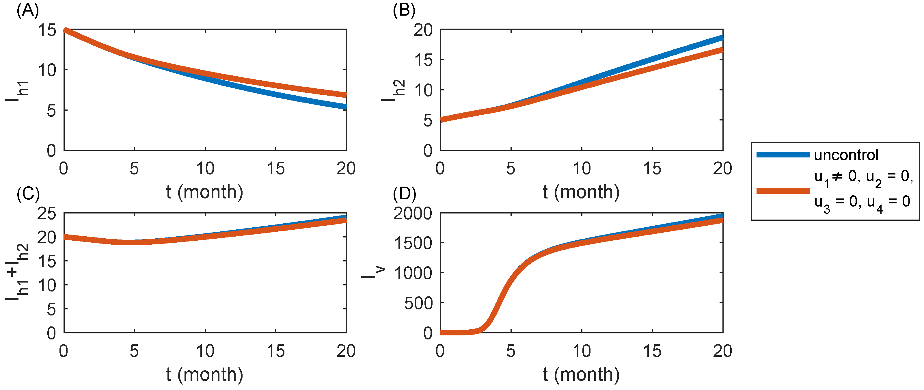
6.1. Strategy S1: Cultivating Disease-Free Seedlings Only ($u_1$)

For Strategy S1, $u_1$ is used to optimize the objective function J (given by (24)), while $u_2$, $u_3$ and $u_4$ are set to zero. From Figure 3, we can observe that there is no significant difference in the number of infected trees and ACPs in the case of “with and without control”, which implies that only cultivating disease-free seedlings does not effectively control the spread of citrus HLB.

6.2. Strategy S2: Injecting Nutrient Solution Only ($u_2$)

For Strategy S2, $u_2$ is used to optimize the objective function J, while we set $u_1$, $u_3$ and $u_4$ to zero. According to Figure 4A, it is clearly shown that the value of $I_{h2}$ decreases sharply, whereas $I_{h1}$ increases when the strategy S2 is applied. It follows from Figure 4D that the population of $I_v$ decreases when control is applied. The numerical results illustrate that applying Strategy S2 can lead to a reduction in the number of ACPs while increasing the number of infected citrus trees.

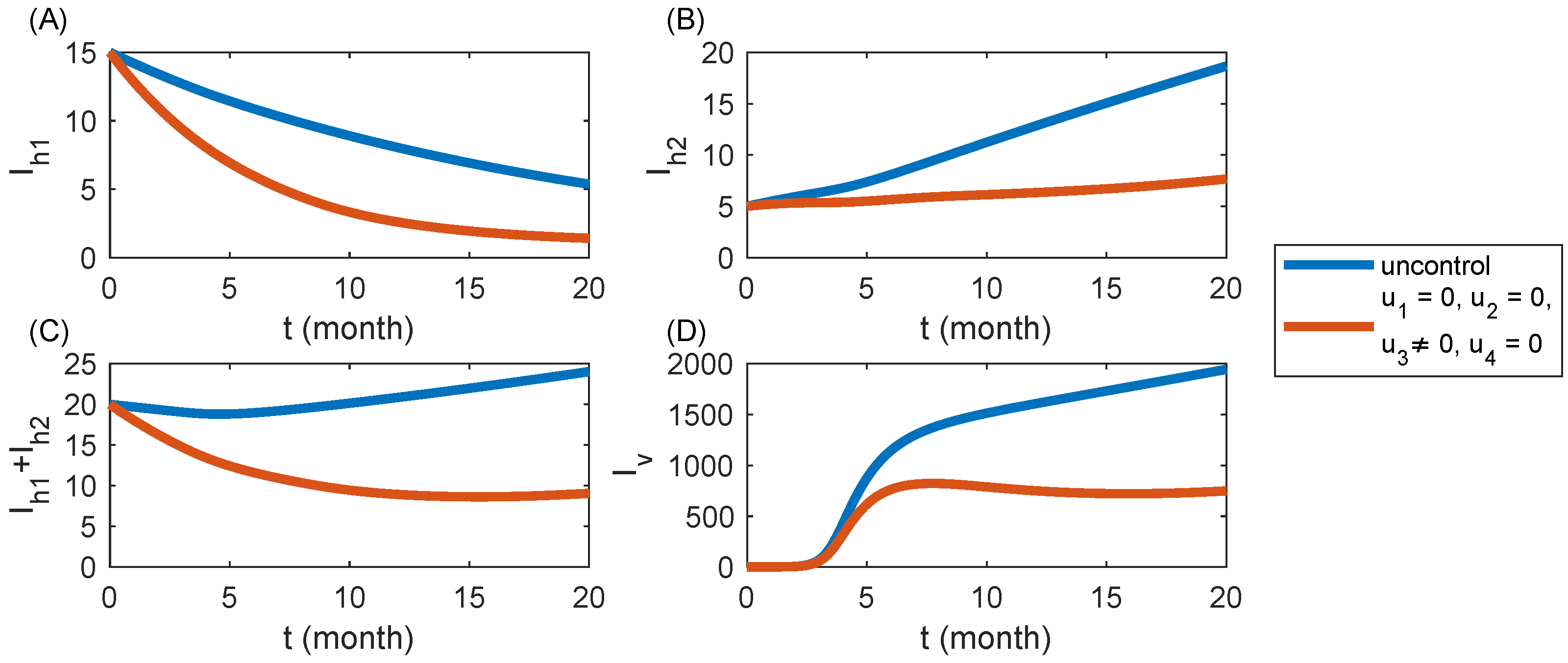
6.3. Strategy S3: Removal of Infected Trees Only ($u_3$)

For Strategy S3, $u_3$ is used to optimize the objective function J, while we set $u_1$, $u_2$ and $u_4$ to zero. Figure 5C,D reveal that the use of Strategy S3 helps to reduce the number of infected citrus trees and ACPs. It can also be seen that there exists a significant difference in the number of infected populations in the case of “with and without controls”, which implies that the removal of infected citrus trees is a very effective way to control the spread of the disease. This is because fewer infected hosts will lead to fewer infected vectors.

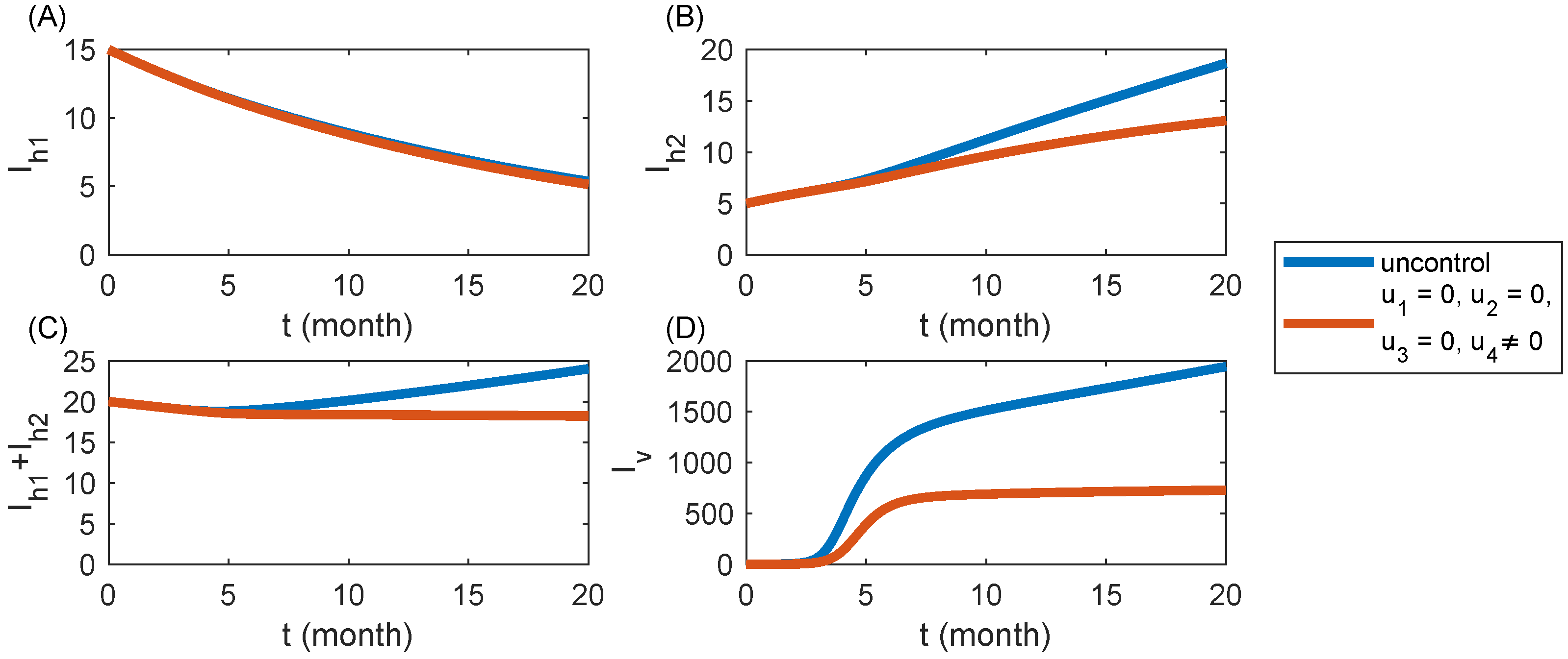
6.4. Strategy S4: Spraying Insecticides Only ($u_4$)

For Strategy S4, $u_4$ is used to optimize the objective function J, while we set $u_1$, $u_2$ and $u_3$ to zero. Similarly to what can be seen Strategy S3, we can observe through Figure 6 that there will be a significant decrease in the number of infected trees and ACPs in the presence of optimal spraying insecticides over time compared to the number of those without the control applied. Figure 3, Figure 4, Figure 5 and Figure 6 and

Table 3. Population of infected individuals at time $t_f$ and the objective functional in (24).

Strategy	${\mathit{I}}_{\mathit{h}1}\left({\mathit{t}}_{\mathit{f}}\right)$	${\mathit{I}}_{\mathit{h}2}\left({\mathit{t}}_{\mathit{f}}\right)$	${\mathit{I}}_{\mathit{v}}\left({\mathit{t}}_{\mathit{f}}\right)$	$\mathit{J}({\mathit{u}}_1,{\mathit{u}}_2,{\mathit{u}}_3,{\mathit{u}}_4)$
no control	5.3640	18.6695	1944.6712	357,680
S1	6.8321	16.6514	1877.4227	347,445
S2	10.0822	12.2697	1740.0477	329,633
S3	1.4065	7.6593	749.2521	217,770
S4	5.1447	13.0783	728.6598	199,738
S5	2.6188	4.9042	298.0053	132,131

indicate that insecticide spraying and the removal of infected trees are more effective prevention measures compared to the production of HLB-free nursery trees and nutrient solution treatment. This is consistent with the finding that the sensitivity (Figure 2) to parameters ${\mu }_v$ and ${\gamma }_2$ is significantly greater than that to $\alpha$, $\rho$ and $\nu$.

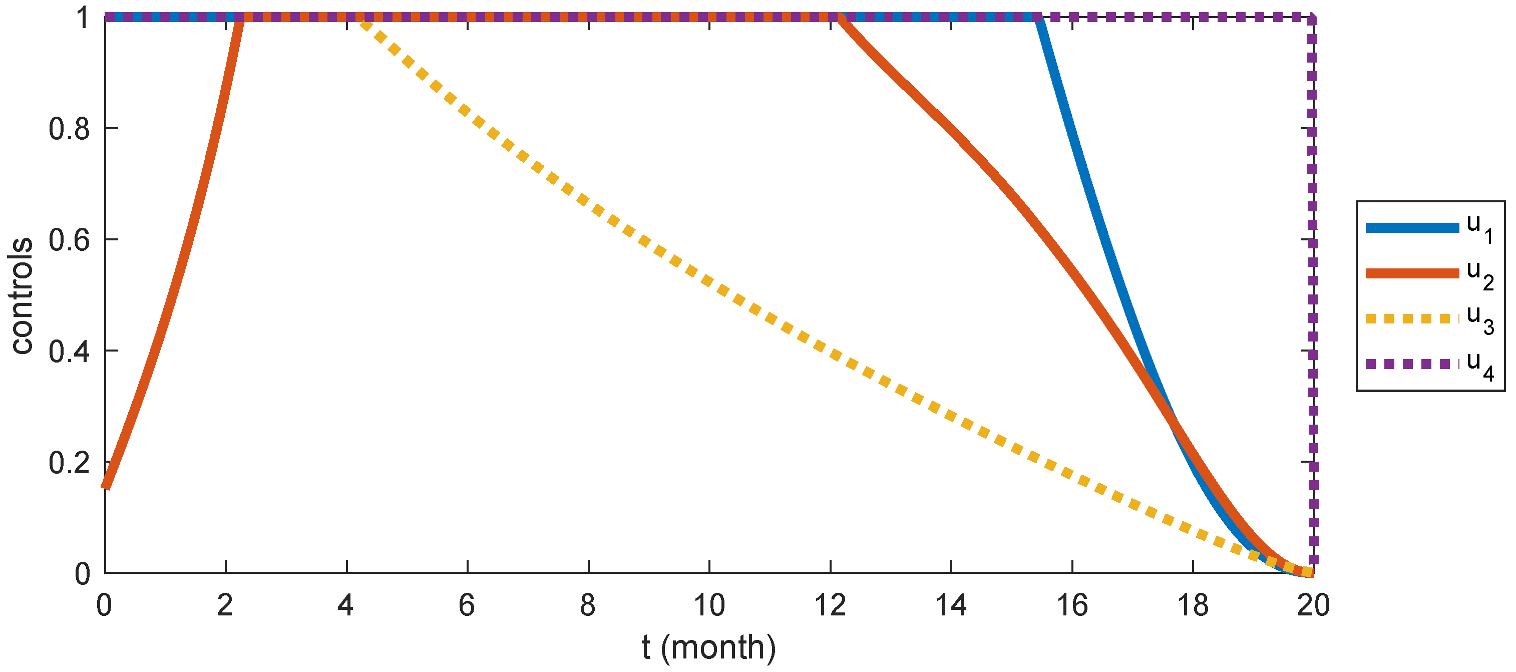
6.5. Strategy S5: Integrated Control ($u_1,u_2,u_3$ and $u_4$)

For Strategy S5, $u_1,u_2,u_3$ and $u_4$ are used to optimize the objective function in J. It can be seen from Figure 7 that the numbers of $I_{h1}$, $I_{h2}$ and $I_v$ are reduced considerably over time with the application of the optimal controls compared to the number of infected individuals in the absence of controls.

It is observed from Table 3 that the single prevention measure of spraying insecticides results in lower values compared to the removal of infected trees in terms of $I_v$ and the objective function J, while $I_{h1}$ and $I_{h2}$ exhibit the opposite trend. This indicates that removing infected trees and spraying insecticides each have specific advantages in controlling the populations of infected trees and infected psyllids, respectively. Therefore, combining these two strategies is a better choice. In summary, compared with single control strategies, the integrated control strategy, Strategy S5, is the most effective strategy.

The optimal control trajectories under different control measures are given in Figure 8. It can be seen that during the early phase of HLB outbreak, upper-bound control strategies should be adopted in most cases to suppress the transmission of the disease, except for the strategy of nutrient solution treatment.

7. Conclusions

In this paper, we extend the deterministic vector-borne model of HLB into an optimal control problem. We demonstrate the well posedness and biological meaningfulness of the proposed model (1) by establishing the existence, positivity, and boundedness of all solutions within the feasible region. We then compute the basic reproduction number, ${\mathcal{R}}_0$, using the next-generation matrix and analyze the stability of its equilibria. Our theoretical results indicate that the disease-free equilibrium is globally asymptotically stable when ${\mathcal{R}}_0<1$, whereas system (1) is persistent when ${\mathcal{R}}_0>1$.

We performed a sensitivity analysis of the basic reproductive number, ${\mathcal{R}}_0$, with respect to each parameter to identify the most sensitive ones. To address disease prevalence, we expanded the model into an optimal control framework incorporating four control measures: disease-free budwood and nursery tree production, nutrient solution application, removal of HLB-infected trees, and insecticide spraying. We computed the optimal control function by minimizing the number of infected trees and ACPs, while considering the cost of interventions. We then analytically examined the existence and characterization of the optimal controls. Using Pontryagin’s minimum principle, we derived the exact optimal control formula and the necessary conditions for the existence of the optimal control solution.

We conducted numerical simulations of our mathematical model using estimated and assumed parameter values, along with appropriate initial conditions. These simulations demonstrate the efficacy of the proposed control strategies. The key findings from our numerical simulations are as follows:

(i)

Upon eliminating the sensitivity analysis, it becomes evident that the primary parameters influencing the basic reproduction number (${\mathcal{R}}_0$) are the infection rates of citrus trees ($\beta$) and citrus psyllids ($\zeta$), the natural death rate of citrus psyllids (${\mu }_v$), the disease-induced mortality of citrus trees without nutrient solution treatment (${\gamma }_2$) and the maximum abundance of ACPs per tree (M);

(ii)

When compared to the production of disease-free budwood and nursery trees, as well as the application of nutrient solutions, the removal of HLB-infected trees and insecticide spraying prove to be more effective in minimizing the spread of HLB;

(iii)

Among the various strategies, the integrated control strategy, Strategy $S5$, emerges as the most effective.

In recent years, China has widely adopted three fundamental measures: the production of HLB-free nursery trees, prompt removal of HLB-infected trees, and large-scale collaborative prevention and control of ACPs [2]. The removal of infected trees typically occurs after trained inspector teams visually confirm HLB symptoms. However, this visual inspection process is not only time-consuming but also lacks sufficient accuracy. Due to delays in the removal of infected trees and the emergence of insecticide resistance among ACPs, many growers have resorted to nutritional injections to alleviate the symptoms of HLB-affected trees. Consequently, this study paves the way for the development of a delayed model by incorporating time delays associated with growers’ intervention behaviors and the latent period of the disease. Additionally, further investigation into insecticide resistance and vector host preferences, such as landing and feeding preferences, is highly recommended.

References

- Bové, J.M. Huanglongbing: A destructive, newly-emerging, century-old disease of citrus. J. Plant Pathol. 2006, 88, 7–37. [Google Scholar]
- Zhou, C. The status of citrus Huanglongbing in China. Trop. Plant Pathol. 2020, 45, 279–284. [Google Scholar] [CrossRef]
- Sawada, K. Citrus Likubing (pre-report). Taiwan Agric. Rep. 1913, 83, 903–914. (In Japanese) [Google Scholar]
- Reinking, O.A. Diseases of economic plants in southern China. Philipp. Agric. 1919, 8, 109–135. [Google Scholar]
- Hall, D.G.; Gottwald, T.R. Pest management practices aimed at curtailing citrus huanglongbing disease. Outlooks Pest Manag. 2011, 22, 189–192. [Google Scholar] [CrossRef]
- Jacobsen, K.; Stupiansky, J.; Pilyugin, S.S. Mathematical modeling of citrus groves infected by huanglongbing. Math. Biosci. Eng. 2013, 10, 705–728. [Google Scholar] [CrossRef] [PubMed]
- Grafton-Cardwell, E.E.; Stelinski, L.L.; Stansly, P.A. Biology and management of Asian citrus psyllid, vector of the huanglongbing pathogens. Annu. Rev. Entomol. 2013, 58, 413–432. [Google Scholar] [CrossRef]
- Alvarez, S.; Rohrig, E.; Solís, D.; Thomas, M.H. Citrus greening disease (Huanglongbing) in Florida: Economic impact, management and the potential for biological control. Agric. Res. 2016, 5, 109–118. [Google Scholar] [CrossRef]
- McManus, P.S.; Stockwell, V.O.; Sundin, G.W.; Jones, A.L. Antibiotic use in plant agriculture. Annu. Rev. Phytopathol. 2002, 40, 443–465. [Google Scholar] [CrossRef]
- Braga, G.A.; Ternes, G.; Uilamiu, R.G.D.; Castro, A.; Silva, M.V.; Laranjeira, F.F. Modelagem Mathemática da Dinâmica Temporal do HLB em Citros? In Proceedings of the VIII Congresso Brasileiro de Agroinformática, Bento Goncalves, Brazil, 17 October 2011; pp. 1–5. [Google Scholar]
- Chiyaka, C.; Singer, B.H.; Halbert, S.E.; Morris, J.G., Jr.; van Bruggen, A.H. Modeling huanglongbing transmission within a citrus tree. Proc. Natl. Acad. Sci. USA 2012, 109, 12213–12218. [Google Scholar] [CrossRef]
- Taylor, R.A.; Mordecai, E.A.; Gilligan, C.A.; Rohr, J.R.; Johnson, L.R. Mathematical models are a powerful method to understand and control the spread of Huanglongbing. PeerJ 2016, 4, e2642. [Google Scholar] [CrossRef] [PubMed]
- Guo, J.; Gao, S.; Yan, S.; Liao, Z. Bifurcation and optimal control analysis of delayed models for huanglongbing. Int. J. Biomath. 2022, 15, 2250049. [Google Scholar] [CrossRef]
- Liao, Z.; Gao, S.; Yan, S.; Zhou, G. Transmission dynamics and optimal control of a Huanglongbing model with time delay. Math. Biosci. Eng. 2021, 18, 4162–4192. [Google Scholar] [CrossRef]
- Zhang, F.; Qiu, Z.; Huang, A.; Zhao, X. Optimal control and cost-effectiveness analysis of a Huanglongbing model with comprehensive interventions. Appl. Math. Model. 2021, 90, 719–741. [Google Scholar] [CrossRef]
- Odionyenma, U.B.; Omame, A.; Ukanwoke, N.O.; Nometa, I. Optimal control of Chlamydia model with vaccination. Int. J. Dyn. Control 2022, 10, 332–348. [Google Scholar] [CrossRef]
- Jan, M.N.; Zaman, G.; Ali, N.; Ahmad, I.; Shah, Z. Optimal control application to the epidemiology of HBV and HCV co-infection. Int. J. Biomath. 2022, 15, 2150101. [Google Scholar] [CrossRef]
- Kumar, A.; Gupta, A.; Dubey, U.S.; Dubey, B. Stability and bifurcation analysis of an infectious disease model with different optimal control strategies. Math. Comput. Simul. 2023, 213, 78–114. [Google Scholar] [CrossRef]
- Asamoah, J.K.K.; Safianu, B.; Afrifa, E.; Obeng, B.; Seidu, B.; Wireko, F.A.; Sun, G.Q. Optimal control dynamics of Gonorrhea in a structured population. Heliyon 2023, 9, e20531. [Google Scholar] [CrossRef]
- Tu, Y.; Gao, S.; Liu, Y.; Chen, D.; Xu, Y. Transmission dynamics and optimal control of stage-structured HLB model. Math. Biosci. Eng. 2019, 16, 5180–5205. [Google Scholar] [CrossRef]
- Zhou, X.; Qi, G. Population dynamics of Diaphorina citri Kuwayama in different types of citrus orchards in Fogang County, Guangdong Province. J. Biosaf. 2019, 28, 249–253. (In Chinese) [Google Scholar]
- Deng, M. Forming process and basis and technological points of the theory emphasis on control citrus psylla for integrated control Huanglongbing. Chin. Agric. Sci. Bull. 2009, 25, 358–363. [Google Scholar]
- Van der Merwe, C. The Citrus Psylla (Trioza merwei, Pettey). J. Dept. Agric. 1923, 7, 135–141. Available online: https://hdl.handle.net/10520/AJA0000020_1462 (accessed on 22 August 2024).
- Zhang, M.; Powell, C.A.; Zhou, L.; He, Z.; Stover, E.; Duan, Y. Chemical compounds effective against the citrus Huanglongbing bacterium ‘Candidatus Liberibacter asiaticus’ in planta. Phytopathology 2011, 101, 1097–1103. [Google Scholar] [CrossRef]
- Liu, Y.H.; Tsai, J.H. Effects of temperature on biology and life table parameters of the Asian citrus psyllid, Diaphorina citri Kuwayama (Homoptera: Psyllidae). Ann. Appl. Biol. 2000, 137, 201–206. [Google Scholar] [CrossRef]
- Zhang, M.; Guo, Y.; Powell, C.A.; Doud, M.S.; Yang, C.; Duan, Y. Effective antibiotics against ‘Candidatus Liberibacter asiaticus’ in HLB-affected citrus plants identified via the graft-based evaluation. PLoS ONE 2014, 9, e111032. [Google Scholar] [CrossRef]
- Van den Driessche, P.; Watmough, J. Reproduction numbers and sub-threshold endemic equilibria for compartmental models of disease transmission. Math. Biosci. 2002, 180, 29–48. [Google Scholar] [CrossRef]
- Thieme, H.R. Convergence results and a Poincaré-Bendixson trichotomy for asymptotically autonomous differential equations. J. Math. Biol. 1992, 30, 755–763. [Google Scholar] [CrossRef]
- Xu, D.; Zhao, X.Q. Dynamics in a periodic competitive model with stage structure. J. Math. Anal. Appl. 2005, 311, 417–438. [Google Scholar] [CrossRef]
- Zhao, X.Q. Dynamical Systems in Population Biology; Springer: New York, NY, USA, 2003; Volume 16. [Google Scholar] [CrossRef]
- Chitnis, N.; Hyman, J.M.; Cushing, J.M. Determining important parameters in the spread of malaria through the sensitivity analysis of a mathematical model. Bull. Math. Biol. 2008, 70, 1272–1296. [Google Scholar] [CrossRef]
- Agusto, F.B.; Khan, M. Optimal control strategies for dengue transmission in Pakistan. Math. Biosci. 2018, 305, 102–121. [Google Scholar] [CrossRef]
- Xue, L.; Ren, X.; Magpantay, F.; Sun, W.; Zhu, H. Optimal control of mitigation strategies for dengue virus transmission. Bull. Math. Biol. 2021, 83, 8. [Google Scholar] [CrossRef] [PubMed]
- Sanchez, M.A.; Blower, S.M. Uncertainty and sensitivity analysis of the basic reproductive rate: Tuberculosis as an example. Am. J. Epidemiol. 1997, 145, 1127–1137. [Google Scholar] [CrossRef]
- Marino, S.; Hogue, I.B.; Ray, C.J.; Kirschner, D.E. A methodology for performing global uncertainty and sensitivity analysis in systems biology. J. Theor. Biol. 2008, 254, 178–196. [Google Scholar] [CrossRef] [PubMed]
- Helton, J.C.; Johnson, J.D.; Sallaberry, C.J.; Storlie, C.B. Survey of sampling-based methods for uncertainty and sensitivity analysis. Reliab. Eng. Syst. Saf. 2006, 91, 1175–1209. [Google Scholar] [CrossRef]
- Kar, T.K.; Batabyal, A. Stability analysis and optimal control of an SIR epidemic model with vaccination. Biosystems 2011, 104, 127–135. [Google Scholar] [CrossRef]
- Pang, L.; Ruan, S.; Liu, S.; Zhao, Z.; Zhang, X. Transmission dynamics and optimal control of measles epidemics. Appl. Math. Comput. 2015, 256, 131–147. [Google Scholar] [CrossRef]
- Fleming, W.H.; Rishel, R.W. Deterministic and Stochastic Optimal Control; Springer Science & Business Media: New York, NY, USA, 1975. [Google Scholar] [CrossRef]
- Lenhart, S.; Workman, J.T. Optimal Control Applied to Biological Models; Mathematical and Computational Biology Series; Chapman & Hall/CRC Press: London, UK, 2007. [Google Scholar]