Abstract
Graph neural networks (GNNs) have been highly successful in graph representation learning. The goal of GNNs is to enrich node representations by aggregating information from neighboring nodes. Much work has attempted to improve the quality of aggregation by introducing a variety of graph information with representational capabilities. The class of GNNs that improves the quality of aggregation by encoding graph information with representational capabilities into the weights of neighboring nodes through different learnable transformation structures (LTSs) are referred to as implicit GNNs. However, we argue that LTSs only transform graph information into the weights of neighboring nodes in the direction that minimizes the loss function during the learning process and does not actually utilize the effective properties of graph information, a phenomenon that we refer to as graph information vanishing (GIV). To validate this point, we perform thousands of experiments on seven node classification benchmark datasets. We first replace the graph information utilized by five implicit GNNs with random values and surprisingly observe that the variation range of accuracies is less than ± 0.3%. Then, we quantitatively characterize the similarity of the weights generated from graph information and random values by cosine similarity, and the cosine similarities are greater than 0.99. The empirical experiments show that graph information is equivalent to initializing the input of LTSs. We believe that graph information as an additional supervised signal to constrain the training of GNNs can effectively solve GIV. Here, we propose GinfoNN, which utilizes both labels and discrete graph curvature as supervised signals to jointly constrain the training of the model. The experimental results show that the classification accuracies of GinfoNN improve by two percentage points over baselines on large and dense datasets.
MSC:
68-XX
1. Introduction
Graph neural networks (GNNs) have achieved great success on a wide range of graph analysis tasks, such as recommender systems [1,2], traffic flow prediction [3,4], and biochemistry research [5,6]. The success of GNNs is mainly attributed to adaptively enriching the representations of target nodes by aggregating the features of neighboring nodes in a supervised learning paradigm, which can be summarized as the message-passing neural network framework (MPNN) [7]. The MPNN generates node representations by iteratively transforming, aggregating, and updating the features of neighboring nodes. The transformation and update operations usually correspond to linear transformations and nonlinear activation functions, respectively, while the aggregation operation is more complex and valuable. The aggregation operation involves two main aspects: defining the neighboring nodes and measuring the importance of the neighboring nodes. Many works designed GNNs that simply utilized the nodes directly connected to the target node as the neighboring nodes [8,9,10], and other designs employed the acquisition of neighboring nodes by random walk in order to explore rich and diverse local topologies [11,12]. There are usually three ways to define the weights of neighboring nodes: (1) consider the importance of all neighboring nodes as equal [5,10,13], (2) use node degree to assign the importance of neighboring nodes [8], and (3) assign the importance of neighboring nodes implicitly in a data-driven manner [9,14].
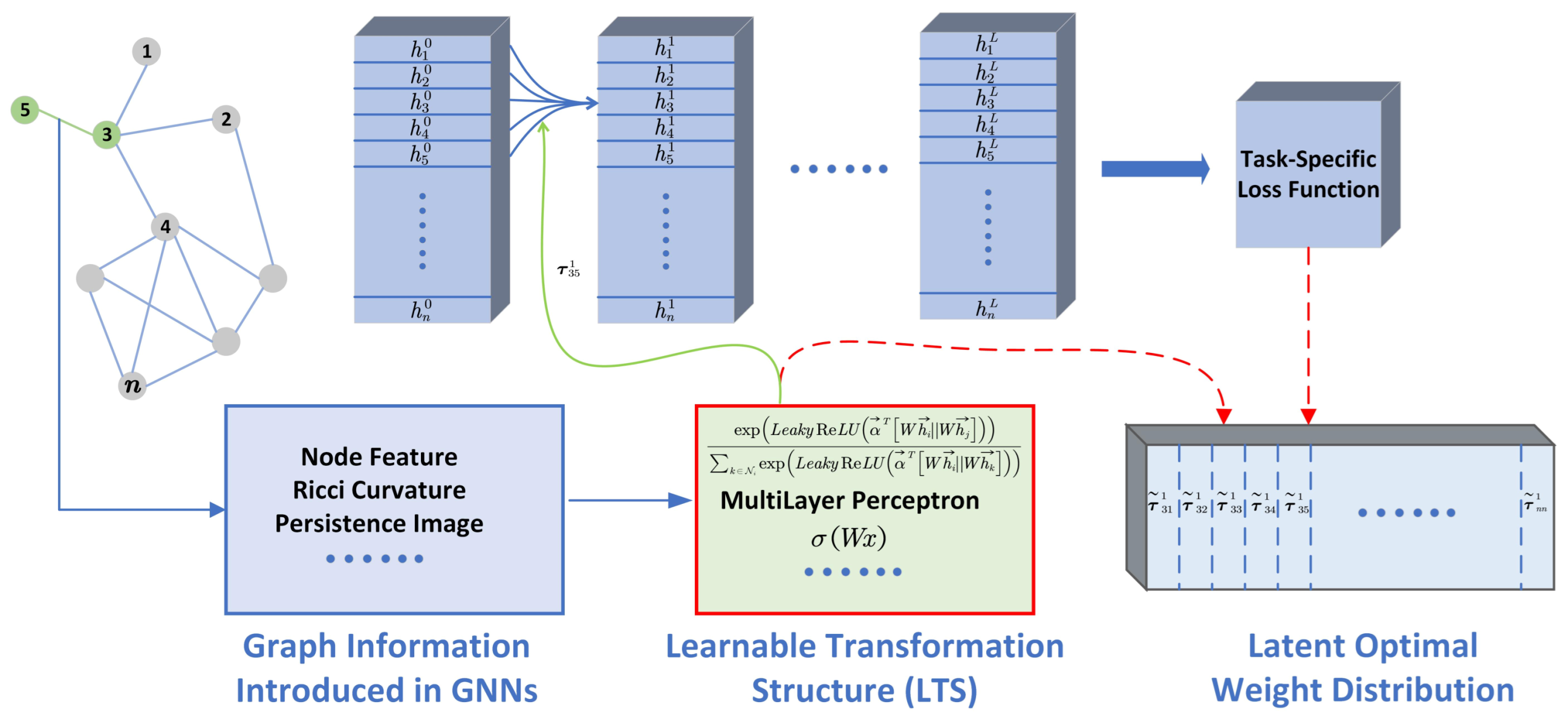
The weights of neighboring nodes that are implicitly generated can adapt datasets automatically. We refer to GNNs adopting this scheme as implicit GNNs. We reorganize the pipeline of generating the weights of implicit GNNs into three parts: (1) the graph information, (2) the learnable transformation structures (LTSs), and (3) the weights of neighboring nodes, as shown in Figure 1. The graph information is the input of the LTS, and the weights of neighboring nodes are the output. For example, CurvGN [14] takes advantage of the Ricci curvature [15] and the multilayer perceptron (MLP) to generate the weights.
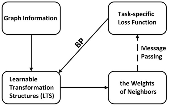
Figure 1.
An illustration of the forward propagation pipeline of LTSs in implicit GNNs. BP means backward gradient propagation.
In general, the weights generated by implicit GNNs are not only adaptive to datasets but also take advantage of the valuable properties of graph information to enhance the quality of node representations. However, we argue that the LTSs only transform graph information into the weights of neighboring nodes in the direction that minimizes the loss function during training and does not utilize the unique properties of graph information, a phenomenon that we refer to as graph information vanishing (GIV). To validate this point, we select five implicit GNNs, CurvGN, PEGN [16], GAT, HGCN [17] and AGNN [18], and conduct thousands of experiments on 7 node classification datasets. First, we replace the graph information with the random values obtained by sampling from a 0–1 uniform distribution. Surprisingly, we observe that the variation range of classification accuracies is less than ± 0.3%. Then, we visualize these two types of weights, the difference between which is difficult to visually perceive. Moreover, we quantitatively characterize the similarity of the weights generated from graph information and random values by cosine similarity. The cosine similarities are greater than 0.99 under most conditions. The experimental results indicate that the weights generated by the LTSs do not retain the valuable properties of graph information, i.e., the mechanism of implicit GNNs cannot properly utilize graph information.
We argue that GIV is triggered by the fact that the loss function is task-specific and not associated with graph information. Assuming the existence of latent optimal weights that minimize the task-specific loss, the goal of the LTSs is simply to update the learnable parameters by back propagation so that the learned weights are as close to the latent optimal weights as possible. If the fitting ability of the LTSs is strong enough, the input can be arbitrary in theory. Since the loss function is independent of the graph information, the weights generated by the LTSs naturally do not retain the properties of graph information.
We also believe that graph information characterizing datasets is essential to improve the performance of GNNs. According to the above analysis, GIV is caused by the lack of connection between the loss function and graph information. Intuitively, graph information can also be used as an auxiliary supervised signal to constrain the training of GNNs, thus effectively utilizing graph information to enrich the knowledge of GNNs. Inspired by joint learning [6], we propose GinfoNN, which is able to utilize both supervised signals provided by labels and auxiliary supervised signals provided by graph information. GinfoNN decomposes GNNs into two parts, a feature extractor and a task-specific head, while adding a task–auxiliary head. The task-specific head and task–auxiliary head correspond to task-specific loss based on the labels and task–auxiliary loss based on graph information, respectively. In particular, we take the discrete graph curvature [14,19] as an auxiliary supervised signal that quantifies the structural connectivity of node pairs. Experimental results show that GinfoNN outperforms the baselines on large and dense datasets. The ablation experiments also demonstrate the necessity of the discrete graph curvature for improving the performance of GNNs.
The remainder of this paper is organized as follows. In Section 3, we review the pipeline of implicit GNNs for computing the weights of neighboring nodes, rederive five implicit GNNs, and illustrate GIV through empirical experiments. In Section 4, we describe the framework GinfoNN and the discrete graph curvature in detail. In Section 5, we evaluate the performance of GinfoNN on node classification benchmark datasets. In Section 2, we briefly review the related work. Finally, Section 6 discusses several inspiring issues related to this work, and Section 7 concludes the paper.
2. Related Work
GNNs. GNNs can be divided into spectral GNNs and spatial GNNs. The initial concept of convolution on the graph [20] is defined based on the spectral graph theory. This method cannot design spatially localized filters and needs intense computations due to the matrix eigendecomposition. In order to avoid computing the eigendecomposition of the graph Laplacian matrix, a truncated expansion of Chebyshev polynomials is employed to approximate the filter [21]. GCN [8] further simplifies the filter by fixing the polynomials to 1 and using a renormalization trick. Since spectral GNNs focus on specific graphs, they face many insurmountable limitations, such as the inability of trained models to generalize to other graphs, which can be handled well by spatial GNNs. Spatial filters can directly work on the local structure of graphs, and different filters can be designed for nodes with different-sized neighbors [5]. MoNet [22] proposes a mixture model to successfully adapt CNN for the non-Euclidean domain and generalize some previous models. GraphSAGE [10] samples fixed-size neighbors as receptive fields and uses different methods to aggregate their representations. To assign specific weights for neighborhood nodes, GAT [9] incorporates the self-attention mechanism into graph convolution. CurvGN [14] and PEGN [16] introduced the Ricci curvature and persistence images as additional knowledge to assign specific weights to channels of node features, respectively. With the exploration of the connection between GNN and the diffusion model, diffusion-based GNNs open a new path to improving GNNs. HiD-Net [23] proposes a new general diffusion framework for unifying GNNs and shows effectiveness on both homophily and heterophily graphs.
Theoretical analysis. GNNs, as black-box models, arouse wide concern about their power and limits. The mechanism and oversmoothing problem of GCN are explored and explained by considering the convolution layer as symmetric Laplacian smoothing [24]. A theoretical framework is proposed for analyzing the discriminative power of GNNs to distinguish different graph structures [13]. The expressive power of GCNs with deeper layers is investigated, and a weight normalization strategy is proposed to improve their expressive power [25]. The expressive power of GNNs for Boolean node classification is further analyzed, and adding readout functions acts as an efficient way to increase logical expressiveness [26]. The explanation of GNNs is also investigated systematically [27]. Besides, some methods contribute to modifying network architectures to improve the performance of GNNs. SGC [28] simplifies graph convolutional networks to adapt large-scale graphs by removing nonlinearities weight matrices. Deepgcns [29] expands the layers of GCN from 2 to 56 layers by referring to the concept of residual/dense connections in CNN. For the graph classification task, the effect of attention on the readout phase is analyzed, and a weakly supervised method is proposed to train attention [30]. Note that the most of analysis works focus on GCN and its variants, which are regarded as explicit GNNs in this paper. By contrast, the analysis of implicit GNNs is not nearly enough.
Joint learning. Joint learning aims at enriching the supervision signals by utilizing various attributive and topological graph information. Utilizing attributive information to generate pseudo labels can boost the adversarial robustness of GNNs [31]. M3S [32] proposes a multistage joint-training mechanism by using the K-means clustering algorithm. PairwiseDistance [33] regards the shortest distance between two nodes as the auxiliary supervision signal. Centrality Score Ranking [34] recovers the relative order of centrality scores between pairwise nodes as the auxiliary task. GPN [35] develops a bilevel optimization framework to simultaneously optimize the graph generator and the downstream predictor. Implementing an adversarial solution in the joint learning paradigm can learn causal independence and achieve graph out-of-distribution generalization [36]. Joint learning has been shown to improve the performance and adversarial robustness of GNNs by exploiting valuable graph information, which can actually utilize graph information and solve GIV naturally.
3. Implicit GNNs
3.1. Implicit GNNs: A Unified View
In this section, we first summarize several key components of GNNs and further sort out the pipeline for implicit GNNs to compute the weights of neighboring nodes.
Key components of GNNs. GNNs consist of a message-passing phase and a readout phase in the message-passing neural network framework (MPNN) [7]. The message-passing phase is on the node level, while the readout phase is on the graph level. We only focus on the message-passing phase, on which the weights of neighboring nodes have a significant effect. In general, the forward propagation formula for message passing can be summarized as
where is the representation of the node i on the layer, F indicates the dimension of the node feature, is the feature of the edge from node i to node j, D indicates the dimension of the edge feature, is the neighboring nodes of node i, and are differentiable functions, and □ is a differentiable, permutation-invariant aggregation function, e.g., sum, mean, or max.
where is the activation function, W is a matrix of filter parameters, is the weight of the node feature from node j to node i, and is a transformation function.
The forward propagation formulas of mostly spatial GNNs can be simplified for the aggregation part and the reweight part. The corresponding formulas are Equation (2) and Equation (3), respectively. If needs to be learned, such as MLP, the GNN is referred to as an implicit GNN; otherwise, it is referred to as an explicit GNN. In other words, we classify GNNs as explicit GNNs or implicit GNNs according to whether the weights of neighbors need to be learned.
The pipeline of generating the weights for implicit GNNs. For implicit GNNs, edge feature is interpreted as graph information, which helps to assign the weights of neighbors in aggregation, and is referred to as the learnable transformation structure (LTS). A common assumption behind implicit GNNs is that can help GNNs by learning more knowledge about datasets, and the LTS ensures that automatically adapts datasets in a data-driven manner. The pipeline of implicit GNNs is shown in Figure 2, and the role of LTS is illustrated at the bottom of Figure 2. Some popular GNNs, such as CurvGN, PEGN, GAT, HGCN, and AGNN, can be rederived into the pipeline. The benefit of this protocol is to help us unify the analysis and the understanding of GIV for implicit GNNs. The graph information and the corresponding LTSs utilized by these five models are shown in Table 1.

Figure 2.
A pipeline of implicit GNNs. The top part of the figure is the aggregation of GNNs, while the bottom part of the figure is the reweight part. Given the dataset and the network architecture, we assume the task-specific loss function forces the LTSs to learn the latently optimal weight distribution during training.

Table 1.
Summary of graph information and LTS for the five implicit GNNs.
3.1.1. Special Case 1
When utilizing the CurvGN model, it is assumed that the Ricci curvature can endow GNNs with more discriminative power. The Ricci curvature is a measure whose result indicates whether the structural relationship between a pair of nodes is tight or alienated. The neighbors of pairwise nodes in the same community often have many shortcuts and largely overlap. If the Ricci curvature of edges connecting two communities is positive, then information should be easily exchanged between the corresponding nodes, and if this is negative, then information is not easily exchanged between the corresponding nodes.
The Ricci curvature is the graph information of CurvGN, and the two-layer MLP is the LTS. The formula of the reweight part is
where represents an individual normalization for each channel of the node features. The dimension of is set to the same as . Therefore, can give separate weights to each channel of the node features to make the model more discriminative. The aggregation part of CurvGN is formulated as
3.1.2. Special Case 2
PEGN argues that local structural information of graphs can improve the adaptability of GNNs to large graphs with heterogeneous topology. PEGN uses persistence homology, a principled mathematical tool, to describe the loopiness of nodes’ neighbors, which measures the information transmission efficiency of each node. PEGN utilizes persistence images to quantitatively characterize the persistence homology of each edge.
PEGN refers to persistent images of graphs as graph information. The reweight part and aggregation part of PEGN is the same as that of CurvGN. PEGN also selects a two-layer MLP as the LTS of the model.
3.1.3. Special Case 3
GAT aims to address the limitations of spectral GNNs by implicitly computing the weights of neighboring nodes. GAT introduces the self-attention mechanism to automatically transform the hidden representation of nodes into the attention coefficients which are treated as weights of neighbors.
The graph information introduced by GAT is the vector that concatenates the hidden features of pair-wise nodes , and represents the concatenation operation. The formula of GAT’s reweight part is
where the weight matrix and the weight vector are shared by all information. The LTS of GAT is . To ensure the stability of training, GAT also utilizes a K-head attention mechanism. The formula of the aggregation part is given by
3.1.4. Special Case 4
HGCN extends GNNs from Euclidean space to hyperbolic space and aims to solve the distorted deformation when graphs are hierarchical or scale-independent in Euclidean space. HGCN first maps node features to the hyperboloid manifold by exponential mapping and then maps node features in the hyperboloid space to the tangent space by logarithmic mapping. Since the tangent space is Euclidean and isomorphic to , the whole computation of the aggregation part is in the tangent space. The output generated by aggregation is then mapped to the hyperbolic space by an exponential mapping. Finally, HGCN implements GNN in hyperbolic space.
HGCN takes the concatenated vector of hidden features of two nodes on the edge in the tangent space as graph information , where K denotes the hyperbolic curvature. To transform graph information as the weight of node features, MLP is used as the LTS. So, the formula of the reweight part is
where is the weight of node j to node i. The formula of the aggregation part is
Note that some operations, such as the activation function in hyperbolic space, are omitted to highlight the core of HGCN. For more details, please see [17].
3.1.5. Special Case 5
AGNN is a special kind of GNN, which does not use the weight matrix to transform the node features in the aggregation process but only uses the attention propagation matrix to aggregate the node features. The attention propagation matrix is generated by a special attention mechanism in a data-driven mode. AGNNs argue that the mechanism is able to gain more accurate predictions by learning the dynamic and adaptive weights of neighbors.
The AGNN uses the cosine of the hidden features of the two nodes on the edge as graph information , and . Then, the attention mechanism of AGNN is the reweight part, which is calculated as
where is a learnable scalar, which is the TLS of the AGNN. If node i and node j are not connected, the corresponding value of the attention propagation matrix is 0. Therefore, the formula of the aggregation can be rewritten as
3.2. Graph Information Vanishing of Implicit GNNs
3.2.1. The Effect of Random Values Substituting Graph Information
We explore the impact of replacing graph information with random values on implicit GNNs. See Section 5.1 for more information on the datasets. To avoid randomness and ensure reproducibility, we select three random seeds, which are 0, 10, 100. Then, we randomly sample from a 0–1 uniform distribution and replace the generated random values with graph information, with the corresponding models being model_0, model_10, and model_100, respectively. We compare the classification accuracies of the five implicit GNNs and their corresponding random-value substituting models on seven benchmark datasets, as shown in Table 2. Experimental results suggest that replacing graph information with random values causes almost no performance degradation of implicit GNNs. The best results on different datasets are distributed between implicit GNNs and implicit GNNs with random values among the five sets of models. Note that the difference in accuracies between implicit GNNs and implicit GNNs with random values is small and less than 0.3 percent on most datasets. It illustrates that replacing the graph information with random values has almost no impact on the performance of implicit GNNs. For the LTS, the roles of graph information and random values appear to be equivalent, i.e., to provide the initialization input of the LTS.
Table 2.
Summary of statistic results in terms of comparing different implicit GNNs with the corresponding GNNs with random values on seven benchmark datasets. OOM means out of memory.
On large and dense datasets, the accuracies of the AGNN are slightly better than that of AGNN_*. The reason is that the LTS of the AGNN is a learnable parameter that only exponentially scales up or down the cosine values between neighboring nodes. Due to the smoothing capability of GNNs, the node features tend to be similar and their corresponding cosine values are relatively large when a pair of nodes shares more neighboring nodes. The cosine operation slightly enhances the discriminative power of the model when the transformation power of LTS is insufficient. However, we also notice that the transformation ability of LTS of AGNN is too weak, resulting in the accuracies on large and dense datasets being much lower than that of other models with strong transformation ability of LTS. If we change the LTS to a self-attention mechanism, i.e., change the AGNN to GAT, replacing graph information with random values will have almost no impact on the performance of implicit GNNs.
We note that no particular implicit GNNs perform optimally on all datasets. It suggests that the possible direction to improve the performance of the GNN models may be to explore novel network architecture with better generalization capability rather than introducing different types of graph information as the input of LTS.
3.2.2. Similarity of Weights of Neighbors
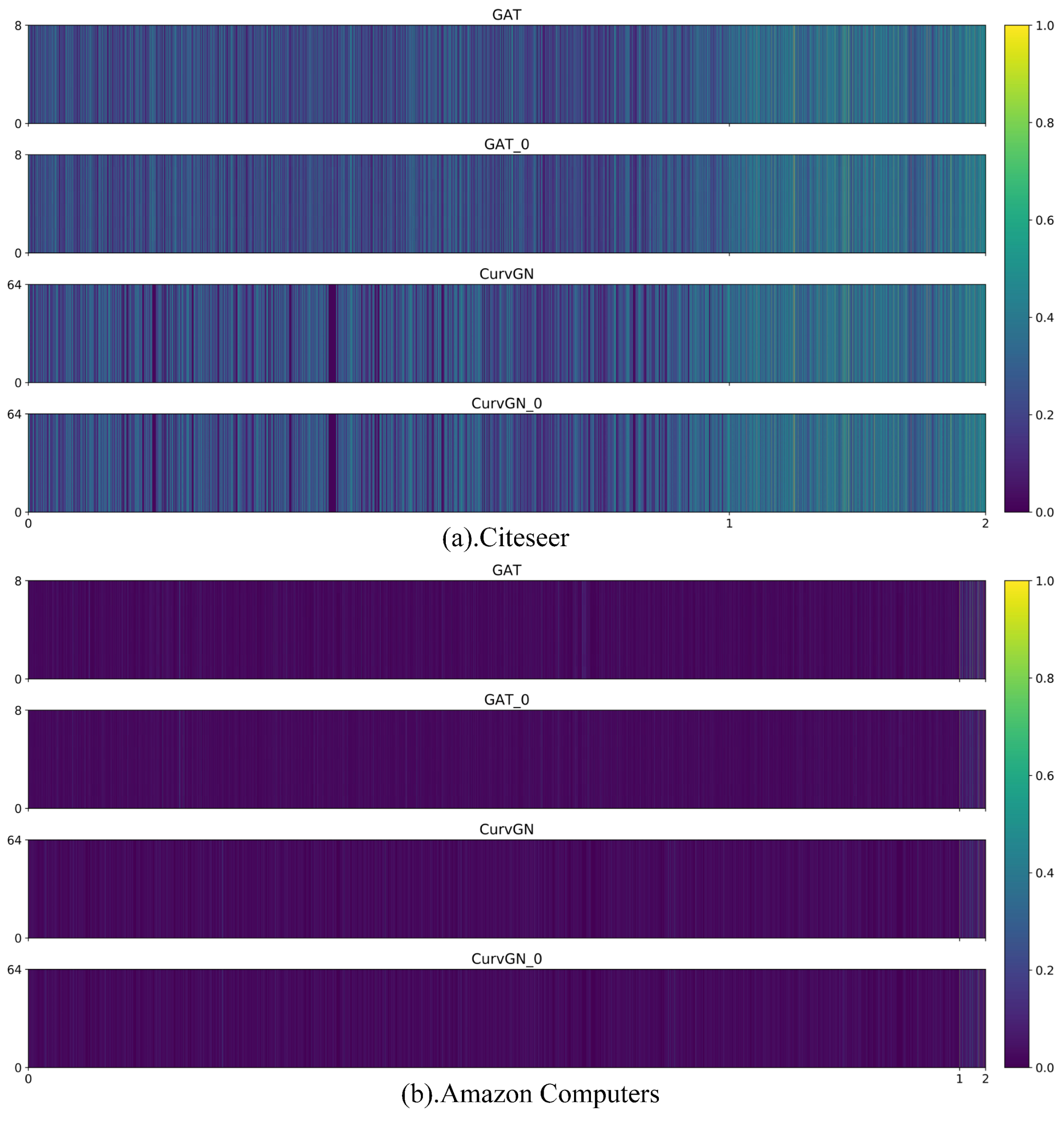
We qualitatively and quantitatively show that the weights of neighboring nodes obtained from the random values models are highly similar to those obtained from the original models. Without loss of generality, we select GATs and CurvGNs for detailed analysis. Figure 3 visualizes the weights of neighbors of GAT, GAT_0, CurvGN, and CurvGN_0 in the first layer on different datasets. Note that Citeseer is a relatively sparse and small dataset, and Computer is a relatively dense and large dataset. Regardless of the structure of the graphs, we hardly perceive the difference in the weights of neighbors between GAT and GAT_0 with our eyes. The phenomenon is also present on CurvGN. Due to the different network architectures between GAT and CurvGN, there are some small observable differences in their weights of neighbors. It qualitatively illustrates that even taking completely different graph information, LTS has the ability to transform it into highly similar weights of neighboring nodes.
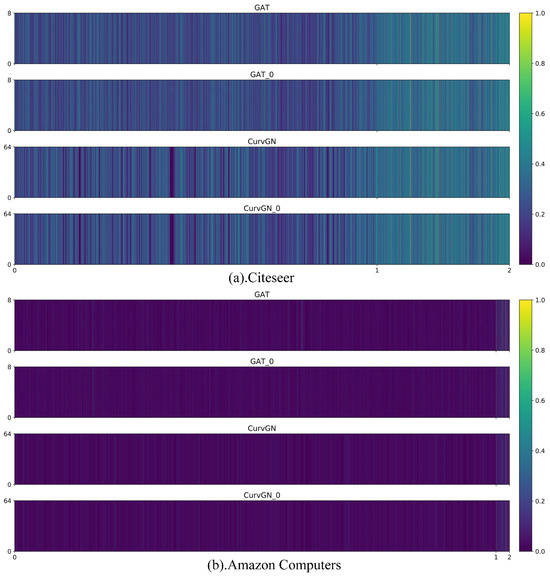
Figure 3.
An illustration of visualization of hidden layer’s weights of neighbors for different models on different datasets: (a) Weights of neighbors on Citeseer and (b) weights of neighbors on Amazon Computers. The vertical axis of each subgraph represents the dimension of the weights of neighbors. The horizontal axis of the subgraph is divided into two parts, where 0 to 1 represents the weights of edges, and 1 to 2 represents the weights of self-loops.
We quantitatively characterize the similarity of weights of neighbors through the cosine similarity. Since the weights of neighboring nodes may be a matrix, we first need to reduce the dimensionality from matrix form to vector form. We observe that there is almost no difference in the colors of the same column of Figure 3, which indicates that the difference in the values of the weights in different channels is very small. Further, we quantitatively measure the average variation in the weights across channels using
where A indicates the weights of neighboring nodes, m is the dimension of A, n is the number of edges. The above formula actually measures the average absolute difference between the values of different channels compared with the mean values. The average absolute difference in hidden layers’ weights for different models on benchmark datasets is shown in Table 3. We found that the average absolute difference in weights of different channels is quite small and can be negligible. Therefore, we use averaging over channels to reduce the weights of neighbors in matrix form to vector form and then compute the cosine similarity to compare the similarity of different weights. The formula of the cosine similarity is shown as
Table 3.
Summary of consistency of hidden layers’ weights of neighbors for different models.
We select cosine similarity to quantify the high similarity of the weights of neighboring nodes generated by graph information and random values, as shown in Table 4. For GAT, CurvGN, and PEGN, Table 4 shows that the cosine similarity of the weights exceeds 0.99 in most cases. We notice a small decrease in the similarity of the weights for GAT on Coauthor CS and Coauthor Physics. The reason is that GAT uses 128-dimensional vectors as graph information and the LTS has insufficient learning ability on relatively large and dense datasets. Highly similar weights of neighbors illustrate that replacing graph information with random values has almost no effect on implicit and also explains the results of Table 2 and Figure 3. A large number of experiments confirm the existence of GIV for implicit GNNs.
Table 4.
Summary of cosine similarity of hidden layer’s weights of neighbors for LTS with different graph information. Keep 4 decimal places and round off the rest.
4. Ginfonn: Graph Curvature Boosts GNNs
In this section, we first detail a kind of graph information that characterizes the structural relationship of pairwise nodes, the Ricci curvature, which is the same as the graph information utilized by CurvGN. Inspired by Joint Training [33], we develop GinfoNN, which effectively exploits the Ricci curvature by treating it as an auxiliary supervised signal. This way inherently solves GIV, which means that GinfoNN exactly makes use of graph information.
4.1. The Ricci Curvature
Curvature is able to qualitatively measure the degree of curvature in space. In Euclidean space, curvature measures the degree to which a curve deviates from a straight line, or a surface deviates from a plane. In Riemannian geometry, curvature measures the degree to which a local manifold deviates from Euclidean space, and Ricci curvature portrays its deviation in the orthogonal direction. Ollivier et al. [19] generalize the Ricci curvature from continuous space to discrete space by means of optimal transport theory, e.g., graph.
The Ricci curvature on the graph measures the extent of overlap or connection of pairwise nodes to neighboring nodes. The Ricci curvature treats the target node i and its neighboring nodes as a kind of probability distribution . We consider any probability distribution as an object of mass 1. Now, we want to know the minimum average mass-preserving transportation plan for transferring the mass of to , known as the Wasserstein distance . Naturally, the larger the Wasserstein distance of a pair of nodes, the weaker the connection between the two nodes, and vice versa. Besides, the Ricci curvature also takes the shortest distance between two nodes into account. The Ricci curvature of an edge can be formulated as
We choose a simple and effective probability distribution with a hyperparameter , as in [15]. Following the existing work [37], we set . For an undirected and unweighted graph , the probability distribution of the node j with degree k can be
The Ricci curvature contains a wealth of local structural information from the perspective of graph theory. In general, we consider the (infinitely extended) grid as a plane on the graph, and all its nodes are structurally equivalent. The Ricci curvature, on the other hand, portrays the direction and degree of deviation of the local structure with respect to the grid. If the curvature is negative, the neighboring nodes of these two nodes tend to be separated. If the curvature on the edges is positive, it indicates that these two nodes are relatively closely connected structurally, as their neighboring nodes tend to converge. Furthermore, a subgraph constitutes a community structure if the curvature of most of its edges is positive [38]. Since the Ricci curvature can appropriately characterize the relationship of pairwise nodes on the local structure, we choose the Ricci curvature as the auxiliary supervision signal.
4.2. The Framework of GinfoNN
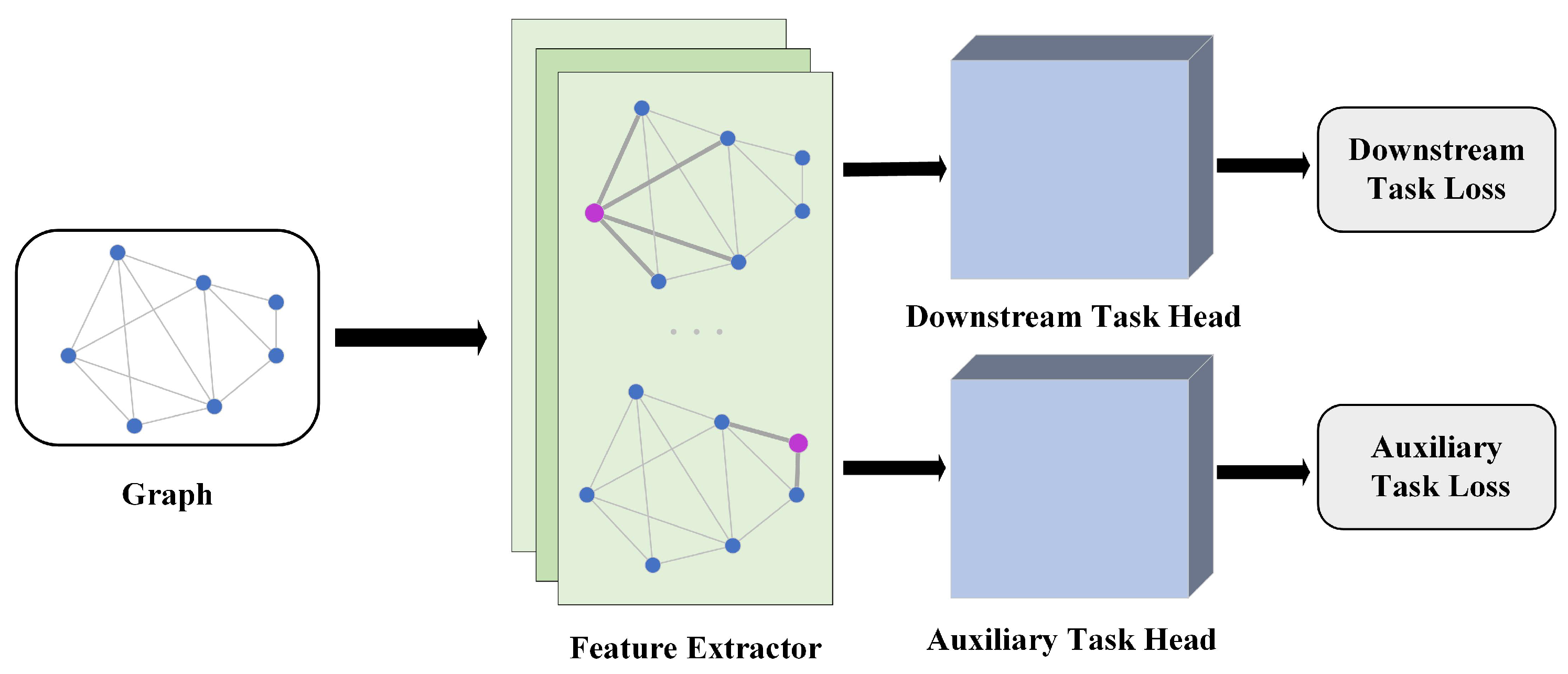
Inspired by joint learning, we developed GinfoNN, which can effectively exploit the properties of graph information. The goal of joint learning is to improve the generalization of the model by simultaneously minimizing the objective function of the downstream task and the auxiliary task. We briefly introduce the workflow of joint learning on GNNs, as shown in Figure 4. Joint learning can be divided into three parts: (1) a feature extractor; (2) a downstream task head and (3) an auxiliary task head. First, we need a feature extractor to transform node features into node representations, which can be arbitrary types and numbers of layers of GNNs. Based on the extracted node representations, the downstream task head transforms the features into prediction results and the auxiliary task head transforms the features into the corresponding output. Both the downstream task head and the auxiliary task head can be either a GNN or a linear transformation layer. Finally, we jointly optimize the objective functions of the downstream and auxiliary tasks.
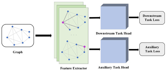
Figure 4.
An overview of the GinfoNN framework.
Feature Extractor. The Feature extractor is a layer of spatial GNNs that learns the weights of neighboring nodes and aggregates the node features of neighboring nodes according to the weights. According to the experimental results of AGNN on large and dense datasets, we want to utilize the node features as much as possible. Therefore, we choose the 2-layer MLP as the LTS to convert the concatenated node features into weights. The calculation formula is shown as
where means the concatenation operator. The forward propagation formula of the feature extractor is
where means the activation function, which is the ReLU function.
Downstream Task Head. The downstream task head is a layer of spatial GNNs, which transforms the latent node representations generated by the feature extractor into the target node representations for a specific task. To improve the computational efficiency, we do not calculate the weights of neighboring nodes in this layer, instead, use the weights obtained by the feature extractor directly. The forward propagation formula of the downstream task head is
Auxiliary Task Head. The auxiliary task head is a transformation function, which transforms the latent node representations generated by the feature extractor into the Ricci curvature. Then, we choose a two-layer MLP as the auxiliary task head. Note that the Ricci curvature is edge-specific. We need to use the cosine function to transform the outputs of those two nodes of an edge into a scalar. The forward propagation formula of the auxiliary task head is shown as
where cos indicates the cosine function.
Loss Function. The loss function of GinfoNN consists of the downstream task loss and the auxiliary task loss. Since the benchmark datasets are for node classification, we select the cross entropy as the downstream task loss. For the auxiliary task, we notice that the Ricci curvature is continuous and is distributed in . We select the mean squared error (MSE) as the auxiliary loss function. Besides, we also adjust the importance of task–auxiliary loss through the hyperparameter . The loss function of GinfoNN is
where is the one-hot encoding of node labels, and is the Ricci curvature of edge .
GinfoNN utilizes both label information and the Ricci Curvature to improve the generalization of GNNs. Unlike CurvGN which uses the Ricci Curvature as the input of LTS, GinfoNN uses it as the supervision signal of the auxiliary task head. GinfoNN effectively solves GIV and improves the performance of the model by exploiting the Ricci Curvature. In this way, we can easily and effectively take advantage of various graph information to enrich and improve the performance and knowledge of GNNs.
5. Experiments and Results
5.1. Databases
We select seven node classification benchmark datasets: Cora, Citeseer, PubMed, Coauthor CS, Coauthor Physics, Amazon Computers, and Amazon Photos. The detailed statistics of these seven datasets are shown in Table 5. For all datasets, the training set consists of 20 nodes per class, the validation set has 500 nodes, and the test set has 1000 nodes. Cora, Citeseer, and PubMed [39] have been widely used to evaluate the performance of GNNs, while these three benchmark datasets suffer from the disadvantages of a small total number of nodes and sparse connections. We added four more datasets, Coauthor CS, Coauthor Physics, Amazon Computers, and Amazon Photos, with a relatively larger number of nodes, number of edges, and average node degree. Coauthor CS and Coauthor Physics are used in the KDD Cup 2016 challenge and are based on the co-authorship graphs obtained from the Microsoft Academic Graph. The node features are word vectors extracted from the keywords of all papers of each author, and the classes represent the most active research areas of the authors. Amazon Computers and Amazon Photo are subgraphs of the Amazon co-purchase graph [40] with nodes representing items, edges representing two items often purchased at the same time, node features extracted from product reviews as word vectors, and classes representing product categories. We use pytorch_geometric [41] for the graph data loading and construction. In order to achieve better training for all models, we adopt feature normalization. All datasets are partitioned in the same way as in [42].
Table 5.
Statistic details of the benchmark datasets used in the experiments.
5.2. Experimental Setup
5.2.1. Baselines
To fairly evaluate the performance of GinfoNN, we chose some other important GNNs as baselines, in addition to the above five implicit GNNs: CurvGN, PEGN, GAT, HGCN, and AGNN. These baselines include spectral GNNs and spatial GNNs. GCN uses node degree to evaluate the importance of neighboring nodes. MoNet [22] not only proposes a unified framework for GNNs but also generalizes CNNs to non-Euclidean data, such as graphs and manifolds. GraphSAGE [10] proposed a neighboring sampling technique and three ways to aggregate neighboring node features and generalize GNNs from transductive learning to inductive learning. APPNP [11] introduces PageRank into GNNs and constructs a high-level node propagation mechanism. CGNN [43] explicitly transforms the Ricci curvature into weights in the aggregation process through the negative curvature transformation module and the curvature normalization module.
5.2.2. Set-Up
To enhance the reproducibility of the experiments, we choose 2021 as the random seed. We utilize the Adam stochastic gradient descent optimizer with a learning rate of 0.005 and L2 regularization of 0.0005 for training. We initialize the weight matrix with Glorot initialization. We use an early stopping strategy based on the validation set’s accuracies with a patience of 100 epochs. In this paper, for all statistic results (Table 2 and Table 6), we repeat 50 experiments (runs) for each model and use the average classification accuracy of the test set and its standard deviation as the main evaluation metric. For GinfoNN, we only adjust the hyperparameter , which represents the importance of the auxiliary task loss. We train all models on a single Nvidia 2080Ti, and the code for the models is built on pytorch_geometric [41].
Table 6.
Summary of statistical results in terms of mean test set classification accuracies (in percent) and standard deviation on seven node classification benchmark datasets. Red numbers mean the best accuracies, and bolded numbers mean the second-best performance. OOM means out of memory.
5.3. Curvature Boosts Generalization
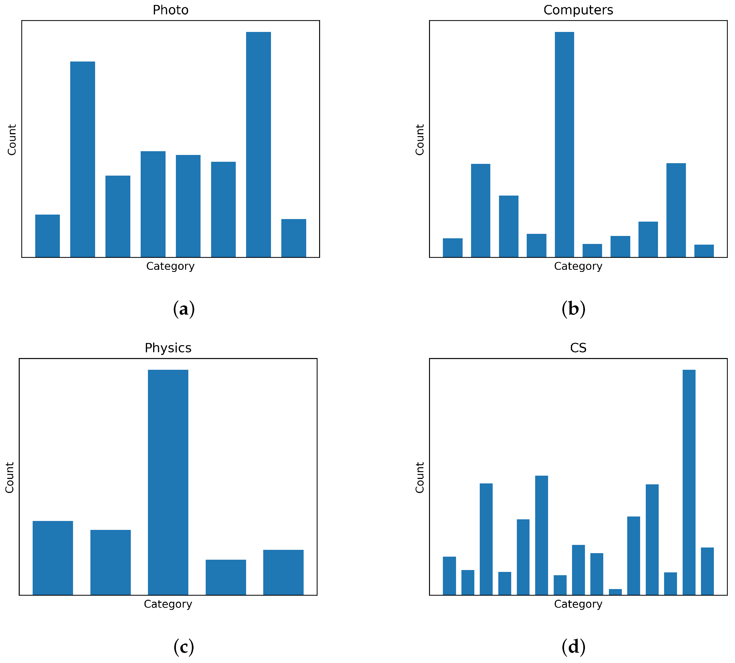
The mechanism of GinfoNN and the structural property of the Ricci curvature improve the generalization of GNNs together. The classification accuracies and F1-score of GinfoNN and the baselines on the seven node classification benchmark datasets are shown in Table 6 and Table 7, respectively. Experimental results evaluated by both accuracy and weighted F1-score indicate that GinfoNN outperforms the baselines on large and dense datasets. The reason is that Ricci curvature effectively describes the interactions between neighboring nodes within the local topological structure, serving as a kind of unique and valuable graph information. Preserving this information promotes the model to distinguish the categorical properties of nodes and edges. Explicitly leveraging the learning of Ricci curvature as an auxiliary task not only prevents the vanishing of graph information represented by Ricci curvature but also acts as a supervision signal as a constraint of learning node representations. Therefore, GinfoNN provides GNNs with the Ricci curvature as an auxiliary but valuable supervision signal, effectively compensating for the shortcomings. It enables GinfoNN to perform the best classification on large and dense datasets. As shown in Figure 5, it can be observed that the four added datasets exhibit a significant imbalance of categorical distribution, which affects the propagation of label information across the whole graph. Due to the small proportion of labeled nodes (20 nodes per class), the supervision signal provided by labels on large-scale datasets is insufficient to transmit to the full graph. This imbalance of global spatial distribution makes it even more challenging for the signal to transmit effectively.
Table 7.
Summary of statistical results in terms of mean test set classification F1-score (in percent) and standard deviation on seven node classification benchmark datasets. We adopted the weighted form of the F1-score. Red numbers mean the best accuracies, and bolded numbers mean the second-best performance. OOM means out of memory.

Figure 5.
The categorical distribution of four added datasets. The horizontal axis represents different node categories, and the vertical axis indicates the number of nodes in each category: (a) Photos; (b) Computers; (c) Physics; (d) CS.
Meanwhile, we find that the performance of APPNP is optimal on small datasets. This is because APPNP improves the propagation mechanism of node features based on PageRank, which gives the target node a larger perceptive field. However, GinfoNN still achieves comparable classification accuracies compared with the baselines. This indicates that the Ricci curvature as an auxiliary supervision signal does not interfere with the supervision signal provided by the label and impairs the performance of GNNs. The experimental results illustrate that auxiliary supervision signals are crucial for improving the performance of GNNs when the dataset is large, dense, and relatively underlabeled.
5.4. Ablation Experiment
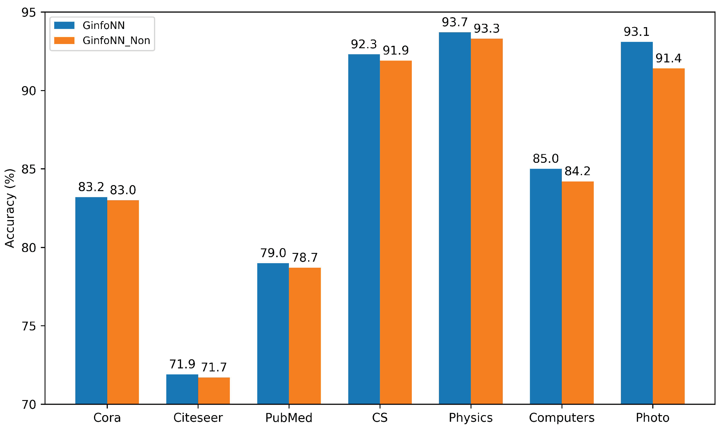
In this subsection, we design the ablation experiment to illustrate the necessity of the auxiliary task head. If the auxiliary task head is removed, it would impair the generalization of GinfoNN. Figure 6 shows the classification accuracies of GinfoNN with the auxiliary task head and GinfoNN with the auxiliary task head removed on the seven benchmark datasets. We find that the classification accuracies of GinfoNN and GinfoNN_Non are close on relatively small and sparse datasets. Nevertheless, the classification accuracies of GinfoNN are significantly better than GinfoNN_Non on the large and dense datasets. In particular, on the Photo dataset, GinfoNN improves by 1.5 percentage points. This ablation experiment illustrates that the auxiliary task head effectively improves the generalizability of GNNs.
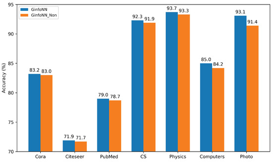
Figure 6.
Comparison of predicted accuracies of GinfoNN with and without the auxiliary task head. GinfoNN_Non means GinfoNN without the auxiliary task head.
6. Discussion
Applications on real-world task scenarios. A graph is a crucial data type widely present in various fields. Graph representation learning also holds significant practical value, such as user classification in social networks, risk assessment in financial systems, recommendation systems, etc. GinfoNN is a general graph representation learner, making it applicable to various tasks across different domains. Additionally, Ricci curvature represents different physical meanings in different fields. For example, in transportation networks, Ricci curvature can be used to identify bottleneck segments [44]. Therefore, understanding graph data and graph information in real-world applications enables better adaptation of GinfoNN to practical applications while providing interpretable insights.
Extentions to more learning paradigms and other types of graph information. Explicitly incorporating the learning of Ricci curvature as a constraint during the model’s representation learning process can help prevent the model from falling into the GIV dilemma. In this paper, Ricci curvature is selected as a form of effective graph information, and joint learning is chosen as the learning method, providing a preferable way for addressing the GIV issue. In the future, new learning paradigms such as self-supervised learning [45,46] and zero-shot learning, as well as the introduction of other types of graph information, can be further explored.
Generalizations on heterophilic graphs. The selected datasets are all high-homophily, which is also the main type in graph benchmark datasets. However, there exists a type of high-heterophily dataset [47], where the interactions between neighboring nodes show entirely different meanings. Whether Ricci curvature in heterophilic datasets will exhibit different properties, and whether it can provide equally effective information are questions that can be explored in the future.
7. Conclusions
In this paper, we find the existence of GIV for implicit GNNs, which leads to that GNNs do not exploit the property of graph information. We first show that random value substitution does not significantly affect the performance of implicit GNNs through extensive experiments. Then, we find that the weights of neighbors generated by the LTS using different graph information have high similarity from both qualitative and quantitative perspectives. Empirical experiments suggest that GIV does exist for implicit GNNs. Inspired by joint learning, we propose GinfoNN, which uses the Ricci curvature as an auxiliary supervision signal to constrain the training of the feature extractor. The experimental results show that GinfoNN outperforms baselines on heterogeneously large and dense datasets. GinfoNN provides new insights into how GNNs can utilize various valuable graph information.
Author Contributions
Conceptualization, J.C. and S.H.; methodology, J.C. and S.H.; software, H.Y. and Z.C.; validation, H.Y. and Z.C.; formal analysis, S.H.; investigation, H.Y. and Z.C.; resources, H.L.; data curation, H.Y.; writing—original draft preparation, J.C. and S.H.; writing—review and editing, J.C. and S.H.; visualization, J.C.; supervision, H.L.; project administration, S.G.; funding acquisition, S.G. All authors have read and agreed to the published version of the manuscript.
Funding
This research was funded by the National Natural Science Foundation of China, Grant Numbers: 62207032; Research Foundation of the Department of Natural Resources of Hunan Province, Grant Numbers: HBZ20240101; Scientific Research Project of the Department of Education of Hunan Province, Grant Numbers: 22B0014.
Institutional Review Board Statement
Not applicable.
Informed Consent Statement
Not applicable.
Data Availability Statement
No new data were created or analyzed in this study. Data sharing is not applicable to this article.
Acknowledgments
We acknowledge the High-Performance Computing Platform of Central South University and HPC Central of the Department of GIS for providing HPC resources.
Conflicts of Interest
The authors declare no conflicts of interest.
Abbreviations
The following abbreviations are used in this manuscript:
| GNN | Graph Neural Network |
| LTS | Learnable Transformation Structure |
| GIV | Graph Information Vanishing |
References
- Zhang, M.; Chen, Y. Link prediction based on graph neural networks. In Proceedings of the 32nd International Conference on Neural Information Processing Systems, Red Hook, NY, USA, 3–8 December 2018; pp. 5171–5181. [Google Scholar]
- Bian, T.; Xiao, X.; Xu, T.; Zhao, P.; Huang, W.; Rong, Y.; Huang, J. Rumor detection on social media with bi-directional graph convolutional networks. In Proceedings of the AAAI Conference on Artificial Intelligence, New York, NY, USA, 7–12 February 2020; Volume 34, pp. 549–556. [Google Scholar]
- Yu, B.; Yin, H.; Zhu, Z. Spatio-temporal graph convolutional networks: A deep learning framework for traffic forecasting. In Proceedings of the 27th International Joint Conference on Artificial Intelligence, Stockholm, Sweden, 13–19 July 2018; pp. 3634–3640. [Google Scholar]
- Kosaraju, V.; Sadeghian, A.; Martín-Martín, R.; Reid, I.D.; Rezatofighi, H.; Savarese, S. Social-BiGAT: Multimodal trajectory forecasting using Bicycle-GAN and graph attention networks. In Proceedings of the Advances in Neural Information Processing Systems, Neural Information Processing Systems (NIPS), Vancouver, BC, Canada, 8–14 December 2019. [Google Scholar]
- Duvenaud, D.; Maclaurin, D.; Aguilera-Iparraguirre, J.; Gómez-Bombarelli, R.; Hirzel, T.; Aspuru-Guzik, A.; Adams, R.P. Convolutional networks on graphs for learning molecular fingerprints. In Proceedings of the 28th International Conference on Neural Information Processing Systems, Cambridge, MA, USA, 7–12 December 2015; Volume 2, pp. 2224–2232. [Google Scholar]
- Jin, W.; Yang, K.; Barzilay, R.; Jaakkola, T. Learning Multimodal Graph-to-Graph Translation for Molecule Optimization. In Proceedings of the International Conference on Learning Representations, Vancouver, BC, Canada, 30 April–3 May 2018. [Google Scholar]
- Gilmer, J.; Schoenholz, S.S.; Riley, P.F.; Vinyals, O.; Dahl, G.E. Neural message passing for quantum chemistry. In Proceedings of the International Conference on Machine Learning, Sydney, NSW, Australia, 6–11 August 2017; pp. 1263–1272. [Google Scholar]
- Kipf, T.N.; Welling, M. Semi-supervised classification with graph convolutional networks. arXiv 2016, arXiv:1609.02907. [Google Scholar]
- Veličković, P.; Cucurull, G.; Casanova, A.; Romero, A.; Lio, P.; Bengio, Y. Graph attention networks. arXiv 2017, arXiv:1710.10903. [Google Scholar]
- Hamilton, W.L.; Ying, R.; Leskovec, J. Inductive representation learning on large graphs. In Proceedings of the 31st International Conference on Neural Information Processing Systems, Red Hook, NY, USA, 4–9 December 2017; pp. 1025–1035. [Google Scholar]
- Klicpera, J.; Bojchevski, A.; Günnemann, S. Predict then propagate: Graph neural networks meet personalized pagerank. arXiv 2018, arXiv:1810.05997. [Google Scholar]
- Zhang, K.; Zhu, Y.; Wang, J.; Zhang, J. Adaptive structural fingerprints for graph attention networks. In Proceedings of the International Conference on Learning Representations, New Orleans, LA, USA, 6–9 May 2019. [Google Scholar]
- Xu, K.; Hu, W.; Leskovec, J.; Jegelka, S. How powerful are graph neural networks? arXiv 2018, arXiv:1810.00826. [Google Scholar]
- Ye, Z.; Liu, K.S.; Ma, T.; Gao, J.; Chen, C. Curvature graph network. In Proceedings of the International Conference on Learning Representations, New Orleans, LA, USA, 6–9 May 2019. [Google Scholar]
- Lin, Y.; Lu, L.; Yau, S.T. Ricci curvature of graphs. Tohoku Math. J. Second Ser. 2011, 63, 605–627. [Google Scholar] [CrossRef]
- Zhao, Q.; Ye, Z.; Chen, C.; Wang, Y. Persistence enhanced graph neural network. In Proceedings of the International Conference on Artificial Intelligence and Statistics, Online, 26–28 August 2020; pp. 2896–2906. [Google Scholar]
- Chami, I.; Ying, R.; Ré, C.; Leskovec, J. Hyperbolic graph convolutional neural networks. Adv. Neural Inf. Process. Syst. 2019, 32, 4869. [Google Scholar]
- Thekumparampil, K.K.; Wang, C.; Oh, S.; Li, L.J. Attention-based graph neural network for semi-supervised learning. arXiv 2018, arXiv:1803.03735. [Google Scholar]
- Ollivier, Y. Ricci curvature of metric spaces. C. R. Math. 2007, 345, 643–646. [Google Scholar] [CrossRef]
- Bruna, J.; Zaremba, W.; Szlam, A.; LeCun, Y. Spectral networks and locally connected networks on graphs. arXiv 2013, arXiv:1312.6203. [Google Scholar]
- Defferrard, M.; Bresson, X.; Vandergheynst, P. Convolutional neural networks on graphs with fast localized spectral filtering. In Proceedings of the 30th International Conference on Neural Information Processing Systems, Barcelona, Spain, 5–10 December 2016; pp. 3844–3852. [Google Scholar]
- Monti, F.; Boscaini, D.; Masci, J.; Rodola, E.; Svoboda, J.; Bronstein, M.M. Geometric deep learning on graphs and manifolds using mixture model cnns. In Proceedings of the IEEE Conference on Computer Vision and Pattern Recognition, Honolulu, HI, USA, 21–26 July 2017; pp. 5115–5124. [Google Scholar]
- Li, Y.; Wang, X.; Liu, H.; Shi, C. A generalized neural diffusion framework on graphs. In Proceedings of the AAAI Conference on Artificial Intelligence, Vancouver, BC, Canada, 20–27 February 2024; Volume 38, pp. 8707–8715. [Google Scholar]
- Li, Q.; Han, Z.; Wu, X.M. Deeper insights into graph convolutional networks for semi-supervised learning. In Proceedings of the AAAI Conference on Artificial Intelligence, New Orleans, LA, USA, 2–7 February 2018; Volume 32. [Google Scholar]
- Oono, K.; Suzuki, T. Graph Neural Networks Exponentially Lose Expressive Power for Node Classification. In Proceedings of the International Conference on Learning Representations, New Orleans, LA, USA, 6–9 May 2019. [Google Scholar]
- Barceló, P.; Kostylev, E.; Monet, M.; Pérez, J.; Reutter, J.; Silva, J.P. The logical expressiveness of graph neural networks. In Proceedings of the 8th International Conference on Learning Representations (ICLR 2020), Addis Ababa, Ethiopia, 26–30 April 2020. [Google Scholar]
- Agarwal, C.; Zitnik, M.; Lakkaraju, H. Probing gnn explainers: A rigorous theoretical and empirical analysis of gnn explanation methods. In Proceedings of the International Conference on Artificial Intelligence and Statistics, Virtual, 28–30 March 2022; pp. 8969–8996. [Google Scholar]
- Wu, F.; Souza, A.; Zhang, T.; Fifty, C.; Yu, T.; Weinberger, K. Simplifying graph convolutional networks. In Proceedings of the International Conference on Machine Learning, Long Beach, CA, USA, 9–15 June 2019; pp. 6861–6871. [Google Scholar]
- Li, G.; Muller, M.; Thabet, A.; Ghanem, B. Deepgcns: Can gcns go as deep as cnns? In Proceedings of the IEEE/CVF International Conference on Computer Vision, Seoul, Republic of Korea, 27 October–2 November 2019; pp. 9267–9276. [Google Scholar]
- Knyazev, B.; Taylor, G.W.; Amer, M. Understanding Attention and Generalization in Graph Neural Networks. Adv. Neural Inf. Process. Syst. 2019, 32, 4202–4212. [Google Scholar]
- You, Y.; Chen, T.; Wang, Z.; Shen, Y. When does self-supervision help graph convolutional networks? In Proceedings of the International Conference on Machine Learning, Online, 26–28 August 2020; pp. 10871–10880. [Google Scholar]
- Sun, K.; Lin, Z.; Zhu, Z. Multi-stage self-supervised learning for graph convolutional networks on graphs with few labeled nodes. In Proceedings of the AAAI Conference on Artificial Intelligence, New York, NY, USA, 7–12 February 2020; Volume 34, pp. 5892–5899. [Google Scholar]
- Jin, W.; Derr, T.; Liu, H.; Wang, Y.; Wang, S.; Liu, Z.; Tang, J. Self-supervised learning on graphs: Deep insights and new direction. arXiv 2020, arXiv:2006.10141. [Google Scholar]
- Hu, Z.; Fan, C.; Chen, T.; Chang, K.W.; Sun, Y. Pre-training graph neural networks for generic structural feature extraction. arXiv 2019, arXiv:1905.13728. [Google Scholar]
- Ding, Q.; Ye, D.; Xu, T.; Zhao, P. GPN: A Joint Structural Learning Framework for Graph Neural Networks. arXiv 2022, arXiv:2205.05964. [Google Scholar]
- Gui, S.; Liu, M.; Li, X.; Luo, Y.; Ji, S. Joint Learning of Label and Environment Causal Independence for Graph Out-of-Distribution Generalization. In Proceedings of the Thirty-Seventh Conference on Neural Information Processing Systems, New Orleans, LA, USA, 10–16 December 2023. [Google Scholar]
- Ni, C.C.; Lin, Y.Y.; Gao, J.; Gu, X.D.; Saucan, E. Ricci curvature of the internet topology. In Proceedings of the 2015 IEEE Conference on Computer Communications (INFOCOM), Kowloon, Hong Kong, 26 April–1 May 2015; pp. 2758–2766. [Google Scholar]
- Sia, J.; Jonckheere, E.; Bogdan, P. Ollivier-ricci curvature-based method to community detection in complex networks. Sci. Rep. 2019, 9, 9800. [Google Scholar] [CrossRef] [PubMed]
- Sen, P.; Namata, G.; Bilgic, M.; Getoor, L.; Galligher, B.; Eliassi-Rad, T. Collective classification in network data. AI Mag. 2008, 29, 93. [Google Scholar] [CrossRef]
- McAuley, J.; Targett, C.; Shi, Q.; Van Den Hengel, A. Image-based recommendations on styles and substitutes. In Proceedings of the 38th International ACM SIGIR Conference on Research and Development in Information Retrieval, Santiago, Chile, 9–13 August 2015; pp. 43–52. [Google Scholar]
- Fey, M.; Lenssen, J.E. Fast graph representation learning with PyTorch Geometric. arXiv 2019, arXiv:1903.02428. [Google Scholar]
- Shchur, O.; Mumme, M.; Bojchevski, A.; Günnemann, S. Pitfalls of graph neural network evaluation. arXiv 2018, arXiv:1811.05868. [Google Scholar]
- Li, H.; Cao, J.; Zhu, J.; Liu, Y.; Zhu, Q.; Wu, G. Curvature Graph Neural Network. arXiv 2021, arXiv:2106.15762. [Google Scholar] [CrossRef]
- Han, X.; Zhu, G.; Zhao, L.; Du, R.; Wang, Y.; Chen, Z.; Liu, Y.; He, S. Ollivier–Ricci Curvature Based Spatio-Temporal Graph Neural Networks for Traffic Flow Forecasting. Symmetry 2023, 15, 995. [Google Scholar] [CrossRef]
- Li, H.; Cao, J.; Zhu, J.; Luo, Q.; He, S.; Wang, X. Augmentation-free graph contrastive learning of invariant-discriminative representations. IEEE Trans. Neural Netw. Learn. Syst. 2024, 35, 11157–11167. [Google Scholar] [CrossRef]
- Zhang, Z.; Ren, Z.; Tao, C.; Zhang, Y.; Peng, C.; Li, H. Grass: Contrastive learning with gradient guided sampling strategy for remote sensing image semantic segmentation. IEEE Trans. Geosci. Remote. Sens. 2023, 61, 5626814. [Google Scholar] [CrossRef]
- He, S.; Luo, Q.; Fu, X.; Zhao, L.; Du, R.; Li, H. Cat: A causal graph attention network for trimming heterophilic graphs. Inf. Sci. 2024, 677, 120916. [Google Scholar] [CrossRef]

Disclaimer/Publisher’s Note: The statements, opinions and data contained in all publications are solely those of the individual author(s) and contributor(s) and not of MDPI and/or the editor(s). MDPI and/or the editor(s) disclaim responsibility for any injury to people or property resulting from any ideas, methods, instructions or products referred to in the content. |
© 2024 by the authors. Licensee MDPI, Basel, Switzerland. This article is an open access article distributed under the terms and conditions of the Creative Commons Attribution (CC BY) license (https://creativecommons.org/licenses/by/4.0/).