Explicit Analysis for the Ground Reaction of a Circular Tunnel Excavated in Anisotropic Stress Fields Based on Hoek–Brown Failure Criterion

Abstract

The study aims to utilize the convergence–confinement method (CCM) by considering non-hydrostatic stress assumptions in the analysis of the surrounding rock in a circular tunnel. The rock mass properties should adhere to the criteria of the non-linear Hoek–Brown failure criterion. Through a thorough theoretical analysis approach, an analytical solution was derived to determine the stress and displacement induced by tunnel excavation, particularly in the elastic and plastic zones. This solution, applicable under anisotropic stress conditions, involves accounting for confinement loss incrementally for computational feasibility. The implementation of this analytical solution, facilitated by a straightforward spreadsheet, was validated against existing data to evaluate the impact of non-linear failure criteria on ground reaction behavior. The study scrutinizes the mechanical response at the tunnel’s inner curve and assesses stress–displacement distribution across the tunnel cross-section. A comparison between the proposed solution and published results demonstrates a consistent and promising correlation.

1. Introduction

The convergence–confinement method (CCM) is a systematic strategy employed for tunnel design and construction in rock formations. It acknowledges the natural tendency of rock masses to deform and converge around excavated tunnels as stress redistributes. The primary goal of this method is to regulate and address such convergence by offering sufficient confinement or support to guarantee the stability and safety of the tunnel [1,2].

This method offers a structure for comprehending and controlling the convergence characteristics of the rock masses. The design of support then translates this comprehension into tangible actions aimed at improving tunnel stability [3,4]. The core principle of the CCM revolves around how the primary and secondary stress fields interact during tunnel excavation. As the tunnel is dug out, the primary stress within the rock masses undergoes redistribution, prompting the rock to deform and converge towards the opening. This convergence may trigger displacements, deformations, and potentially unstable situations if not effectively managed [5,6,7,8,9].

The CCM focuses on achieving three main objectives: (1) The ground reaction curve (GRC as shown by the ABCEG curve in Figure 1) aims to limit the amount of convergence and control the rate at which it occurs. By controlling convergence, the risk of tunnel deformation and failure is reduced. The level of acceptable convergence depends on factors such as the tunnel purpose, ground conditions, support system, and safety requirements [10,11,12,13,14,15]. (2) The support confining curve (SCC as shown by the DEI curve in Figure 1) involves applying external support to tunnel walls to counter inward movement and sustain stability. This is accomplished by implementing diverse support systems like rock bolts, shotcrete, steel ribs, or other reinforcement elements. These support elements aid in confining the rock masses and dispersing stresses, thereby minimizing convergence and fortifying tunnel stability [9,16,17,18,19,20,21]. (3) The confinement loss curve (CLC) underscores the significance of adopting an observational approach throughout tunnel construction. This entails constantly monitoring the rock mass’s behavior and adapting support measures accordingly. Confinement loss is determined by the correlation between convergence measurements and the unsupported distance to the tunnel face. It can take the form of a positive scalar, an incremental value, or a function to account for the impact of the advancing excavation of the tunnel face [22,23,24,25,26]. Through the adoption of the convergence-confinement method, engineers can efficiently regulate the convergence tendencies of rock masses in tunneling endeavors. This method offers a structured and preemptive strategy, guaranteeing the stability and safety of subterranean excavations [15,27].

In the convergence–confinement method, the ground reaction curve (GRC) serves as a fundamental concept for comprehending how the rock masses and support system react to tunnel excavation. It delineates the correlation between tunnel wall convergence (displacement) and the applied support pressure. Moreover, the failure criterion offers a valuable understanding of the strength and behavior of the rock masses, shaping the features of the ground reaction curve. This study explores and applies the characteristics of the GRC using the nonlinear failure criterion of generalized Hoek–Brown [28,29,30]. This criterion enables engineers to evaluate the stability of rock slopes or tunnels across varying stress conditions, factoring in the strength and integrity of the rock masses. It serves as a tool for assessing the stability of the rock masses and determining the necessary support measures during tunneling operations [31,32,33,34]. Employing the generalized Hoek–Brown failure criterion enables engineers to gauge the strength of the rock masses and anticipate potential failure mechanisms during tunneling activities. This insight is vital for selecting suitable support systems and establishing the necessary support pressure to manage convergence and uphold tunnel stability [35,36,37,38].

The convergence–confinement method (CCM) is widely used in conventional tunneling at a preliminary stage of the support design. A circular tunnel through the ground in an initially isotropic stress state and the behavior of ground–support interaction, simplified utilizing a two-dimensional plane-strain, were postulated in the references [5,39]. Reference [5] described that the direct algorithm process was proposed in their paper to deal with solving the solution of stresses/displacements between the ground reaction curve (GRC) and the support confining curve (SCC) in the final equilibrium state by applying the simultaneous equations in the elastic region and using the numerical analysis known as the Newton recursion method for finding roots of the non-linear equations in the plastic region. In addition, reference [39] introduced the Hoek–Brown nonlinear failure criterion into the ground reaction curve (GRC) of the convergence–confinement method (CCM) in tunneling under isotropic stress conditions.

Finally, the generalized Hoek–Brown failure criterion serves as a foundation for comprehending the strength and failure characteristics of the rock masses. Meanwhile, the ground reaction curve offers a method to assess the real-time response of the rock masses and support systems during tunneling endeavors. The failure criterion guides the design of the support system, while the ground reaction curve verifies its efficacy. Together, these principles play a pivotal role in the comprehensive evaluation and control of convergence and confinement within the convergence–confinement method for tunneling projects.

General tunnel excavation and support design methods can be summarized into the following four types: (1) define the rock mass classification system based on pure empirical rules and summarize the most appropriate tunnel excavation support system; (2) regardless of support type and deformation, determine the support system based on tunnel stress load; (3) according to the geological conditions of the tunnel, the stiffness and deformation of the support system are considered, and the load of the tunnel support system is designed; and (4) the analysis method of the interaction between the tunnel excavation surrounding rock and the structural support system [1,2,3,4]. These numerical analysis methods include the finite element method, finite difference method, boundary element method, distinct element method, discontinuous deformation analysis, etc., to simulate the interaction between the surrounding rock and the structural support system in tunneling. However, establishing and using numerical analysis methods still requires theoretical analysis and formula derivation as the basic basis. Therefore, this study focuses on the convergence of the surrounding rock during tunnel excavation and explores the changes in the elastic-plastic mechanical behavior of the surrounding rock caused by tunnel excavation under anisotropic stress field conditions.

Excavating tunnels in rock masses often involves dealing with complex stress distributions. Traditional analysis methods may not adequately account for the effects of anisotropic stress fields, which are common in geological formations. This research aims to address this gap by applying the Hoek–Brown failure criterion to analyze the ground reaction of circular tunnels under these conditions. Therefore, this paper aims to offer a thorough examination of the non-linear failure criterion of generalized Hoek–Brown concerning ground reaction within the convergence–confinement method for tunnel support design. This includes presenting the complete set of equations along with the details of their derivation, verification, and comparison. Additionally, illustrative diagrams depicting stress/displacement distributions at the intrados and across tunnel cross-sections will be provided.

2. Problem Description

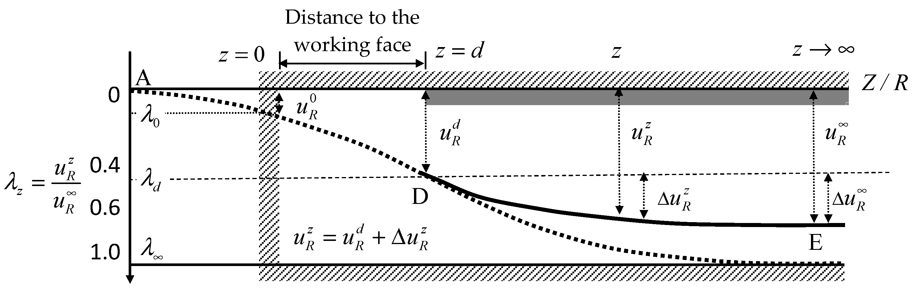
2.1. Correlation between Confinement Loss and the Advancing Excavation of Tunnels

The progressive excavation of the tunnel face induces a shift in the stress field within the surrounding rock, leading to stress redistribution and convergence of the excavation face. Put simply, the impact of advancing tunnel excavation involves monitoring stress and displacement changes caused by sequential excavation at specific measurement points along an observation section. This study primarily suggests employing tunnel convergence measurements, developing functions to address the effects of advancing tunnel excavation, and outlining procedures for estimating confinement loss.

Furthermore, the role of the confinement loss curve (CLC) can be depicted in Figure 2, where at a specific distance (z) from the working face, the definition of confinement loss (λ_z) can be provided as [5,6]:

$${\lambda }_z={\lambda }_0+\left(1-{\lambda }_0\right)\left[1-{\left({\displaystyle \frac{m}{m+\frac{z}{R}}}\right)}^2\right]$$

(1)

where R represents the tunnel excavation radius, and λ₀ denotes the confinement loss at the working face (z = 0, point A in Figure 1) and can be expressed as:

$${\lambda }_0=1-{\left({\displaystyle \frac{m}{m+\frac{d}{R}}}\right)}^2$$

(2)

2.2. Variations in Stress around a Circular Tunnel

The convergence–confinement method revolves around analyzing the stress and strain states that arise in the rock masses surrounding a tunnel. Excavating the tunnel alters stresses at its periphery. Therefore, stress variations are primarily understood through the stress gradient, which denotes the difference between far-field and near-field stresses around the tunnel. In numerical analysis, stress increments consider the confinement loss (λ) as a portion of the stress gradient, a crucial principle in the convergence-confinement method. Stress variations are described by the following formulations [5,6]:

(1)

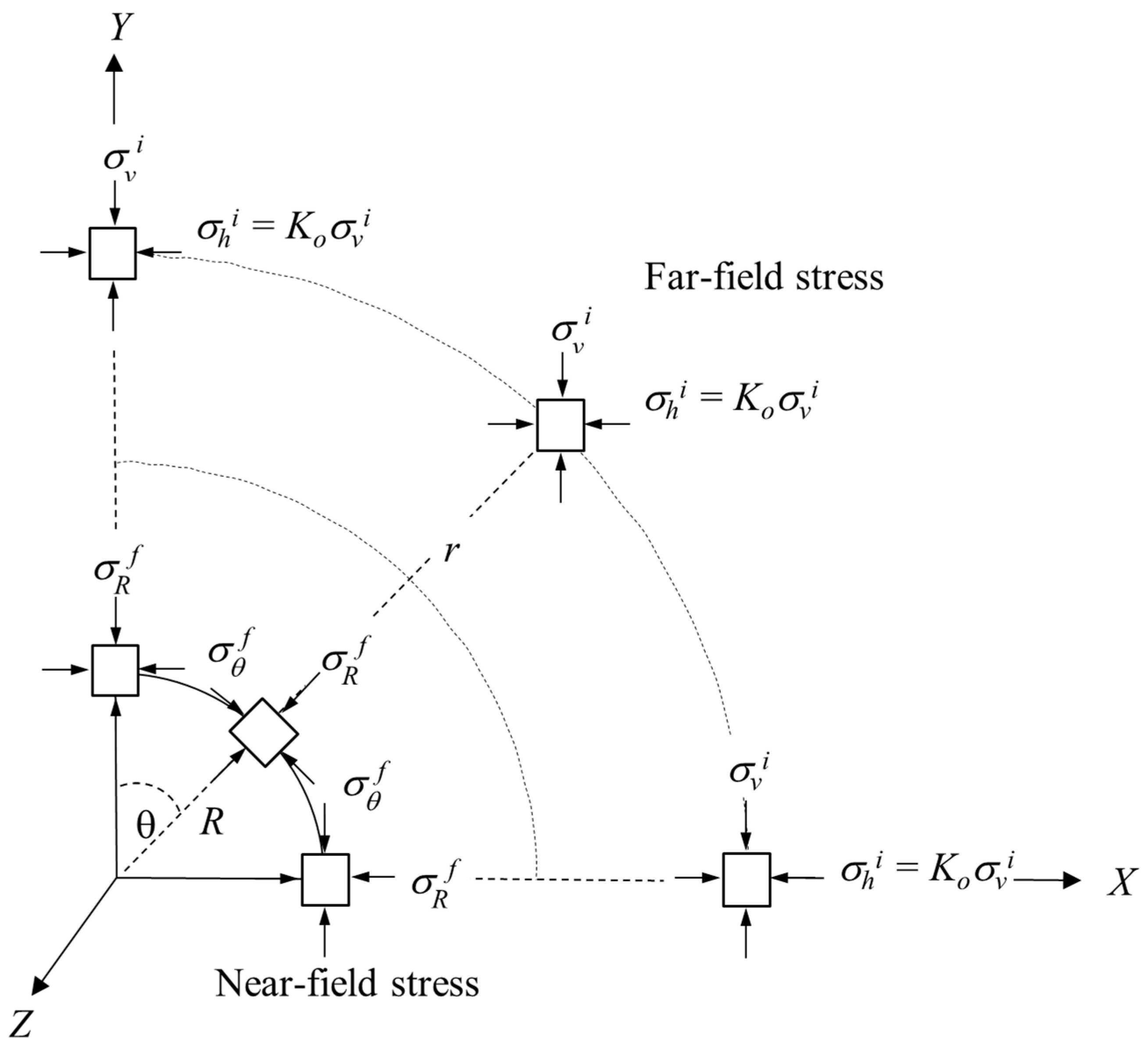
Stresses in the far field (initial in situ stresses, as r → ∞): Before tunnel excavation, the stresses within the rock masses are in equilibrium and mirror the lithostatic stresses, remaining constant in the surrounding medium of the tunnel. Thus, the initial anisotropic stress within the rock masses can be illustrated as depicted in Figure 3 and represented by the following equation:

$${\sigma }_r^i={\displaystyle \frac{{\sigma }_v}{2}}\left(k_1+k_2\right)$$

(3)

$${\sigma }_{\theta }^i={\displaystyle \frac{{\sigma }_v}{2}}\left(k_1-k_2\right)$$

(4)

where ${\sigma }_r^i$, ${\sigma }_{\theta }^i$, and ${\sigma }_v$ are the initial radial stress, the initial tangential stress, and the vertical stress in the polar coordinates (r, θ), respectively. Moreover, the coefficients k₁ = 1 + K₀, k₂ = (1 − K_o)cosθ, and K_o is the lateral stress ratio (K_o = σ_h/σ_v = horizontal stress/vertical stress).

(2)

Stresses in the near field (final stresses or boundary stresses at the tunnel periphery, R ≤ r < ∞): Upon tunnel excavation, the stresses at any given point within the rock masses surrounding the tunnel undergo alteration. These altered stresses can be determined using the Kirsch solutions, outlined as follows:

$${\sigma }_r^f={\displaystyle \frac{{\sigma }_v}{2}}\left[k_1\left(1-{\displaystyle \frac{R^2}{r^2}}\right)+k_2\left(1-4{\displaystyle \frac{R^2}{r^2}}+3{\displaystyle \frac{R^4}{r^4}}\right)\right]$$

(5)

$${\sigma }_{\theta }^f={\displaystyle \frac{{\sigma }_v}{2}}\left[k_1\left(1+{\displaystyle \frac{R^2}{r^2}}\right)-k_2\left(1+3{\displaystyle \frac{R^4}{r^4}}\right)\right]$$

(6)

where ${\sigma }_r^f$ and ${\sigma }_{\theta }^f$ are the final radial stress and the final tangential stress around the tunnel proximity, respectively.

If we presume that the stress gradient resulting from the progressive excavation of the tunnel face is the disparity between the far-field stress and the near-field stress, we can express the difference between the radial stress and the tangential stress using the following equations:

$${\overline{\sigma }}_r={\sigma }_r^f-{\sigma }_r^i$$

(7)

$${\overline{\sigma }}_{\theta }={\sigma }_{\theta }^f-{\sigma }_{\theta }^i$$

(8)

Employing the hypothesis of increments in numerical analysis, stress increments can be represented as the product of the stress gradient and the confinement loss λ, which is a fraction of the stress gradient. It can be calculated as follows:

$$∆{\sigma }_r=\lambda {\overline{\sigma }}_r=-{\displaystyle \frac{\lambda {\sigma }_v}{2}}\left[k_1\left({\displaystyle \frac{R^2}{r^2}}\right)+k_2\left(4{\displaystyle \frac{R^2}{r^2}}-3{\displaystyle \frac{R^4}{r^4}}\right)\right]$$

(9)

$$∆{\sigma }_{\theta }=\lambda {\overline{\sigma }}_{\theta }=+{\displaystyle \frac{\lambda {\sigma }_v}{2}}\left[k_1\left({\displaystyle \frac{R^2}{r^2}}\right)-3k_2\left({\displaystyle \frac{R^4}{r^4}}\right)\right]$$

(10)

Finally, the stress variation resulting from the advancing excavation of the tunnel (0 ≤ λ ≤ 1) at a specific point near the tunnel (r, θ) can be depicted as follows:

$${\sigma }_r={\sigma }_r^i+∆{\sigma }_r={\displaystyle \frac{{\sigma }_v}{2}}\left[k_1\left(1-\lambda {\displaystyle \frac{R^2}{r^2}}\right)+k_2\left(1-\lambda \left(4{\displaystyle \frac{R^2}{r^2}}-3{\displaystyle \frac{R^4}{r^4}}\right)\right)\right]$$

(11)

$${\sigma }_{\theta }={\sigma }_{\theta }^i+∆{\sigma }_{\theta }={\displaystyle \frac{{\sigma }_v}{2}}\left[k_1\left(1+\lambda {\displaystyle \frac{R^2}{r^2}}\right)-k_2\left(1+3\lambda {\displaystyle \frac{R^4}{r^4}}\right)\right]$$

(12)

Furthermore, based on the results derived from the Kirsch solution [40], the radial displacement (u_r) within the elastic region can be expressed as follows:

$${\displaystyle \frac{2G}{{\sigma }_v}}{\displaystyle \frac{u_r}{R}}={\displaystyle \frac{\mathsf{\lambda }}{2}}\left({\displaystyle \frac{R}{r}}\right)\left[k_1+k_2\left(4\left(1-\nu \right)-{\displaystyle \frac{R^2}{r^2}}\right)\right]$$

(13)

where G is the shear modulus of the rock masses.

It is necessary to note that these equations must conform to the boundary conditions stipulated by the convergence-confinement method. They can also be validated through the following interpretations: (1) when λ = 0, that the tunnel has not been excavated yet, and the stresses in the rock masses match the initial in situ stresses ${\sigma }_r^i$ and ${\sigma }_{\theta }^i$ (or the far-field stress, e.g., r → ∞), and (2) when λ = 1, indicating that the tunnel has been fully excavated, the stresses in the rock masses align with Kirsch’s stresses ${\sigma }_r^f$ and ${\sigma }_{\theta }^f$ (or the near-field stress, e.g., r = R).

3. Derivation of Stress/Displacement Equations in the Plastic Region

3.1. Derivation of the Confinement Loss in Elastic Limit with the Non-Linear Failure Criteria

In the broader context of rock masses exhibiting elastic/perfectly plastic behavior, the confinement loss in the elastic limit situation (λ_e) emerges as the elastic limit of the rock masses is attained, typically at a certain radial stress (σ_r) and with a decrease in radius (r), coinciding with the stress state reaching limit conditions defined by the strength criterion. This particular radius (R_p), termed the plastic radius, is not merely dependent on the peak strength parameters of the rock masses but is also influenced by the confinement loss in the elastic limit situation (λ_e). As the confinement loss steadily rises, so does the plastic radius; however, the radial stress decreases within the plastic region, making it reliant on the plastic radius. Consequently, the radial stress within the plastic region can be expressed by the following representations.

The generalized Hoek–Brown failure criterion [30] is widely utilized in geotechnical engineering as a nonlinear criterion to assess rock mass strength and anticipate its failure behavior. This criterion accounts for various parameters to capture the intricate behavior of rock masses, including the uniaxial compressive strength (UCS) and the geological strength index (GSI), among others. The UCS denotes the strength of the intact rock material, while the GSI reflects the quality and condition of the rock masses. Employed across a spectrum of geotechnical applications such as tunneling, slope stability analysis, and rock engineering design, it offers a more realistic depiction of rock mass’s strength and failure behavior compared to linear failure criteria like the Mohr–Coulomb criterion illustrated in Figure 4. The mathematical expression for the generalized Hoek–Brown failure criterion is as follows:

$$f\left({\sigma }_3,{\sigma }_1\right)={\sigma }_1-{\sigma }_3-{\sigma }_{ci}{\left(m_b{\displaystyle \frac{{\sigma }_3}{{\sigma }_{ci}}}+s\right)}^a$$

(14)

where σ_ci represents the uniaxial compressive strength (UCS) of the intact rock. The empirical constants m_b and s are derived from laboratory tests, field observations, and experiential data. These constants vary with the type of rock and the conditions of the rock masses. They can be obtained from published charts or tables specific to various rock types and rock mass classifications. This equation illustrates the relationship between the stress state and the strength of rock masses, with the parameters expressed as follows:

$$m_b=m_{i}exp\left({\displaystyle \frac{GSI-100}{28-14D}}\right)$$

(15)

$$\mathrm{s}=exp\left({\displaystyle \frac{GSI-100}{9-3D}}\right)$$

(16)

where m_b is a reduced value of the material constant. m_i, and s and a are constants for the rock masses. The factor D accounts for the degree of disturbance the rock masses have experienced due to blast damage and stress relaxation, ranging from 0 for undisturbed in situ rock masses to 1 for very disturbed rock masses. In this study, a was assumed to be 0.5, so the equation can be represented as follows:

$$f\left({\sigma }_3,{\sigma }_1\right)={{\sigma }_1-\sigma }_3-\sqrt{m_b{\sigma }_3{\sigma }_{ci}+s{\sigma }_{ci}^2}$$

(17)

In addition, the above equation can be normalized by the vertical stress (σ_v) for dimensionless with the consideration of the effect of stability; this equation can be redefined by the following,

$$f\left({\displaystyle \frac{{\sigma }_3}{{\sigma }_v}},{\displaystyle \frac{{\sigma }_1}{{\sigma }_v}}\right)={\displaystyle \frac{{\sigma }_1}{{\sigma }_v}}-{\displaystyle \frac{{\sigma }_3}{{\sigma }_v}}-\sqrt{2N{m}_b\left({\displaystyle \frac{{\sigma }_3}{{\sigma }_v}}\right)+4s{N}^2}$$

(18)

where the stability number N can be defined and given as

$$N={\displaystyle \frac{{\sigma }_{ci}}{{2\sigma }_v}}$$

(19)

In the previous description of the stresses at intrados of the tunnel ($r=R$), one can obtain the radial and tangential stresses as

$${\displaystyle \frac{{\sigma }_3}{{\sigma }_v}}={\displaystyle \frac{{\sigma }_r}{{\sigma }_v}}={\displaystyle \frac{\left(1-\lambda \right)}{2}}\left(k_1+k_2\right)$$

(20)

$${\displaystyle \frac{{\sigma }_1}{{\sigma }_v}}={\displaystyle \frac{{\sigma }_{\theta }}{{\sigma }_v}}={\displaystyle \frac{\left(1+\lambda \right)}{2}}\left(k_1-k_2\right)-\lambda k_2$$

(21)

Substituting Equations (20) and (21) into the Hoek–Brown strength criterion Equation (18) can show the relationship as the following,

$$f\left({\displaystyle \frac{{\sigma }_3}{{\sigma }_v}},{\displaystyle \frac{{\sigma }_1}{{\sigma }_v}}\right)=\left[\left(k_1-k_2\right){\lambda }_e-k_2\right]-\sqrt{2N{m}_b\left[{\displaystyle \frac{\left(1-{\lambda }_e\right)}{2}}\left(k_1+k_2\right)\right]+4s{N}^2}$$

(22)

Finally, the confinement loss in the elastic limit situation (λ_e) can be obtained as

$${\lambda }_e={\displaystyle \frac{1}{2A_1}}\left[\sqrt{{\left(A_2\right)}^2-4A_1{A}_3}-A_2\right]$$

(23)

where the coefficients A₁, A₂, and A₃ can be given as

$$A_1={\left(k_1-k_2\right)}^2$$

(24)

$$A_2=N{m}_b\left(k_1+k_2\right)-2k_2\left(k_1-k_2\right)$$

(25)

$$A_3={\left(k_2\right)}^2-N{m}_b\left(k_1+k_2\right)-4s{N}^2$$

(26)

It should be noted that the confinement loss in the elastic limit situation (λ_e) is a function of the peak strength parameters of the rock masses (σ_ci, m_b, s) and the initial vertical stress (σ_v).

3.2. Derivation of the Plastic Radius

To study the plastic radius in the plastic region, the differential equation of equilibrium for the axisymmetric problem can be expressed as

$${\displaystyle \frac{d{\sigma }_r}{dr}}+{\displaystyle \frac{{\sigma }_r{-\sigma }_{\theta }}{r}}=0$$

(27)

By substituting the Hoek–Brown failure criterion, Equation (18), into this Equation (27), then one can obtain the relationship as follows,

$${\int }_{{\sigma }_r^{-}}^{{\sigma }_r^{+}}{\displaystyle \frac{d{\sigma }_r}{\sqrt{2N{m}_b{\sigma }_r+4s{N}^2}}}={\int }_R^{R_p}{\displaystyle \frac{dr}{r}}$$

(28)

By integrating the above equation, the plastic radius around a tunnel can be obtained as

$$\left({\displaystyle \frac{R_p}{R}}\right)=exp\left\{{\displaystyle \frac{1}{N{m}_b}}\left[\left[\left(k_1-k_2\right){\lambda }_e-k_2\right]-\sqrt{2N{m}_b\left[{\displaystyle \frac{\left(1-\lambda \right)}{2}}\left(k_1+k_2\right)\right]+4s{N}^2}\right]\right\}$$

(29)

where R_p is the radius of the elastic–plastic interface, also known as the plastic radius. This radius is a function of the peak strength parameters of the rock masses (σ_ci, m_b, s) and the initial vertical stress (σ_v). Additionally, it depends on the confinement loss (λ), an important factor in the incremental procedure used to simulate the effect of advancing tunnel excavation in the convergence–confinement method. The condition of the elastic–plastic interface must be satisfied, which is verified by setting λ = λ_e, resulting in R_p/R = 1. Furthermore, the radial and tangential stresses must comply with the Hoek–Brown non-linear failure criterion.

3.3. Derivation of Stress in the Plastic Region

To study the radial stress in the plastic region by substituting the Hoek–Brown failure criterion, Equation (18), into Equation (27), it can be expressed as

$${\int }_{{\sigma }_r^{+}}^{{\sigma }_r^{-}}{\displaystyle \frac{d{\sigma }_r}{\sqrt{2N{m}_b{\sigma }_r+4s{N}^2}}}={\int }_{R_p}^r{\displaystyle \frac{dr}{r}}$$

(30)

Thus, the radial stress in the plastic region can be obtained as

$${\displaystyle \frac{{\sigma }_r}{{\sigma }_v}}={\displaystyle \frac{1}{2}}\left(1-{\lambda }_e\right)\left(k_1+k_2\right)+\left[\left(k_1-k_2\right){\lambda }_e-k_2\right]ln\left({\displaystyle \frac{r}{R_p}}\right)+{\displaystyle \frac{N{m}_b}{2}}{ln}^2\left({\displaystyle \frac{r}{R_p}}\right)$$

(31)

In addition, the tangential stress can be also given as

$${\displaystyle \frac{{\sigma }_{\theta }}{{\sigma }_v}}={\displaystyle \frac{1}{2}}\left(1-{\lambda }_e\right)\left(k_1+k_2\right)+\left[\left(k_1-k_2\right){\lambda }_e-k_2\right]+\left(\left[\left(k_1-k_2\right){\lambda }_e-k_2\right]+N{m}_b\right)ln\left({\displaystyle \frac{r}{R_p}}\right)+{\displaystyle \frac{N{m}_b}{2}}{ln}^2\left({\displaystyle \frac{r}{R_p}}\right)$$

(32)

It should be noted that the stresses mentioned above can be expressed as functions: σ = f(r, θ, λ) or σ = f(r, θ, Z). Additionally, the condition of the elastic–plastic interface must be satisfied, which is verified by setting r = R_p; when this condition is met, the above equations transform into Equations (20) and (21).

3.4. Derivation of Displacement in the Plastic Region

In the elastic region, the radial and tangential strains, ${\epsilon }_r^e$ and ${\epsilon }_{\theta }^e$, can be expressed by the equations of constitutive law as

$$\left\{\begin{array}{c}{\epsilon }_{\theta }^e\\ {\epsilon }_r^e\end{array}\right\}={\displaystyle \frac{1}{2G}}\left[\begin{array}{cc}1-\nu & \nu \\ \nu & 1-\nu \end{array}\right]\left\{\begin{array}{c}{\sigma }_{\theta }\\ {\sigma }_r\end{array}\right\}$$

(33)

where $\nu$ is the Poisson’s ratio, and G is the shear modulus of the rock masses.

For the small strain problem, the relationship between strain and displacement at any point in the rock masses can be expressed by the equations of compatibility as

$${\epsilon }_r={\displaystyle \frac{\partial u_r}{\partial r}}$$

(34)

$${\epsilon }_{\theta }={\displaystyle \frac{\partial u_{\theta }}{r\partial \theta }}+{\displaystyle \frac{u_r}{r}}\cong {\displaystyle \frac{u_r}{r}}$$

(35)

Additionally, to determine the displacement field in the plastic region, a plastic flow rule is needed. By assuming that the elastic strains are relatively small in comparison to the plastic strains and that a non-associated flow rule is valid as shown in Figure 5, the plastic parts of the radial and tangential strains may be related to the plane strain condition.

$${\epsilon }_r^p+{K_{\psi }\epsilon }_{\theta }^p=0$$

(36)

where the coefficient of plastic dilation K_ψ can be expressed as

$$K_{\psi }={tan}^2\left(45+{\displaystyle \frac{\psi }{2}}\right)$$

(37)

where $\psi$ is the dilation angle of the intact rock. The above equation with another form can be expressed as the following,

$$\left({\epsilon }_r-{\epsilon }_r^e\right)+K_{\psi }\left({\epsilon }_{\theta }-{\epsilon }_{\theta }^e\right)=0$$

(38)

where the subscripts e and p represent the elastic and plastic parts, respectively. Using Equations (34), (35) and (38) leads to the following differential equation:

$$f\left(r\right)={\epsilon }_r^e+{K_{\psi }\epsilon }_{\theta }^e={\displaystyle \frac{\partial u_r}{\partial r}}+K_{\psi }{\displaystyle \frac{u_r}{r}}$$

(39)

By substituting the equation of constitutive law, Equation (33), into the above equation, then

$$f\left(r\right)={\displaystyle \frac{\partial u_r}{\partial r}}+K_{\psi }{\displaystyle \frac{u_r}{r}}={\displaystyle \frac{1}{2G}}\left\{\left[\left(1-\upsilon \right)K_{\psi }-\nu \right]\left({\sigma }_{\theta }\right)+\left[\left(1-\upsilon \right)-\nu K_{\psi }\right]\left({\sigma }_r\right)\right\}$$

(40)

This differential equation may be solved by engineering mathematics with the homogeneous solution and the particular solution, and using the following boundary condition for the radial displacement (u_r) in the plastic region.

(1)

Homogeneous solution ($f\left(r\right)=0$):

$$f\left(r\right)={\displaystyle \frac{\partial u_r}{\partial r}}+K_{\psi }{\displaystyle \frac{u_r}{r}}=0$$

(41)

By integrating the above equation with the boundary condition (r = R_p and $u_r=u_{R_p}$), it can be represented as

$${\int }_{u_r}^{u_{R_p}}{\displaystyle \frac{\partial u_r}{u_r}}=-K_{\psi }{\int }_r^{R_p}{\displaystyle \frac{\partial r}{r}}$$

(42)

Finally, the radial displacement with the homogeneous solution can be expressed as

$${\displaystyle \frac{u_r}{r}}={\displaystyle \frac{1}{r^{K_{\psi }+1}}}{u}_{R_p}{\left(R_p\right)}^{K_{\psi }}$$

(43)

where $u_{R_p}$ is the radial displacement at the elastic-plastic interface (r = R_p) and can be given as

$$u_{R_p}={\displaystyle \frac{{\lambda }_e}{2}}\left[k_1+k_2\left(3-4v\right)\right]\left({\displaystyle \frac{{\sigma }_v{R}_p}{2G}}\right)$$

(44)

To consider in the normalized form, it can be obtained as

$${\displaystyle \frac{2G}{{\sigma }_v}}{\displaystyle \frac{u_r}{R}}={\displaystyle \frac{{\lambda }_e}{2}}\left[k_1+k_2\left(3-4v\right)\right]\left({\displaystyle \frac{r}{R}}\right){\left({\displaystyle \frac{R_p}{r}}\right)}^{K_{\psi }+1}$$

(45)

(2)

Particular solution ($f\left(r\right)={\displaystyle \frac{\partial u_r}{\partial r}}+K_{\psi }{\displaystyle \frac{u_r}{r}}$):

According to the stresses obtained in the plastic region, Equations (31) and (32), can be written in a new form as

$$f\left(r\right)={\displaystyle \frac{\partial u_r}{\partial r}}+K_{\psi }{\displaystyle \frac{u_r}{r}}={\displaystyle \frac{1}{2G}}\left[\left(1-v-\nu K_{\psi }\right)\left({\sigma }_r\right)+\left(K_{\psi }-v{K}_{\psi }-\nu \right)\left({\sigma }_{\theta }\right)\right]$$

(46)

By rearranging the above equation, therefore it can be represented as

$$f\left(r\right)={\displaystyle \frac{1}{2G}}\left[D_1+D_{2}ln\left({\displaystyle \frac{r}{R_p}}\right)+D_3{ln}^2\left({\displaystyle \frac{r}{R_p}}\right)\right]$$

(47)

where the coefficients D₁, D₂, and D₃ can be given as

$$D_1=\left(1-2v\right)\left(1+K_{\psi }\right){\displaystyle \frac{\left(1-{\lambda }_e\right)}{2}}\left(k_1+k_2\right)+\left(K_{\psi }-v{K}_{\psi }-\nu \right)\left[\left(k_1-k_2\right){\lambda }_e-k_2\right]$$

(48)

$$D_2=\left(1+K_{\psi }\right)\left(1-2v\right)\left[\left(k_1-k_2\right){\lambda }_e-k_2\right]+\left(K_{\psi }-v{K}_{\psi }-\nu \right)N{m}_b$$

(49)

$$D_3=\left(1+K_{\psi }\right)\left(1-2v\right)\left({\displaystyle \frac{N{m}_b}{2}}\right)$$

(50)

By combining the homogeneous solution Equation (43) and the particular solution Equation (47), the radial displacement in the plastic region can be expressed as

$${\displaystyle \frac{u}{r}}={\displaystyle \frac{1}{r^{K_{\psi }+1}}}{\int }_{R_p}^r{r}^{K_{\psi }}f\left(r\right)dr+{\displaystyle \frac{u_r}{r}}$$

(51)

In addition, the radial displacement in the plastic region can be obtained as

$${\displaystyle \frac{u}{r}}={\displaystyle \frac{1}{2G}}{\displaystyle \frac{1}{r^{K_{\psi }+1}}}\left[D_1{f}_1\left(r\right)+D_2{f}_2\left(r\right)+D_3{f}_3\left(r\right)+2G{u}_{R_p}{\left(R_p\right)}^{K_{\psi }}-D_1{f}_1\left(R_p\right)-D_2{f}_2\left(R_p\right)-D_3{f}_3\left(R_p\right)\right]$$

(52)

where $f_1\left(r\right)$, $f_2\left(r\right)$, and $f_3\left(r\right)$ can be given as

$$f_1\left(r\right)=\int r^{K_{\psi }}dr={\displaystyle \frac{r^{K_{\psi }+1}}{K_{\psi }+1}}$$

(53)

$$f_2\left(r\right)=\int r^{K_{\psi }}ln\left({\displaystyle \frac{r}{R_p}}\right)dr={\displaystyle \frac{r^{K_{\psi }+1}}{K_{\psi }+1}}\left[ln\left({\displaystyle \frac{r}{R_p}}\right)-{\displaystyle \frac{1}{K_{\psi }+1}}\right]$$

(54)

$$f_3\left(r\right)=\int r^{K_{\psi }}{ln}^2\left({\displaystyle \frac{r}{R_p}}\right)dr={\displaystyle \frac{r^{K_{\psi }+1}}{K_{\psi }+1}}\left[{ln}^2\left({\displaystyle \frac{r}{R_p}}\right)-{\displaystyle \frac{2}{K_{\psi }+1}}ln\left({\displaystyle \frac{r}{R_p}}\right)+{\displaystyle \frac{2}{{\left(K_{\psi }+1\right)}^2}}\right]$$

(55)

Finally, the closed-form analytical solution for the radial displacement in the plastic region can be obtained. For validation of this equation, one can examine the radial displacement at the elastic–plastic interface (r = R_p), then the same result is obtained as shown by the Equation (44).

4. Utilization of an Incremental Procedure for the Analytical Solution

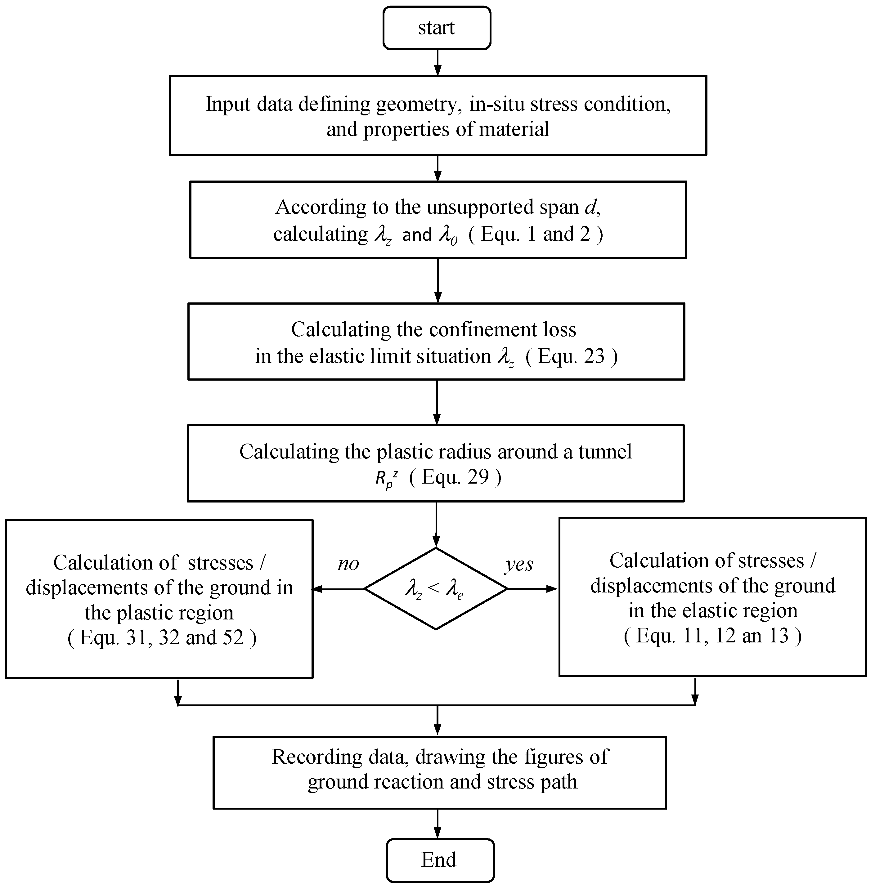
Calculation Steps in the Incremental Procedure Method

The incremental procedure employed in this study, also known as an explicit procedure, facilitates the conversion of analytical solutions into executable computations. These computations can be directly conducted using a calculation worksheet as depicted in Figure 6. Specifically, this paper introduces the explicit analysis method (EAM), capable of incorporating the confinement loss as an incremental step to simulate the progressive excavation of the tunnel. The EAM calculates stresses/displacements at each step and generates the ground reaction curve, the stress path at the intrados of the tunnel, and the distribution of stresses/displacements across tunnel cross-sections, as shown in Figure 7, the explicit algorithm process is used in the analysis of EAM.

The steps of calculation for the EAM are described by the following representations.

(1)

Input data: This relates to the data of the initial in situ stress, geometry of the tunnel, material properties, and unsupported distance.

(2)

To estimate the confinement loss λ_z at a certain distance z from the tunnel working face, one can use a given value of λ_z as a chosen effect of the unsupported distance of tunnel excavation. Therefore, λ_z can be determined from the Equation (1).

(3)

Dividing the confinement loss λ_z by n segments, the incremental step λ can be expressed as

$$∆\lambda ={\displaystyle \frac{1}{n}}\left(1-{\lambda }_z\right)$$

(56)

(4)

Calculating each step value of λ as

$$\begin{array}{cc}{\lambda }_{i+1}={\lambda }_z& i=0\\ {\lambda }_{i+1}={\lambda }_i+i\mathsf{\Delta }\lambda & i=1~\left(n-1\right)\end{array}$$

(57)

(5)

Attaining the final value ${\lambda }_n={\lambda }_{i+1}$

(6)

According to Equation (23), estimate the confinement loss in the elastic limit situation (λ_e).

(7)

If ${\lambda }_{i+1}<{\lambda }_e$, it means that the stress state is in the elastic region and that the radial and tangential stresses/displacements can be calculated with Equations (11)–(13).

(8)

If ${\lambda }_{i+1}\ge {\lambda }_e$, it means that the stress state is in the plastic region and that the plastic radius R_p can be calculated with Equation (29). Once one obtains this value R_p, the procedure automatically substitutes into Equations (31), (32) and (52) for the radial and tangential stresses, and the radial displacement, respectively.

(9)

Recording the calculated data relates to the representation of the distribution of stresses/displacements (${\displaystyle \frac{r}{R}},{\displaystyle \frac{{\sigma }_r}{{\sigma }_v}}$), (${\displaystyle \frac{r}{R}},{\displaystyle \frac{{\sigma }_{\theta }}{{\sigma }_v}}$), and (${\displaystyle \frac{r}{R}},{\displaystyle \frac{{2Gu}_r}{R{\sigma }_v}}$) on the cross-section of the tunnel and (${\displaystyle \frac{{2Gu}_r}{R{\sigma }_v}},{\displaystyle \frac{{\sigma }_r}{{\sigma }_v}}$) at the intrados of the tunnel.

(10)

When i < n − 1, repeat steps (4) through (10).

(11)

When i = n − 1, the process is not repeated, and the data from each step is recorded.

(12)

Drawing the distribution of stresses/displacements at the intrados and on the cross-section of the tunnel.

5. Comparison of Results between the Findings of This Study and Published Data

This study investigates case studies comparing the findings with published research such as Sharan and Naznin (2012) [41], alongside the EAM calculations conducted here. To assess the ground reaction resulting from tunnel excavation under unsupported conditions,

Table 1. Input data for the EAM computation utilizing published data.

Reference	Sharan and Naznin [41]
Parameter	Case I	Case II	Case III	Case IV	Case V
E (GPa)	60	90	40	5.5	27.6
ν	0.2	0.2	0.2	0.25	0.2
mi	10.84	16	7.5	17	15
GIS	89	90	79	50.08	50.31
D	0	0	0	0	0
σci (MPa)	210	200	300	30	69
Kψ	0	0	0	0	0
R (m)	10.0	10.0	4.0	5.0	6.1

presents the input data necessary for numerical calculations. Various case studies (Case I~III for the elastic region and Case IV~V for the plastic region) were examined to analyze the effects of different parameters on stress/displacement, dimensionless radial and tangential stresses, and dimensionless radial displacement. Table 1 outlines the properties of the rock masses, noting assumptions of zero dilation angle (K_ψ) and degree of disturbance (D) in this study. Additionally, the horizontal stress (σ_h) and vertical stress (σ_v) utilized in the calculations were 90 MPa and 135 MPa, respectively, resulting in a lateral stress ratio (K_o) of 0.67, describing the initial stress conditions of the tunnel excavated within anisotropic stress fields.

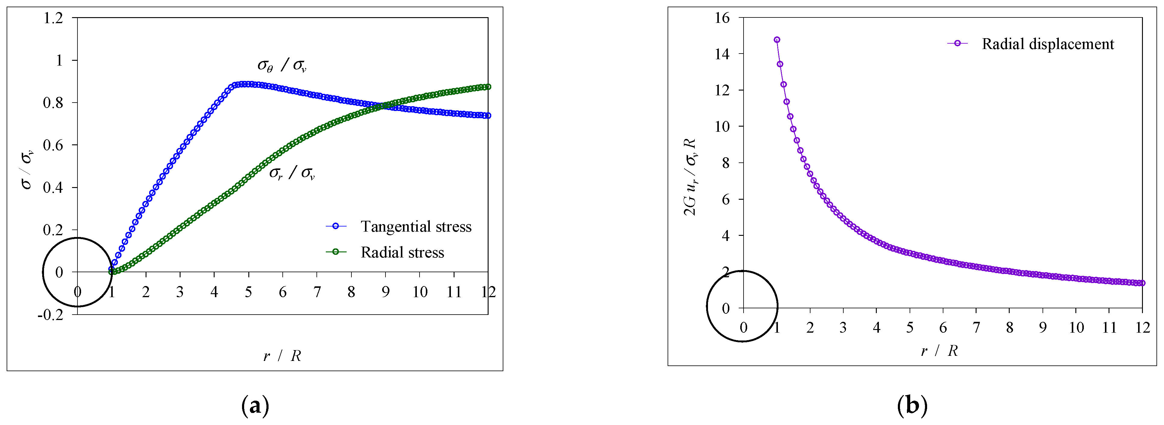
5.1. Stress/Displacement in the Elastic Region

In this paper, the dimensionless radial displacement (2Gu_r/Rσ_v), and radial and tangential stresses normalized by the vertical stress (σ_v) in the elastic region are plotted in Figure 8 and Figure 9. The behavior of rock masses at the intrados of the tunnel was altered by the advancing excavation of the tunnel face and may be interpreted by the ground reaction curve and the stress path at any point of the intrados of the tunnel. As shown in Figure 8, the results obtained by the EAM using the data of Case I indicate that the behavior of the rock masses presented linear elasticity in the ground reaction curve and the stress path. The calculated result is in agreement with the theoretical value that the dimensionless radial displacement was equal to 1.2 (Figure 8a), and the dimensionless radial and tangential stresses were equal to 0 and 1.0, respectively (Figure 8b). In addition, the circle at the origin of the coordinate system represents the size of the diameter of a circular tunnel in Figure 9.

Around a circular tunnel excavation in an anisotropic stress state, one is interested in the stress/displacement distribution over the tunnel cross-section. According to the stress distribution results of the tunnel, the following three stress states can be used to describe and verify the stress changes caused by the advancing excavation of the tunnel face:

(1)

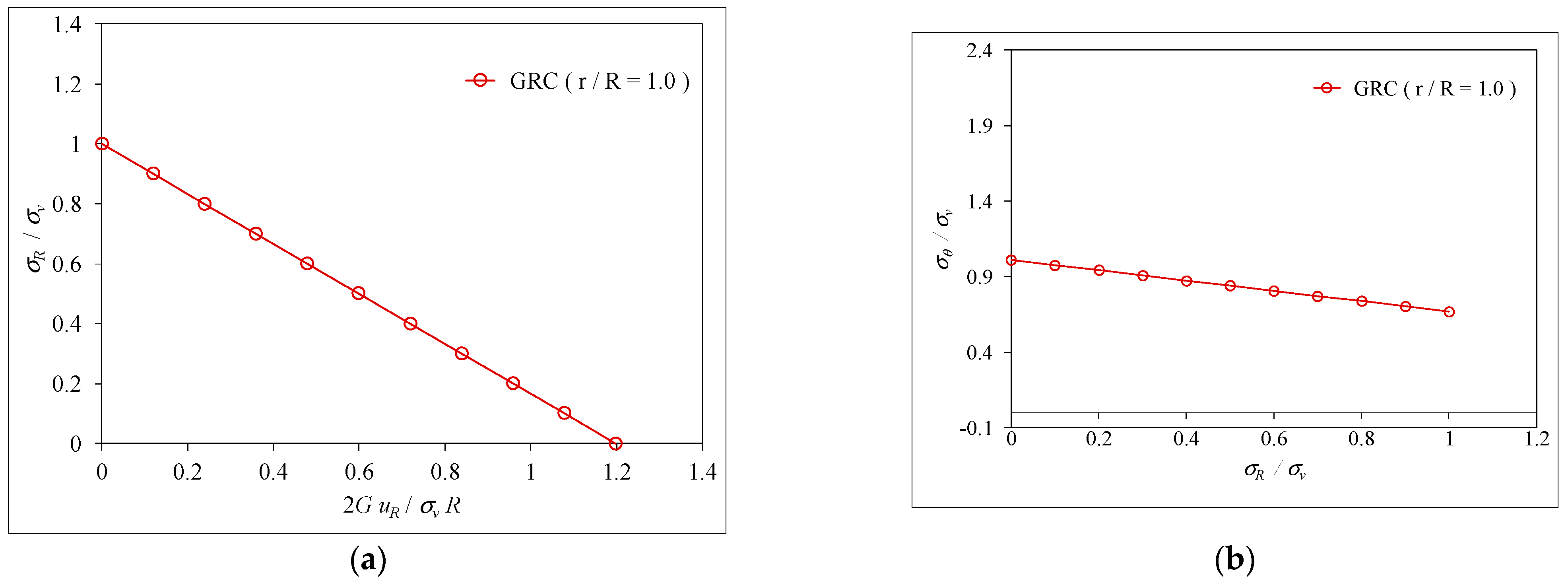
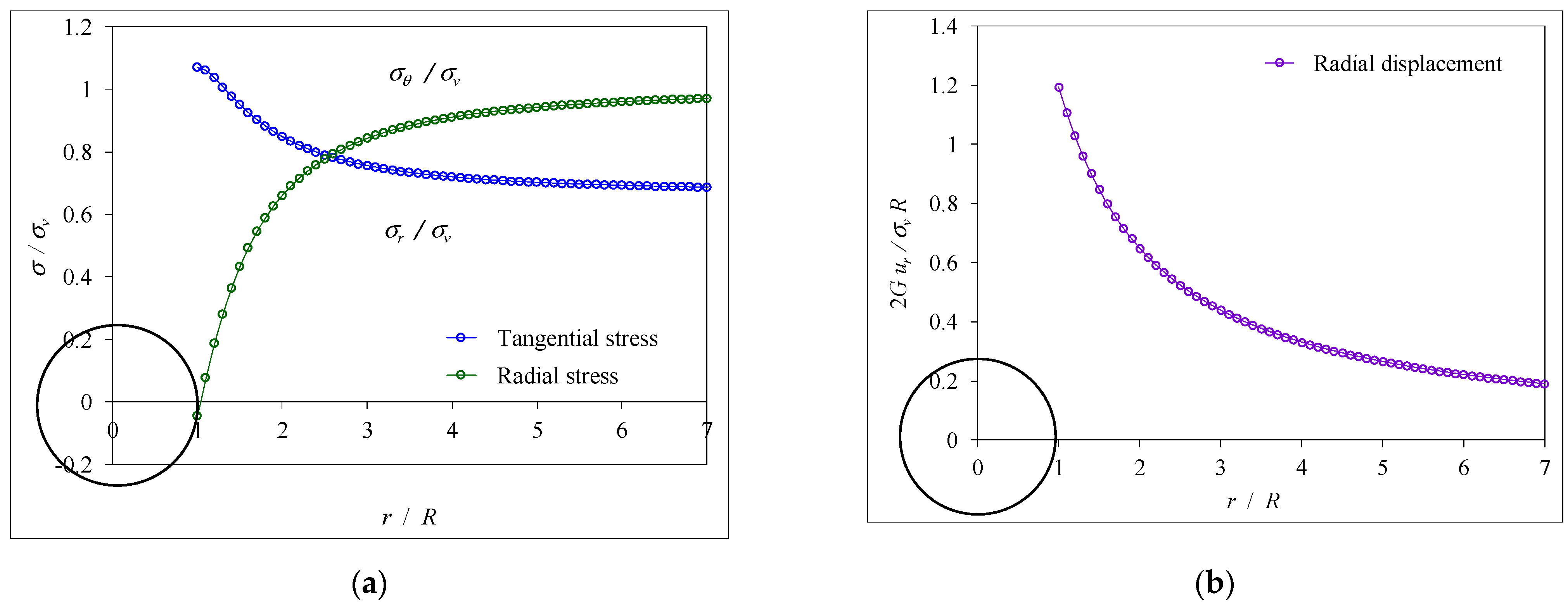
When λ = 0 ($r\to \infty$), it indicates that the dimensionless radial stress (σ_r/σ_v) and tangential stress (σ_θ/σ_v) used in the calculation were, respectively, 1 and 0.67 in the initial anisotropic stress state as shown the horizontal line on the right side in Figure 9a;

(2)

When 0 < λ < 1.0 ($R<r<\infty$), it describes that the stresses were also in the elastic region, the radial and tangential stresses increased with the increase of the confinement loss, and both stresses were separated along the horizontal axis (r/R);

(3)

When λ = 1.0 (r = R), the tangential stress attained the maximum value, and the radial stress equaled 0 as shown in Figure 9a. In addition, the distribution of radial displacement is given in Figure 9b.

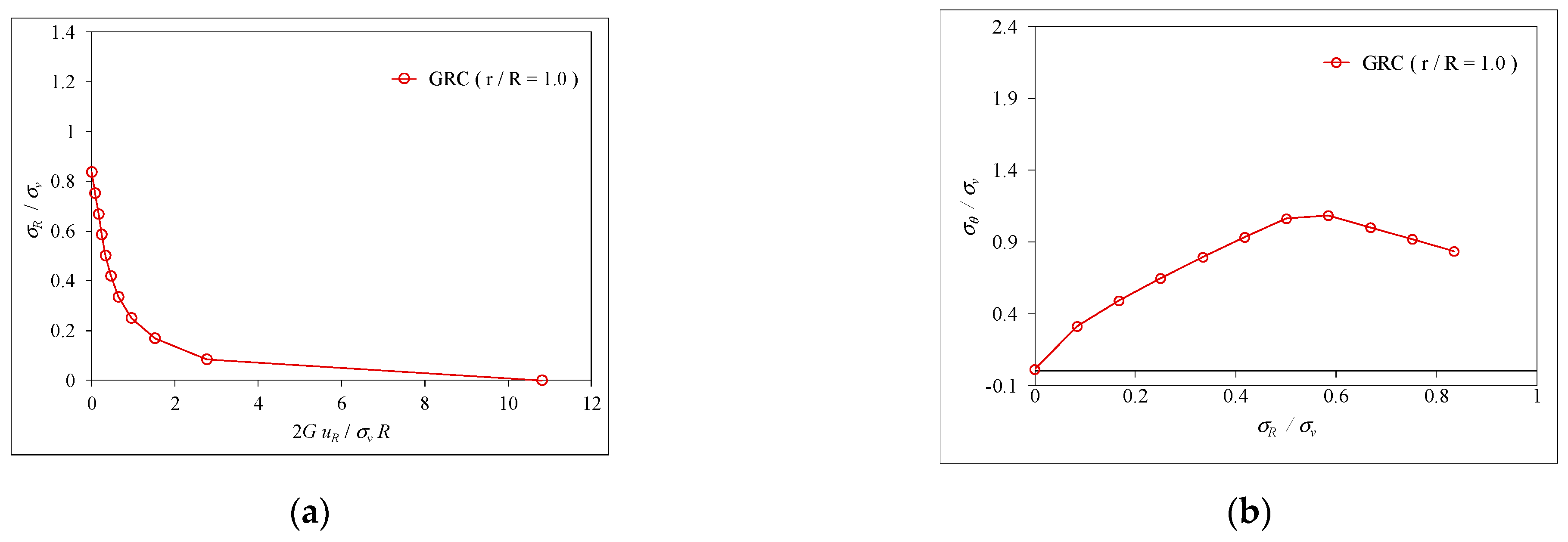
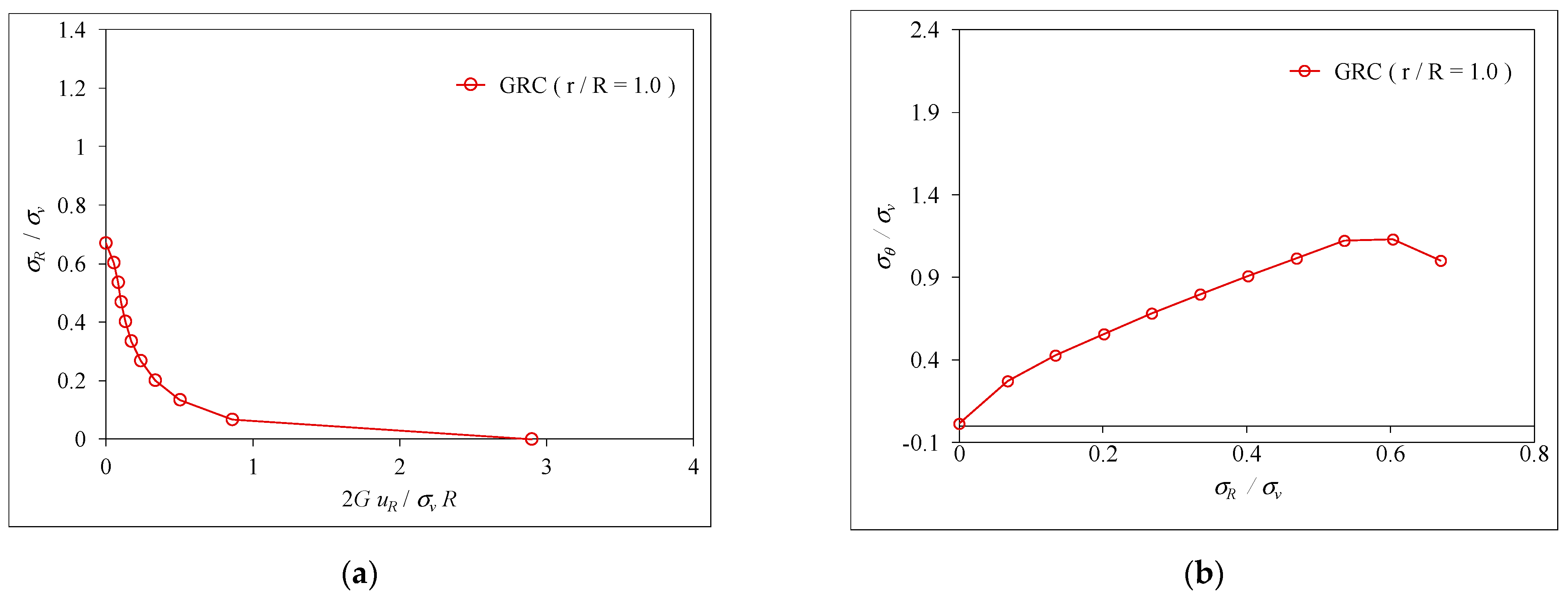
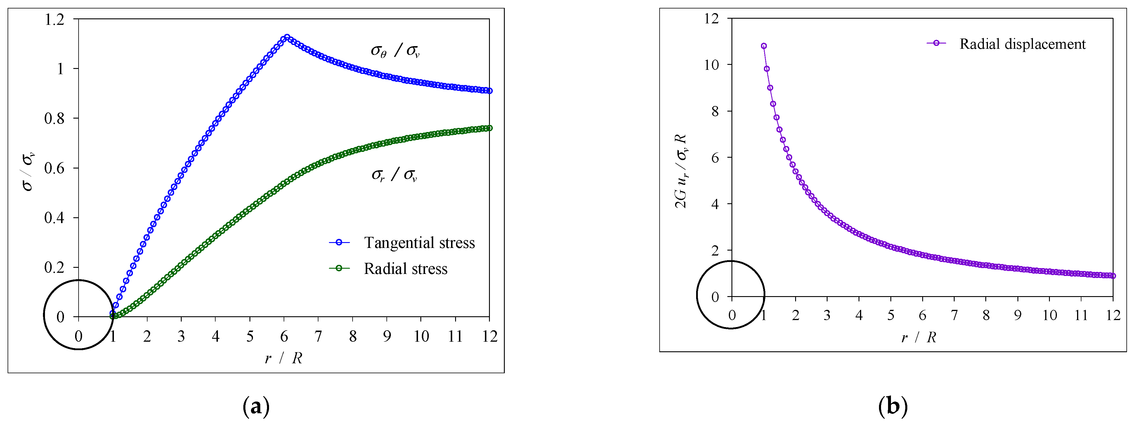
5.2. Stress/Displacement in the Plastic Region

Considering a circular tunnel excavation under anisotropic stress conditions, the key factor is the distribution of stress and displacement in the surrounding rock, particularly at the crown (θ = $0°$), inclination (θ = $45°$), and sidewall (θ = $90°$) of the tunnel. For stress and displacement at the tunnel intrados, the characteristic behavior in Case IV (about the plastic region) is illustrated in Figure 10a, Figure 11a and Figure 12a. These figures indicate that the rock masses exhibited non-linear elastic–perfectly plastic behavior in the ground reaction curve. Additionally, the dimensionless radial displacement is observed in the order of the crown, inclination, and sidewall of the tunnel.

As shown in Figure 1, the interface between the elastic region (line AB) and the plastic region (curve BC) is represented by point B. For the stress path, the Hoek–Brown failure criterion clearly demonstrated characteristic non-linearity along curve BG. In terms of the order in which the stress in the surrounding rock reaches the plastic state, the positions were the sidewall, inclination, and crown of the tunnel, as shown in Figure 10b, Figure 11b, and Figure 12b, respectively. The results obtained using the EAM under anisotropic stress conditions differed significantly from those obtained under isotropic stress fields.

For the distribution of stress/displacement on the cross-section of the tunnel in anisotropic stress fields, one is interested in the stress/displacement distribution over the tunnel cross-section. According to the stress distribution results of the tunnel, the following five stress states as shown in Figure 13a, Figure 14a, and Figure 15a can be used to describe and verify the stress changes caused by the advancing excavation of the tunnel face:

(1)

When λ = 0 ($r\to \infty$), it indicates that the stresses were in the initial stress state as shown in the horizontal line on the right side in Figures; the radial stress (σ_h/σ_v) and tangential stress (σ_θ/σ_v) used in the calculation were 0.67 and 1.0, respectively.

(2)

When 0$\le \lambda \le {\lambda }_e$ ($R_p\le r\le \infty$), it describes that the stresses were in the elastic region, and the radial and tangential stresses increased with the increase of the confinement loss, and both stresses were separated along the horizontal axis (r/R).

(3)

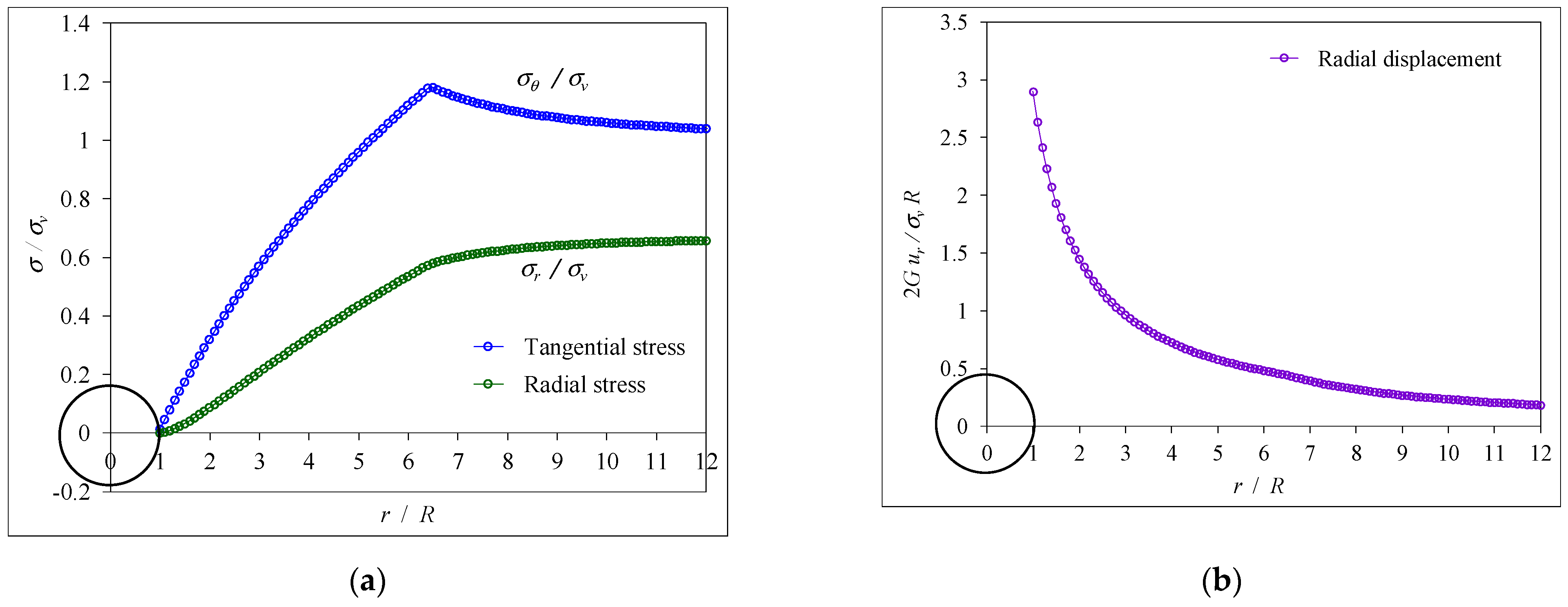
When $\lambda ={\lambda }_e$ ($r=R_p$), the plastic radius appeared, and stresses were at the elastic-plastic interface. The radial stress began to change the curvature, and the tangential stress attained the maximum value.

(4)

When ${\lambda }_e\le \lambda \le 1$ ($R\le r\le R_p$), it indicates that the stresses are in the plastic region, and this leads to both the radial stress and tangential stress being decreased steeply.

(5)

Until $\lambda =1$ ($r=R$), the radial stress becomes zero and the tangential stress is equal to the coefficient $\sqrt{4s{N}^2}$ proposed by the Hoek–Brown failure criterion.

According to the analysis results comparing the EAM with the listed articles (shown in

Table 2. Comparison of results between EAM and published data [41].

Published Studies	Radial Displacement, uR (m)	Plastic Zone Radius, Rp (m)	EAM Radial Displacement, uR (mm) (Error * %)	EAM Plastic Zone Radius, Rp (m) (Error * %)
Case I	0.09	N/A	0.0909 (1.0%)	N/A
Case II	0.05	N/A	0.0505 (0.93%)	N/A
Case III	0.11	N/A	0.1113 (1.18%)	N/A
Case IV	0.24	21.5	0.2268 (5.51%)	22.705 (5.60%)
Case V	0.038	14.3	0.0368 (3.28%)	15.014 (4.99%)

* $\mathrm{E}\mathrm{r}\mathrm{r}\mathrm{o}\mathrm{r}=\left|{\displaystyle \frac{\mathrm{p}\mathrm{u}\mathrm{b}\mathrm{l}\mathrm{i}\mathrm{s}\mathrm{h}\mathrm{e}\mathrm{d}\mathrm{d}\mathrm{a}\mathrm{t}\mathrm{a}-\mathrm{E}\mathrm{A}\mathrm{M}}{\mathrm{E}\mathrm{A}\mathrm{M}}}\right|\ast 100\%$.

), the percentage error for radial displacement ranged from 0.93% to 1.18% in the elastic region and from 3.28% to 5.51% in the plastic region. Additionally, the percentage error for the radius of the plastic zone ranged from 4.99% to 5.6%. When comparing the results calculated by the EAM in this study with published data, the approximate results align well with the observed trend. The analysis reveals that tunnels in anisotropic stress fields experience different failure mechanisms compared to those in isotropic fields. This has implications for the design and support systems of tunnels, suggesting that standard practices may need to be adjusted to account for anisotropic conditions.

6. Conclusions

Through the meticulous theoretical examination of the CCM of non-linear mechanical phenomena (utilizing the Hoek-Brown model) induced by tunnel excavation, coupled with the derivation of mechanical partial differential equations, development and application of an incremental calculation program of the EAM, and thorough comparison with existing findings, the following insights emerge:

(1)

A coherent closed-form analytical solution has been derived for the elastic–perfectly plastic analysis of a circular tunnel within rock masses governed by the Hoek–Brown non-linear failure criterion, considering anisotropic in situ stress.

(2)

The agreement between published results and the proposed closed-form solutions using the explicit procedure was excellent within elastic–perfectly plastic media. The percentage error for radial displacement ranged from 0.93% to 1.18% in the elastic region and from 3.28% to 5.51% in the plastic region. Additionally, the percentage error for the radius of the plastic zone ranged from 4.99% to 5.6%.

(3)

An incremental approach within the explicit analysis method (EAM) was proposed to model the advancing excavation of the tunnel face. This method calculates stresses and displacements at each step, facilitating the generation of ground reaction curves, stress paths at the intrados of the tunnel, and stress/displacement distributions across tunnel cross-sections.

(4)

The fluctuation of stresses during tunnel excavation can primarily be explained by the stress gradient, which represents the disparity between far-field and near-field stresses around the tunnel. This gradient can be computed using incremental assumptions in numerical analysis, with the confinement loss considered as a portion of the stress gradient.

(5)

Confinement loss in the elastic limit was determined by the peak strength parameters of the rock masses and initial vertical stress.

(6)

The plastic radius was influenced by the peak strength parameters of the rock masses, confinement loss in the elastic limit, and dependency on confinement loss. Increased confinement loss resulted in a larger plastic radius, reducing both radial and tangential stress while increasing radial displacement in the plastic region.

(7)

The incremental procedure method proposed herein accommodates the nonlinear failure criterion of the rock masses. It not only serves as a valuable tool for analyzing circular tunnels under isotropic stress conditions but also holds promise for simulating tunnel behavior under anisotropic stress conditions.

The innovative advantages of the analysis method proposed in this study are as follows: (1) the closed analytical solution of the ground reaction caused by tunnel excavation was rigorously derived through the mechanical model; (2) consideration conditions: stress presented various anisotropies, and the rock quality satisfied the nonlinear failure mode, (3) the direct calculation worksheet was used to complete the calculation of the analytical solution in an explicit method; (4) the approximate results of this study are presented quickly, directly, drawing, and conveniently.

The study underscores the necessity of incorporating anisotropic stress considerations into tunnel design and analysis. Using the Hoek–Brown failure criterion, engineers can achieve a more accurate and reliable assessment of tunnel stability, leading to safer and more efficient tunneling practices.

References

- Panet, M. Calcul du souténement des tunnels à section circulaire par la method convergence-confinement avec un champ de contraintes initiales anisotrope. Tunn. Et Ouvrages Souterr. 1986, 77, 228–232. [Google Scholar]
- Panet, M. Le Calcul des Tunnels par la Méthode de Convergence-Confinement; Presses de l’Ecole Nationale des Ponts et Chaussées: Paris, France, 1995. [Google Scholar]
- Panet, M. Recommendations on the Convergence-Confinement Method; Association Française des Tunnels et de l’Espace Souterrain (AFTES): Paris, France, 2001; pp. 1–11. Available online: https://tunnel.ita-aites.org/media/k2/attachments/public/Convergence-confinement%20AFTES.pdf (accessed on 28 September 2023).
- Panet, M.; Sulem, J. Convergence-Confinement Method for Tunnel Design; Springer: Berlin, Germany, 2022; Available online: https://link.springer.com/book/10.1007/978-3-030-93193-3 (accessed on 29 January 2023).
- Lee, Y.L.; Hsu, W.K.; Lee, C.M.; Xin, Y.X.; Zhou, B.Y. Direct calculation method for the analysis of non-linear behavior of ground-support interaction of circular tunnel using convergence–confinement approach. Geotech. Geol. Eng. 2021, 39, 973–990. [Google Scholar] [CrossRef]
- Lee, Y.L.; Hsu, W.K.; Chou, P.Y.; Hsieh, P.W.; Ma, C.H.; Kao, W.C. Verification and comparison of direct calculation method for the analysis of ground-support interaction of a circular tunnel excavation. Appl. Sci. 2022, 12, 1929. [Google Scholar] [CrossRef]
- Oreste, P.P. Analysis of structural interaction in tunnels using the convergence-confinement approach. Tunnell Undergr. Space Technol. 2003, 18, 347–363. [Google Scholar] [CrossRef]
- Oreste, P. The convergence–confinement method: Roles and limits in modern geomechanical tunnel design. Am. J. Appl. Sci. 2009, 6, 757–771. [Google Scholar] [CrossRef]
- Cui, L.; Zheng, J.; Zhang, R.; Lai, H. A numerical procedure for the fictitious support pressure in the application of the convergence-confinement method for circular tunnel design. Int. J. Rock Mech. Min. Sci. 2015, 78, 336–349. [Google Scholar] [CrossRef]
- Brown, E.; Bray, J.; Ladanyi, B.; Hoek, E. Ground response curves for rock tunnels. J. Geotech. Eng. ASCE 1983, 109, 15–39. [Google Scholar] [CrossRef]
- Brady, B.; Brown, E. Rock Mechanics for Underground Mining; Chapman & Hall: London, UK, 1993. [Google Scholar]
- Wang, Y. Ground response of a circular tunnel in poorly consolidated rock. J. Geotech. Eng. ASCE 1996, 122, 703–708. [Google Scholar] [CrossRef]
- Guan, Z.; Jiang, Y.; Tanabasi, Y. Ground reaction analyses in conventional tunnelling excavation. Tunnell Undergr. Space Technol. 2007, 22, 230–237. [Google Scholar] [CrossRef]
- Alejano, L.R.; Rodriguez-Dono, A.; Alonso, E.; Fdez-Manín, G. Ground reaction curves for tunnels excavated in different quality rock masses showing several types of post-failure behavior. Tunnell Undergr. Space Technol. 2011, 24, 689–705. [Google Scholar] [CrossRef]
- Mousivand, M.; Maleki, M.; Nekooei, M.; Msnsoori, M.R. Application of convergence-confinement method in analysis of shallow non-circular tunnels. Geotech. Geol. Eng. 2017, 35, 1185–1198. [Google Scholar] [CrossRef]
- Rocksupport. Rock Support Interaction and Deformation Analysis for Tunnels in Weak Rock; Tutorial Manual of Rocscience Inc.: Toronto, ON, Canada, 2004; pp. 1–76. [Google Scholar]
- Rodríguez, R.; Díaz-Aguado, M.B. Deduction and use of an analytical expression for the characteristic curve of a support based on yielding steel ribs. Tunnell Undergr. Space Technol. 2013, 33, 159–170. [Google Scholar] [CrossRef]
- Carranza-Torres, C.; Engen, M. The support characteristic curve for blocked steel sets in the convergence-confinement method of tunnel support design. Tunnell Undergr. Space Technol. 2017, 69, 233–244. [Google Scholar] [CrossRef]
- Oke, J.; Vlachopoulos, N.; Diederichs, M. Improvement to the convergence-confinement method: Inclusion of support installation proximity and stiffness. Rock Mech. Rock Eng. 2018, 51, 1495–1519. [Google Scholar] [CrossRef]
- De La Fuente, M.; Taherzadeh, R.; Sulem, J.; Nguyen, X.S.; Subrin, D. Applicability of the convergence-confinement method to full-face excavation of circular tunnels with stiff support system. Rock Mech. Rock Eng. 2019, 52, 2361–2376. [Google Scholar] [CrossRef]
- Lee, Y.L. Explicit analysis for the ground-support interaction of circular tunnel excavation in anisotropic stress fields. J. Chin. Inst Eng 2020, 43, 13–26. [Google Scholar] [CrossRef]
- Bernaud, D.; Rosset, G. The new implicit method for tunnel analysis. Int. J. Num. Anal. Meth. Geomech. 1996, 20, 673–690. [Google Scholar] [CrossRef]
- Humbert, P.; Dubouchet, A.; Fezans, G.; Remaud, D. CESAR-LCPC, un progiciel de calcul dédié au génie civil. Bull. Lab. Ponts Chaussées 2005, 256, 7–37. Available online: https://www.ifsttar.fr/collections/BLPCpdfs/blpc_256-257_7-37.pdf (accessed on 25 October 2023).
- González-Nicieza, C.; Álvarez-Vigil, A.E.; Menéndez-Díaz, A.; González-Palacio, C. Influence of the depth and shape of a tunnel in the application of the convergence-confinement method. Tunnell Undergr. Space Technol. 2008, 23, 25–37. [Google Scholar] [CrossRef]
- Vlachopoulos, N.; Diederichs, M. Improved longitudinal displacement profiles for convergence confinement analysis of deep tunnels. Rock Mech. Rock Eng. 2009, 42, 131–146. [Google Scholar] [CrossRef]
- Mousivand, M.; Maleki, M. Constitutive models and determining methods effects on application of Convergence-Confinement method in underground excavation. Geotech. Geol. Eng. 2017, 36, 1707–1722. [Google Scholar] [CrossRef]
- Zhao, K.; Bonini, M.; Debernardi, D.; Janutolo, M.; Barla, G.; Chen, G. Computational modelling of the mechanised excavation of deep tunnels in weak rock. Comput. Geotechics 2015, 66, 158–171. [Google Scholar] [CrossRef]
- Hoek, E.; Brown, E.T. Empirical strength criterion for rock masses. J Geotech. Eng. ASCE 1980, 106, 1013–1035. [Google Scholar] [CrossRef]
- Hoek, E.; Brown, E.T. Underground Excavations in Rock. CRC Press: London, UK, 1980. [Google Scholar]
- Hoek, E.; Carranza-Torres, C.; Corkum, B. Hoek–Brown failure criterion—2002 edition. Proc NARMS-Tac. 2020, 1, 267–273. Available online: https://static.rocscience.cloud/assets/verification-and-theory/RSData/Hoek-Brown-Failure-Criterion-2002-Edition.pdf (accessed on 1 January 2023).
- Carranza-Torres, C.; Fairhurst, C. The elasto-plastic response of underground excavations in rock masses that satisfy the Hoek–Brown failure criterion. Int. J. Rock Mech. Min. Sci. 1999, 36, 777–809. [Google Scholar] [CrossRef]
- Carranza-Torres, C.; Fairhurst, C. Application of the convergence-confinement method of tunnel design to rock masses that satisfy the Hoek–Brown failure criterion. Tunnell Undergr. Space Technol. 2000, 15, 187–213. [Google Scholar] [CrossRef]
- Carranza-Torres, C. Elasto-plastic solution of tunnel problems using the generalized form of the Hoek-Brown failure criterion. Int. J. Rock Mech. Min. Sci. 2004, 41, 480–491. [Google Scholar] [CrossRef]
- Sharan, S.K. Exact and approximate solutions for displacements around circular openings in elastic-brittle plastic Hoek-Brown rock. Int. J. Rock Mech. Min. Sci. 2005, 42, 542–549. [Google Scholar] [CrossRef]
- Park, K.H.; Kim, Y.J. Analytical solution for a circular opening in an elastic–brittle–plastic rock. Int. J. Rock Mech. Min. Sci. 2006, 43, 616–622. [Google Scholar] [CrossRef]
- Serrano, A.; Olalla, C.; Reig, I. Convergence of circular tunnels in elastoplastic rock masses with non-linear failure criteria and non-associated flow laws. Int. J. Rock Mech. Min. Sci. 2011, 48, 878–887. [Google Scholar] [CrossRef]
- Shen, B.; Barton, N. The disturbed zone around tunnels in jointed rock masses. Int. J. Rock Mech. Min. Sci. 1997, 34, 117–125. [Google Scholar] [CrossRef]
- Sharan, S.K. Elastic–brittle–plastic analysis of circular openings in Hoek–Brown media. Int. J. Rock Mech. Min. Sci. 2003, 40, 817–824. [Google Scholar] [CrossRef]
- Lee, Y.L.; Ma, C.H.; Lee, C.M. An improved incremental procedure for the ground reaction based on Hoek-Brown failure criterion in the tunnel convergence-confinement method. Mathematics 2023, 11, 3389. [Google Scholar] [CrossRef]
- Kirsch, G. Die Theorie der Elastizität und die Bedürfnisse der Festigkeitslehre: The theory of elasticity and the needs of the strength of materials. Z. Des Vereines Dtsch. Ingenieure 1898, 42, 797–807. [Google Scholar]
- Sharan, S.K.; Naznin, R. Linearization of the Hoek-Brown failure criterion for non-hydrostatic stress fields. In Proceedings of the Eighth International of the Conference on Engineering Computational Technology, Scotland, UK, 4–7 September 2012; Available online: https://webapp.tudelft.nl/proceedings/ect2012/pdf/sharan.pdf (accessed on 10 February 2023).