Abstract
This work is concerned with the study of explicit solutions for a generalized coupled nonlinear Schrödinger equations (NLS) system with variable coefficients. Indeed, by employing similarity transformations, we show the existence of rogue wave and dark–bright soliton-like solutions for such a generalized NLS system, provided the coefficients satisfy a Riccati system. As a result of the multiparameter solution of the Riccati system, the nonlinear dynamics of the solution can be controlled. Finite-time singular solutions in the norm for the generalized coupled NLS system are presented explicitly. Finally, an n-dimensional transformation between a variable coefficient NLS coupled system and a constant coupled system coefficient is presented. Soliton and rogue wave solutions for this high-dimensional system are presented as well.
Keywords:
coupled nonlinear Schrödinger equations; soliton solution; rogue wave solution; blow-up solution; similarity transformations; Riccati systems MSC:
81Q05; 35C05; 42A38
1. Introduction
The coupled nonlinear Schrödinger equation models several real phenomena such as the interaction of Bloch-wave packets in a periodic system [1], the evolution of two surface wave packets in deep water [2], and in wavelength-division-multiplexed systems [3]. The starting point of many studies of these kinds of models was the well-known Manakov system introduced in 1974 [4] (see Equations (3) and (4)). The Manakov system is an integrable coupled NLS characterized by equal nonlinear interactions within and between components [5]. A great effort has been made to figure out the dynamics of the soliton-like solutions for coupled NLS. Some of these structures are dark–bright (DB), bright–bright (BB), and dark–dark (DD) solitons. These states have been observed in several experiments in optics [6,7] and in the context of Bose–Einstein condensates [8]. Another important class of solutions is rogue waves. These types of solutions are strong wavelets that can appear in the ocean from nowhere and disappear without a trace. In fact, it is this particular property that makes them candidates for the study of predicting catastrophic phenomena such as tsunamis, thunderstorms, and earthquakes [9].
In order to describe some phenomena dynamics more realistically, the space–time variation of the coefficients must be taken into account in the majority of cases. In this sense, new nonlinear Schrödinger-type coupled systems with variable coefficients have been introduced [10,11,12,13,14,15,16,17,18,19,20]. The difficulty of obtaining non-constant coefficients in the construction of explicit solutions can be overcome by making use of different techniques such as the Hirota bilinear method [21,22], similarity transformations [13,16,20], Darboux transformations [10,11,23] and the Bäcklund transformation [24], to mention a few. These approaches have enabled the study of the existence and construction of non-trivial solutions for NLS models. We can specifically highlight the work [25], which effectively investigated the existence of non-trivial solutions for a superlinear Schrödinger model with sign-changing potential. The existence of singular solutions for NLS models has also been studied and reported in the literature; see for example [26,27].
During recent years and due to their many applications, there has been a growing interest in the study of solitons and rogue wave-type solutions for coupled variable coefficient NLS equations [12,15,17,18,19]. At present, the fields interested in these kinds of solutions and moved by the necessity of data transfer are optical fiber technology and soliton transmission. More precisely, these special solutions can overcome some difficulties related to physical properties of the fiber and the interaction of it and the transmitted soliton. Although some important advances have been made in understanding the dynamics of soliton solutions for generalized coupled NLS systems from the mathematical and physical point of view, it remains a difficult problem. In this context and under the revolution of hardware equipment and software technology, recent studies of these fascinating solutions have been carried out by using a deep learning approach as well [28,29].
In this work, the objective will be to study the Schrödinger-type coupled system with the quadratic Hamiltonian (VCNLS hereafter):
Here and represent complex wavefunctions, , , , , , , are given time-dependent functions, and . The coefficient is the dispersion management parameter, determines the time dependence of the quadratic potential, is the gain/loss term, standardizes an arbitrary linear potential, and is the nonlinear management. The system (1) and (2) appears to describe the propagation of solitons in birefringence fibers (see for example [13,20]), and also in the framework of solitary waves in multi-component Bose–Einstein condensates [30,31]. We point out that the proposed system (1) and (2) extends many of the models studied in the literature.
The uncoupled case () has been the source of many studies in the recent years [32,33,34,35]. By employing the similarity transformation and imposing the coefficients to satisfy a Riccati system (see Equations (19)–(24) and (58)–(63)), soliton-like solutions (bright, dark, and Peregrine), singular solutions, and the fundamental solution () were constructed. Also, the Riccati system allowed the construction and study of explicit solutions for diffusion-type equations [36] and reaction–diffusion equations [37].
This paper’s aim is to establish a relationship between dispersion, potential, damping, and nonlinearity terms by the Riccati system in order to obtain solutions such as dark–bright and rogue wave soliton solutions for the coupled VCNLS (1) and (2). The multiparameters solution of the Riccati system allows the soliton dynamics to be controlled; this is crucial in practice, because one needs to control the soliton transmission of information since standard vector solitons for NLS systems do not have controllable parameters. This relation in the coefficients provides the construction of solutions with blow-up in finite time in the norm. Finally, an n-dimensional generalization of the VCNLS is studied, and the existence of soliton solutions is shown as well.
This work makes the following contributions:
- It introduces a novel coupled system of Schrödinger equations with variable coefficients. In this regard, our work differs from the models explored in the literature, which typically do not take into account the dynamics of the solutions under the influence of dispersion, potential (linear and quadratic), damping, and nonlinear management all at once.
- It reports on new solitons, rogue waves, and singular solutions to coupled nonlinear Schrödinger systems with variable coefficients. The explicit construction of this important class of solutions demonstrates that coherent structures are possible in the presence of dispersion, potential, damping, and nonlinear management as long as the coefficients fulfill a Riccati system.
- It demonstrates the capacity to control solution dynamics using the Riccati system’s multiparametric solution. To the best of our knowledge, our approach is one of the few capable of analyzing this type of parameter influence. It could be meaningful for manipulating solitons experimentally.
The paper is organized as follows: in Section 2 we introduce the classical coupled Manakov system and its rogue wave and soliton-type solutions. The explicit construction of rogue wave and soliton-type solutions for the generalized coupled NLS system (1) and (2) is presented in Section 3. This objective is obtained by using Theorem 1 and solutions of the Manakov system given in the previous section. In Section 4, we construct explicit singular solutions for the generalized coupled NLS system, as can be seen in Theorem 2. Section 5 is devoted to the extension of the transformation established in Theorem 1. Such a new transformation allows us to connect an n-dimensional coupled NLS system with an n-dimensional Manakov system; see Theorem 3. Also, soliton and rogue wave solutions are constructed for this model. A Mathematica file has been prepared as Supplementary Materials, verifying the Riccati systems used in the construction of the solutions in all the previous sections. Conclusions and some final remarks are given in Section 6. Appendix A corresponds to the appendix, in which the solution of the Riccati system is presented.
2. Classical Solutions of Coupled NLS
The coupled NLS system, or Manakov system
is a nonlinear wave system that governs a wide variety of physical phenomena ranging from the dynamics of a two-component Bose–Einstein condensate [8,38], nonlinear optics [6,7], and the dynamics of deep-sea waves under the interaction of two-layer stratification [39]. This system (3) and (4) was shown by Manakov to be integrable [4,5]. It admits soliton-like structures such as dark–bright (DB) solutions. In fact, (3) and (4) possess DB solitons; see for example [6,8,10,20]:
where and are arbitrary constants. These kinds of solutions were first experimentally observed in photorefractive crystals [6]. Other interesting solutions with fascinating properties are rogue waves. Indeed, the coupled NLS system (3) and (4) admits the exact rogue wave solution of type I [10,20]:
where with The parameters with and , are arbitrary constants. Similarly, the rogue wave solution of type II [10,20] is given by:
where
In the subsequent section, we will use these solutions to construct explicit solutions for the generalized coupled NLS system.
3. Generalized Coupled NLS System
The aim of this section is to establish the existence of soliton-type and rogue wave solutions (by the explicit construction of these solutions) of the generalized coupled NLS system (1) and (2). More precisely, by using similarity transformations and by imposing the coefficients to satisfy the Riccati system, classical solutions of the standard Manakov system (3) and (4) are extended to this general framework. Indeed, the main result of this section is:
Theorem 1.
Let Then, the following NLS coupled system (or VCNLS)
admits dark–bright (DB) solitons and rogue wave-type solutions where satisfies the integrability condition with .
Proof.
Computing the first derivatives of the function (derivatives for are obtained by changing by ), we have
Therefore, equating each term to zero, and using the conditions , we deduce the well-known Riccati system [33,34,35,36]:
Now, considering the standard substitution (also obtained from equalizing to zero)
it follows that the Riccati Equation (19) becomes
with
We will refer to (26) as the characteristic equation of the Riccati system. From the last three terms on the left side of the equality (18), the functions and will satisfy the coupled NLS system in the new variables and :
where , , , , , and are given by Equations (A1)–(A13) set out in the Appendix A. Therefore, the existence of these kinds of solutions (DB and rogue wave solutions) are established by letting and be the solutions discussed in the previous section; see Equations (5)–(10). □
Remark 1.
3.1. Rogue Wave Solutions
The generation and behavior of rogue waves is a significant subject in oceanography. In this light, the solutions presented in this section may contribute to a better understanding of how this type of wave emerges as a result of a balance between dispersion, potential (quadratic and linear), damping, and nonlinearity.
The existence of rogue wave solutions for the model (11) and (12) can be guaranteed by the extension of solutions (7)–(10) by the previous Theorem 1, as will be seen in the following examples. Throughout the text, the coefficients are selected in such a way that the formulae corresponding to the solution of the Riccati system (A1)–(A13) provide explicit expressions. We start with the Type I rogue wave solutions.
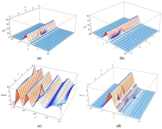
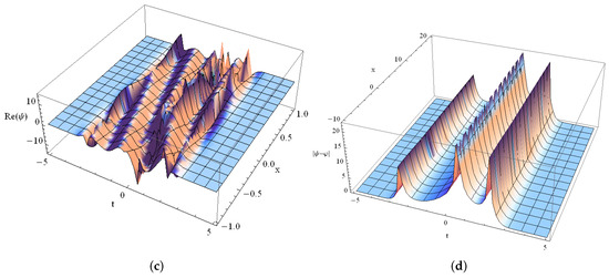
3.1.1. Case
In this scenario, we will look at the dynamics of the solutions when they are subjected to constant dispersion and damping, as well as exponential nonlinearities. The model has the form
Then, according to Theorem 1, we obtain
where is the confluent hypergeometric function given by the series with , and is the gamma function. Here, we have solved the Riccati system with the initial conditions , , , , , and
Therefore, we can construct a solution in the form:
where and are given by Equations (7) and (8). The profiles of these solutions for the parameters and are shown in Figure 1a,b. The real part of the function is displayed in Figure 1c. Figure 1d shows the difference between the two solutions to show that they are different.
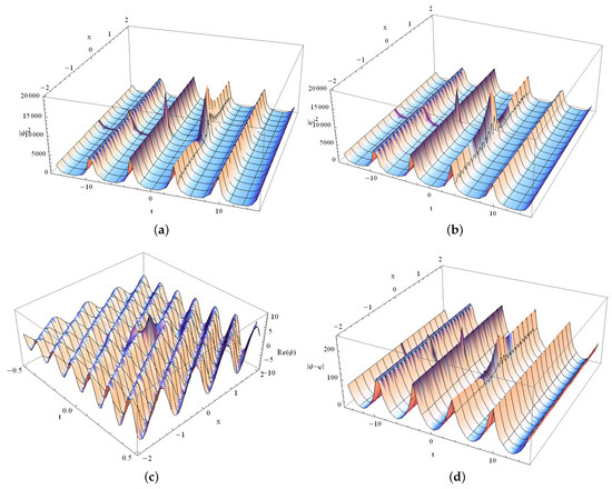
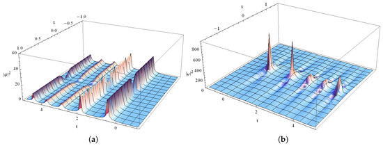
3.1.2. Case
This example demonstrates the existence of rogue wave solutions for a system without a quadratic potential but with periodic dispersion, constant damping, and exponential decay nonlinearities. In particular, the corresponding system is given by the equations
Then,
The initial conditions used to solve the Riccati system are the same as those given in the previous case. In fact, except for the section on bending dynamics, we shall use these initial conditions for the rest of the study. Solutions for the system (34) and (35) are
Again and are given by the Equations (7) and (8). Figure 2 shows the time evolution of and for the corresponding solutions. The difference between the two solutions are shown in the Figure 2c.
The next two cases correspond to the Type II rogue wave solutions.
3.1.3. Case , , , , ,
Assume the system
where is the Gudermannian function given by . The expressions for the functions , , , , , , and are
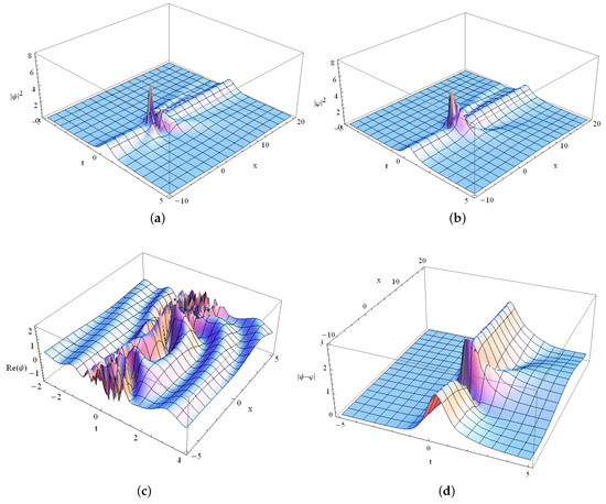
3.1.4. Case
Consider the system of the nonlinear Schrödinger equations
with . In this case, the solution of the Riccati system has the form
Then, by the assumption that and satisfy Equations (9) and (10), Theorem 1 provides the following solutions:
Figure 4 shows the profiles of for these particular solutions.
3.2. Dark–Bright Soliton-Type Solutions
This part of the work is concerned with the construction of solutions for the generalized coupled NLS system with soliton-type properties. As we will see, (11) and (12) admits DB-type solitons.
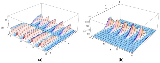
3.2.1. Case
This example illustrates how the dynamics of the soliton change when subjected to constant dispersion and damping. The associated system
admits the functions
In these terms, explicit solutions are given by the expressions
with and satisfying Equations (5) and (6).
Figure 5 shows the profiles of for these particular solutions.
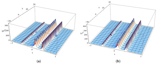
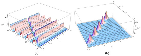
3.2.2. Case
Consider the system of nonlinear Schrödinger equations defined for
In Figure 6, we display the profiles of by using the values , , , and .
3.3. Bending Dynamics
In practice, many experiments are carried out in controlled surroundings, hence, it is important to have models that accurately replicate these types of conditions. In this sense, the purpose of this section is to demonstrate how the Riccati approach can be used to control the dynamics of solutions. As an example, we consider the system (50) and (51) again, but now, we change the initial conditions for and , i.e., ; and , . The , , and functions are now:
Figure 7, shows how these new parameters influence the system’s nonlinear dynamics: The propagation axis of the solutions is bended.
4. Blow-Up Solutions of the Generalized Coupled NLS System
The current section is focused on the study of singular solutions of the coupled VCNLS. More precisely, we demonstrate by explicit construction the existence of finite-time singular solutions in the norm.
Theorem 2
Proof.
We will proceed as in [33,34]. Substituting (56) and (57) into Equations (54) and (55) we obtain the modified Riccati system:
Here the previous system (58)–(63) differs from (19)–(24) by the extra term in Equation (63). Now, considering the substitution
it follows that the Riccati Equation (58) becomes
with
Using Equations (A1) and (A12) in the Appendix A with , (58)–(62) can be solved, but (63) must be solved separately. Let I be an interval such that for all Now, since the functions and are linearly independent on an interval , we have
and by given by (A1) (see [40]), functions (56) and (57) will have a finite time blow-up in the norm at , i.e.,
□
Remark 2.
The above theorem shows the possibility of obtaining singular solutions in for certain choices of the coefficients. In particular, the collapse time of the solutions corresponds to the instant where the function vanishes (if such time exists).
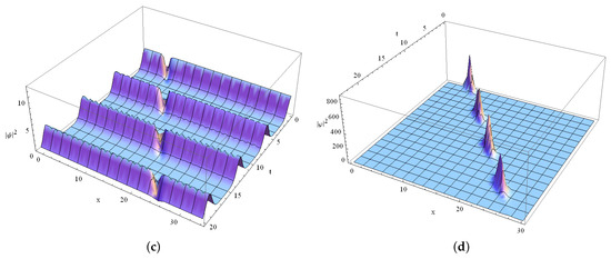
4.1. Case and Arbitrary h
Consider the coupled VCNLS system
Then, according to Theorem 2, the system admits the explicit solutions given by Equations (56) and (57) with the functions
Therefore,
and these solutions blow up in the norm at the instant , provided
The next example shows how a different coefficient selection alters the properties of these solutions (no blow-up). The function does not vanish at any point in time.
4.2. Case
Consider the coupled VCNLS system
In this case, we have
In this context, Theorem 2 allows us to extend the singular solutions established in Theorem 1 in [34] (see also Example 1 in the same reference).
5. An n-Dimensional Generalized Coupled NLS System
In Section 3, we established a relationship between the one-dimensional coupled VCNLS (11) and (12) and the well-known Manakov Equations (3) and (4), provided the coefficients satisfy the Riccati system (19)–(24). In the subsequent Section 4 and by “exploiting” the potential of the Riccati system, the construction of explicit singular solutions for (11) and (12) was shown. In this section, we reveal that a similar Riccati system (see Equations (81)–(86)) allows us to link an n-dimensional coupled NLS system with a generalized Manakov system. It will be useful in constructing soliton solutions for the high-dimensional system.
Theorem 3.
The nonautonomous coupled NLS n-dimensional
with and can be transformed into the standard coupled NLS
by the transformations
with for and Additionally, the following Riccati system is satisfied
Considering the substitution
it follows that the Riccati Equation (81) becomes
In general, the study of n-dimensional coupled NLS systems is carried out by degenerating them into the one-dimensional coupled NLS ()see for example [41,42] for the two-dimensional case), or directly dealing with the high-dimensional system, as can be seen in [43] for . In contrast, our transformation does not reduce the spatial dimension of the system, and then, to find soliton solutions for (75) and (76) in terms of Theorem 3, we used the ideas given in the works [41,42,43].
5.1. Case
5.2. Case
Consider the three-dimensional coupled NLS system
6. Conclusions and Final Remarks
Through this current work, we proposed and showed the integrability of a generalized coupled VCNLS (containing a dispersion coefficient, potential, damping, and nonlinear coefficient) using the similarity transformation established in Theorems 1 and 3. Here, the Riccati system played a crucial role in the explicit construction of soliton-type solutions, rogue waves, and singular solutions for these kinds of equations. The explicit construction of soliton and rogue wave-type solutions for an n-dimensional coupled NLS system was shown as well. We show solutions with striking characteristics (with the possibility of applications) and the ability to control their propagation dynamics.
On the other hand, even if the solutions reported in this work lacked physical application, they are an important input for the study of the precision and stability of the numerical methods applied to these models. Whatever the case, this work should motivate further analytical and numerical studies looking to clarify the connections between the dynamics of variable-coefficient NLS and the dynamics of Riccati systems. Finally, we hope that this fresh approach to dealing with VCNLS systems will provide new insights into the physics of such models and aid in comprehending real-world applications.
Supplementary Materials
A mathematica file verifying the Riccati system used in the construction of the solutions can be found at: https://www.mdpi.com/article/10.3390/math12172694/s1.
Author Contributions
Investigation, J.M.E. and E.S.; Writing—original draft, J.M.E. and E.S.; Writing—review & editing, J.M.E. and E.S. All authors have read and agreed to the published version of the manuscript.
Funding
This research received no external funding.
Data Availability Statement
No new data were created or analyzed in this study. Data sharing is not applicable to this article.
Acknowledgments
The authors thank the anonymous reviewers for their valuable time spent reading our work.
Conflicts of Interest
The authors declare no conflict of interest.
Appendix A. Solution of the Riccati System
In this appendix, we provide a solution of the Riccati system (19)–(24), and we point out that all the formulas involved in such a solution have been verified previously in [44]. A solution of the Riccati system with multiparameters is given by the following expressions (with the respective inclusion of the parameter ) [33,34,45]:
subject to the initial arbitrary conditions , , , , , , and . , , , , , and are given explicitly by
with Here and represent the fundamental solution of the characteristic equation subject to the initial conditions , , and , .
References
- Shi, Z.; Yang, J. Solitary waves bifurcated from Bloch-band edges in two-dimensional periodic media. Phys. Rev. E 2007, 75, 056602. [Google Scholar] [CrossRef] [PubMed]
- Roskes, G. Some Nonlinear multiphase interactions. Stud. Appl. Math. 1976, 55, 231–238. [Google Scholar] [CrossRef]
- Menyuk, C. Stability of solitons in birefringent optical fibers. Opt. Fibers J. Opt. Soc. Am. B 1998, 5, 392–402. [Google Scholar] [CrossRef]
- Manakov, S.V. On the theory of two-dimensional stationary self-focusing of electromagnetic waves. Zhurnal Eksperimentalnoi Teor. Fiz. 1973, 65, 505–516. [Google Scholar]
- Zakharov, V.E.; Schulman, E.I. To the Integrability of the system of Two coupled Nonlinear Schrödinger Equations. Physica D 1982, 4, 270–274. [Google Scholar] [CrossRef]
- Chen, Z.; Segev, M.; Coskun, T.; Christodoulides, D.; Kivshar, Y. Coupled photorefractive spatial-soliton pairs. J. Opt. Soc. Am. B 1997, 14, 2066–3077. [Google Scholar] [CrossRef]
- Ostrovskaya, E.; Kivshar, Y.; Chen, Z.; Segev, M. Interaction between vector solitons and solitonic gluons. Opt. Lett. 1999, 24, 327–329. [Google Scholar] [CrossRef]
- Busch, T.; Anglin, J.R. Dark-Bright Solitons in Inhomogeneous Bose-Einstein Condensates. Phys. Rev. Lett. 2001, 87, 010401. [Google Scholar] [CrossRef]
- Akhmediev, N.; Ankiewicz, A.; Soto-Crespo, J. Rogue waves and rational solutions of the nonlinear Schrödinger Equation. Phys. Rev. E 2009, 80, 026601. [Google Scholar] [CrossRef]
- Bo-Ling, G.; Li-Ming, L. Rogue wave, Breathers and Bright-Dark-Rogue Solutions for the Coupled Schrödinger Equations. Chin. Phys. Lett. 2011, 28, 110202. [Google Scholar]
- Du, Z.; Tian, B.; Chai, H.P.; Sun, Y.; Zhao, X.H. Rogue waves for the coupled variable-coefficient fourth-order nonlinear Schrödinger equations in an inhomogeneous optical fiber. Chaos Solitons Fractals 2018, 109, 90–98. [Google Scholar] [CrossRef]
- El-Shiekh, R.M.; Gaballah, M. Solitary wave solutions for the variable-coefficient coupled nonlinear Schrödinger equations and Davey–Stewartson system using modified sine-Gordon equation method. J. Ocean. Eng. Sci. 2020, 5, 180–185. [Google Scholar] [CrossRef]
- Han, L.; Huang, Y.; Liu, H. Solitons in coupled nonlinear Schrödinger equations with variable coefficients. Commun. Nonlinear Sci. Numer. Simul. 2014, 19, 3063–3073. [Google Scholar] [CrossRef]
- Kevrekidis, P.G.; Frantzeskakis, D.J. Solitons in coupled nonlinear Schrödinger models: A survey of recent developments. Rev. Phys. 2016, 1, 140–153. [Google Scholar] [CrossRef]
- Liu, X.; Zhou, Q.; Biswas, A.; Alzahrani, A.K.; Liu, W. The similarities and differences of different plane solitons controlled by (3 + 1)-Dimensional coupled variable coefficient system. J. Adv. Res. 2020, 24, 167–173. [Google Scholar] [CrossRef]
- Manganaro, N.; Parker, D.F. Similarity reductions for variable-coefficient coupled nonlinear Schrödinger equations. J. Phys. A Math. Gen. 1993, 26, 4093–4106. [Google Scholar] [CrossRef]
- Ozisik, M.; Secer, A.; Bayram, M. On the examination of optical soliton pulses of Manakov system with auxiliary equation technique. Optik 2022, 268, 169800. [Google Scholar] [CrossRef]
- Pashrashid, A.; Gomez, C.A.; Mirhosseini-Alizamini, S.M.; Motevalian, S.N.; Albalwi, M.D.; Ahmad, H.; Yao, S.W. On travelling wave solutions to Manakov model with variable coefficients. Open Phys. 2023, 21, 20220235. [Google Scholar] [CrossRef]
- Qiu, Y.; Gao, P. New Exact Solutions for the Coupled Nonlinear Schrödinger Equations with Variable Coefficients. J. Appl. Math. Phys. 2020, 8, 1515–1523. [Google Scholar] [CrossRef]
- Yu, F.; Yan, Z. New rogue waves and dark-bright soliton solutions for a coupled nonlinear Schrödinger equation with variable coefficients. Appl. Math. Comput. 2014, 233, 351–358. [Google Scholar] [CrossRef]
- Chakraborty, S.; Nandy, S.; Barthakur, A. Bilinearization of the generalized coupled nonlinear Schrödinger equation with variable coefficients and gain and dark-bright pair soliton solutions. Phys. Rev. E 2015, 91, 023210. [Google Scholar] [CrossRef] [PubMed]
- Zhang, L.L.; Wang, X.M. Bright–dark soliton dynamics and interaction for the variable coefficient three-coupled nonlinear Schrödinger equations. Mod. Phys. Lett. B 2019, 34, 2050064. [Google Scholar] [CrossRef]
- Chai, J.; Tian, B.; Chai, H.P. Darboux transformation and vector solitons for a variable-coefficient coherently coupled nonlinear Schrödinger system in nonlinear optics. Opt. Eng. 2016, 55, 116113. [Google Scholar] [CrossRef]
- Chai, J.; Tian, B.; Zhen, H.L.; Sun, W.R.; Liu, D.Y. Bright and dark solitons and Bäcklund transformations for the coupled cubic-quintic nonlinear Schrödinger equations with variable coefficients in an optical fiber. Phys. Scr. 2015, 90, 045206. [Google Scholar] [CrossRef]
- Chen, W.; Wu, Y.; Jhang, S. On nontrivial solutions of nonlinear Schrödinger equations with sign-changing potential. Adv. Differ. Equ. 2021, 232, 1–10. [Google Scholar] [CrossRef]
- Li, J.; Wang, Y. Nonexistence and existence of positive radial solutions to a class of quasilinear Schrödinger equations in RN. Bound. Value Probl. 2020, 81, 1–14. [Google Scholar]
- Wu, M.; Yang, Z. Existence of boundary blow-up solutions for a class of quasiliner elliptic systems for the subcritical case. Commun. Pure Appl. Anal. 2007, 6, 531–540. [Google Scholar] [CrossRef]
- Pu, J.C.; Chen, Y. Data-driven vector localized waves and parameters discovery for Manakov system using deep learning approach. Chaos Solitons Fractals 2022, 160, 112182. [Google Scholar] [CrossRef]
- Raissi, M.; Perdikaris, P.; Karniadakis, G. Physics-informed neural networks: A deep learning framework for solving forward and inverse problems involving nonlinear partial differential equations. J. Comput. Phys. 2019, 378, 686–707. [Google Scholar] [CrossRef]
- Ho, T.L.; Shenoy, V.B. Binary Mixtures of Bose Condensates of Alkali Atoms. Phys. Rev. Lett. 1996, 77, 3276–3279. [Google Scholar] [CrossRef]
- Timmermans, E. Phase Separation of Bose-Einstein Condensates. Phys. Rev. Lett. 1998, 81, 5718–5721. [Google Scholar] [CrossRef]
- Amador, G.; Colon, K.; Luna, N.; Mercado, G.; Pereira, E.; Suazo, E. On Solutions for Linear and Nonlinear Schrödinger Equations with Variable Coefficients: A Computational Approach. Symmetry 2016, 8, 38. [Google Scholar] [CrossRef]
- Cordero-Soto, R.; Lopez, R.; Suazo, E.; Suslov, S. Propagator of a charged particle with a spin in uniform magnetic and perpendicular electric fields. Lett. Math. Phys. 2008, 84, 159–178. [Google Scholar] [CrossRef]
- Escorcia, J.; Suazo, E. Blow-up results and soliton solutions for a generalized variable coefficient nonlinear Schrödinger equation. Appl. Math. Comput. 2017, 301, 155–176. [Google Scholar] [CrossRef]
- Suazo, E.; Suslov, S.K. Soliton-like Solutions for the Nonlinear Schrödinger Equation with Variable quadratic Hamiltonians. J. Russ. Laser Res. 2012, 33, 63–83. [Google Scholar] [CrossRef]
- Suazo, E.; Suslov, S.K.; Vega-Guzmán, J.M. The Riccati System and a Diffusion-Type Equation. Mathematics 2014, 2, 96–118. [Google Scholar] [CrossRef]
- Pereira, E.; Suazo, E.; Trespalacios, J. Riccati–Ermakov systems and explicit solutions for variable coefficient reaction–diffusion equations. Appl. Math. Comput. 2018, 329, 278–296. [Google Scholar] [CrossRef]
- Kevrekidis, P.; Frantzeskakis, D.; Carretero-Gonzalez, R. Emergent Nonlinear Phenomena in Bose-Einstein Condensates: Theory and Experiment; Springer: Berlin/Heidelberg, Germany, 2008. [Google Scholar]
- Yilmaz, E.U.; Khodad, F.S.; Ozkan, Y.S.; Abazari, R.; Abouelregal, A.E.; Shaayesteh, M.T.; Rezazadeh, H.; Ahmad, H. Manakov model of coupled NLS equation and its optical soliton solutions. J. Ocean. Eng. Sci. 2022, 9, 364–372. [Google Scholar] [CrossRef]
- Cordero-Soto, R.; Suslov, S. The degenerate parametric oscillator and Ince’s equation. J. Phys. A Math Theor. 2011, 44, 015101. [Google Scholar] [CrossRef]
- Lan, Z.Z.; Gao, B.; Du, M.J. Dark solitons behaviors for a (2+1)-dimensional coupled nonlinear Schrödinger system in an optical fiber. Chaos Solitons Fractals 2018, 111, 169–174. [Google Scholar] [CrossRef]
- Manikandan, K.; Senthilvelan, M.; Kraenkel, R.A. On the characterization of vector rogue waves in two-dimensional two coupled nonlinear Schrödinger equations with distributed coefficients. Eur. Phys. J. B 2016, 89, 218. [Google Scholar] [CrossRef]
- Lan, Z.Z. Dark solitonic interactions for the (3 + 1)-dimensional coupled nonlinear Schrödinger equations in nonlinear optical fibers. Opt. Laser Technol. 2019, 113, 462–466. [Google Scholar] [CrossRef]
- Koutschan, C.; Suazo, E.; Suslov, S.K. Fundamental laser modes in paraxial optics: From computer algebra and simulations to experimental observation. Appl. Phys. B 2015, 121, 315–336. [Google Scholar] [CrossRef]
- Suslov, S.K. On integrability of nonautonomous nonlinear Schrödinger equations. Am. Math. Soc. 2012, 140, 3067–3082. [Google Scholar] [CrossRef]


Disclaimer/Publisher’s Note: The statements, opinions and data contained in all publications are solely those of the individual author(s) and contributor(s) and not of MDPI and/or the editor(s). MDPI and/or the editor(s) disclaim responsibility for any injury to people or property resulting from any ideas, methods, instructions or products referred to in the content. |
© 2024 by the authors. Licensee MDPI, Basel, Switzerland. This article is an open access article distributed under the terms and conditions of the Creative Commons Attribution (CC BY) license (https://creativecommons.org/licenses/by/4.0/).