Homogeneity Test of Ratios of Two Proportions in Stratified Bilateral and Unilateral Data

Abstract

In paired-organ studies such as ophthalmology, otolaryngology, and rheumatology, etc., various approaches take highly correlated bilateral data into account for homogeneity tests but are less likely to focus on combined bilateral and unilateral data structures. Also, it is necessary and important to adjust the effect of confounders on stratified combined bilateral and unilateral data since, in these data structures, ignoring intra-class correlation and confounding effects can cause biased statistical inference. This article derived three homogeneity tests (the likelihood ratio test, the Wald test, and the score test) concerning these cooperative structure data to detect if ratios of proportions retain consistency across strata. Simulation shows that the score test provides a robust Type I error rate and satisfactory power performance. Finally, a real example is applied to demonstrate the application of these three proposed tests.

1. Introduction

Paired bilateral data occur naturally in clinical trial studies, especially in ophthalmology, otolaryngology, and rheumatology, etc. Numerous clinical trials in ophthalmology widely utilize data collection involving one or both eyes [1]. In these scenarios, each subject may contribute either bilaterally or unilaterally, resulting in the data structure being bilateral and unilateral data existing simultaneously. Also, in practice, to determine the effect of exposure, some clinical trial procedures desire to stratify the data to avoid confounding by stratifying two or more categories in subgroups, aiming to obtain unbiased treatment effects. Estimating the effect of exposure can be biased if the investigator fails to adjust for stratified factors when analyzing the homogeneity test during trials.

Data were stratified by some control variables such as location, age, gender, etc., to detect whether the inference we were interested in involved treatment-by-stratum interaction. In the stratified sample design with two groups, the homogeneity test concerning proportions ratios is often referred to as inspecting if relative risk maintains the same across strata. When the ratio of proportions in the two groups is significantly different, we can include a confounding effect. If homogeneity is claimed, stratified data can be combined in a pooled dataset to investigate statistical inference. Therefore, it was necessary and important that we applied a homogeneity test to the stratified clinical data.

We investigated three homogeneity test methods of ratios of proportions on stratified unilateral and bilateral data structures in two groups. For unilateral cases, the homogeneity test can be treated as independent and applied by a usual method that has been studied in detail and thoroughly in the literature [2]. Naturally, two eyes in the same patient tend to be highly correlated in bilateral cases [3]. Without considering such a situation, standard inference and test methods may produce misleading statistical significance and inadequate power. Previous studies have explored models specially designed to address intraclass correlated data. Rosner introduced an approach referred to as the “constant R model” with the assumption that dependence between two paired organs of the same subject is measured as a constant R. Tang et al. [4], Ma et al. [5], Shan and Ma [6], and Liu et al. [7] then developed related asymptotic and exact test methods based this model. Afterward, Dallal [8] pointed out that the “Constant R model” could have poor performance on compound multinomial sampling and then provided a new approach with the assumption that the conditional probability of one eye given the other eye in the same person is not connected to the probabilities of the individual in the general population. Donner [9] introduced a widely used model under the assumption that the intraclass correlation coefficient, denoted as “$\rho$”, is generally considered uniform across groups. The model, along with an adjusted chi-square test, has been further validated in subsequent studies ([10,11,12]). Additionally, asymptotic and exact testing methods ([7,13,14,15]) have been explored in later research. In this paper, we incorporate Donner’s $\rho$ model since the $\rho$ model can also be applied to an arbitrary number of units provided by an individual.

Statistical data analysis focusing on stratified data also has been extensively studied in clinical trials. Lui and Kelly [16] focused on the homogeneity test of risk difference in unilateral cases and then discussed sparse data with a bootstrap method to improve the power of previous test designs. Li and Tang [17] applied the $\rho$ model to fit stratified matched-pair studies to develop computationally effective score test statistics. Tang and Qiu [18] conducted the homogeneity test for risk difference under Rosner’s R model. Then, Pei et al. [19], based on Donner’s model, explored homogeneity tests on stratified bilateral data. However, several issues have been raised here, considering the combined data structure. The aforementioned stratified data test methods only consider bilateral cases. Therefore, to evaluate treatment effectiveness in these scenarios, unilateral and bilateral cases occurred simultaneously. We further analyze and develop bilateral test methods appropriate to the combined data structure. In this paper, our goal is to develop new statistical test methods aiming to evaluate the homogeneity of the ratio of proportions across strata under a combined data structure without the assumption of a common ratio.

The remainder of this article is structured as follows. Section 2 derives both constrained and unconstrained maximum likelihood estimates for the parameters and examines three different testing procedures: the likelihood ratio test, the Wald test, and the score test. Section 3 presents Monte Carlo simulation studies designed to assess the performance of these tests in terms of empirical Type I error rates and statistical power. Section 4 provides an application of the methodologies to a real data example. Finally, Section 5 provides conclusions and remarks.

2. Methods

Suppose there are J strata, and for each stratum, there are $M=\sum M_j$ patients, which provide bilateral records and $N=\sum N_j$ patients, which provide unilateral records in g groups, $g=1,2$. $m_{lij}$ represents the number of patients having l responses ($l=0,1,2$) in the ith group ($i=1,2$) of the jth stratum ($j=1,2,\dots ,J$). $m_{l+j}$ is the total number of patients having l responses among all groups, and $m_{+ij}$ is the total number of patients in the ith group. The same notations are also applied to the unilateral case. The data structure of the jth stratum is summarized in Table 1.

Table 1. Data structure for the jth stratum in the stratified unilateral and bilateral cases.

	Group (i)
Number of Responses in Event	1	2	Total
0	$m_{01j}$	$m_{02j}$	$m_{0+j}$
1	$m_{11j}$	$m_{12j}$	$m_{1+j}$
2	$m_{21j}$	$m_{22j}$	$m_{2+j}$
Total	$m_{+1j}$	$m_{+2j}$	$M_j$
0	$n_{01j}$	$n_{02j}$	$n_{0+j}$
1	$n_{11j}$	$n_{12j}$	$n_{1+j}$
Total	$n_{+1j}$	$n_{+2j}$	$N_j$

For the bilateral case, we denote $Z_{ijhk}=1$ as an event that the kth eye ($k=1,2$) of the hth patient in the ith treatment group from the jth stratum has an expected response, cured or effected, $Z_{ijhk}=0$ otherwise. Since we applied Donner’s $\rho$ model here, it assumes that the correlations of response between two eyes are the same across all individuals in the two groups from a single stratum but can be different in different strata. Hence, for a given j stratum, we can express Donner’s model as $P(Z_{ijhk}=1)={\pi }_{ijk}$, ${\pi }_{ij1}={\pi }_{ij2}={\pi }_{ij}$; $Corr(Z_{ijh1},Z_{ijh2})={\rho }_j,-1\le {\rho }_j\le 1$, where ${\pi }_{ij}$ is the ith group proportion in the jth stratum that has an expected event, and ${\rho }_j$ is the common correlation of the jth stratum. Then, the probabilities of an expected response for none, one, or both eyes are as follows:

$$\begin{array}{cc}\hfill p_{0ij}& ={\rho }_j(1-{\pi }_{ij})+(1-{\rho }_j){(1-{\pi }_{ij})}^2,\hfill \\ \hfill p_{1ij}& =2{\pi }_{ij}(1-{\rho }_j)(1-{\pi }_{ij}),\hfill \\ \hfill p_{2ij}& ={\rho }_j{\pi }_{ij}+(1-{\rho }_j){\pi }_{ij}^2.\hfill \end{array}$$

Similarly, let $Y_{ijh}=1$ be the same event in the unilateral case that there is an expected response from hth patient in the ith treatment group of the jth stratum. Since ${\pi }_{ij}$ is the group probability of which patient has an exposure treatment, $P(Y_{ijh}=1)={\pi }_{ij}$ will be straightforward.

2.1. Maximum Likelihood Estimation

As previously mentioned, our lies in whether the risk ratio exhibits consistency across strata. Consequently, we can formulate the following hypotheses:

$$H_0:{\delta }_1=\cdots ={\delta }_J,$$

vs.

$$H_1:{\delta }_s\ne {\delta }_t,foranys\ne t,1\le s,t\le J,$$

where ${\delta }_j={\displaystyle \frac{{\pi }_{2j}}{{\pi }_{ij}}}$ is the ratio of proportions between two groups in the jth stratum. Under this assumption, ${\pi }_{2j}={\delta }_j{\pi }_{1j}$ with ${\delta }_j\in (0,\infty )$ and the corresponding log-likelihood $l({\mathit{\pi }}_{\mathit{1}},\mathit{\delta },\mathit{\rho })$ can be expressed as

$$\begin{array}{ccc}\hfill l({\mathit{\pi }}_{\mathit{1}},\mathit{\delta },\mathit{\rho })& =& \sum _{j=1}^J{l}_j({\pi }_{1j},{\delta }_j,{\rho }_j)+logC,\hfill \end{array}$$

where

$$\begin{array}{ccc}\hfill l_j({\pi }_{1j},{\delta }_j,{\rho }_j)& =& m_{01j}log[{\rho }_j(1-{\pi }_{1j})+(1-{\rho }_j){(1-{\pi }_{1j})}^2]\hfill \\ & & +m_{11j}log\left[2{\pi }_{1j}(1-{\rho }_j)(1-{\pi }_{1j})\right]\hfill \\ & & +m_{21j}log[{\rho }_j{\pi }_{1j}+(1-{\rho }_j){\pi }_{1j}^2]\hfill \\ & & +n_{01j}log(1-{\pi }_{1j})+n_{11j}log{\pi }_{1j}\hfill \\ & & +m_{02j}log[{\rho }_j(1-{\delta }_j{\pi }_{1j})+(1-{\rho }_j){(1-{\delta }_j{\pi }_{1j})}^2]\hfill \\ & & +m_{12j}log\left[2{\delta }_j{\pi }_{1j}(1-{\rho }_j)(1-{\delta }_j{\pi }_{1j})\right]\hfill \\ & & +m_{22j}log[{\rho }_j{\delta }_j{\pi }_{1j}+(1-{\rho }_j){\left({\delta }_j{\pi }_{1j}\right)}^2]\hfill \\ & & +n_{02j}log(1-{\delta }_j{\pi }_{1j})+n_{12j}log{\delta }_j{\pi }_{1j},\hfill \end{array}$$

and $\mathit{\delta }$ is the parameter that we focus on while ${\mathit{\pi }}_{\mathit{1}}$, $\mathit{\rho }$ are nuisance parameters.

2.1.1. Unconstrained Maximum Likelihood Estimate

Under the unconstrained condition, the maximum likelihood estimation (MLE) of ${\pi }_{1j}$ and ${\rho }_j$, denoted as ${\widehat{\pi }}_{1j}$ and ${\widehat{\rho }}_j$, can be determined as the solution to the following equations:

$$\begin{array}{c}\hfill {\displaystyle \frac{\partial l}{\partial {\pi }_{1j}}}=0,{\displaystyle \frac{\partial l}{\partial {\pi }_{2j}}}=0,{\displaystyle \frac{\partial l}{\partial {\rho }_j}}=0,j=1,\dots ,J.\end{array}$$

For a given ${\rho }_j$ in the jth stratum, we can simplify the above equation for ${\pi }_{1j}$ as a fourth-order polynomial, and let the data for the ith group be $D_{ij}={(m_{0ij},m_{1ij},m_{2ij},n_{0ij},n_{1ij})}^T$. We have

$${\widehat{\pi }}_{ij}={\displaystyle \frac{b-\sqrt{b^2-3c(2M_j+N_j)}\left(cos\left(\theta \right)-\sqrt{3}sin\left(\theta \right)\right)}{(2M_j+N_j)\left(3{\rho }_j-3\right)}},$$

where

$$\begin{array}{ccc}\hfill b& =& \rho (3M_j+N_j+n_{1+j})-(2,3,4,1,2)D_{ij}^T,\hfill \\ \hfill c& =& {\rho }^2(M_j+n_{1+j})-\rho (2,4,4,1,3)D_{ij}^T+m_{1+j}+2m_{2+j}+n_{1+j},\hfill \\ \hfill \theta & =& {\displaystyle \frac{1}{3}}arccos\left({\displaystyle \frac{2b^3-9(2M_j+N_j)bc+27{(2M_j+N_j)}^2(m_{1+j}+m_{2+j}+n_{1+j})(1-{\rho }_j){\rho }_j}{2{\left(b^2-3c(2M_j+N_j)\right)}^{3/2}}}\right).\hfill \end{array}$$

The $(t+1)$th update for ${\pi }_{ij}$ can be computed directly from the formula above, whereas $\rho$ is updated using the Fisher scoring algorithm.

$${\rho }_j^{(t+1)}={\rho }_j^{\left(t\right)}-{\left({\displaystyle \frac{{\partial }^{2}l}{\partial {\rho }_j^2}}({\pi }_{1j}^{\left(t\right)},{\pi }_{2j}^{\left(t\right)};{\rho }^{\left(t\right)})\right)}^{-1}{\displaystyle \frac{\partial l}{\partial {\rho }_j}}({\pi }_{1j}^{\left(t\right)},{\pi }_{2j}^{\left(t\right)};{\rho }_j^{\left(t\right)}).$$

Continue iterating these steps until convergence is achieved. The form of the second derivative is detailed in Appendix A regarding the information matrix. Then, the risk ratio ${\widehat{\delta }}_j$ can be obtained by ${\displaystyle \frac{{\widehat{\pi }}_{2j}}{{\widehat{\pi }}_{1j}}}$ by each stratum. After the above iteration procedure, we obtain unconstrained MLEs denoted by $({\widehat{\pi }}_{1j},{\widehat{\delta }}_j,{\widehat{\rho }}_j)$, $j=1,\dots ,J.$

2.1.2. Constrained Maximum Likelihood Estimates

Under the null hypothesis, ${\delta }_1={\delta }_2=\dots ={\delta }_J=\delta$, ${\delta }_j$ are same across strata. Then, we know ${\pi }_{2j}=\delta {\pi }_{1j}$, which means that the response rates are known once we obtain ${\pi }_{1j}$ so that the log-likelihood function can be simplified as follows:

$$\begin{array}{ccc}\hfill l({\mathit{\pi }}_{\mathit{1}},\mathit{\rho })& =& \sum _{j=1}^J{l}_0({\pi }_{1j},{\rho }_j)+logC,\hfill \end{array}$$

where

$$\begin{array}{ccc}\hfill l_0({\pi }_{1j},{\rho }_j)& =& m_{01j}log[{\rho }_j(1-{\pi }_{1j})+(1-{\rho }_j){(1-{\pi }_{1j})}^2]\hfill \\ & & +m_{11j}log\left[2{\pi }_{1j}(1-{\rho }_j)(1-{\pi }_{1j})\right]\hfill \\ & & +m_{21j}log[{\rho }_j{\pi }_{1j}+(1-{\rho }_j){\pi }_{1j}^2]\hfill \\ & & +n_{01j}log(1-{\pi }_{1j})+n_{11j}log{\pi }_{1j}\hfill \\ & & +m_{02j}log[{\rho }_j(1-\delta {\pi }_{1j})+(1-{\rho }_j){(1-\delta {\pi }_{1j})}^2]\hfill \\ & & +m_{12j}log\left[2\delta {\pi }_{1j}(1-{\rho }_j)(1-\delta {\pi }_{1j})\right]\hfill \\ & & +m_{22j}log[{\rho }_j\delta {\pi }_{1j}+(1-{\rho }_j){\left(\delta {\pi }_{1j}\right)}^2]\hfill \\ & & +n_{02j}log(1-\delta {\pi }_{1j})+n_{12j}log\delta {\pi }_{1j}.\hfill \end{array}$$

In the jth stratum, we begin by determining constrained MLEs by setting the score statistics $l_0({\pi }_{1j},{\rho }_j)$ for ${\rho }_j$ and ${\pi }_{1j}$ to zero,

$$\begin{array}{ccc}\hfill {\displaystyle \frac{\partial l_0}{\partial {\pi }_{1j}}}& =& -{\displaystyle \frac{m_{01j}[2(1-{\rho }_j)(1-{\pi }_{1j}+{\rho }_j]}{{\rho }_j(-{\pi }_{1j}+(1-{\rho }_j){(1-{\pi }_{1j})}^2}}+{\displaystyle \frac{m_{11j}(1-2{\pi }_{1j})}{{\pi }_{1j}(1-{\pi }_{1j})}}\hfill \\ & +& {\displaystyle \frac{m_{21j}[2{\pi }_{1j}(1-{\rho }_j)+{\rho }_j]}{{\pi }_{1j}{\rho }_j+(1-{\rho }_j){\pi }_{1j}^2}}-n_{01j}{\displaystyle \frac{1}{1-{\pi }_{1j}}}+n_{11j}{\displaystyle \frac{1}{{\pi }_{1j}}}\hfill \\ & +& \delta \{-{\displaystyle \frac{m_{01j}[2(1-{\rho }_j)(1-\delta {\pi }_{1j}+{\rho }_j]}{{\rho }_j(-\delta {\pi }_{1j}+(1-{\rho }_j){(1-\delta {\pi }_{1j})}^2}}+{\displaystyle \frac{m_{11j}(1-2\delta {\pi }_{1j})}{\delta {\pi }_{1j}(1-\delta {\pi }_{1j})}}\hfill \\ & +& {\displaystyle \frac{m_{21j}[2{\delta }_0{\pi }_{1j}(1-{\rho }_j)+{\rho }_j]}{\delta {\pi }_{1j}{\rho }_j+(1-{\rho }_j){\delta }^2{\pi }_{1j}^2}}-n_{02j}{\displaystyle \frac{1}{\delta (1-\delta {\pi }_{1j})}}+n_{12j}{\displaystyle \frac{1}{{\delta }^2{\pi }_{1j}}}\}=0,\hfill \end{array}$$

$$\begin{array}{ccc}\hfill {\displaystyle \frac{\partial l_0}{\partial {\rho }_j}}& =& {\displaystyle \frac{m_{01j}{\pi }_{1j}}{{\rho }_j+(1-{\rho }_j)(1-{\pi }_{1j})}}+{\displaystyle \frac{m_{02j}{\delta }_0{\pi }_{1j}}{{\rho }_j+(1-{\rho }_j)(1-{\delta }_0{\pi }_{1j})}}\hfill \\ & -& {\displaystyle \frac{m_{11j}+m_{12j}}{1-{\rho }_j}}+{\displaystyle \frac{m_{21j}(1-{\pi }_{1j})}{{\rho }_j+(1-{\rho }_j){\pi }_{1j}}}+{\displaystyle \frac{m_{22j}(1-{\delta }_0{\pi }_{1j}}{{\rho }_j+)1-{\rho }_j){\delta }_0{\pi }_{1j}}}=0.\hfill \end{array}$$

However, there is no closed-form for these solutions, so we applied the iterative methods proposed by Ma and Liu [15]

(1) For the jth stratum, start with the initial value $\delta =1/J{\sum }_{j=1}^J{\widehat{\delta }}_j$, then the initial estimates of ${\pi }_{1j}$ and ${\rho }_j$ can be obtained by treating data as a whole without a strata effect, which are also the same as the estimates under null hypotheses using Donner’s approach [20], which is as follows:

$${\widehat{\pi }}_{1j}^{\left(0\right)}={\displaystyle \frac{m_{1+j}+2m_{2+j}+n_{1+j}}{2M_j+N_j}},$$

$${\widehat{{\rho }_j}}^{\left(0\right)}={\displaystyle \frac{4m_{0+j}{m}_{2+j}-m_{1+j}^2}{(m_{1+j}+2m_{0+j})(m_{1+j}+2m_{2+j})}}.$$

(2) Since $\delta$ is constant across strata, we update this by

$${\delta }^{(t+1)}={\delta }^{\left(t\right)}-{\displaystyle \frac{1}{{\sum }_{j=1}^J\frac{{\partial }^2{l}_j}{\partial {\delta }^2}({\pi }_{1j}^{\left(t\right)},{\rho }_j^{\left(t\right)},{\delta }^{\left(t\right)})}}\times \sum _{j=1}^J{\displaystyle \frac{\partial l_j}{\partial \delta }}({\pi }_{1j}^{\left(t\right)},{\rho }_j^{\left(t\right)},{\delta }^{\left(t\right)}).$$

(3) The $(t+1)$th updates for ${\pi }_{1j}$ and ${\rho }_j$ can be obtained by the Fisher Scoring algorithm as follows:

$$\left[\begin{array}{c}{\pi }_{1j}^{(t+1)}\\ {\rho }_j^{(t+1)}\end{array}\right]=\left[\begin{array}{c}{\pi }_{1j}^{\left(t\right)}\\ {\rho }_j^{\left(t\right)}\end{array}\right]+{\left[{{\mathit{I}}_{\mathit{1}}}^{\left(j\right)}\right]}^{-1}({\pi }_{1j}^{\left(t\right)},{\rho }_j^{\left(t\right)})\times \left[\begin{array}{c}{\displaystyle \frac{\partial l_0}{\partial {\pi }_{1j}}}\\ {\displaystyle \frac{\partial l_0}{\partial {\rho }_j}}\end{array}\right]{|}_{\delta ={\delta }^{(t+1)},{\pi }_{1j}={\pi }_{1j}^{\left(t\right)},{\rho }_j={\rho }_j^{\left(t\right)}},$$

where ${\mathit{I}}_1^{\left(j\right)}$ is the $2\times 2$ Fisher information matrix with respect to ${\pi }_{1j}$, ${\pi }_{2j}$, ${\rho }_j$. For more details on the derivation of the Fisher information matrix, please see Appendix A.

(4) Repeat steps (2) and (3) until convergence.

After the above iteration procedure, we obtain constrained MLEs denoted by $({\widehat{\pi }}_{1j,H_0},{\widehat{\delta }}_{H_0},{\widehat{\rho }}_{j,H_0})$, $j=1,\dots ,J.$

2.2. Hypothesis Testing Methods

2.2.1. Likelihood Ratio Test ($T_L$)

The likelihood ratio test is usually defined by

$$\begin{array}{cc}\hfill T_L& =2\left[l\right({\widehat{\mathit{\pi }}}_{\mathit{1}},\widehat{\mathit{\delta }},\widehat{\mathit{\rho }})-l({\widehat{\mathit{\pi }}}_{\mathit{1},{\mathit{H}}_{\mathit{0}}},{\widehat{\mathit{\delta }}}_{{\mathit{H}}_{\mathit{0}}},{\widehat{\mathit{\rho }}}_{{\mathit{H}}_{\mathit{0}}}\left)\right]\hfill \\ \hfill & =2\sum _{j=1}^J[l_j({\widehat{\pi }}_{1j},{\widehat{\delta }}_j,{\widehat{\rho }}_j)-l_j({\widehat{\pi }}_{1j,H_0},{\widehat{\delta }}_{H_0},{\widehat{\rho }}_{j,H_0})],\hfill \end{array}$$

which, under null hypothesis, asymptotically follows a chi-square distribution with $J-1$ degrees of freedom.

2.2.2. Wald-Type Test ($T_W$)

The null hypotheses $H_0:{\delta }_1={\delta }_2=\cdots ={\delta }_J=\delta$ is equivalent to ${\pi }_{2j}=\delta {\pi }_{1j}$ for all strata $j=1,2,\dots ,J$, which can be rewritten as follows:

$$C{\mathit{\beta }}^T=0$$

where $\mathit{\beta }=[{\delta }_1,{\pi }_{11},{\rho }_1,{\delta }_2,{\pi }_{12},{\rho }_2,\dots ,{\delta }_J,{\pi }_{1J},{\rho }_J]$ and

$$C={\left[\begin{array}{ccccccccccccc}1& 0& 0& -1& 0& 0& & & & & & & \\ & & & 1& 0& 0& -1& 0& 0& & & & \\ & & & & & \ddots & & & \ddots & & & & \\ & & & & & & & 1& 0& 0& -1& 0& 0\end{array}\right]}_{J-1,3J}.$$

The Wald-type test statistic ($T_W$) for testing $H_0$ can be defined as follows:

$$T_W=\left(\mathit{\beta }{\mathit{C}}^T\right){\left(\mathit{C}{\mathit{I}}^{-1}{\mathit{C}}^T\right)}^{-1}\left(\mathit{C}{\mathit{\beta }}^T\right){|}_{\mathit{\beta }=[{\widehat{\pi }}_{11},{\widehat{\pi }}_{12},{\widehat{\rho }}_1,{\widehat{\pi }}_{12},{\widehat{\pi }}_{22},{\widehat{\rho }}_2,\dots ,{\widehat{\pi }}_{1J},{\widehat{\pi }}_{2J},{\widehat{\rho }}_J],\delta ={\widehat{\delta }}_{H_0}},$$

where $\mathit{I}$ is the Fisher information matrix for $\mathit{\beta }$ (see Appendix A) and still, $T_W$ is asymptotically distributed as a chi-square distribution with J-1 degrees of freedom. Then, $H_0$ should be rejected at the significant level $\alpha$ if $T_W>{\chi }_{J-1,1-\alpha }^2$.

Then, the Wald test statistic is provided as the objective to test $H_{0a}:{\delta }_s={\delta }_t$ vs. $H_{1a}:{\delta }_s\ne {\delta }_t,s\ne t$ given by

$$T_{Wa}=\left(\mathit{\beta }{\mathit{c}}^T\right){\left(\mathit{c}{\mathit{I}}^{-1}{\mathit{c}}^T\right)}^{-1}\left(\mathit{c}{\mathit{\beta }}^T\right){|}_{\mathit{\beta }=[{\widehat{\pi }}_{11},{\widehat{\pi }}_{12},{\widehat{\rho }}_1,{\widehat{\pi }}_{12},{\widehat{\pi }}_{22},{\widehat{\rho }}_2,\dots ,{\widehat{\pi }}_{1J},{\widehat{\pi }}_{2J},{\widehat{\rho }}_J],\delta ={\widehat{\delta }}_{H_0}},$$

where $\mathit{c}=(0,\dots ,0,1,0,0,\dots ,0,-1,0,0,\dots ,0)$ with $(1,0,0)$ in the $(3s-2)$ th element to $3s$ th element, $(3t-2)$ th element to $3t$ th element, and 0 otherwise. $T_{Wa}$ is asymptotically distributed as a chi-square distribution with 1 degree of freedom.

2.2.3. Score Tests ($T_{SC}$)

The score test statistic $T_{SC}$ utilizes constrained MLEs, and under the null hypothesis, each stratum has the same ratio ${\widehat{\delta }}_{H_0}$. $T_{SC}$ is given by

$$T_{SC}^2=\mathit{U}{\mathit{I}}^{-1}(\mathit{\delta },{\mathit{\pi }}_1,\mathit{\rho }){\mathit{U}}^T|\mathit{\delta }={\widehat{\mathit{\delta }}}_{H_0}{\mathit{\pi }}_1={\widehat{\mathit{\pi }}}_{1,H_0},\mathit{\rho }={\widehat{\mathit{\rho }}}_{H_0},$$

where the score is

$$\mathit{U}\doteq ({\mathit{U}}_1,\dots ,{\mathit{U}}_J)=\left({\displaystyle \frac{\partial l}{\partial \delta }},0,0,\dots ,{\displaystyle \frac{\partial l}{\partial \delta }},0,0\right),$$

since $\rho$ is nuisance parameter. See Appendix A for the formula of $\mathit{I}(\mathit{\delta },{\mathit{\pi }}_1,\mathit{\rho })$.

$T_{SC}^2$ is also asymptotically distributed as a chi-square distribution with 1 degree of freedom. Then, $H_0$ should be rejected at the $\alpha$ significance level if $T_{SC}>{\chi }_{J-1,1-\alpha }^2$.

3. Simulations

In this section, we evaluate the performance of these three methods, $T_L$, $T_W$, and $T_{SC}$, as investigated in the previous section, specifically assessing their effectiveness in controlling the Type I error rate and statistical power. Empirical Type I errors are summarized under various parameter settings: $M_j=N_j=$ 25, 50, 100, with strata $J=2,4,8$, ${\pi }_{10}=0.3,0.4$, and $\rho =0.2,0.5,0.7$ for a balanced design. Additionally, different parameter settings consider $(M_j,N_j)=(60,50)$ as the imbalanced data structure. Here, we choose ${\delta }_0=0.8,1,1.2$ for the null hypothesis. For each parameter setting, we generate 50,000 random samples under the null hypothesis, and the empirical Type I error is calculated as the ratio of the number of rejections to 50,000. The results for all configurations with $J=2,4,8$ are shown in Table 2, Table 3 and Table 4.

Table 2. The empirical Type I error rates for testing $H_0:{\delta }_1=\cdots ={\delta }_J=\delta$ corresponding to nominal $\alpha =5\%$ based on 50,000 replications under $J=2$.

			$\mathit{\delta }=0.8$				$\mathit{\delta }=1$				$\mathit{\delta }=1.2$
m/n	$\mathit{\rho }$	${\mathit{\pi }}_{\mathit{0}}$	${\mathit{T}}_{\mathit{L}}$	${\mathit{T}}_{\mathit{W}}$	${\mathit{T}}_{\mathit{SC}}$		${\mathit{T}}_{\mathit{L}}$	${\mathit{T}}_{\mathit{W}}$	${\mathit{T}}_{\mathit{SC}}$		${\mathit{T}}_{\mathit{L}}$	${\mathit{T}}_{\mathit{W}}$	${\mathit{T}}_{\mathit{SC}}$
25/25	0.2	0.3	5.86	2.72	5.72		5.88	2.65	5.72		5.84	2.56	5.63
		0.4	5.74	3.67	5.61		5.61	3.45	5.48		5.59	3.35	5.48
	0.5	0.3	5.57	2.34	5.49		5.68	2.23	5.55		5.62	2.04	5.46
		0.4	5.36	3.24	5.29		5.43	3.12	5.33		5.60	2.93	5.52
	0.7	0.3	5.88	2.13	5.47		5.84	2.01	5.54		5.89	1.81	5.61
		0.5	5.66	3.22	5.58		5.47	3.01	5.49		5.43	3.06	5.82
50/50	0.2	0.3	5.36	3.92	5.28		5.29	3.72	5.21		5.39	3.69	5.28
		0.4	5.25	4.34	5.20		5.25	4.25	5.21		5.28	4.13	5.21
	0.5	0.3	5.18	3.65	5.12		5.21	3.51	5.17		5.18	3.43	5.11
		0.4	5.17	4.24	5.15		5.24	4.11	5.22		5.29	4.02	5.23
	0.7	0.3	5.25	3.46	5.19		5.16	3.38	5.13		5.30	3.38	5.22
		0.4	5.19	4.08	5.16		5.34	4.09	5.31		5.30	4.06	5.38
100/100	0.2	0.3	5.23	4.56	5.21		5.08	4.34	5.04		5.14	4.39	5.10
		0.4	5.02	4.58	4.99		5.18	4.67	5.14		5.20	4.63	5.15
	0.5	0.3	5.06	4.31	5.04		5.03	4.26	5.03		5.09	4.21	5.05
		0.4	5.18	4.62	5.17		5.23	4.62	5.22		5.25	4.59	5.22
	0.7	0.3	4.92	4.07	4.90		5.10	4.20	5.09		5.11	4.20	5.09
		0.4	5.08	4.55	5.08		5.08	4.51	5.07		5.22	4.56	5.23
60/50	0.2	0.3	5.31	3.97	5.27		5.20	3.93	5.14		5.28	3.91	5.22
		0.4	5.19	4.40	5.16		5.23	4.37	5.18		5.27	4.31	5.21
	0.5	0.3	5.26	3.89	5.24		5.26	3.76	5.22		5.25	3.63	5.19
		0.4	5.23	4.24	5.21		5.24	4.17	5.20		5.31	4.15	5.25
	0.7	0.3	5.20	3.79	5.17		5.29	3.62	5.25		5.30	3.53	5.22
		0.4	5.12	4.14	5.12		5.21	4.07	5.19		5.15	4.07	5.25

Table 3. The empirical Type I error rates for testing $H_0:{\delta }_1=\cdots ={\delta }_J=\delta$ corresponding to nominal $\alpha =5\%$ based on 50,000 replications under $J=4$.

			$\mathit{\delta }=0.8$				$\mathit{\delta }=1$				$\mathit{\delta }=1.2$
m/n	$\mathit{\rho }$	${\mathit{\pi }}_{\mathit{0}}$	${\mathit{T}}_{\mathit{L}}$	${\mathit{T}}_{\mathit{W}}$	${\mathit{T}}_{\mathit{SC}}$		${\mathit{T}}_{\mathit{L}}$	${\mathit{T}}_{\mathit{W}}$	${\mathit{T}}_{\mathit{SC}}$		${\mathit{T}}_{\mathit{L}}$	${\mathit{T}}_{\mathit{W}}$	${\mathit{T}}_{\mathit{SC}}$
25/25	0.2	0.3	5.86	3.13	5.50		5.83	2.93	5.52		5.91	2.75	5.56
		0.4	5.78	3.87	5.52		5.61	3.45	5.34		5.67	3.30	5.46
	0.5	0.3	5.48	2.74	5.26		5.59	2.53	5.37		5.71	2.32	5.42
		0.4	5.34	3.33	5.20		5.37	3.06	5.19		5.74	2.91	5.59
	0.7	0.3	6.36	2.58	5.44		6.27	2.46	5.60		6.27	2.26	5.68
		0.5	5.48	3.40	5.25		5.52	3.06	5.42		5.26	3.11	5.84
50/50	0.2	0.3	5.43	3.94	5.26		5.43	3.74	5.26		5.38	3.64	5.21
		0.4	5.28	4.27	5.15		5.28	4.14	5.18		5.36	4.04	5.20
	0.5	0.3	5.18	3.67	5.06		5.30	3.49	5.18		5.37	3.37	5.20
		0.4	5.18	4.13	5.11		5.24	3.96	5.13		5.28	3.83	5.19
	0.7	0.3	5.23	3.54	5.10		5.34	3.40	5.22		5.45	3.27	5.31
		0.4	5.30	3.98	5.24		5.29	3.94	5.24		5.04	3.85	5.27
100/100	0.2	0.3	5.14	4.42	5.05		5.07	4.29	5.00		5.10	4.33	5.03
		0.4	5.01	4.61	4.96		5.06	4.54	5.00		5.10	4.42	5.01
	0.5	0.3	5.12	4.29	5.06		5.06	4.09	5.00		5.11	4.01	5.04
		0.4	5.09	4.55	5.06		5.10	4.44	5.05		5.36	4.48	5.29
	0.7	0.3	5.04	4.18	4.97		5.16	4.19	5.11		5.28	4.15	5.21
		0.4	5.24	4.61	5.24		5.21	4.47	5.16		5.35	4.52	5.34
60/50	0.2	0.3	5.32	3.85	5.17		5.27	3.81	5.16		5.29	3.72	5.15
		0.4	5.13	4.26	5.04		5.26	4.20	5.13		5.46	4.11	5.29
	0.5	0.3	5.21	3.75	5.13		5.23	3.59	5.16		5.35	3.60	5.20
		0.4	5.33	4.21	5.26		5.21	4.06	5.13		5.49	3.99	5.36
	0.7	0.3	5.17	3.66	5.11		5.24	3.49	5.17		5.34	3.39	5.24
		0.4	5.33	4.16	5.29		5.26	3.91	5.19		5.26	3.97	5.47

Table 4. The empirical Type I error rates for testing $H_0:{\delta }_1=\cdots ={\delta }_J=\delta$ corresponding to nominal $\alpha =5\%$ based on 50,000 replications under $J=8$.

			$\mathit{\delta }=0.8$				$\mathit{\delta }=1$				$\mathit{\delta }=1.2$
m/n	$\mathit{\rho }$	${\mathit{\pi }}_{\mathit{0}}$	${\mathit{T}}_{\mathit{L}}$	${\mathit{T}}_{\mathit{W}}$	${\mathit{T}}_{\mathit{SC}}$		${\mathit{T}}_{\mathit{L}}$	${\mathit{T}}_{\mathit{W}}$	${\mathit{T}}_{\mathit{SC}}$		${\mathit{T}}_{\mathit{L}}$	${\mathit{T}}_{\mathit{W}}$	${\mathit{T}}_{\mathit{SC}}$
25/25	0.2	0.3	6.00	3.95	5.46		6.09	3.58	5.56		6.25	3.22	5.71
		0.4	5.99	4.35	5.47		5.90	3.87	5.50		6.08	3.54	5.59
	0.5	0.3	5.70	3.53	5.32		5.67	3.01	5.29		5.87	2.64	5.42
		0.4	5.64	3.89	5.35		5.72	3.49	5.42		5.98	3.18	5.72
	0.7	0.3	7.18	3.40	5.51		6.87	3.06	5.56		6.81	2.74	5.76
		0.5	5.95	3.88	5.50		5.90	3.51	5.74		4.89	3.40	5.88
50/50	0.2	0.3	5.49	4.43	5.21		5.45	4.12	5.19		5.46	3.92	5.18
		0.4	5.38	4.64	5.17		5.45	4.49	5.25		5.51	4.32	5.25
	0.5	0.3	5.24	4.05	5.06		5.37	3.78	5.19		5.45	3.68	5.22
		0.4	5.39	4.56	5.26		5.52	4.26	5.37		5.46	4.01	5.32
	0.7	0.3	5.34	3.91	5.18		5.33	3.71	5.18		5.43	3.45	5.22
		0.4	5.30	4.34	5.19		5.48	4.13	5.37		5.08	4.15	5.44
100/100	0.2	0.3	5.30	4.59	5.18		5.23	4.47	5.11		5.21	4.31	5.12
		0.4	5.13	4.82	5.03		5.23	4.70	5.12		5.31	4.59	5.19
	0.5	0.3	5.07	4.44	5.01		5.01	4.19	4.94		5.19	4.11	5.08
		0.4	5.06	4.59	5.00		5.16	4.49	5.09		5.29	4.48	5.22
	0.7	0.3	5.10	4.37	5.03		5.11	4.19	5.02		5.24	4.07	5.13
		0.4	5.21	4.59	5.18		5.18	4.45	5.12		5.35	4.49	5.33
60/50	0.2	0.3	5.45	4.42	5.24		5.45	4.26	5.22		5.39	3.98	5.18
		0.4	5.33	4.67	5.13		5.32	4.51	5.15		5.40	4.23	5.17
	0.5	0.3	5.39	4.20	5.22		5.34	3.94	5.17		5.39	3.78	5.24
		0.4	5.33	4.52	5.21		5.27	4.15	5.15		5.56	4.09	5.36
	0.7	0.3	5.25	3.99	5.11		5.24	3.80	5.08		5.28	3.68	5.12
		0.4	5.35	4.38	5.24		5.27	4.06	5.19		4.97	3.92	5.27

In addition to the specific parameter configurations mentioned earlier, we also construct the empirical Type I error rates for random parameter settings across each of $J=2,4,8$, and various sample sizes m = n = 20, 40, 80. The parameters $\rho$ and $\pi$ are drawn from a uniform distribution. For each of the 1000 configurations, we processed 50,000 replications and calculated the empirical Type I error rate. The 1000 empirical Type I error rates are summarized in the box plot shown in Figure 1. This plot reveals that the score test performs satisfactorily, as its Type I error remains close to the assumed nominal level of 0.05 across various configurations. The likelihood ratio test performs a wider range of empirical Type I error rates, while the Wald test tends to be more liberal compared to the other two tests across different configurations. Additionally, as the number of strata increases, the performance of the test becomes less stable, particularly for extra strata. However, the score test continues to demonstrate robustness within an acceptable range. As the group and sample size become larger, the discrepancy between the score test and the other two tests about the Type I error rate range becomes smaller, with the median of the Type I error rate among the three tests being closer than the small sample size of $m,n$.

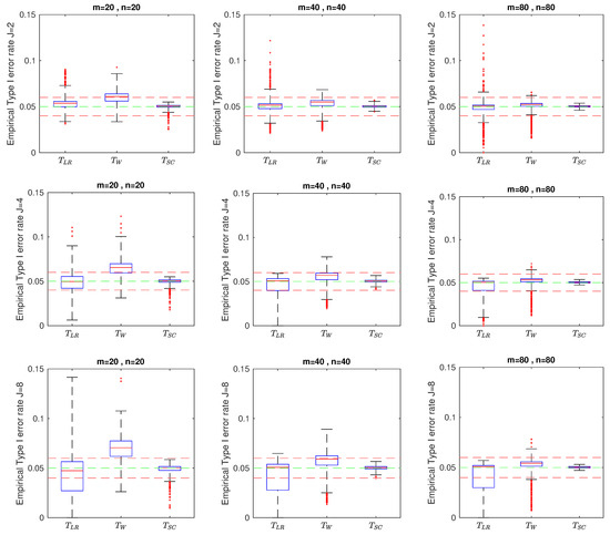
Figure 1. Box plots of empirical sizes when J = 2, 4, 8 and m = n = 20, 40, 80.

As defined by Tang et al. [4], hypothesis testing is classified as liberal if the ratio of the empirical Type I error rate to the nominal Type I error rate is greater than 1.2 (i.e., exceeding 6% for $\alpha$ = 5%, emphasized as bolded numbers in the results). It is considered conservative if this ratio is below 0.8 (i.e., less than 4%, also highlighted in the results) and robust if the ratio falls between 0.8 and 1.2. The results presented in Table 2, Table 3 and Table 4 indicate that the score test $T_{SC}^2$ consistently produces stable Type I error rates across all scenarios. In contrast, the likelihood ratio test is liberal, especially in cases with small sample sizes, while the Wald test exhibits a conservative behavior. Notably, the likelihood ratio test and Wald test tend to be either liberal or conservative with moderate or small sample size (e.g., m = 25 or fewer) and also show similar trends as the correlation coefficient increases. However, when the sample size is sufficiently large (e.g., $m=n=100$ or more, as indicated by the simulation results), both the likelihood ratio test and the Wald test perform comparably to the score test, providing similar results for Type I error rate and power. Consequently, the score test and adjusted chi-square test are preferred for stable control of the Type I error rate.

Next, we assess the power performance of the proposed statistics under similar Type I error parameter settings. The empirical power for $T_{SC}$, $T_L$, and $T_W$ across these settings is shown in Table 5, Table 6 and Table 7. Each table includes footnotes specifying the different settings for each stratum. The simulation results indicate that the score test consistently provides satisfactory power compared to the others. The likelihood ratio test tends to overestimate power due to its empirical level exceeding the nominal level, whereas the Wald test often shows reduced power due to overfitting. As previously mentioned, increasing the sample size results in the power of the three statistics becoming more comparable. The score test is recommended for practical use among the methods evaluated as our conclusion from simulation results.

Table 5. Power performance for J = 2.

			$\mathit{\delta }=(0.8,1.2)$				$\mathit{\delta }=(0.7,1.3)$				$\mathit{\delta }=(0.7,1.2)$
m/n	$\mathit{\rho }$	${\mathit{\pi }}_{\mathit{0}}$	${\mathit{T}}_{\mathit{L}}$	${\mathit{T}}_{\mathit{W}}$	${\mathit{T}}_{\mathit{SC}}$		${\mathit{T}}_{\mathit{L}}$	${\mathit{T}}_{\mathit{W}}$	${\mathit{T}}_{\mathit{SC}}$		${\mathit{T}}_{\mathit{L}}$	${\mathit{T}}_{\mathit{W}}$	${\mathit{T}}_{\mathit{SC}}$
25/25	0.2	0.3	0.1961	0.1483	0.1925		0.3699	0.3268	0.3649		0.2940	0.2452	0.2895
		0.4	0.2695	0.2414	0.2663		0.5239	0.5143	0.5224		0.4106	0.3875	0.4060
	0.5	0.3	0.1797	0.1248	0.1778		0.3395	0.2801	0.3359		0.2624	0.2024	0.2588
		0.4	0.2429	0.2111	0.2410		0.4729	0.4554	0.4708		0.3666	0.3395	0.3650
	0.7	0.3	0.1767	0.1141	0.1717		0.3278	0.2592	0.3233		0.2565	0.1871	0.2520
		0.4	0.2331	0.2006	0.2372		0.4425	0.4358	0.4566		0.3502	0.3224	0.3550
50/50	0.2	0.3	0.3371	0.3182	0.3347		0.6353	0.6271	0.6333		0.5112	0.4972	0.5086
		0.4	0.4824	0.4759	0.4806		0.8170	0.8231	0.8154		0.6924	0.6934	0.6905
	0.5	0.3	0.3060	0.2813	0.3044		0.5829	0.5711	0.5817		0.4635	0.4444	0.4621
		0.4	0.4320	0.4214	0.4308		0.7642	0.7686	0.7633		0.6337	0.6329	0.6327
	0.7	0.3	0.2878	0.2589	0.2868		0.5609	0.5446	0.5599		0.4392	0.4155	0.4375
		0.4	0.4101	0.4021	0.4115		0.7311	0.7423	0.7375		0.6070	0.6025	0.6064
100/100	0.2	0.3	0.5797	0.5755	0.5786		0.8994	0.9015	0.8988		0.8000	0.8002	0.7989
		0.4	0.7622	0.7642	0.7615		0.9796	0.9814	0.9796		0.9294	0.9321	0.9292
	0.5	0.3	0.5307	0.5219	0.5295		0.8582	0.8598	0.8577		0.7430	0.7402	0.7412
		0.4	0.7089	0.7082	0.7087		0.9630	0.9642	0.9626		0.8973	0.8992	0.8971
	0.7	0.3	0.4988	0.4914	0.4983		0.8308	0.8335	0.8306		0.7166	0.7144	0.7161
		0.4	0.6779	0.6772	0.6775		0.9519	0.9540	0.9522		0.8766	0.8778	0.8764
60/50	0.2	0.3	0.3674	0.3491	0.3656		0.6859	0.6812	0.6838		0.5525	0.5429	0.5494
		0.4	0.5188	0.5139	0.5168		0.8561	0.8626	0.8552		0.7344	0.7369	0.7327
	0.5	0.3	0.3238	0.3031	0.3229		0.6196	0.6122	0.6185		0.4978	0.4794	0.4964
		0.4	0.4632	0.4550	0.4624		0.8056	0.8096	0.8050		0.6756	0.6754	0.6744
	0.7	0.3	0.3050	0.2788	0.3044		0.5939	0.5806	0.5925		0.4693	0.4483	0.4683
		0.4	0.4387	0.4285	0.4389		0.7741	0.7792	0.7775		0.6420	0.6414	0.6424

Table 6. Power performance for J = 4.

			$\mathit{\delta }=(0.8,1.2,0.8,1.2)$				$\mathit{\delta }=(0.7,1.3,0.7,1.3)$				$\mathit{\delta }=(0.7,0.8,1.2,1.3)$
m/n	$\mathit{\rho }$	${\mathit{\pi }}_{\mathit{0}}$	${\mathit{T}}_{\mathit{L}}$	${\mathit{T}}_{\mathit{W}}$	${\mathit{T}}_{\mathit{SC}}$		${\mathit{T}}_{\mathit{L}}$	${\mathit{T}}_{\mathit{W}}$	${\mathit{T}}_{\mathit{SC}}$		${\mathit{T}}_{\mathit{L}}$	${\mathit{T}}_{\mathit{W}}$	${\mathit{T}}_{\mathit{SC}}$
25/25	0.2	0.3	0.2338	0.1761	0.2260		0.4669	0.4105	0.4565		0.2940	0.2452	0.2895
		0.4	0.3400	0.3020	0.3326		0.6681	0.6524	0.6653		0.4106	0.3875	0.4060
	0.5	0.3	0.2083	0.1446	0.2027		0.4270	0.3485	0.4202		0.2624	0.2024	0.2588
		0.4	0.3001	0.2501	0.2958		0.6078	0.5795	0.6066		0.3666	0.3395	0.3650
	0.7	0.3	0.2048	0.1307	0.1955		0.4115	0.3165	0.4015		0.2565	0.1871	0.2520
		0.4	0.2768	0.2374	0.2839		0.5597	0.5538	0.5831		0.3502	0.3224	0.3550
50/50	0.2	0.3	0.4256	0.3881	0.4198		0.7922	0.7860	0.7896		0.5112	0.4972	0.5086
		0.4	0.6063	0.5966	0.6028		0.9412	0.9443	0.9394		0.6924	0.6934	0.6905
	0.5	0.3	0.3806	0.3387	0.3765		0.7303	0.7125	0.7279		0.4635	0.4444	0.4621
		0.4	0.5463	0.5282	0.5432		0.9070	0.9095	0.9058		0.6337	0.6329	0.6327
	0.7	0.3	0.3530	0.3064	0.3495		0.7040	0.6816	0.7012		0.4392	0.4155	0.4375
		0.4	0.5126	0.4961	0.5125		0.8797	0.8874	0.8844		0.6070	0.6025	0.6064
100/100	0.2	0.3	0.7243	0.7164	0.7223		0.9812	0.9818	0.9809		0.8000	0.8002	0.7989
		0.4	0.9044	0.9062	0.9034		0.9994	0.9996	0.9994		0.9294	0.9321	0.9292
	0.5	0.3	0.6674	0.6562	0.6663		0.9631	0.9647	0.9629		0.7430	0.7402	0.7412
		0.4	0.8569	0.8573	0.8558		0.9977	0.9982	0.9977		0.8973	0.8992	0.8971
	0.7	0.3	0.6346	0.6165	0.6339		0.9512	0.9512	0.9506		0.7166	0.7144	0.7161
		0.4	0.8300	0.8284	0.8294		0.9957	0.9963	0.9957		0.8766	0.8778	0.8764
60/50	0.2	0.3	0.4637	0.4338	0.4599		0.8378	0.8331	0.8356		0.5525	0.5429	0.5494
		0.4	0.6586	0.6496	0.6559		0.9623	0.9656	0.9616		0.7344	0.7369	0.7327
	0.5	0.3	0.4079	0.3712	0.4053		0.7758	0.7631	0.7739		0.4978	0.4794	0.4964
		0.4	0.5909	0.5768	0.5890		0.9324	0.9334	0.9318		0.6756	0.6754	0.6744
	0.7	0.3	0.3820	0.3416	0.3798		0.7438	0.7268	0.7416		0.4693	0.4483	0.4683
		0.4	0.5550	0.5401	0.5549		0.9098	0.9149	0.9140		0.6420	0.6414	0.6424

Table 7. Power performance for J = 8.

			$\mathit{\delta }=(0.8,1.2,0.8,1.2$				$\mathit{\delta }=(0.7,1.3,0.7,1.3$				$\mathit{\delta }=(0.7,0.8,1.2,1.3$
			$\mathit{0}.\mathit{8},\mathit{1}.\mathit{2},\mathit{0}.\mathit{8},\mathit{1}.\mathit{2})$				$\mathit{0}.\mathit{7},\mathit{1}.\mathit{3},\mathit{0}.\mathit{7},\mathit{1}.\mathit{3})$				$\mathit{0}.\mathit{7},\mathit{0}.\mathit{8},\mathit{1}.\mathit{2},\mathit{1}.\mathit{3})$
m/n	$\mathit{\rho }$	${\mathit{\pi }}_{\mathit{0}}$	${\mathit{T}}_{\mathit{L}}$	${\mathit{T}}_{\mathit{W}}$	${\mathit{T}}_{\mathit{SC}}$		${\mathit{T}}_{\mathit{L}}$	${\mathit{T}}_{\mathit{W}}$	${\mathit{T}}_{\mathit{SC}}$		${\mathit{T}}_{\mathit{L}}$	${\mathit{T}}_{\mathit{W}}$	${\mathit{T}}_{\mathit{SC}}$
25/25	0.2	0.3	0.3019	0.2450	0.2909		0.6193	0.5921	0.6062		0.4722	0.4240	0.4582
		0.4	0.4635	0.4227	0.4532		0.8502	0.8526	0.8502		0.6936	0.6779	0.6888
	0.5	0.3	0.2710	0.1992	0.2626		0.5856	0.5067	0.5763		0.4348	0.3471	0.4220
		0.4	0.4041	0.3556	0.3971		0.7998	0.7807	0.7957		0.6378	0.6011	0.6332
	0.7	0.3	0.2734	0.1808	0.2575		0.5736	0.4760	0.5581		0.4276	0.3196	0.4096
		0.4	0.3683	0.3341	0.3784		0.7347	0.7491	0.7670		0.5763	0.5673	0.6065
50/50	0.2	0.3	0.5932	0.5546	0.5865		0.9428	0.9399	0.9405		0.8306	0.8168	0.8260
		0.4	0.8052	0.7995	0.8017		0.9911	0.9970	0.9910		0.9601	0.9646	0.9595
	0.5	0.3	0.5305	0.4817	0.5260		0.9104	0.8979	0.9083		0.7711	0.7453	0.7679
		0.4	0.7457	0.7347	0.7424		0.9840	0.9913	0.9839		0.9316	0.9351	0.9304
	0.7	0.3	0.4975	0.4415	0.4913		0.8882	0.8715	0.8865		0.7371	0.7026	0.7333
		0.4	0.7090	0.6952	0.7100		0.9737	0.9848	0.9762		0.9105	0.9181	0.9139
100/100	0.2	0.3	0.9040	0.9015	0.9033		0.9997	0.9996	0.9997		0.9934	0.9935	0.9932
		0.4	0.9881	0.9880	0.9879		0.9999	0.9999	0.9999		0.9999	0.9999	0.9999
	0.5	0.3	0.8563	0.8490	0.8548		0.9982	0.9984	0.9982		0.9845	0.9844	0.9845
		0.4	0.9739	0.9742	0.9735		0.9997	0.9999	0.9997		0.9993	0.9996	0.9993
	0.7	0.3	0.8274	0.8188	0.8263		0.9974	0.9974	0.9974		0.9763	0.9754	0.9758
		0.4	0.9668	0.9658	0.9661		0.9997	0.9999	0.9997		0.9986	0.9987	0.9986
60/50	0.2	0.3	0.6426	0.6107	0.6371		0.9645	0.9634	0.9636		0.8768	0.8686	0.8737
		0.4	0.8525	0.8489	0.8502		0.9944	0.9986	0.9944		0.9755	0.9786	0.9749
	0.5	0.3	0.5661	0.5249	0.5618		0.9375	0.9307	0.9361		0.8198	0.8038	0.8172
		0.4	0.7882	0.7764	0.7855		0.9906	0.9943	0.9902		0.9598	0.9614	0.9593
	0.7	0.3	0.5336	0.4885	0.5302		0.9177	0.9070	0.9160		0.7887	0.7628	0.7852
		0.4	0.7511	0.7315	0.7523		0.9878	0.9904	0.9893		0.9407	0.9432	0.9434

4. Application

To address the unilateral and bilateral combined data structure, a double-blinded clinical trial reported by Mandel et al. [21] and Le [20] provides us with the ability to implement our methodology for real-world data. This trial aimed to compare the efficacy of two antibiotics, Cefaclor and Amoxicillin, in treating acute otitis media with effusion (AOM) in children. The study sought to evaluate the safety and effectiveness of Cefaclor compared to Amoxicillin, the standard first-line treatment, in order to identify potentially more effective medications [22]. The trial involved 214 children (293 ears) who received either unilateral or bilateral tympanocentesis before being randomly assigned to one of the treatment groups. After a 14-day treatment course, outcomes were recorded. The unilateral group had binary outcomes (cured or not cured), while the bilateral group was categorized into three outcomes: cured (both ears AOM-free), partially cured (one ear AOM-free), and not cured. Table 8 summarizes the frequency of patients in each outcome category by intervention group at the end of the trial.

Table 8. Number of ears in different age strata of children cured by antibiotics (Treatment arm—Cefaclor vs. Control arm—Amoxicillin).

		Age Group
		<2 yrs			2–5 yrs			≥6 yrs
	Number of AOM-Free Ears	TRT	Control		TRT	Control		TRT	Control
Bilateral	0	8	11		6	3		0	1
	1	2	2		6	1		1	0
	2	8	2		10	5		3	6
Unilateral	0	3	2		24	14		11	11
	1	9	10		7	22		8	7

The parameter estimates shown in Table 9 and Table 10 provide the statistics and corresponding p-values for the three methods. Notably, all p-values are greater than 0.05. Table 9 indicates no evidence to reject the null hypothesis $H_0:{\delta }_1={\delta }_2=\dots ={\delta }_J=\delta$ with $J=3$, suggesting that there is no significant difference in the proportions between Cefaclor and Amoxicillin across the strata.

Table 9. MLEs of risk ratios, correlation coefficient, and risk incidence for each strata.

	Constrained MLEs					Unconstrained MLEs
Age	$\mathit{\delta }$	$\mathit{\rho }$	${\mathit{\pi }}_{\mathit{1}}$	${\mathit{\pi }}_{\mathit{2}}$		$\mathit{\delta }$	$\mathit{\rho }$	${\mathit{\pi }}_{\mathit{1}}$	${\mathit{\pi }}_{\mathit{2}}$
<2 yrs	1.1007	0.7654	0.5022	0.5528		0.7663	0.6756	0.5921	0.4527
2–5 yrs		0.5502	0.4770	0.5250		1.5284	0.5599	0.4011	0.6130
≥6 yrs		0.8111	0.4926	0.5422		1.0489	0.8118	0.5065	0.5312

Table 10. Statistic and p-value for comparing two groups treatment effect.

Method	${\mathit{T}}_{\mathit{LR}}$	${\mathit{T}}_{\mathit{W}}$	${\mathit{T}}_{\mathit{SC}}$
statistic	4.5624	4.6593	4.8774
p-value	0.1022	0.0973	0.0873

5. Conclusions

In this article, we developed three test procedures to assess homogeneity in combined unilateral and bilateral samples within stratified two-group clinical trial data. For the estimation of unrestricted and restricted MLEs, we proposed relatively efficient iteration solutions by treating relative risks as common to decrease the estimator dimension.

Simulation results demonstrate that the score test performs robustly, maintaining a satisfactory Type I error rate and power across various parameter settings, including different group sizes and numbers of strata. In contrast, the likelihood ratio test tends to produce inflated results when sample sizes are small, while the Wald test is conservative and prone to overfitting with small sample sizes. However, as the number of strata increases and the relative risk becomes larger, the Wald test’s performance also becomes inflated. When the sample size is large, especially when it exceeds 100, the results of the three tests converge closely to the true values. Therefore, the score test is generally preferred for assessing homogeneity in combined sample designs. Simulation results furthermore indicated that a combined data structure incorporating unilateral and bilateral data at once could gain more power than bilateral data only [19].

This study utilizes a statistical approach grounded in Donner’s parametric model, which calculates the rate by aggregating outcomes across groups, treating paired organs and bilateral results as indistinguishable. Given the inflated or conservative Type I error rates observed in the likelihood ratio and Wald tests, future research may explore the development of an exact test tailored to small sample size settings. It is important to note that Donner’s model assumes a common intra-class correlation for bilateral outcomes, which may present challenges if significant differences in correlation exist between the paired organs of different individuals or across different groups in clinical trials. In other words, we should initially validate the correlation in conjunction with our model-based method presentation. In addition, there is necessity to adjust for confounding effect when we involves in strata. Furthermore, some research examines the difference between the paired organs such eyes can be dominant and non-dominant [23] while researchers usually do not collect (or it is hard to collect) the handedness of the individuals [1]. We could consider if those data are available in a real-world example. Considering the assumptions discussed above, we plan to explore these topics in future work to support our methods using a more stable foundation.

In addition to risk ratio exploration, Zhang and Ma [24] investigated homogeneity testing on the risk difference between stratified bilateral and unilateral combined data. She proposed that the score test is a worthwhile hypothesis testing with well-performed power and a robust Type I error rate, which can be evidence supporting that our model-based method on risk ratio holds more comprehensive conclusions.

Appendix A.1. Fisher Information Matrix for Given δ

Under the null hypothesis, ${\pi }_{1j}$ and ${\rho }_j$ can be obtained by the Fisher scoring algorithm. The Fisher information matrix for jth stratum is written as follows:

$${\mathit{I}}_1^{\left(j\right)}=\left[\begin{array}{cc}{I}_{11}^{1j}& I_{12}^{1j}\\ I_{12}^{1j}& I_{22}^{1j}\end{array}\right]=\left[\begin{array}{cc}{m}_{+1j}{A}_1+m_{+2j}{\delta }^2{A}_2+A_3& m_{+1j}{B}_1+m_{+2j}\delta B_2\\ m_{+1j}{B}_1+m_{+2j}\delta B_2& m_{+1j}{C}_1+m_{+2j}{C}_2\end{array}\right],$$

where

$$\begin{array}{cc}\hfill A_1& ={\displaystyle \frac{(2-2{\rho }_j)(2{{\pi }_{1j}}^2-2{\pi }_{1j}+1)}{{\pi }_{1j}(1-{\pi }_{1j})}}\hfill \\ \hfill & +{\displaystyle \frac{(2{{\pi }_{1j}}^2+1){(1-{\rho }_j)}^2-2{\pi }_{1j}(1-{\rho }_j)(2-{\rho }_j)+1}{{(1-{\pi }_{1j})}^2(1-{\rho }_j)+{\rho }_j(1-{\pi }_{1j})}}\hfill \\ \hfill & +{\displaystyle \frac{2{{\pi }_{1j}}^2{(1-{\rho }_j)}^2+{\rho }_j^2+2{\pi }_{1j}{\rho }_j(1-{\rho }_j)}{{{\pi }_{1j}}^2(1-{\rho }_j)+{\pi }_{1j}{\rho }_j}},\hfill \end{array}$$

$$\begin{array}{cc}\hfill A_2& ={\displaystyle \frac{{\rho }_j^2+2{\delta }^2{{\pi }_{1j}}^2{(1-{\rho }_j)}^2+2\delta {\pi }_{1j}{\rho }_j(1-{\rho }_j)}{\delta {\pi }_{1j}{\rho }_j-{\delta }^2{{\pi }_{1j}}^2({\rho }_j-1)}}\hfill \\ \hfill & +{\displaystyle \frac{(2{\delta }^2{{\pi }_{1j}}^2+1){(1-{\rho }_j)}^2-2\delta {\pi }_{1j}(1-{\rho }_j)(2-{\rho }_j)+1}{{(1-\delta {\pi }_{1j})}^2(1-{\rho }_j)+{\rho }_j(1-\delta {\pi }_{1j})}}\hfill \\ \hfill & +{\displaystyle \frac{(2-2{\rho }_j)(2{\delta }^2{{\pi }_{1j}}^2-2\delta {\pi }_{1j}+1)}{\delta {\pi }_{1j}(1-\delta {\pi }_{1j})}},\hfill \end{array}$$

$$A_3=n_{+1j}{\displaystyle \frac{1}{{\pi }_{1j}(1-{\pi }_{1j})}}+n_{+2j}{\displaystyle \frac{\delta }{{\pi }_{1j}(1-\delta {\pi }_{1j})}},$$

$$B_1={\displaystyle \frac{1-{\pi }_{1j}}{{\rho }_j+(1-{\pi }_{1j})(1-{\rho }_j)}}+{\displaystyle \frac{{\pi }_{1j}}{{\rho }_j+{\pi }_{1j}(1-{\rho }_j)}},$$

$$B_2={\displaystyle \frac{1-\delta {\pi }_{1j}}{{\rho }_j+(1-\delta {\pi }_{1j})(1-{\rho }_j)}}+{\displaystyle \frac{\delta {\pi }_{1j}}{{\rho }_j+\delta {\pi }_{1j}(1-{\rho }_j)}},$$

$$C_1={\displaystyle \frac{2{\pi }_{1j}(1-{\pi }_{1j})}{1-{\rho }_j}}+{\displaystyle \frac{{{\pi }_{1j}}^2(1-{\pi }_{1j})}{{\rho }_j+(1-{\pi }_{1j})(1-{\rho }_j)}}+{\displaystyle \frac{{\pi }_{1j}{(1-{\pi }_{1j})}^2}{{\rho }_j+{\pi }_{1j}(1-{\rho }_j)}},$$

$$C_2={\displaystyle \frac{2\delta {\pi }_{1j}(1-\delta {\pi }_{1j})}{1-{\rho }_j}}+{\displaystyle \frac{{{\delta }^2{\pi }_{1j}}^2(1-\delta {\pi }_{1j})}{{\rho }_j+(1-\delta {\pi }_{1j})(1-{\rho }_j)}}+{\displaystyle \frac{\delta {\pi }_{1j}{(1-\delta {\pi }_{1j})}^2}{{\rho }_j+\delta {\pi }_{1j}(1-{\rho }_j)}}.$$

Appendix A.2. Fisher Information Matrix for the Wald Test and Score Test

The Fisher information matrix $\mathit{I}$ is a $3J\times 3J$ block diagonal matrix.

$$\mathit{I}=\left[\begin{array}{cccc}{\mathit{I}}_1& \mathit{0}& \dots & 0\\ \mathit{0}& {\mathit{I}}_2& \dots & 0\\ ⋮& & \ddots & ⋮\\ \mathit{0}& \dots & \dots & {\mathit{I}}_J,\end{array}\right]$$

with the diagonal elements

$${\mathit{I}}_j=\left[\begin{array}{ccc}{I}_{11}^j& I_{12}^j& I_{13}^j\\ I_{12}^j& I_{22}^j& I_{23}^j\\ I_{13}^j& I_{23}^j& I_{33}^j,\end{array}\right]$$

where

$$\begin{array}{cc}\hfill I_{11}^j& =m_{+2j}{\pi }_{1j}^2[{\displaystyle \frac{(2-2{\rho }_j)(2{{\pi }_{1j}}^2-2{\pi }_{1j}+1)}{{\pi }_{1j}(1-{\pi }_{1j})}}\hfill \\ \hfill & +{\displaystyle \frac{(2{{\pi }_{1j}}^2+1){(1-{\rho }_j)}^2-2{\pi }_{1j}(1-{\rho }_j)(2-{\rho }_j)+1}{{(1-{\pi }_{1j})}^2(1-{\rho }_j)+{\rho }_j(1-{\pi }_{1j})}}\hfill \\ \hfill & +{\displaystyle \frac{2{{\pi }_{1j}}^2{(1-{\rho }_j)}^2+{\rho }_j^2+2{\pi }_{1j}{\rho }_j(1-{\rho }_j)}{{{\pi }_{1j}}^2(1-{\rho }_j)+{\pi }_{1j}{\rho }_j}}]\hfill \\ \hfill & +n_{+2j}{\pi }_{1j}^2{\displaystyle \frac{1}{{\delta }_j{\pi }_{1j}(1-{\delta }_j{\pi }_{1j})}},\hfill \end{array}$$

$$I_{12}^j={\displaystyle \frac{{\delta }_j}{{\pi }_{1j}}}{I}_{w11}^j,$$

$$I_{13}^j=m_{+2j}{\pi }_{1j}\left[{\displaystyle \frac{1-\delta {\pi }_{1j}}{{\rho }_j+(1-\delta {\pi }_{1j})(1-{\rho }_j)}}+{\displaystyle \frac{\delta {\pi }_{1j}}{{\rho }_j+\delta {\pi }_{1j}(1-{\rho }_j)}}\right],$$

$$\begin{array}{cc}\hfill I_{22}^j& =m_{+1j}[{\displaystyle \frac{(2-2{\rho }_j)(2{{\pi }_{1j}}^2-2{\pi }_{1j}+1)}{{\pi }_{1j}(1-{\pi }_{1j})}}\hfill \\ \hfill & +{\displaystyle \frac{(2{{\pi }_{1j}}^2+1){(1-{\rho }_j)}^2-2{\pi }_{1j}(1-{\rho }_j)(2-{\rho }_j)+1}{{(1-{\pi }_{1j})}^2(1-{\rho }_j)+{\rho }_j(1-{\pi }_{1j})}}\hfill \\ \hfill & +{\displaystyle \frac{2{{\pi }_{1j}}^2{(1-{\rho }_j)}^2+{\rho }_j^2+2{\pi }_{1j}{\rho }_j(1-{\rho }_j)}{{{\pi }_{1j}}^2(1-{\rho }_j)+{\pi }_{1j}{\rho }_j}}]\hfill \\ \hfill & +m_{+2j}{\delta }^2[{\displaystyle \frac{{\rho }_j^2+2{\delta }^2{{\pi }_{1j}}^2{(1-{\rho }_j)}^2+2\delta {\pi }_{1j}{\rho }_j(1-{\rho }_j)}{\delta {\pi }_{1j}{\rho }_j-{\delta }^2{{\pi }_{1j}}^2({\rho }_j-1)}}\hfill \\ \hfill & +{\displaystyle \frac{(2{\delta }^2{{\pi }_{1j}}^2+1){(1-{\rho }_j)}^2-2\delta {\pi }_{1j}(1-{\rho }_j)(2-{\rho }_j)+1}{{(1-\delta {\pi }_{1j})}^2(1-{\rho }_j)+{\rho }_j(1-\delta {\pi }_{1j})}}\hfill \\ \hfill & +{\displaystyle \frac{(2-2{\rho }_j)(2{\delta }^2{{\pi }_{1j}}^2-2\delta {\pi }_{1j}+1)}{\delta {\pi }_{1j}(1-\delta {\pi }_{1j})}}]\hfill \\ \hfill & +n_{+1j}{\displaystyle \frac{1}{{\pi }_{1j}(1-{\pi }_{1j})}}+n_{+2j}{\displaystyle \frac{\delta }{{\pi }_{1j}(1-\delta {\pi }_{1j})}},\hfill \end{array}$$

$$\begin{array}{cc}\hfill I_{23}^j& =m_{+1j}\left[{\displaystyle \frac{1-{\pi }_{1j}}{{\rho }_j+(1-{\pi }_{1j})(1-{\rho }_j)}}+{\displaystyle \frac{{\pi }_{1j}}{{\rho }_j+{\pi }_{1j}(1-{\rho }_j)}}\right]\hfill \\ \hfill & +m_{+2j}\delta \left[{\displaystyle \frac{1-\delta {\pi }_{1j}}{{\rho }_j+(1-\delta {\pi }_{1j})(1-{\rho }_j)}}+{\displaystyle \frac{\delta {\pi }_{1j}}{{\rho }_j+\delta {\pi }_{1j}(1-{\rho }_j)}}\right],\hfill \end{array}$$

$$\begin{array}{cc}\hfill I_{33}^j& =m_{+1j}\left[{\displaystyle \frac{2{\pi }_{1j}(1-{\pi }_{1j})}{1-{\rho }_j}}+{\displaystyle \frac{{{\pi }_{1j}}^2(1-{\pi }_{1j})}{{\rho }_j+(1-{\pi }_{1j})(1-{\rho }_j)}}+{\displaystyle \frac{{\pi }_{1j}{(1-{\pi }_{1j})}^2}{{\rho }_j+{\pi }_{1j}(1-{\rho }_j)}}\right]\hfill \\ \hfill & +m_{+2j}\left[{\displaystyle \frac{2\delta {\pi }_{1j}(1-\delta {\pi }_{1j})}{1-{\rho }_j}}+{\displaystyle \frac{{{\delta }^2{\pi }_{1j}}^2(1-\delta {\pi }_{1j})}{{\rho }_j+(1-\delta {\pi }_{1j})(1-{\rho }_j)}}+{\displaystyle \frac{\delta {\pi }_{1j}{(1-\delta {\pi }_{1j})}^2}{{\rho }_j+\delta {\pi }_{1j}(1-{\rho }_j)}}\right].\hfill \end{array}$$

References

- Fan, Q.; Teo, Y.Y.; Saw, S.M. Application of Advanced Statistics in Ophthalmology. Investig. Ophthalmol. Vis. Sci. 2011, 52, 6059–6065. [Google Scholar] [CrossRef]
- Burton, P.; Gurrin, L.; Sly, P. Extending the simple linear regression model to account for correlated responses: An introduction to generalized estimating equations and multi-level mixed modelling. Stat. Med. 1998, 17, 1261–1291. [Google Scholar] [CrossRef]
- Murdoch, I.E.; Morris, S.S.; Cousens, S.N. People and eyes: Statistical approaches in ophthalmology. Br. J. Ophthalmol. 1998, 82, 971–973. [Google Scholar] [CrossRef]
- Tang, N.S.; Tang, M.L.; Qiu, S.F. Testing the equality of proportions for correlated otolaryngologic data. Comput. Stat. Data Anal. 2008, 52, 2719–3729. [Google Scholar] [CrossRef]
- Ma, C.X.; Shan, G.; Liu, S. Homogeneity test for binary correlated data. PLoS ONE 2015, 10, e0124337. [Google Scholar] [CrossRef]
- Shan, G.; Ma, C. Exact methods for testing the equality of proportions for binary clustered data from otolaryngologic studies. Stat. Biopharm. Res. 2014, 6, 115–122. [Google Scholar] [CrossRef]
- Liu, X.; Shan, G.; Tian, L.; Ma, C.X. Exact methods for testing homogeneity of proportions for multiple groups of paired binary data. Commun. Stat.—Simulat. Comput. 2017, 46, 6074–6082. [Google Scholar] [CrossRef]
- Dallal, G.E. Paired Bernoulli Trials. Biometrics 1988, 44, 253–257. [Google Scholar] [CrossRef]
- Donner, A. Statistical methods in ophthalmology: An adjusted chi-square approach. Biometrics 1989, 45, 605–611. [Google Scholar] [CrossRef]
- Thompson, J.R. The chi-square test for data collected on eyes. Br. J. Ophthalmol. 1993, 77, 115–117. [Google Scholar] [CrossRef]
- Donner, A.; Klar, N. Methods for comparing event rates in intervention studies when the unit of allocation is a cluster. Am. J. Epidemiol. 1994, 140, 279–289. [Google Scholar] [CrossRef] [PubMed]
- Jung, S.H.; Ahn, C.D.A. A study of an adjusted χ2 statistic as applied to observational studies involving clustered binary data. Stat. Med. 2001, 20, 2149–2161. [Google Scholar] [CrossRef] [PubMed]
- Tang, N.S.; Qiu, S.F.; Tang, M.L.; Pei, Y.B. Asymptotic confidence interval construction for proportion difference in medical studies with bilateral data. Stat. Methods Med. Res. 2011, 20, 233–259. [Google Scholar] [CrossRef]
- Pei, Y.B.; Tang, M.L.; Guo, J.H. Testing the equality of two proportions for combined unilateral and bilateral data. Commun. Stat.-Comput. 2008, 37, 1515–1529. [Google Scholar] [CrossRef]
- Ma, C.X.; Liu, S. Testing equality of proportions for correlated binary data in ophthalmologic studies. J. Biopharm. Stat. 2017, 27, 611–619. [Google Scholar] [CrossRef]
- Lui, K.J.; Kelly, C. Tests for homogeneity of the risk ratio in a series of 2 × 2 tables. Stat. Med. 2000, 19, 2919–2932. [Google Scholar] [CrossRef]
- Li, H.Q.; Tang, N.S. Homogeneity test of rate ratios in stratified matched-pair studies. Biom. J. 2011, 53, 614–627. [Google Scholar] [CrossRef]
- Tang, N.S.; Qiu, S.F. Homogeneity test, sample size determination and interval construction of difference of two proportions in stratified bilateral-sample designs. J. Stat. Plan. Inference 2012, 142, 1243–1251. [Google Scholar] [CrossRef]
- Pei, Y.; Tian, G.L.; Tang, M.L. Testing homogeneity of proportion ratios for stratified correlated bilateral data in two-arm randomized clinical trials. Stat. Med. 2014, 33, 4370–4386. [Google Scholar] [CrossRef]
- Le, C.T. Testing for Linear Trends in Proportions Using Correlated Otolaryngology or ophthalmology Data. Biometrics 1988, 44, 299–303. [Google Scholar] [CrossRef]
- Mandel, E.M.; Bluestone, C.D.; Rockette, H.E.; Blatter, M.M.; Reisinger, K.S.; Wucher, F.P.; Harper, J. Duration of effusion after antibiotic treatment for acute otitis media: Comparison of cefaclor and amoxicillin. Pediatr. Infect. Dis. 1982, 1, 310–316. [Google Scholar] [CrossRef]
- McLinn, S.E. Cefaclor in treatment of otitis media and pharyngitis in children. Am. J. Dis. Child. 1980, 134, 560–563. [Google Scholar] [CrossRef] [PubMed]
- Linke, S.J.; Druchkiv, V.; Steinberg, J.; Richard, G.; Katz, T. Eye laterality: A comprehensive analysis in refractive surgery candidates. Acta Ophthalmol. 2013, 91, e363–e368. [Google Scholar] [CrossRef] [PubMed]
- Zhang, X.; Ma, C. Testing the Homogeneity of Differences between Two Proportions for Stratified Bilateral and Unilateral Data across Strata. Mathematics 2023, 11, 4156. [Google Scholar] [CrossRef]
Disclaimer/Publisher’s Note: The statements, opinions and data contained in all publications are solely those of the individual author(s) and contributor(s) and not of MDPI and/or the editor(s). MDPI and/or the editor(s) disclaim responsibility for any injury to people or property resulting from any ideas, methods, instructions or products referred to in the content. |
© 2024 by the authors. Licensee MDPI, Basel, Switzerland. This article is an open access article distributed under the terms and conditions of the Creative Commons Attribution (CC BY) license (https://creativecommons.org/licenses/by/4.0/).