Abstract
This paper explores the numerical intergator of ODE based on combination of Appelroth’s quadratization of dynamical systems with polynomial right-hand sides and Kahan’s discretization method. Utilizing Appelroth’s technique, we reduce any system of ordinary differential equations with a polynomial right-hand side to a quadratic form, enabling the application of Kahan’s method. In this way, we get a difference scheme defining the one-to-one correspondence between the initial and final positions of the system (Cremona map). It provides important information about the Kahan method for differential equations with a quadratic right-hand side, because we obtain dynamical systems with a quadratic right-hand side that have movable branch points. We analyze algebraic properties of solutions obtained through this approach, showing that (1) the Kahan scheme describes the branch points as poles, significantly deviating from the behavior of the exact solution of the problem near these points, and (2) it disrupts algebraic invariant variety, in particular integral relations describing the relationship between old and Appelroth’s variables. This study advances numerical methods, emphasizing the possibility of designing difference schemes whose algebraic properties differ significantly from those of the initial dynamical system.
Keywords:
finite difference method; dynamical systems; computer algebra; birational map; Cremona transformation MSC:
37M15; 14E07; 34A25; 65L12
1. Introduction
At the beginning of the 20th century, G.G. Appelroth [1] noted that any system of ordinary differential equations with a polynomial right-hand side can be reduced to a system of differential equations with a quadratic right-hand side, i.e., the original system can be quardaticized by introducing additional variables. This procedure was introduced recently in the computer algebra field [2,3,4].
In the 2010s, among the difference schemes that inherit some properties of the original differential equations, difference schemes that define birational transformations between layers in time were singled out. Such schemes can be constructed for any system of differential equations with a quadratic right-hand side using a method that some authors associate with the name of W. Kahan [5,6,7], while others associate it with Hirota and Kimura [8,9,10]. We came to this scheme in [11,12] in the way of generalizing the idea of Painlevé about the integration of differential equations in classical transcendental functions [13,14]. Computer experiments presented in these works allow us to hypothesize that (1) the Kahan scheme always inherits algebraic integrals of motion [12] [n. 2] and (2) the solution found by the Kahan scheme imitates the moving singularities of the ODE system [12] [n. 6].
Appelroth’s quadratization allows one to apply Kahan’s method to any dynamical system with a polynomial right-hand side. Continuing our research about difference schemes that define birational maps [12], we consider in this paper the properties of approximate solutions obtained by combining Appelroth’s quadratization and Kahan’s discretization. The simplest computer experiments with quadratized systems showed that both hypotheses expressed above are not true.
2. Kahan Discretization
Newton’s equations define a one-to-one correspondence between the initial and final positions of a dynamical system. Difference schemes approximating Newton’s equations define a correspondence between the initial and final positions of the system, which is described by algebraic equations. Such a correspondence will be one-to-one if and only if it is birational [15].
Any dynamical system can be described as follows:
or, in short:
with a quadratic right-hand side can be approximated by a difference scheme that specifies a birational correspondence between the positions of the system at time t and the position at . Indeed, if we agree to denote the first position simply as and the second as , then this scheme can be written as:
where is obtained from the expression by replacing the monomial with , and the monomial —with . Of course, it is more convenient to use a replacement symmetric with respect to the initial and final values: the monomial changes to , the monomial —to , and the monomial —by . For example, we propose to approximate the Riccati equation:
by the scheme:
This symmetric scheme, like the midpoint scheme and the trapezoidal scheme, obviously has a second order of approximation [16]. But something else is important for us now: the system (2) is linear both with respect to and with respect to . Therefore, can be expressed as a rational function of and, conversely, as a rational function of . Thus, the scheme (2) defines a birational correspondence between points and of an n-dimensional space over the field .
The method of approximating a dynamical system (1) with a quadratic right-hand side described above came into use in the middle of the last century in the field of solitonics [17]. Following a report presented by William Kahan in 1993, this difference scheme was applied to the Volterra–Lotka system [5], to the quadratic Hamiltonian system [6,7], and to the equations of motion of a gyroscope for the two classical cases of Euler–Poinsot [8,10,12,18] and Lagrange–Euler [9]. The fact that Kahan’s difference scheme defines a birational correspondence was first noted in [10].
The focus of these studies was the inheritance of algebraic integrals of motion of the original dynamical system by the Kahan difference scheme. For Hamiltonian systems, explicit expressions for the symplectic structure and the modified Hamiltonian, which are exactly preserved in the Kahan scheme, were obtained in [6]. For the gyroscope, modified expressions for quadratic integrals were given in [8,9], the method for obtaining them was restored in [18]; in our opinion, it is a difference analogue of the Lagutinsky method [12]. These examples allow us to hypothesize that the Kahan scheme always inherits algebraic integrals of motion in sense of the definition given in [12] [n. 2].
If the solution of a differential equation has a moving pole [19], then the solution found by the Kahan scheme imitates it: the plot of the approximate solution clearly shows how the approximate solution goes to infinity, but also returns without noticeable accumulation of error [12] [n. 6]. Computer experiments allow us to express a second hypothesis: the solution found by the Kahan scheme imitates the moving singularities of the ODE system.
For this reason, it is natural to consider the points of the approximate solution as points of the projective space, which is quite consistent with the tradition of considering birational transformations of n-dimensional space as transformations of the projective space [15]. In this case, a birational transformation of n-dimensional space is called the Cremona transformation. Therefore, we can say that the scheme (2) defines Cremona transformation between the new and old positions of the dynamical system (1).
Most of the studied systems can be classified as elliptic oscillators, i.e., dynamical systems for which integral curves are elliptic curves. In this case, as shown in [12], the discrete theory completely repeats the continuous theory: (i) the points of the approximate solution lie on some elliptic curve, which at turns into an integral curve, (ii) the difference scheme allows representation using quadrature, and (iii) the approximate solution can be represented using an elliptic function of the discrete argument. This allows constructing a theory of elliptic functions based on the Cremona transformation (Hermite hypothesis) [12].
Apart stands the Volterra–Lotka system, the integral curves of which are transcendental. Computer experiments with the Kahan scheme show that the points of the approximate solution lie on some transcendental curves, the invariant curves of the corresponding Cremona transformation [12]. Transcendental invariant curves of Cremona transformations were probably first described in [20].
Kahan’s method can be easily transferred to the case of dynamical systems with a polynomial right-hand side. The point is that a dynamical system system with a polynomial right-hand side can always be lifted to a quadratic system by introducing additional variables.
3. Quadratization of Dynamical Systems with a Polynomial Right-Hand Side
Quadratization is a mathematical technique that transforms a system of ordinary differential equations with polynomial right-hand sides into a system with quadratic right-hand sides. This transformation is crucial for the application of numerical methods, particularly finite difference methods, which can be more effectively implemented on quadratic systems. This procedure, first indicated by G.G. Appelroth [1], is called quadratization of a system of differential equations in computer algebra [2,3,4].
In the original work of G.G. Appelroth [1], quadratization is described in projective coordinates. We will describe their method in more familiar affine coordinates.
Let the right-hand sides of the differential equations of system (1) be polynomials in and let m be the largest degree of the polynomials . Denote by M the set of all monomials:
whose degree, shown as follows:
is strictly less than m but greater than 1. We enumerate the monomials in this set in any order and denote them as . Then, any polynomial whose degree does not exceed m is a linear combination of and all their possible products of the form . Therefore, the system (1) can be rewritten as:
where are constants.
Let . Then:
or
When multiplying by , we get a monomial from M or . Therefore, the left-hand side of (4) is a linear combination of products having the form , , and :
By adding the system (1), written in the form (3), to the system (5), we arrive at a system of differential equations with a linear or quadratic right-hand side, in which the number of sought functions coincides with the number of equations.
Thus:
Quadratization of a given ODE system with a polynomial right-hand side is performed in two steps.
- Introduction of additional variables: to achieve quadratization, additional variables are introduced. In the original approach of Appelroth, all monomials whose degrees are strictly less than the largest degree of the polynomials of right-hand site of ODEs are chosen as these variables. Modern quadratization algorithms like Qbee by A. Bychkov [21] tend to reduce the number of variables entered.
- Reformulation of the system: the new extended ODE system consists of two subsystems. The first of them is obtained from the original by expressing the right-hand sides of ODE as quadratic polynomials with respect to old and new variables. The second is obtained by differentiating algebraic equations between new and old variables.
Let us illustrate Appelroth’s method with a simple example.
Example 1.
The degree of is 2, and the degree of is 3, so . The set M is formed by monomials whose degree lies between 1 and 3 strictly, that is, monomials of the second order:
We rewrite the original system in the form (3), that is:
Next, we construct the system (5):
As a result, we have:
In this case:
that is:
Furthermore:
or
Therefore, the manifold:
is integral. Finally:
or
Therefore, the manifold:
is integral.
The number of additional variables introduced in Appelroth’s quadratization can be excessive. An algorithm has now been developed that can significantly reduce this number in some cases [3]. Currently, there are several implementations of quadratization: Qbee by A. Bychkov [21] and BioCham [2]. Qbee is below used for quadratization in complex cases. All numerical calculations were made in our system FDM for Sage [22].
4. Branch Points in Kahan’s Discretization
In the scalar case, the analytic properties of solutions of the differential equation, shown as follows:
with a quadratic right-hand side, i.e., the Riccati equation, are well studied [23]. First, the general solution of the Riccati equation defines a birational correspondence between the initial and final values. The approximation of the Riccati equation according to the Kahan scheme inherits this property. Second, the Riccati equation possesses the Painlevé property, i.e., it has only poles as moving singular points. This property is also inherited under the Kahan discretization: the approximate solution goes to infinity and returns back without noticeable accumulation of error ([12], n. 6). Moreover, Kahan’s scheme correctly describes the behavior of the solution after the moving singular points, the corresponding estimates were given in [11].
However, if the right-hand side of the scalar Equation (6) is a polynomial whose degree is strictly greater than 2, then its general solution no longer specifies a one-to-one correspondence between the initial and final values. Nevertheless, quadratization allows a replacement with a system having a quadratic right-hand side, and the Kahan scheme allows approximating this system in such a way that the transition from one time layer to another is described by a birational transformation. Thus, the approximate solution acquires an algebraic property that is not inherent in the solution of the original differential equation.
Moreover, if the degree of f is higher than 2, then Equation (6) does not have also the Painlevé property: among its moving points there are critical (algebraic) points [23]. However, the quadratization allows replacing the original equations by a system with a quadratic right-hand side. Will Kahan’s scheme allow imitating algebraic singularities?
To answer this question, let us consider the initial value problem:
the exact solution of which, shown as follows:
has a branch point at . Appelroth’s squaring requires introducing one new variable , which yields a quadraticized system:
and the integral manifold:
on which it is equivalent to the original differential equation.
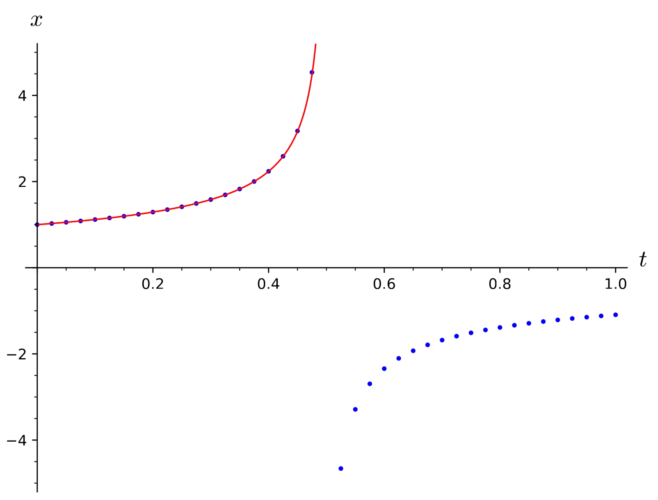
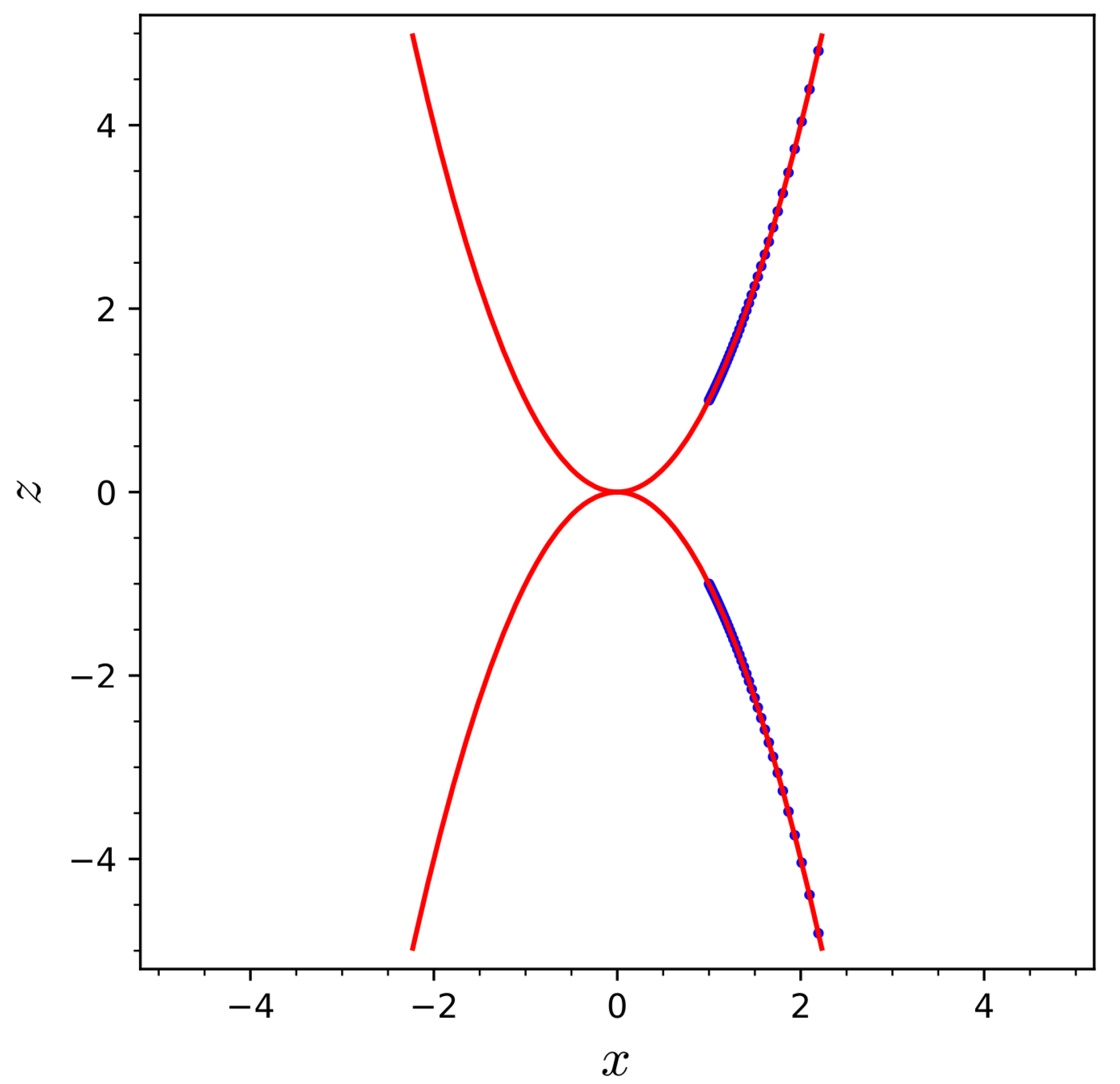
For this system with a quadratic right-hand side, we construct the Kahan scheme and find a solution to the problem (7) using it. In Figure 1, it is evident that the points of the approximate solution lie on the integral curve of the problem (7) only up to the branch point . After this point, the integral curve (8) becomes imaginary, and the approximate solution remains real. Moreover, the points of the approximate solution behave at the branch point as if it were a pole of odd order: they go upward to infinity and return from below.
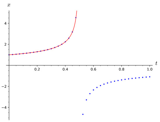
Figure 1.
Solution of the initial value problem (7) obtained using the Kahan scheme (dots) and the exact solution (solid line).
Thus, after quadratization, the Kahan scheme describes the branch points as poles, significantly deviating from the behavior of the exact solution of the problem. We can say that after quadratization, the Kahan scheme imposes on the approximate solution properties typical of the Riccati equation, turning algebraic singularities into poles.
In fact, Appelroth’s theorem is the cause of a number of difficulties both in the analytical theory of differential equations and in the theory of Kahan’s schemes. First, when quadraticizing Equation (6), we easily obtain a system with a quadratic right-hand side that does not have the Painlevé property. It follows that among systems with a quadratic right-hand side, only the chosen ones have this property, which was an unpleasant surprise for analysts of the second half of the 19th century, who hoped to integrate such equations, including the equations of gyroscope motion, in single-valued functions of time [19]. Second, when discretizing systems with a quadratic right-hand side using Kahan’s method, we can obtain poles where the exact solution has an algebraic singularity. Thus, Kahan’s scheme does not imitate the analytical properties of the solution of a system of differential equations, but imposes the Painlevé property on this system.
5. Integral Relations Describing the Relationship between New and Old Variables
No less interesting conclusions can be made regarding the conservation of algebraic integrals. Recall that during quadratization a whole series of integral relations arise, describing the connection between the original variables and additional variables.
For example, for the differential Equation (7) there is one such connection:
From the point of view of the theory of integral manifolds, the polynomial is the Darboux integral of the system (9) in the sense that:
However, in this case, we can say more simply that this integral manifold is the equilevel line of the algebraic integral of the system (9), i.e.
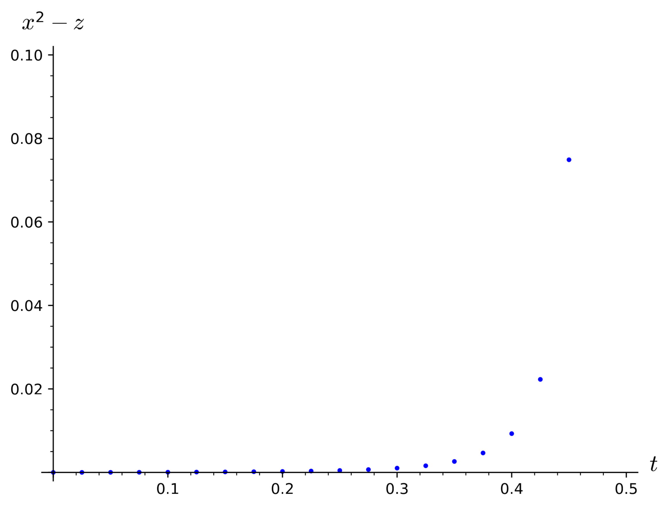
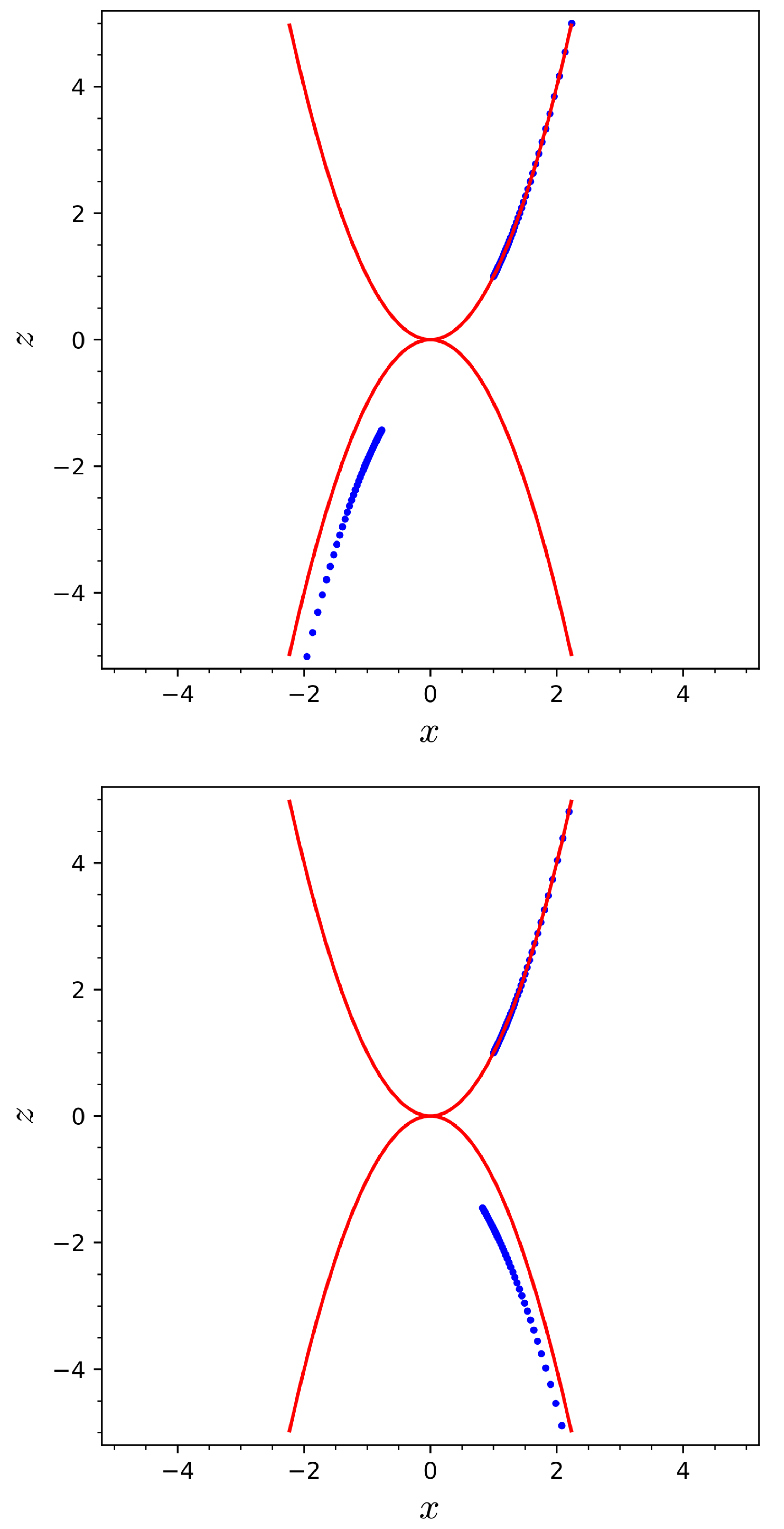
On the exact solution of the system (9) with the initial conditions , the polynomial must be equal to zero. Figure 2 shows the dependence of u on the approximate solution of this problem, found using the Kahan scheme. It is clearly seen that as the branching point is approached, the value of u becomes larger and larger. At the branching point itself, this quantity takes on a huge value of the order of . In Figure 3 and Figure 4, one can see that the points of the approximate solution fit perfectly the parabola up to the moment , and then pass to the curve , which is also an equilevel line of the integral of the system (9), but with a different value of the constant. The position of the points on the first parabola stabilizes when tends to zero (as it should be by virtue of the well-known convergence theorem [16]), and the position of the points on the second parabola, on the contrary, significantly depends on the choice of step.
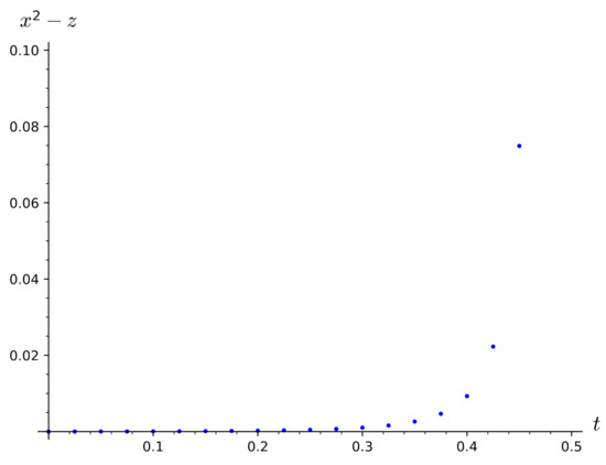
Figure 2.
The value of the polynomial for the solution of the initial value problem (7), obtained using the Kahan scheme.
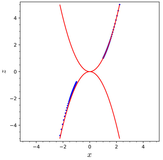
Figure 3.
Solution of the initial value problem (7) at , obtained using the Kahan scheme, in the plane (points) with and the parabolas and (solid line).
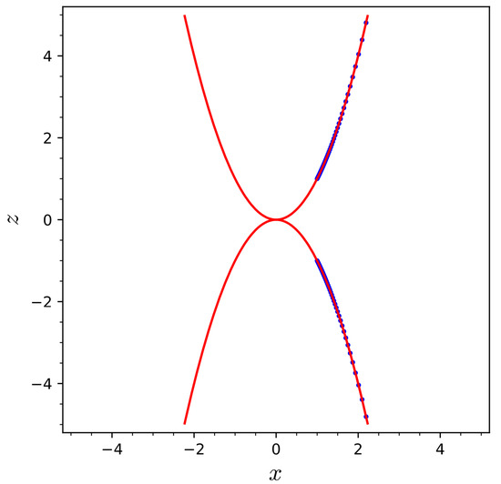
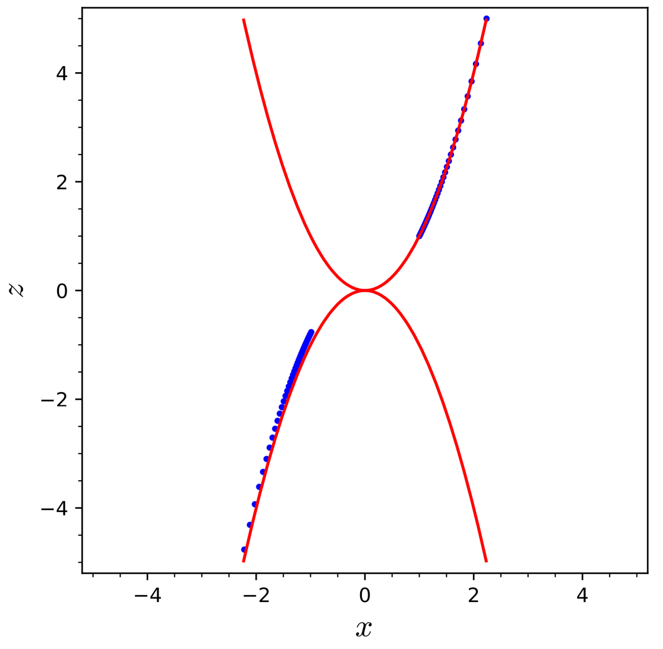
Figure 4.
Solution of the initial value problem (7) at , obtained using the Kahan scheme, in the plane (points) and the parabolas and (solid line).
This example shows that the integral relations describing the relationship between new and old variables are violated, and this violation becomes especially noticeable at branching points.
It is also known that quadratization can destroy some stability properties of the original system, so one could attribute the observed instability to this phenomenon as well. Moreover, [4] proposed to use the non-uniqueness of quadratization to mitigate this issue. Thus, we can try to use the system:
where is real constant. The new term “punishes” the system for leaving the invariant manifold . The expression is a Darboux integral for both the system (9) and the system (11) and on the invariant manifold , both of these systems are equivalent to the original Equation (7). Integral equation breaks near branch point and the approximate solution of quadratisated system (11) jumps to a different parabola than the solution quadratisated system (9), see Figure 3 and Figure 5. Thus, the non-uniqueness of quadratization allows to change the integral curve on which the approximate solution jumps. From the viewpoint of convergence to an exact solution, here, all variants are bad, since the exact solution becomes imaginary after the branch point.

Looking at Figure 3, we can assume that the points of the approximate solution lie on a certain curve, which at splits into two parabolas of the form . These parabolas are different integral curves of the system of differential equations under consideration. The more poles there are on the approximate solution, replacing the branching points, the greater the order of this curve should be. From this, we can make an important observation for Kahan’s schemes: the algebraic integrals of these systems can have a significantly higher order than the integrals of the original system of differential equations with a quadratic right-hand side. Moreover, it may well turn out that the number of singular points, and with it the degree, are infinite, and therefore, the integrals are transcendental. This, in turn, may explain why, for the equations of motion of the top in the general case, it was not possible to find expressions for approximate integrals similar to what was achieved for the two classical cases [8,9].
6. Polynomial Hamiltonian Systems
The successive application of Appelroth quadratization and Kahan discretization allows solving approximately any dynamical system with a polynomial right-hand side. In particular, we can proceed from considering systems with a cubic Hamiltonian to the systems studied in [6,7], with any polynomial Hamiltonian.
As an example, consider the following system:
The Hamiltonian of this system is as follows:
On the integral curve, shown as follows:
the solution is described by the quadrature
If the Hamiltonian is a cubic polynomial, the quadrature is an elliptic integral of the first type and, therefore, turns out to be a meromorphic function of t. In our case, however, it is not possible to invert the quadrature and, therefore, the answer can only be reduced to a quadrature.
The quadratization using Qbee [21] developed by Bychkov yields:
where:
Of course, quadratization destroys the Hamiltonian structure of the original system.
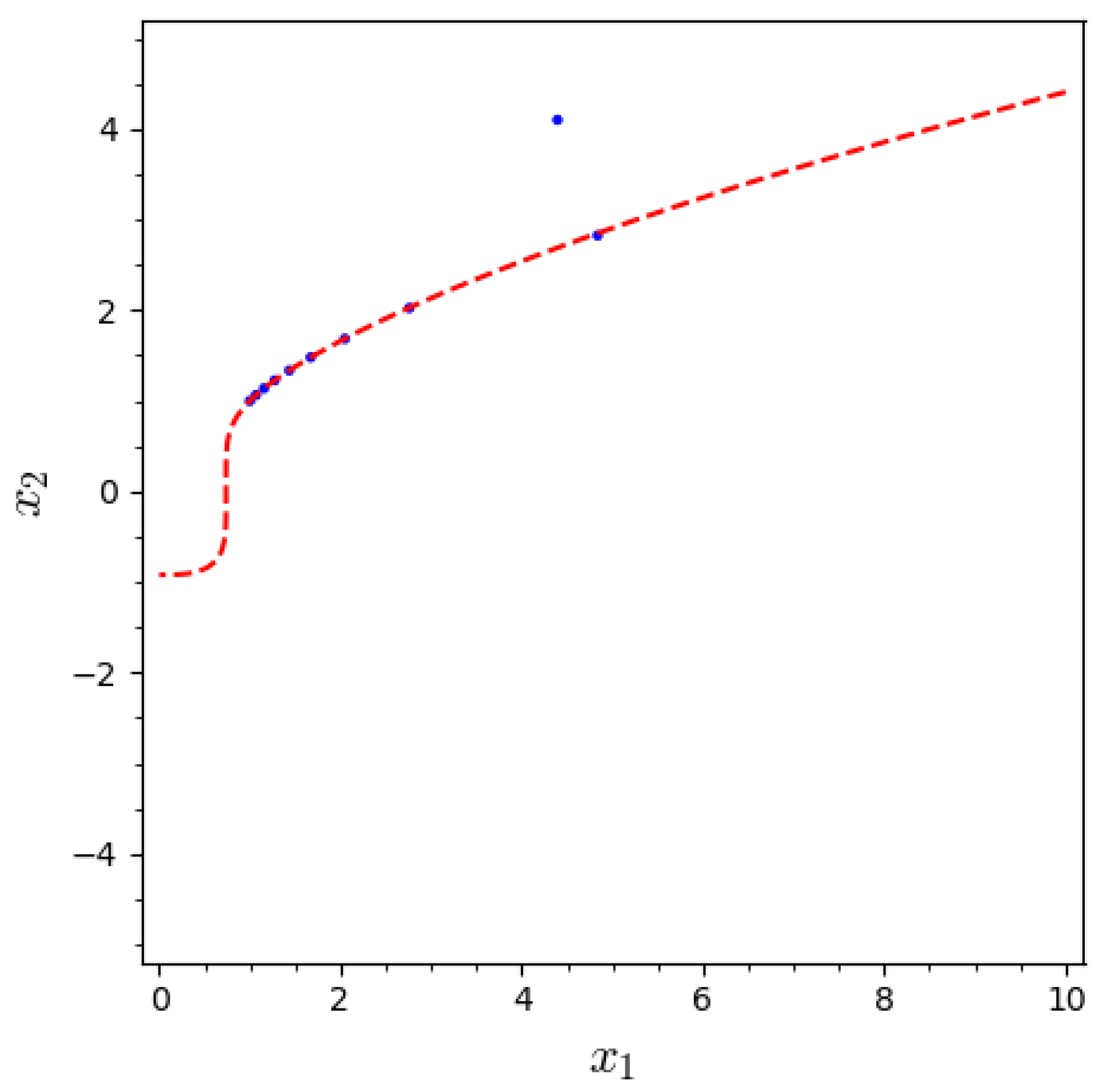
The particular solution of the system (12) with the initial conditions at has a branching point , the position of which was found numerically by standard means [22,24]. We found the solution (14) using Kahan’s method. In Figure 6, it is evident that almost all of its points lie with graphical accuracy on the integral curve (13), but some of them are noticeably off it. These points correspond to the value of t at which the integral relations connecting the variables and are noticeably violated. In Figure 7, it is clearly evident that at the branch point the auxiliary variables take on enormous values.

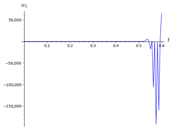
Figure 7.
Solution of system (14), obtained using the Kahan scheme.
7. Discussion of Results
For the equivalence of the original system of differential Equations (1) and the quadraticized system (3)–(5), these connections are very important, since the order of the systems is different: only on the corresponding integral manifold is the quadraticized system equivalent to the original one. The destruction of these connections means the loss of equivalence between the original system and the system obtained after Appelroth quadratization and Kahan discretization.
We can explain this as follows. The key advantage of Kahan’s method is to obtain a scheme that defines a one-to-one correspondence between the initial and final positions of the system. This leads to the inheritance of the difference scheme of integrals and other properties of the original dynamical system only if the original dynamical system has this property.
Elliptic oscillators have this property with reservations: the differential equations describing them define a birational correspondence to an algebraic integral variety. These correspondences do not extend to the Cremona transformation of the entire space, but can be approximated by such [12]. Of course, elliptic oscillators have the Painlevé property, i.e., they have no moving branch points.
Dynamical systems with a polynomial right-hand side, on the contrary, usually have moving branch points. This leads to the fact that the differential equations do not actually define a one-to-one correspondence between the initial and final states of the system, contrary to our expectations. Quadratization and discretization lead to a discrete model of the same system, which, however, differs from the original one precisely in that it defines a one-to-one correspondence between the initial and final states of the system. To achieve this, we sacrifice some algebraic properties of the original system of differential equations.
From the point of view of mathematical modeling, the question is not whether the discrete model corresponds as closely as possible to the continuous one, but whether its properties agree well with general principles and observations. Thus, two questions arise.
First, must a dynamical system always define a one-to-one correspondence? What physical meaning is hidden in the ambiguity of the correspondence between the initial and final data?
To answer this question, consider the Calogero system [25]. This system consists of n identical particles on a line, attracted to each other with a force inversely proportional to the cube of the distance. The coordinates of the particles are the roots of an n-th degree equation:
whose coefficients depend rationally on time and the initial positions and velocities of the bodies. In fact, we can find the coordinates of all n bodies algebraically, but we cannot figure out which is which. From a mathematical point of view, this means that the coordinate of the k-th body is a multi-valued analytic function of t, and the coordinates of the remaining bodies, that is, , are its branches. From a physical point of view, this means that all these bodies are identical, which brings us to the concept of algebrodynamics [26]. When modeling systems with many particles, one should not expect a one-to-one correspondence. When developing difference methods for studying such models, one can build into the difference model itself the kind of ambiguity that our system should have.
Second, are we always willing to sacrifice algebraic integrals to preserve birationality?
An interesting example from this point of view is offered by the gyroscope in the Lagrange case. In [9], it was shown that the integral expressing the equality of the sum of the squares of three direction cosines to 1, under Kahan discretization transforms into a relation of the form:
where c is the known rational function , which tends to 1 at . In other words, the one-to-oneness between the initial and final positions of the gyroscope has to be paid for by distorting the laws of Euclidean geometry. This is hardly applicable in classical mechanics. But then we should either look for other difference schemes for the top, or explain the physical meaning of the ambiguity that arises here.
8. Conclusions
Quadratization serves as a powerful, but little-studied tool in the analysis and numerical treatment of dynamical systems with polynomial right-hand sides. By transforming these systems into a quadratic form, researchers can leverage established numerical methods while preserving essential algebraic properties of the original equations or even imposing these properties forcibly. This structured approach not only enhances the understanding of dynamical systems, but also paves the way for future research in computational mathematics and related fields.
We believe that Appelroth’s quadratization provides important information about the Kahan method for differential equations with a quadratic right-hand side. In this way, we obtain dynamical systems with a quadratic right-hand side that have movable branch points. These systems inevitably have Darboux integrals that are destroyed by Kahan discretization. Therefore, Kahan discretization of systems with a quadratic right-hand side does not always lead to the inheritance of algebraic integrals and there is no need to even try to prove theorems about the inheritance of all algebraic integrals; they are obviously false.
The appropriateness of applying the combined Appelroth–Kahan approach to natural phenomena depends on which properties of these phenomena are important for research and which can be sacrificed. This approach is good if the one-to-one correspondence between the initial and final positions of the system is most important. Especially interesting is the case when the real system must define such a correspondence, but its continuous model using differential equations cannot have this property. As such a system, we can indicate an asymmetric gyroscope. Our approach allows to construct a difference scheme that approximates the original continuous model and at the same time define a birational correspondence between the initial and final positions.
This can be seen as a special case of a more general concept. Constructing difference schemes, we propose to move from the concept of inheritance of algebraic properties of a dynamical system (the idea of geometric integrators) to the concept of imposing of such properties, from the concept of mimeting a continuous model of a phenomenon—to the concept of creating a independent discrete model describing the same phenomenon.
Author Contributions
Conceptualization, L.S.; writing—original draft preparation, M.M. and L.L.; project administration, E.A. All authors have read and agreed to the published version of the manuscript.
Funding
The work of M. Malykh was supported by the RUDN University Strategic Academic Leadership Program, project No. 021934-0-000 (recipient M. Malykh, Section 4, Section 5 and Section 6). The work of E. Ayryan and L. Sevastianov was supported by the Russian Science Foundation (grant No. 20-11-20257, Section 1, Section 2, Section 3, Section 7 and Section 8).
Data Availability Statement
The original contributions presented in the study are included in the article, further inquiries can be directed to the corresponding author.
Conflicts of Interest
The authors declare no conflicts of interest.
References
- Appelroth, G.G. Die Normalform eines Systems von algebraischen Differentialgleichungen. Mat. Sb. 1902, 23, 12–23. [Google Scholar]
- Hemery, M.; Fages, F.; Soliman, S. On the complexity of quadratization for polynomial differential equations. In Proceedings of the Computational Methods in Systems Biology; Abate, A., Petrov, T., Wolf, V., Eds.; Springer: Cham, Switzerland, 2020; pp. 120–140. [Google Scholar] [CrossRef]
- Bychkov, A.; Pogudin, G. Optimal monomial quadratization for ODE systems. In Proceedings of the Combinatorial Algorithms; Flocchini, P., Moura, L., Eds.; Springer: Cham, Switzerland, 2021; pp. 122–136. [Google Scholar]
- Cai, Y.; Pogudin, G. Dissipative quadratizations of polynomial ODE systems. In Proceedings of the Tools and Algorithms for the Construction and Analysis of Systems; Finkbeiner, B., Kovács, L., Eds.; Springer: Cham, Switzerland, 2024; pp. 323–342. [Google Scholar] [CrossRef]
- Sanz-Serna, J.M. An unconventional symplectic integrator of W. Kahan. Appl. Numer. Math. 1994, 16, 245–250. [Google Scholar] [CrossRef]
- Celledoni, E.; McLachlan, R.I.; Owren, B.; Quispel, G.R.W. Geometric properties of Kahan’s method. J. Phys. A Math. Theor. 2013, 46, 025201. [Google Scholar] [CrossRef]
- Petrera, M.; Smirin, J.; Suris, Y.B. Geometry of the Kahan discretizations of planar quadratic Hamiltonian systems. Proc. R. Soc. A 2019, 475, 20180761. [Google Scholar] [CrossRef] [PubMed]
- Hirota, R.; Kimura, K. Discretization of the Euler top. J. Phys. Soc. Jpn. 2000, 69, 627–630. [Google Scholar] [CrossRef]
- Hirota, R.; Kimura, K. Discretization of the Lagrange top. J. Phys. Soc. Jpn. 2000, 69, 3193–3199. [Google Scholar] [CrossRef]
- Petrera, M.; Suris, Y.B. On the Hamiltonian structure of Hirota-Kimura discretization of the Euler top. Math. Nachr. 2010, 283, 1654–1663. [Google Scholar] [CrossRef]
- Ayrjan, E.A.; Malykh, M.D.; Sevastianov, L.A. On difference schemes approximating first-order differential equations and defining a projective correspondence between layers. J. Math. Sci. 2019, 240, 634–645. [Google Scholar] [CrossRef]
- Malykh, M.; Gambaryan, M.; Kroytor, O.; Zorin, A. Finite difference models of dynamical systems with quadratic right-hand side. Mathematics 2024, 12, 167. [Google Scholar] [CrossRef]
- Umemura, H. Birational automorphism groups and differential equations. Nagoya Math. J. 1990, 119, 1–80. [Google Scholar] [CrossRef]
- Malykh, M.D. On Transcendental Functions Arising from Integrating Differential Equations in Finite Terms. J. Math. Sci. 2015, 209, 935–952. [Google Scholar] [CrossRef]
- Severi, F. Lezioni di Geometria Algebrica; Angelo Graghi: Padova, Italy, 1908. [Google Scholar]
- Hairer, E.; Wanner, G.; Nørsett, S.P. Solving Ordinary Differential Equations I, 3rd ed.; Springer: Cham, Switzerland, 2008. [Google Scholar] [CrossRef]
- Kahan, W.; Li, R.-C. Unconventional schemes for a class of ordinary differential equations—With applications to the Korteweg–de Vries equation. J. Comput. Phys. 1997, 134, 316–331. [Google Scholar] [CrossRef]
- Petrera, M.; Pfadler, A.; Suris, Y.B.; Fedorov, Y.N. On the Construction of Elliptic Solutions of Integrable Birational Maps. Exp. Math. 2017, 26, 324–341. [Google Scholar] [CrossRef]
- Golubev, V.V. Lectures on Integration of the Equations of Motion of a Rigid Body about a Fixed Point; Israel Program for Scientific Translations: Jerusalem, Israel, 1960. [Google Scholar]
- Rerikh, K.V. Chew-Low equations as Cremona transformations structure of general intgrals. Jt. Inst. Nucl. Res. Dubna. Transl. Teor. Mat. Fiz. 1982, 50, 251–260. [Google Scholar] [CrossRef]
- Bychkov, A. QBee. 2021. Available online: https://github.com/AndreyBychkov/QBee (accessed on 28 August 2024).
- Baddour, A.; Gambaryan, M.M.; Gonzalez, L.; Malykha, M.D. On implementation of numerical methods for solving ordinary differential equations in computer algebra systems. Program. Comput. Soft. 2023, 49, 412–422. [Google Scholar] [CrossRef]
- Schlesinger, L. Einführung in die Theorie der Gewöhnlichen Differentialgleichungen auf Functionentheoretischer Grundlagen, 3rd ed.; Taubner: Berlin, Germany; Leipzig, Germany, 1922. [Google Scholar]
- Alshina, E.A.; Kalitkin, N.N.; Koryakin, P.V. Diagnostics of singularities of exact solutions in computations with error control. Comput. Math. Math. Phys. 2005, 45, 1769–1779. [Google Scholar]
- Moser, J. Integrable Hamiltonian Systems and Spectral Theory; Edizioni della Normale: Pisa, Italy, 1983. [Google Scholar]
- Kassandrov, V.V.; Khasanov, I.S. Algebrodynamics: Super-conservative collective dynamics on a “Unique worldline” and the Hubbleaw. Gravit. Cosmol. 2023, 29, 50–56. [Google Scholar] [CrossRef]

Disclaimer/Publisher’s Note: The statements, opinions and data contained in all publications are solely those of the individual author(s) and contributor(s) and not of MDPI and/or the editor(s). MDPI and/or the editor(s) disclaim responsibility for any injury to people or property resulting from any ideas, methods, instructions or products referred to in the content. |
© 2024 by the authors. Licensee MDPI, Basel, Switzerland. This article is an open access article distributed under the terms and conditions of the Creative Commons Attribution (CC BY) license (https://creativecommons.org/licenses/by/4.0/).