
Unified Modeling and Multi-Objective Optimization for Disassembly Line Balancing with Distinct Station Configurations


Abstract
:1. Introduction
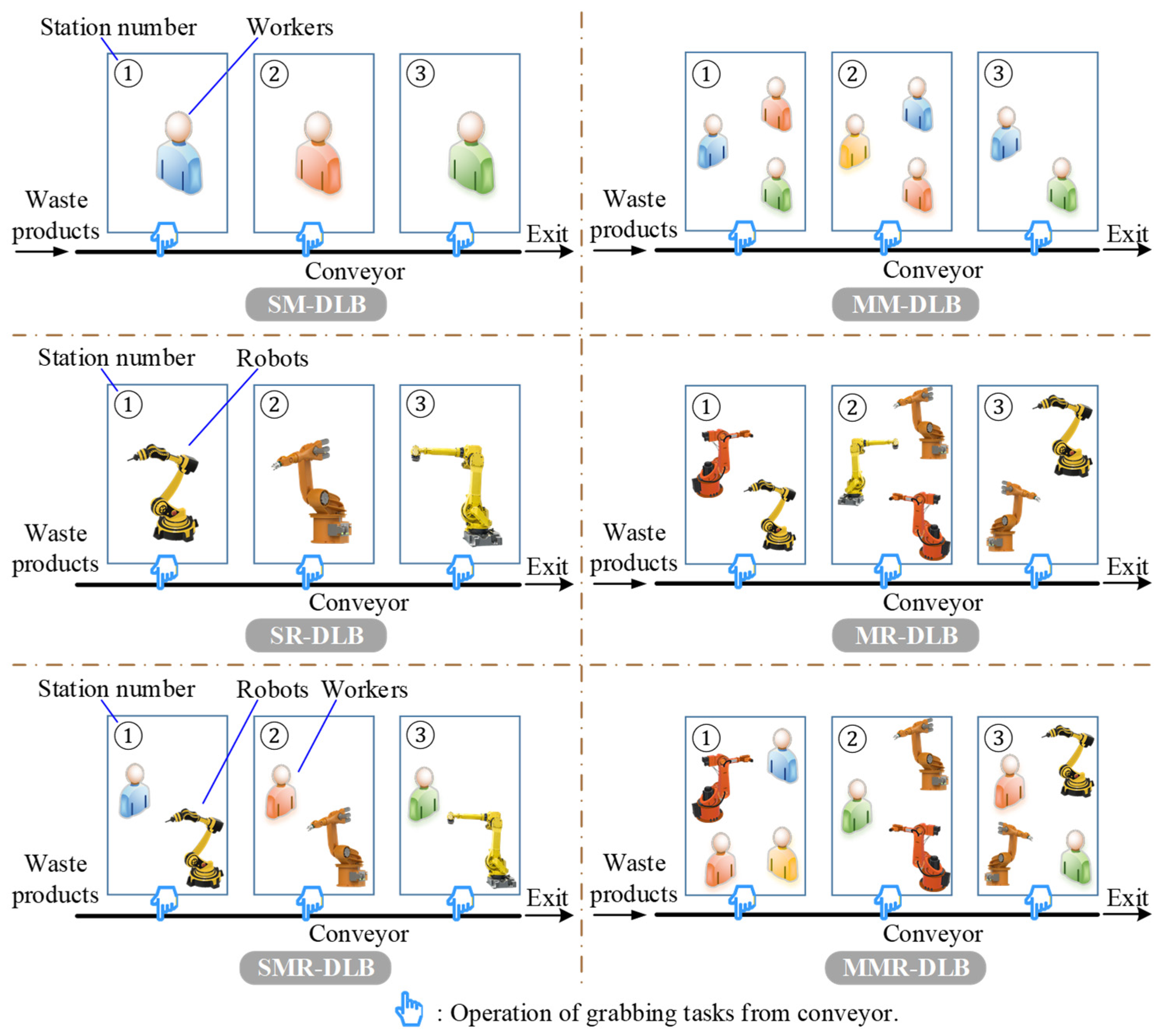
- Type-I and Type-II DLBs with six distinct operator configurations are unified, modeled, and solved by the mixed-integer programming approaches;
- Considering the efficiency difference between operators (workers and robots) makes the DLBs investigated more practical;
- In Type-I DLBs, a novel bi-metric is proposed to replace the idle balancing index to participate in lexicographic optimization, which can obtain more non-inferior solutions.
2. Related Work
3. Type-I DLB: Modelling and Optimization
| Indices: | |
| i, j | Task index. |
| k | Station index. |
| w | Worker index. |
| r | Robot index. |
| Sets and parameters: | |
| T | Task index set, i, j ∈ T. |
| K | Station index set, k ∈ K. |
| W | Worker index set, w ∈ W. |
| R | Robot index set, r ∈ R. |
| The maximum number of workers per station (h means human). | |
| The maximum number of robots per station (m means machine). | |
| CT | Cycle time. |
| KN | The number of the open station. |
| ON | The number of assigned operators. |
| TT | Total time to perform all tasks. |
| IB | Idle balancing index for assigned operators. |
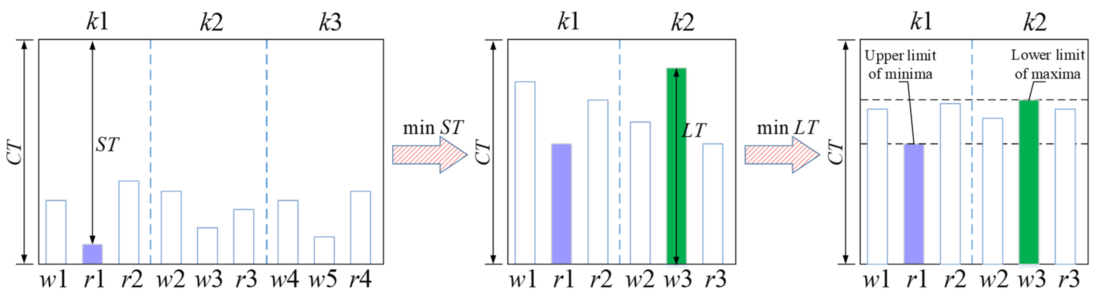
| ST | The maximum idle time of assigned operators. |
| LT | The maximum workload of assigned operators. |
| P(i) | Immediate predecessor set of task i. |
| ψ | A large positive number. |
| tiw | Time for worker w performing task i. Here, the processing time of each task performed by different workers is different due to the influence of the skill differences of workers. |
| tir | Time for robot r to perform task i. Here, the processing time of each task performed by different robots is different due to the influence of the performance differences. |
| ci | Complex attribute: 1, task i is too complex to be performed by robots; 0, otherwise. |
| hi | Hazardous attribute: 1, task i is harmful to workers; 0, otherwise. |
| Decision Variables: | |
| Start time of task i. | |
| Assignment of tasks to workers: 1, task i is assigned to worker w in station k; 0, otherwise. | |
| Assignment of tasks to robots: 1, task i is assigned to robot r in station k; 0, otherwise. | |
| Employment of workers: 1, worker w is assigned to station k; 0, otherwise. | |
| Employment of robots: 1, robot r is assigned to station k; 0, otherwise. | |
| Task ranking variable in workers: 1, task i and j are assigned to worker w in station k, and i is ranked before j; 0, otherwise. | |
| Task ranking variable in robots: 1, task i and j are assigned to robot r in station k, and i is ranked before j; 0, otherwise. | |
| sk | Station usage variable: 1, station k is used; 0, otherwise. |
| Mathematical operator: | |
| | | | Cardinal number of a set. |
3.1. Models of the Type-I DLBs with the Six Operator Configurations
3.1.1. Unified Model of the Type-I SMR-DLB and MMR-DLB
- (1)
- Optimization objectives:
- 1)
- The number of opened stations:
- 2)
- The number of assigned workers and robots:
- 3)
- The total performing time of all tasks by the assigned operators:
- 4)
- The idle balancing index for operators (the sum of squares of the idle time of each assigned worker and robot):
- (2)
- Constraints:
- 1)
- Because of the complete disassembly mode, each task is either performed by robots or workers (C1 represents the codename of the first constraint).
- 2)
- According to the task classification mentioned above, constraint C2 ensures that the complex tasks are only performed by workers, and constraint C3 ensures that the hazardous tasks are only performed by robots. Notably, when a task contains both complex and hazardous attributes, the task is still handed over to workers because robots cannot process the complex attribute; namely, the complex attribute of a task has a higher priority than its hazardous attribute, and this situation is included in constraint C2. In addition, because normal tasks can be performed by both workers and robots, they are not constrained, to ensure that they can be randomly distributed between the two types of operators.
- 3)
- In the disassembly process, the execution order of the tasks must meet their precedence relationships. Specifically, on the time axis with the start time of the first station as the zero point, the start time of the immediately following task should be greater than the end time of the immediately preceding task.
- 4)
- Each assigned worker or robot can only perform one task at a time; that is, the tasks assigned to one worker or robot are ordered. On the time axis, the start time of the tasks assigned to an operator later should be greater than the end time of the tasks first assigned to the operator. C5 constrains the execution order of tasks assigned to workers, and C6 constrains the execution order of tasks assigned to robots.
- 5)
- Owing to the limitation of cycle time, the starting point of the time at which each operator can start executing tasks is the end time of the previous station. Any task assigned to an operator should wait until all tasks assigned to the operator before that task are completed. Therefore, the start time of a task assigned to an operator should be greater than the sum of the time start point of the operator and the total performing time of all tasks assigned to the operator before the task, which is expressed by constraint C11. Evidently, the end time of a task cannot exceed the end time of the station where it is located, and this is expressed by constraint C12.
- 6)
- Because every task in the waste product must be performed, the first station must be opened. Starting from the second station, each subsequent station can be opened only when at least one task and at least one operator are assigned to the station; otherwise, it will not be opened. Thus, the total number of opened stations is at least one and does not exceed the minimum value of the total number of tasks and the total number of given operators, which can be ensured by constraint C13.
- 7)
- The SMR-DLB requires each station to employ at most one worker and one robot, whereas the MMR-DLB allows each station to employ multiple workers and robots. Thus, the variables and are used to limit the maximum number of operators assigned to each station. When = 1 and = 1, this model can be used to solve the SMR-DLB, and when > 1 or > 1, this model can be used to solve the MMR-DLB. Such limitations can be imposed by constraints C16 and C17.
- 8)
- Constraint C22 lists all the binary variables used in the model.
3.1.2. Unified Model of the Type-I SM-DLB, MM-DLB, SR-DLB, and MR-DLB
- Kept: f1, C5, C7–C8, C15–C16, C18, C20;
- Removed: C2–C3, C6, C9–C10, C17, C19, C21;
- Modified: f2–f4, C1, C4, C11–C14, C22.
- The modified parts are executed in detail below:
- (1)
- Optimization objective:
- (2)
- Constraints:
3.1.3. A Bi-Metric to Replace Quadratic Idle Balancing Index
3.2. Actual Case Calculation and Verification
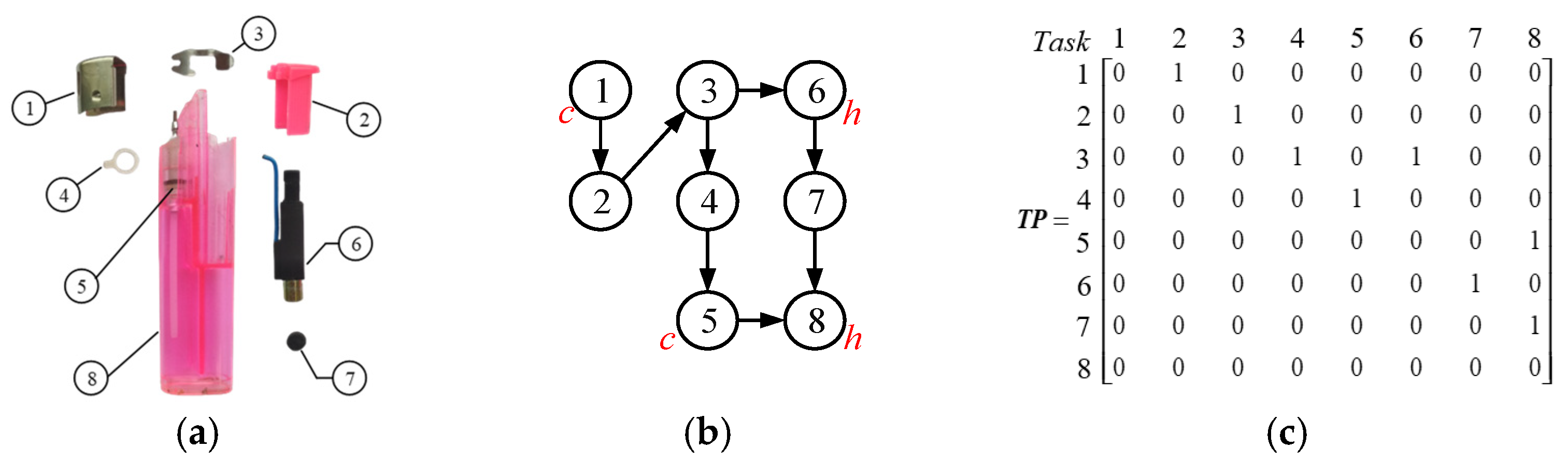
3.2.1. Case I: Lighter
- (1)
- Basic disassembly information:
- (2)
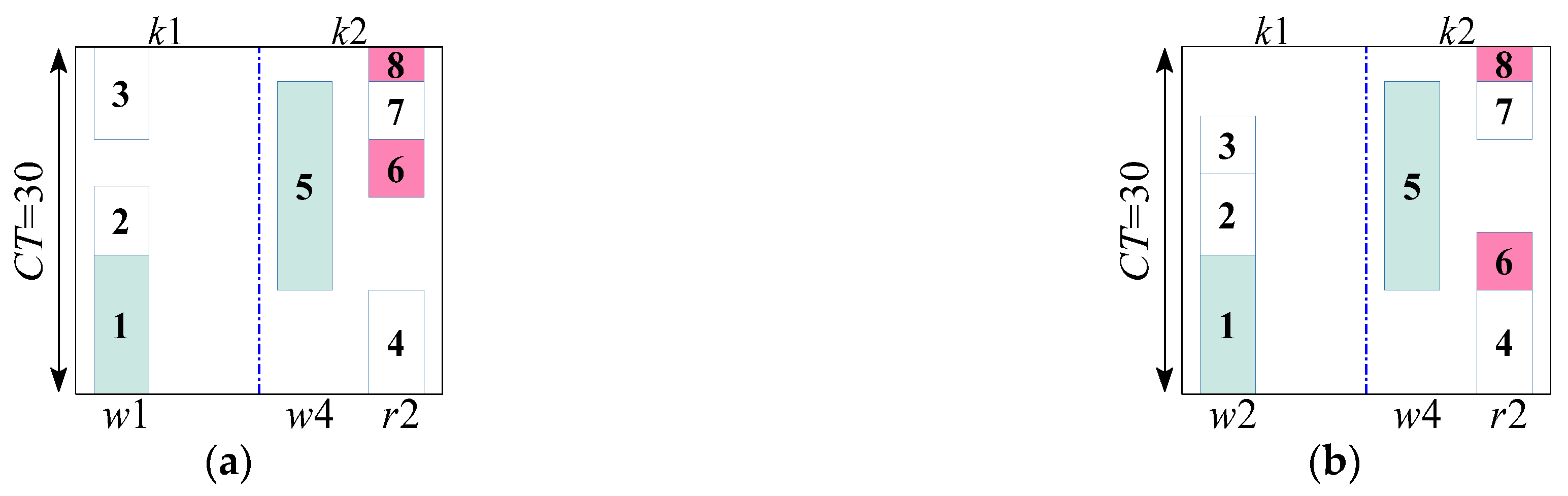
- Optimization results and analysis:
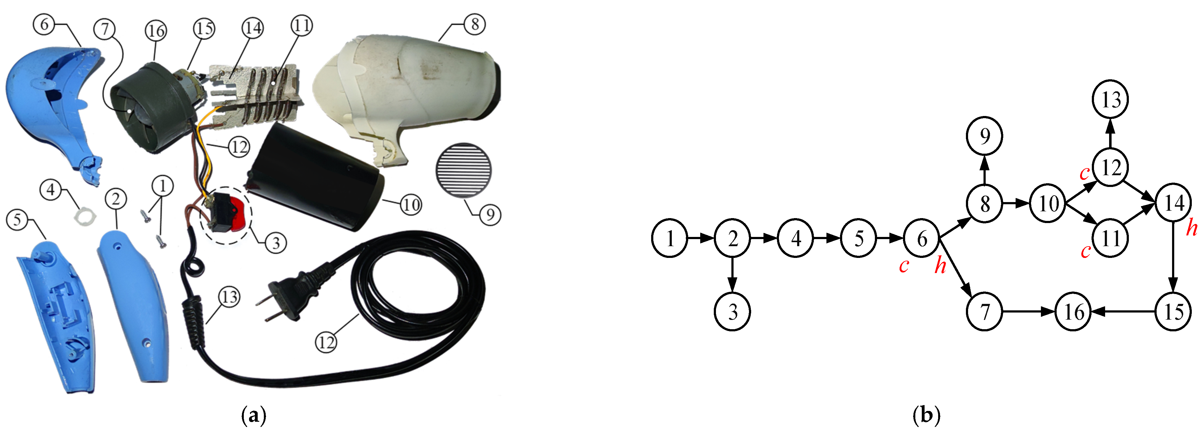
3.2.2. Case II: Hairdryer
- (1)
- Basic disassembly information:
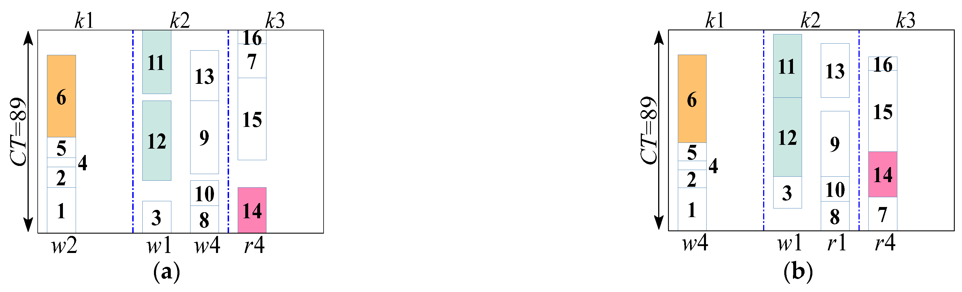
- (2)
- Optimization results and analysis:
3.3. Discussion for Type-I DLBs
4. Type-II DLB: Modelling and Optimization
4.1. Models of the Type-II DLB with the Six Operator Configurations
4.1.1. Unified Model of the Type-II SMR-DLB and MMR-DLB
- (1)
- Optimization objectives:
- (2)
- Constraints:
4.1.2. Unified Model of the Type-II SM-DLB, MM-DLB, SR-DLB, and MR-DLB
- (1)
- Optimization objectives: = ff1, = , = , = .
- (2)
- Constraints:Selected: , , C5, C7–C8, CC11–CC12, , C15–C16, C18, C20, ;
4.2. Partial Linearization and Results Presentation
4.2.1. Partial Linearization for the Idle Balancing Index
4.2.2. Cases I and II: Lighter and Hairdryer
4.3. Discussion for Type-II DLBs
5. Conclusions and Future Work
Supplementary Materials
Author Contributions
Funding
Data Availability Statement
Conflicts of Interest
Appendix A

| MMR-DLB ( = 3 and = 2) | |||||||||
|---|---|---|---|---|---|---|---|---|---|
| No. | f1 | f2 | f3 | f4 | f5 | f6 | Priority Order of Objectives f (Time/s) | Notes | |
| Original model | 1 | 3 | 4 | 321 | 373 | 12 | 87 | 4(5257.78). | - |
| 2 | 2 | 4 | 284 | 1794 | - | - | 123(11.00), 213(27.03). | - | |
| 3 | 2 | 6 | 263 | 13,231 | - | - | 132(10.68). | - | |
| 4 | 3 | 4 | 273 | 2609 | - | - | 231(46.50). | - | |
| 5 | 3 | 7 | 262 | 22,327 | - | - | 312(19.98), 321(32.11). | - | |
| Bi-metric method | 6 | 3 | 4 | 309 | 553 | 12 | 78 | 56(323.75). | Non-inferior to No.1 |
| 7 | 2 | 4 | 284 | 1794 | 28 | 88 | 15,623(26.75), 15,632(26.83), 12,563(23.31), 12,356(23.28), 21,563(90.20), 21,356(100.38). | Same as No.2 | |
| 8 | 2 | 6 | 263 | 13,231 | 63 | 61 | 13,562(22.13), 13,256(21.56). | Same as No.3 | |
| 9 | 3 | 4 | 273 | 2609 | 42 | 85 | 23,561(260.98), 23,156(286.91). | Same as No.4 | |
| 10 | 3 | 4 | 309 | 553 | 12 | 78 | 56,123(149.73), 56,132(150.13), 56,213(159.53), 56,231(174.19), 56,312(164.20), 56,321(174.38), 25,613(213.39), 25,631(225.34). | Same as No.6 | |
| 11 | 3 | 7 | 262 | 22,327 | 85 | 85 | 35,612(118.24), 35,621(136.42), 31,562(42.22), 31,256(50.06), 32,561(125.14), 32,156(56.48). | Same as No.5 | |
| SMR-DLB ( = 1 and = 1) | |||||||||
| Original model | 1 | 3 | 4 | 321 | 373 | 12 | 87 | 4(2449.86) | - |
| 2 | 3 | 4 | 273 | 2609 | - | - | 231(38.17). | - | |
| 3 | 3 | 4 | 273 | 2613 | - | - | 123(15.41). | Inferior to No.2 | |
| 4 | 3 | 4 | 273 | 3157 | - | - | 213(33.58). | Inferior to No.2,3 | |
| 5 | 3 | 6 | 265 | 14,279 | - | - | 132(13.88). | - | |
| 6 | 4 | 7 | 262 | 22,327 | - | - | 312(22.45), 321(29.11). | - | |
| Bi-metric method | 7 | 3 | 4 | 309 | 553 | 12 | 78 | 56(111.86). | Non-inferior to No.1 |
| 8 | 3 | 4 | 273 | 2609 | 42 | 85 | 12,356(40.94), 21,356(71.70), 23,561(195.31), 23,156(81.92). | Same as No.2 | |
| 9 | 3 | 4 | 309 | 553 | 12 | 78 | 56,123(159.56), 56,132(153.38), 56,213(164.63), 56,231(182.97), 56,312(168.44), 56,321(184.13), 15,623(27.22), 15,632(36.13), 12,563(41.89), 25,613(142.53), 25,631(164.25), 21,563(100.95). | Same as No.6 | |
| 10 | 3 | 6 | 265 | 14,279 | 63 | 80 | 13,562(31.86), 13,256(35.27). | Same as No.5 | |
| 11 | 4 | 7 | 262 | 22,327 | 85 | 85 | 35,612(141.06), 35,621(156.56), 31,562(52.61), 31,256(57.64), 32,561(123.53), 32,156(80.09). | Same as No.6 | |
| MM-DLB ( = 3) | |||||||||
| Original model | 1 | 3 | 4 | 317 | 473 | 15 | 87 | 4(794.23). | - |
| 2 | 2 | 5 | 280 | 7651 | - | - | 123(2.22), 132(2.23). | - | |
| 3 | 3 | 4 | 277 | 2799 | - | - | 213(4.94). | - | |
| 4 | 3 | 4 | 277 | 2853 | - | - | 231(6.98). | Inferior to No.3 | |
| 5 | 3 | 5 | 276 | 9731 | - | - | 321(6.36). | - | |
| 6 | 3 | 5 | 276 | 9785 | - | - | 312(4.61). | Inferior to No.5 | |
| Bi-metric method | 7 | 3 | 4 | 304 | 692 | 15 | 78 | 56(7.53). | Non-inferior to No.1 |
| 8 | 2 | 5 | 280 | 7651 | 65 | 84 | 12,356(3.41), 13,562(3.47), 13,256(3.44). | Same as No.2 | |
| 9 | 2 | 5 | 289 | 5076 | 39 | 68 | 15,623(3.42), 15,632(3.45), 12,563(3.40). | New solution | |
| 10 | 3 | 4 | 277 | 2799 | 50 | 82 | 21,356(7.52), 23,561(12.80), 23,156(9.33). | Same as No.3 | |
| 11 | 3 | 4 | 300 | 796 | 15 | 78 | 56,123(13.53), 56,132(13.90), 56,213(13.97), 56,231(16.10), 56,312(15.89), 56,321(16.38), 25,613(12.31), 25,631(13.76), 21,563(10.06). | New solution | |
| 12 | 3 | 5 | 276 | 9731 | 82 | 82 | 35,612(11.97), 35,621(13.40), 31,562(7.50), 31,256(7.14), 32,561(13.45), 32,156(8.74) | Same as No.5 | |
| SM-DLB ( = 1) | |||||||||
| Original model | 1 | 4 | 4 | 316 | 494 | 15 | 87 | 4(156.94). | - |
| 2 | 4 | 4 | 278 | 2854 | - | - | 123(4.46), 132(4.09), 213(4.50), 231(5.64). | - | |
| 3 | 5 | 5 | 276 | 9785 | - | - | 312(5.12), 321(5.42). | - | |
| Bi-metric method | 4 | 4 | 4 | 307 | 611 | 15 | 78 | 56(3.81). | Non-inferior to No.1 |
| 5 | 4 | 4 | 278 | 2854 | 50 | 85 | 12,356(5.44), 13,562(5.66), 13,256(5.87), 21,356(5.92), 23,561(7.46), 23,156(6.81). | Same as No.2 | |
| 6 | 4 | 4 | 304 | 686 | 15 | 78 | 56,123(6.51), 56,132(6.46), 56,213(6.75), 56,312(7.07), 56,321(7.33), 25,613(6.57), 25,631(6.73). | New solution | |
| 7 | 4 | 4 | 304 | 692 | 15 | 78 | 56,231(7.01), 15,623(5.86), 15,632(6.08), 12,563(6.18), 21,563(7.10). | Inferior to No.6 | |
| 8 | 5 | 5 | 276 | 9785 | 82 | 85 | 35,612(9.88), 35,621(9.78), 31,562(8.02), 31,256(8.81), 32,561(9.46), 32,156(9.71). | Same as No.3 | |
| MR-DLB ( = 2) | |||||||||
| Original model | 1 | 3 | 4 | 311 | 533 | 15 | 81 | 4(94.94). | - |
| 2 | 2 | 4 | 275 | 3049 | - | - | 123(1.14), 132(1.17), 213(1.90). | - | |
| 3 | 3 | 4 | 270 | 2186 | - | - | 231(2.96), 312(2.11), 321(3.01). | - | |
| Bi-metric method | 4 | 3 | 4 | 309 | 557 | 13 | 79 | 56(3.05). | Non-inferior to No.1 |
| 5 | 2 | 4 | 275 | 3049 | 40 | 88 | 15,623(1.84),15,632(1.86), 12,563(1.81), 12,356(1.79), 13,562(1.80), 13,256(1.80), 21,563(3.06), 21,356(2.69). | Same as No.2 | |
| 6 | 3 | 4 | 270 | 2186 | 30 | 83 | 23,561(4.70), 23,156(4.05), 35,612(3.92), 35,621(3.91), 31,562(3.78), 31,256(3.70), 32,561(4.06), 32,156(4.09). | Same as No.3 | |
| 7 | 3 | 4 | 308 | 582 | 13 | 79 | 56,123(4.96), 56,132(5.32), 56,213(5.47), 56,231(5.79), 56,312(5.61), 56,321(5.77), 25,613(5.51), 25,631(6.11). | New solution | |
| SR-DLB ( = 1) | |||||||||
| Original model | 1 | 4 | 4 | 310 | 618 | 18 | 84 | 4(4.88). | - |
| 2 | 4 | 4 | 272 | 2666 | - | - | 123(2.52), 132(2.41), 213(2.53), 231(2.42), 312(2.30), 321(2.03). | - | |
| Bi-metric method | 3 | 4 | 4 | 301 | 777 | 16 | 79 | 56(2.11). | Non-inferior to No.1 |
| 4 | 4 | 4 | 301 | 777 | 16 | 79 | 56,123(3.38), 56,132(3.36), 56,213(3.42), 56,231(3.39), 56,312(3.45), 56,321(3.55), 15,623(4.00), 15,632(3.88), 12,563(4.45), 25,613(3.42), 25,631(3.44), 21,563(4.09). | Same as No.3 | |
| 5 | 4 | 4 | 272 | 2666 | 41 | 83 | 12,356(4.42), 13,562(3.64), 13,256(3.55), 21,356(4.67), 23,561(4.33), 23,156(3.94), 35,612(3.75), 35,621(3.72), 31,562(4.00), 31,256(3.72), 32,561(3.66), 32,156(3.84). | Same as No.2 |
References
- Khakbaz, A.; Tirkolaee, E.B. A sustainable hybrid manufacturing/remanufacturing system with two-way substitution and WEEE directive under different market conditions. Optimization 2021, 71, 3083–3106. [Google Scholar] [CrossRef]
- Dong, J.; Jiang, L.; Lu, W.; Guo, Q. Closed-loop supply chain models with product remanufacturing under random demand. Optimization 2021, 70, 27–53. [Google Scholar] [CrossRef]
- Lu, Q.; Ren, Y.; Jin, H.; Meng, L.; Li, L.; Zhang, C.; Sutherland, J.W. A hybrid metaheuristic algorithm for a profit-oriented and energy-efficient disassembly sequencing problem. Robot. Comput. Manuf. 2020, 61, 101828. [Google Scholar] [CrossRef]
- Zhu, L.; Zhang, Z.; Wang, Y. A Pareto firefly algorithm for multi-objective disassembly line balancing problems with hazard evaluation. Int. J. Prod. Res. 2018, 56, 7354–7374. [Google Scholar] [CrossRef]
- Koc, A.; Sabuncuoglu, I.; Erel, E. Two exact formulations for disassembly line balancing problems with task precedence diagram construction using an AND/OR graph. IIE Trans. 2009, 41, 866–881. [Google Scholar] [CrossRef]
- Güler, E.; Kalayci, C.B.; Ilgin, M.A.; Özceylan, E.; Güngör, A. Advances in partial disassembly line balancing: A state-of-the-art review. Comput. Ind. Eng. 2024, 188, 109898. [Google Scholar] [CrossRef]
- Yin, T.; Zhang, Z.; Liang, W.; Zeng, Y.; Zhang, Y. Multi-man–robot disassembly line balancing optimization by mixed-integer programming and problem-oriented group evolutionary algorithm. IEEE Trans. Syst. Man Cybern. Syst. 2024, 54, 1363–1375. [Google Scholar] [CrossRef]
- Xu, W.; Tang, Q.; Liu, J.; Liu, Z.; Zhou, Z.; Pham, D.T. Disassembly sequence planning using discrete Bees algorithm for human-robot collaboration in remanufacturing. Robot. Comput. Integr. Manuf. 2020, 62, 101860. [Google Scholar] [CrossRef]
- Wu, T.; Zhang, Z.; Yin, T.; Zhang, Y. Multi-objective optimisation for cell-level disassembly of waste power battery modules in human-machine hybrid mode. Waste Manag. 2022, 144, 513–526. [Google Scholar] [CrossRef]
- Ding, Y.; Xu, W.; Liu, Z. Robotic task oriented knowledge graph for human-robot collaboration in disassembly. Procedia CIRP 2019, 83, 105–110. [Google Scholar] [CrossRef]
- Liu, Q.; Liu, Z.; Xu, W.; Tang, Q.; Zhou, Z.; Pham, D.T. Human-robot collaboration in disassembly for sustainable manufacturing. Int. J. Prod. Res. 2019, 57, 4027–4044. [Google Scholar] [CrossRef]
- Huang, J.; Pham, D.T.; Wang, Y.; Qu, M.; Ji, C.; Su, S.; Xu, W.; Liu, Q.; Zhou, Z. A case study in human–robot collaboration in the disassembly of press-fitted components. Proc. Inst. Mech. Eng. Part B J. Eng. Manuf. 2020, 234, 654–664. [Google Scholar] [CrossRef]
- Laili, Y.; Li, Y.; Fang, Y.; Pham, D.T.; Zhang, L. Model review and algorithm comparison on multi-objective disassembly line balancing. J. Manuf. Syst. 2020, 56, 484–500. [Google Scholar] [CrossRef]
- Deniz, N.; Ozcelik, F. An extended review on disassembly line balancing with bibliometric & social network and future study realization analysis. J. Clean. Prod. 2019, 225, 697–715. [Google Scholar] [CrossRef]
- Özceylan, E.; Kalayci, C.B.; Güngör, A.; Gupta, S.M. Disassembly line balancing problem: A review of the state of the art and future directions. Int. J. Prod. Res. 2019, 57, 4805–4827. [Google Scholar] [CrossRef]
- Pour-Massahian-Tafti, M.; Godichaud, M.; Amodeo, L. Disassembly EOQ models with price-sensitive demands. Appl. Math. Model. 2020, 88, 810–826. [Google Scholar] [CrossRef]
- Yin, T.; Zhang, Z.; Zhang, Y. Mixed-integer programming model and hybrid driving algorithm for multi-product partial disassembly line balancing problem with multi-robot stations. Robot. Comput. Integr. Manuf. 2022, 73, 102251. [Google Scholar] [CrossRef]
- Ibrahim, K.; Zixiang, L.; Yuchen, L. Type-E disassembly line balancing problem Type-E disassembly line balancing problem with multi-manned station. Optim. Eng. 2020, 21, 611–630. [Google Scholar] [CrossRef]
- He, J.; Chu, F.; Dolgui, A.; Anjos, M.F. Multi-objective disassembly line balancing and related supply chain management problems under uncertainty: Review and future trends. Int. J. Prod. Econ. 2024, 272, 109257. [Google Scholar] [CrossRef]
- Gao, J.; Wang, G.; Xiao, J.; Zheng, P.; Pei, E. Partially observable deep reinforcement learning for multi-agent strategy optimization of human-robot collaborative disassembly: A case of retired electric vehicle battery. Robot. Comput. Integr. Manuf. 2024, 89, 102775. [Google Scholar] [CrossRef]
- Djenadi, A.; Khanouche, M.E.; Mendil, B. A lexicographic optimization-based approach for efficient task allocation in industrial transportation multi-robot systems. Expert Syst. Appl. 2024, 257, 124998. [Google Scholar] [CrossRef]
- McGovern, S.M.; Gupta, S.M. Unified assembly- and disassembly-line model formulae. J. Manuf. Technol. Manag. 2015, 26, 195–212. [Google Scholar] [CrossRef]
- Mcgovern, S.M.; Gupta, S.M. Combinatorial optimization analysis of the unary NP-complete disassembly line balancing problem. Int. J. Prod. Res. 2007, 45, 4485–4511. [Google Scholar] [CrossRef]
- McGovern, S.M.; Gupta, S.M. 2-Opt Heuristic for the Disassembly Line Balancing Problem. Environ. Conscious Manuf. III 2004, 5262, 71–84. [Google Scholar]
- Gungor, A.; Gupta, S.M. A solution approach to the disassembly line balancing problem in the presence of task failures. Int. J. Prod. Res. 2001, 39, 1427–1467. [Google Scholar] [CrossRef]
- Chand, M.; Ravi, C. An optimal disassembly sequence planning for complex products using enhanced deep reinforcement learning framework. SN Comput. Sci. 2024, 5, 581. [Google Scholar] [CrossRef]
- Guo, X.; Zhou, M.; Liu, S.; Qi, L. Lexicographic Multiobjective Scatter Search for the Optimization of Sequence-Dependent Selective Disassembly Subject to Multiresource Constraints. IEEE Trans. Cybern. 2020, 50, 3307–3317. [Google Scholar] [CrossRef]
- Ming, H.; Liu, Q.; Pham, D.T. Multi-Robotic Disassembly Line Balancing with Uncertain Processing Time. Procedia CIRP 2019, 83, 71–76. [Google Scholar] [CrossRef]
- Altekin, F.T.; Kandiller, L.; Ozdemirel, N.E. Profit-oriented disassembly-line balancing. Int. J. Prod. Res. 2008, 46, 2675–2693. [Google Scholar] [CrossRef]
- Guo, X.; Liu, S.; Zhou, M.; Tian, G. Dual-Objective Program and Scatter Search for the Optimization of Disassembly Sequences Subject to Multiresource Constraints. IEEE Trans. Autom. Sci. Eng. 2018, 15, 1091–1103. [Google Scholar] [CrossRef]
- Guo, X.; Liu, S.; Zhou, M.; Tian, G. Disassembly sequence optimization for large-scale products with multiresource constraints using scatter search and petri nets. IEEE Trans. Cybern. 2015, 46, 2435–2446. [Google Scholar] [CrossRef]
- Gupta, S.M.; Güngör, A. Product recovery using a disassembly line: Challenges and solution. In Proceedings of the 2001 IEEE International Symposium on Electronics and the Environment, Denver, CO, USA, 9 May 2001; pp. 36–40. [Google Scholar]
- Ren, Y.; Zhang, C.; Zhao, F.; Triebe, M.J.; Meng, L. An MCDM-Based Multiobjective General Variable Neighborhood Search Approach for Disassembly Line Balancing Problem. IEEE Trans. Syst. Man Cybern. Syst. 2020, 50, 3770–3783. [Google Scholar] [CrossRef]
- Wang, K.; Li, X.; Gao, L.; Li, P. Modeling and Balancing for Disassembly Lines Considering Workers with Different Efficiencies. IEEE Trans. Cybern. 2021, 52, 11758–11771. [Google Scholar] [CrossRef]
- Cevikcan, E.; Aslan, D.; Yeni, F.B. Disassembly line design with multi-manned stations: A novel heuristic optimization approach. Int. J. Prod. Res. 2020, 58, 649–670. [Google Scholar] [CrossRef]
- Çil, Z.A. An exact solution method for multi-manned disassembly line design with AND/OR precedence relations. Appl. Math. Model. 2021, 99, 785–803. [Google Scholar] [CrossRef]
- Yılmaz, F.; Yazıcı, B. Tactical level strategies for multi-objective disassembly line balancing problem with multi-manned stations: An optimization model and solution approaches. Ann. Oper. Res. 2021, 319, 1793–1843. [Google Scholar] [CrossRef]
- Liu, B.; Xu, W.; Liu, J.; Yao, B.; Zhou, Z.; Pham, D.T. Human-robot collaboration for disassembly line balancing problem in remanufacturing. In Proceedings of the ASME 2019 14th International Manufacturing Science and Engineering Conference, Erie, PA, USA, 10–14 June 2019; Volume 1, pp. 1–8. [Google Scholar]
- Xu, C.; Wei, H.; Guo, X.; Liu, S.; Qi, L.; Zhao, Z. Human-Robot Collaboration Multi-Objective Disassembly Line Balancing Subject to Task Failure via Multi-Objective Artificial Bee Colony Algorithm. IFAC-PapersOnLine 2020, 53, 1–6. [Google Scholar] [CrossRef]
- Liu, J.; Zhou, Z.; Pham, D.T.; Xu, W.; Ji, C.; Liu, Q. Collaborative optimization of robotic disassembly sequence planning and robotic disassembly line balancing problem using improved discrete Bees algorithm in remanufacturing. Robot. Comput. Integr. Manuf. 2020, 61, 1879–2537. [Google Scholar] [CrossRef]
- Liu, J.; Zhou, Z.; Pham, D.T.; Xu, W.; Yan, J.; Liu, A.; Ji, C.; Liu, Q. An improved multi-objective discrete bees algorithm for robotic disassembly line balancing problem in remanufacturing. Int. J. Adv. Manuf. Technol. 2018, 97, 3937–3962. [Google Scholar] [CrossRef]
- Çil, Z.A.; Mete, S.; Serin, F. Robotic disassembly line balancing problem: A mathematical model and ant colony optimization approach. Appl. Math. Model. 2020, 86, 335–348. [Google Scholar] [CrossRef]
- Fang, Y.; Liu, Q.; Li, M. Evolutionary many-objective optimization for mixed-model disassembly line balancing with multi-robotic stations. Eur. J. Oper. Res. 2019, 276, 160–174. [Google Scholar] [CrossRef]
- Fang, Y.; Wei, H.; Liu, Q.; Li, Y.; Zhou, Z.; Pham, D.T. Minimizing energy consumption and line length of mixed-model multirobotic disassembly line systems using multi-objective evolutionary optimization. In Proceedings of the ASME 2019 14th International Manufacturing Science and Engineering Conference, Erie, PA, USA, 10–14 June 2019; Volume 1, pp. 1–10. [Google Scholar]
- Fang, Y.; Xu, H.; Liu, Q.; Pham, D.T. Evolutionary optimization using epsilon method for resource-constrained multi-robotic disassembly line balancing. J. Manuf. Syst. 2020, 56, 392–413. [Google Scholar] [CrossRef]
- Fang, Y.; Ming, H.; Li, M.; Liu, Q.; Pham, D.T. Multi-objective evolutionary simulated annealing optimisation for mixed-model multi-robotic disassembly line balancing with interval processing time. Int. J. Prod. Res. 2020, 58, 846–862. [Google Scholar] [CrossRef]
- Liu, Q.; Li, Y.; Fang, Y.; Laili, Y.; Lou, P.; Pham, D.T. Many-objective best-order-sort genetic algorithm for mixed-model multi-robotic disassembly line balancing. Procedia CIRP 2019, 83, 14–21. [Google Scholar] [CrossRef]
- Zhu, L.; Zhang, Z.; Wang, Y. On the end-of-life state oriented multi-objective disassembly line balancing problem. J. Intell. Manuf. 2020, 31, 1403–1428. [Google Scholar] [CrossRef]
- Wang, K.; Li, X.; Gao, L.; Li, P. Modeling and Balancing for Green Disassembly Line Using Associated Parts Precedence Graph and Multi-objective Genetic Simulated Annealing. Int. J. Precis. Eng. Manuf. Technol. 2020, 8, 1597–1613. [Google Scholar] [CrossRef]
- Agrawal, S.; Tiwari, M.K. A collaborative ant colony algorithm to stochastic mixed-model U-shaped disassembly line balancing and sequencing problem. Int. J. Prod. Res. 2008, 46, 1405–1429. [Google Scholar] [CrossRef]
- Wang, K.; Li, X.; Gao, L. A multi-objective discrete flower pollination algorithm for stochastic two-sided partial disassembly line balancing problem. Comput. Ind. Eng. 2019, 130, 634–649. [Google Scholar] [CrossRef]
- Zhu, L.; Zhang, Z.; Guan, C. Multi-objective partial parallel disassembly line balancing problem using hybrid group neighbourhood search algorithm. J. Manuf. Syst. 2020, 56, 252–269. [Google Scholar] [CrossRef]
- Yin, T.; Zhang, Z.; Jiang, J. A Pareto-discrete hummingbird algorithm for partial sequence-dependent disassembly line balancing problem considering tool requirements. J. Manuf. Syst. 2021, 60, 406–428. [Google Scholar] [CrossRef]
| Tasks | Workers (tiw) | Robots (tir) | |||||
|---|---|---|---|---|---|---|---|
| 1 | 2 | 3 | 4 | 1 | 2 | 3 | |
| 1 | 12 | 12 | 14 | 13 | 14 | 12 | 13 |
| 2 | 6 | 7 | 5 | 6 | 3 | 5 | 3 |
| 3 | 8 | 5 | 6 | 6 | 7 | 9 | 8 |
| 4 | 11 | 12 | 10 | 12 | 7 | 9 | 11 |
| 5 | 16 | 15 | 17 | 18 | 18 | 17 | 16 |
| 6 | 6 | 9 | 5 | 8 | 4 | 5 | 3 |
| 7 | 5 | 4 | 6 | 7 | 3 | 5 | 4 |
| 8 | 7 | 4 | 5 | 6 | 5 | 3 | 5 |
| MMR-DLB ( = 2 and = 2) | |||||||||
|---|---|---|---|---|---|---|---|---|---|
| No. | f1 | f2 | f3 | f4 | f5 | f6 | Priority Order of Objectives f (Time/s) | Notes | |
| Original model | 1 | 2 | 3 | 66 | 224 | 12 | 26 | 4(1.72). | - |
| 2 | 2 | 3 | 59 | 353 | - | - | 123(0.47), 231(1.08). | - | |
| 3 | 2 | 3 | 59 | 371 | - | - | 213(0.59). | Inferior to No.2 | |
| 4 | 2 | 5 | 52 | 2112 | - | - | 132(0.48). | - | |
| 5 | 3 | 5 | 51 | 2129 | - | - | 312(0.33), 321(0.34). | - | |
| Bi-metric method | 6 | 2 | 3 | 64 | 244 | 12 | 24 | 56(1.72). | Non-inferior to No.1 |
| 7 | 2 | 3 | 59 | 353 | 14 | 24 | 12,356(1.38), 21,356(1.78), 23,561(2.36), 23,156(1.78). | Same as No.2 | |
| 8 | 2 | 3 | 61 | 301 | 12 | 24 | 56,123(1.98), 56,132(1.95), 56,213(2.08), 56,231(2.30), 56,312(2.08), 56,321(2.24), 15,623(1.26), 15,632(1.23), 12,563(1.25), 25,613(1.89), 25,631(1.95), 21,563(1.56). | New solution | |
| 9 | 2 | 5 | 52 | 2070 | 27 | 17 | 13,256(1.03). | Dominates No.4 | |
| 10 | 2 | 6 | 52 | 2830 | 27 | 15 | 13,562(1.05). | Inferior to No.9 | |
| 11 | 3 | 5 | 51 | 2129 | 27 | 20 | 35,612(1.13), 35,621(1.09). | Same as No.5 | |
| 12 | 3 | 5 | 51 | 2171 | 27 | 20 | 31,562(0.94), 31,256(0.94), 32,561(0.91), 32,156(0.92). | Inferior to No.11 | |
| SMR-DLB ( = 1 and = 1) | |||||||||
| Original model | 1 | 2 | 3 | 66 | 224 | 12 | 26 | 4(1.20). | - |
| 2 | 2 | 3 | 59 | 353 | - | - | 231(0.86). | - | |
| 3 | 2 | 3 | 59 | 371 | - | - | 123(0.47), 213(0.47). | Inferior to No.2 | |
| 4 | 2 | 4 | 54 | 1166 | - | - | 132(0.44). | - | |
| 5 | 3 | 4 | 52 | 1322 | - | - | 312(0.51), 321(0.48). | - | |
| Bi-metric method | 6 | 2 | 3 | 61 | 301 | 12 | 24 | 56(1.25) | Non-inferior to No.1 |
| 7 | 2 | 3 | 59 | 353 | 14 | 24 | 12,356(1.34), 21,356(1.27), 23,561(2.44), 23,156(1.77). | Same as No.2 | |
| 8 | 2 | 3 | 61 | 301 | 12 | 24 | 56,123(2.19), 56,132(2.26), 56,213(2.25), 56,231(2.53), 56,312(2.20), 56,321(2.42), 15,623(1.33), 15,632(1.39), 12,563(1.53), 25,613(1.58), 25,631(1.72), 21,563(1.22). | Same as No.6 | |
| 9 | 2 | 4 | 54 | 1166 | 24 | 17 | 13,562(1.31), 13,256(1.30). | Same as No.4 | |
| 10 | 3 | 4 | 52 | 1322 | 27 | 20 | 31,256(1.64), 32,561(1.73), 32,156(1.42). | Same as No.5 | |
| 11 | 3 | 5 | 52 | 2070 | 27 | 17 | 31,562(1.03). | Inferior to No.10 | |
| 12 | 4 | 6 | 52 | 2830 | 27 | 15 | 35,612(2.05), 35,621(2.16). | Inferior to No.10, 11 |
| MM-DLB ( = 2) | |||||||||
|---|---|---|---|---|---|---|---|---|---|
| No. | Priority Order of Objectives f (Time/s) | Notes | |||||||
| Original model | 1 | 3 | 3 | 75 | 77 | 6 | 26 | 4(0.41). | - |
| 2 | 2 | 3 | 64 | 410 | - | - | 123(0.25), 213(0.25). | - | |
| 3 | 2 | 4 | 63 | 1061 | - | - | 132(0.27). | - | |
| 4 | 3 | 3 | 61 | 389 | - | - | 231(0.26), 312(0.17), 321(0.27). | - | |
| Bi-metric method | 5 | 3 | 3 | 74 | 86 | 6 | 25 | 56(0.23). | Non-inferior to No.1 |
| 6 | 2 | 3 | 64 | 410 | 19 | 30 | 12,356(0.34), 21,356(0.42). | Same as No.2 | |
| 7 | 2 | 3 | 70 | 142 | 9 | 25 | 15,623(0.42), 15,632(0.38), 12,563(0.33), 21,563(0.39). | New solution | |
| 8 | 2 | 4 | 63 | 895 | 19 | 23 | 13,562(0.33), 13,256(0.41). | Dominates No.3 | |
| 9 | 3 | 3 | 61 | 389 | 18 | 26 | 23,561(0.52), 23,156(0.49), 35,612(0.39), 35,621(0.45), 31,562(0.44), 31,256(0.41), 3,2561(0.38), 32,156(0.45). | Same as No.4 | |
| 10 | 3 | 3 | 74 | 86 | 6 | 25 | 56,123(0.52), 56,132(0.44), 56,213(0.49), 56,231(0.53), 56,312(0.45), 56,321(0.48), 25,613(0.48), 25,631(0.50). | Same as No.5 | |
| SM-DLB ( = 1) | |||||||||
| Original model | 1 | 3 | 3 | 75 | 77 | 6 | 26 | 4(0.30). | - |
| 2 | 3 | 3 | 61 | 389 | - | - | 123(0.20), 132(0.22), 213(0.23), 231(0.25), 312(0.14), 321(0.14). | - | |
| Bi-metric method | 3 | 3 | 3 | 74 | 86 | 6 | 25 | 56(0.20) | Non-inferior to No.1 |
| 4 | 3 | 3 | 61 | 389 | 18 | 26 | 12,356(0.31), 13,562(0.35), 13,256(0.28), 21,356(0.28), 23,561(0.42), 23,156(0.39), 35,612(0.26), 35,621(0.28), 31,562(0.26), 31,256(0.20), 32,561(0.39), 32,156(0.30). | Same as No.2 | |
| 5 | 3 | 3 | 74 | 86 | 6 | 25 | 56,123(0.33), 56,132(0.41), 56,213(0.44), 56,231(0.34), 56,312(0.33), 56,321(0.39), 15,623(0.33), 15,632(0.38), 12,563(0.30), 25,613(0.38), 25,631(0.39), 21,563(0.45). | Same as No.3 | |
| MR-DLB ( = 2) | |||||||||
| Original model | 1 | 3 | 3 | 66 | 206 | 11 | 24 | 4(0.13). | - |
| 2 | 2 | 3 | 57 | 369 | - | - | 123(0.09), 213(0.20). | - | |
| 3 | 2 | 3 | 57 | 405 | - | - | 312(0.13), 321(0.13). | Inferior to No.2 | |
| 4 | 2 | 3 | 57 | 497 | - | - | 132(0.14), 231(0.20). | Inferior to No.2 | |
| Bi-metric method | 5 | 3 | 3 | 64 | 238 | 11 | 24 | 56(0.14). | Non-inferior to No.1 |
| 6 | 2 | 3 | 57 | 369 | 13 | 20 | 12,356(0.24), 13,562(0.23), 13,256(0.28), 21,356(0.33), 23,561(0.22), 23,156(0.34), 35,612(0.22), 35,621(0.28), 31,562(0.27), 31,256(0.30), 32,561(0.27), 32,156(0.34). | Same as No.2 | |
| 7 | 2 | 3 | 64 | 238 | 11 | 24 | 56,123(0.28), 56,132(0.28), 56,213(0.26), 56,231(0.30), 56,312(0.31), 56,321(0.36), 15,623(0.23), 15,632(0.33), 12,563(0.24), 25,613(0.25), 25,631(0.45), 21,563(0.23). | Same as No.5 | |
| SR-DLB ( = 1) | |||||||||
| Original model | 1 | 3 | 3 | 66 | 206 | 11 | 24 | 4(0.11). | - |
| 2 | 3 | 3 | 57 | 377 | - | - | 312(0.11), 321(0.17). | - | |
| 3 | 3 | 3 | 57 | 497 | - | - | 123(0.11), 132(0.09), 213(0.19), 231(0.13). | Inferior to No.2 | |
| Bi-metric method | 4 | 3 | 3 | 66 | 206 | 11 | 24 | 56(0.14). | Same as No.1 |
| 5 | 3 | 3 | 57 | 377 | 14 | 21 | 12,356(0.20), 13,562(0.14), 13,256(0.13), 21,356(0.25), 23,561(0.27), 23,156(0.22), 35,612(0.16), 35,621(0.13), 31,562(0.19), 31,256(0.16), 32,561(0.11), 32,156(0.22). | Same as No.2 | |
| 6 | 3 | 3 | 64 | 238 | 11 | 24 | 56,123(0.28), 56,132(0.25), 56,213(0.30), 56,231(0.20), 56,312(0.23), 56,321(0.23), 15,623(0.27), 15,632(0.34), 12,563(0.22), 25,613(0.28), 25,631(0.28), 21,563(0.22). | New solution |
| Tasks | Workers (tiw) | Robots (tir) | |||||||
|---|---|---|---|---|---|---|---|---|---|
| 1 | 2 | 3 | 4 | 5 | 1 | 2 | 3 | 4 | |
| 1 | 22 | 20 | 25 | 19 | 23 | 19 | 18 | 20 | 21 |
| 2 | 8 | 9 | 12 | 8 | 11 | 8 | 6 | 7 | 9 |
| 3 | 14 | 11 | 12 | 13 | 15 | 13 | 11 | 12 | 14 |
| 4 | 5 | 4 | 6 | 4 | 5 | 4 | 6 | 5 | 4 |
| 5 | 10 | 9 | 7 | 8 | 10 | 9 | 6 | 7 | 8 |
| 6 | 40 | 36 | 37 | 39 | 38 | 39 | 35 | 33 | 36 |
| 7 | 15 | 18 | 14 | 16 | 17 | 14 | 13 | 12 | 15 |
| 8 | 12 | 10 | 13 | 12 | 11 | 13 | 12 | 11 | 14 |
| 9 | 30 | 28 | 33 | 32 | 29 | 29 | 28 | 31 | 26 |
| 10 | 9 | 8 | 10 | 11 | 11 | 11 | 10 | 12 | 9 |
| 11 | 28 | 28 | 25 | 26 | 27 | 25 | 26 | 27 | 24 |
| 12 | 35 | 31 | 34 | 33 | 32 | 34 | 36 | 33 | 35 |
| 13 | 24 | 23 | 21 | 22 | 25 | 24 | 20 | 26 | 22 |
| 14 | 18 | 16 | 19 | 17 | 15 | 18 | 16 | 14 | 20 |
| 15 | 32 | 30 | 33 | 31 | 29 | 30 | 33 | 34 | 36 |
| 16 | 7 | 6 | 8 | 7 | 9 | 6 | 4 | 5 | 6 |
| MMR-DLB ( = 2 and = 2) | SMR-DLB ( = 1 and = 1) | ||||||||||||
|---|---|---|---|---|---|---|---|---|---|---|---|---|---|
| No. | f1 | f2 | f3 | f4 | Priority Order of f (Time/s) | Notes | No. | f1 | f2 | f3 | f4 | Priority Order of f (Time/s) | Notes |
| 1 | 25 | 4 | 60 | 568 | 4(2723.62). | - | 1 | 35 | 3 | 66 | 773 | 4(864.82). | - |
| 2 | 25 | 4 | 57 | 705 | 123(2.20), 132(1.30), | - | 2 | 35 | 3 | 62 | 929 | 123(2.09). | - |
| 312(3897.56), 321(10,898.11). | 3 | 35 | 4 | 60 | 2208 | 321(5377.33). | - | ||||||
| 3 | 51 | 2 | 63 | 1521 | 213(1.25), 231(925.69). | - | 4 | 35 | 4 | 60 | 2304 | 132(5.47), 312(517.34). | Inferior to No.3 |
| 5 | 51 | 2 | 63 | 1521 | 213(0.55), 231(1858.75). | - | |||||||
| MM-DLB ( = 2) | SM-DLB ( = 1) | ||||||||||||
| No. | Priority order of f * (Time/s) | Notes | No. | Priority order of f * (Time/s) | Notes | ||||||||
| 1 | 68 | 1 | 68 | 0 | 4(647.14). | - | 1 | 68 | 1 | 68 | 0 | 4(130.93). | - |
| 2 | 30 | 3 | 64 | 410 | 123(0.41), 132(0.44). | - | 2 | 35 | 2 | 65 | 25 | 123(0.18), 132(0.19). | - |
| 3 | 35 | 3 | 63 | 890 | 312(0.42). | - | 3 | 40 | 2 | 63 | 289 | 312(0.20), 321(0.25). | - |
| 4 | 40 | 2 | 63 | 289 | 321(0.41). | - | 4 | 68 | 1 | 68 | 0 | 213(0.18), 231(0.17). | Same as No.1 |
| 5 | 68 | 1 | 68 | 0 | 213(0.19), 231(0.21). | Same as No.1 | |||||||
| MR-DLB ( = 2) | SR-DLB ( = 1) | ||||||||||||
| No. | Priority order of f * (Time/s) | Notes | No. | Priority order of f * (Time/s) | Notes | ||||||||
| 1 | 65 | 1 | 65 | 0 | 4(15.53). | Inferior to No.3 | 1 | 61 | 1 | 61 | 0 | 4(1.21). | - |
| 2 | 27 | 3 | 57 | 338 | 123(0.17), 132(0.12), | - | 2 | 31 | 2 | 59 | 9 | 123(0.17), 132(0.14). | - |
| 312(0.16), 321(0.23). | 3 | 38 | 2 | 58 | 324 | 312(0.13), 321(0.17). | - | ||||||
| 3 | 61 | 1 | 61 | 0 | 213(0.13), 231(0.12). | - | 4 | 61 | 1 | 61 | 0 | 213(0.10), 231(0.13). | Same as No.1 |
| MMR-DLB ( = 3 and = 2) | SMR-DLB ( = 1 and = 1) | ||||||||||||
|---|---|---|---|---|---|---|---|---|---|---|---|---|---|
| No. | f1 | f2 | f3 | f4 | Priority Order of f (Time/s) | Notes | No. | f1 | f2 | f3 | f4 | Priority Order of f (Time/s) | Notes |
| 1 | 99 | 3 | 297 | 0 | 4(149,319.52). | - | 1 | 99 | 3 | 297 | 0 | 4(104,045.24). | - |
| 2 | 69 | 9 | 284 | 14,959 | 123(5154.2). | - | 2 | 75 | 6 | 270 | 6946 | 123(642.66), 132(231.66). | - |
| 3 | 70 | 7 | 273 | 8211 | 132(65.07). | - | 3 | 85 | 6 | 266 | 14,930 | 312(64,504.5), 321(121,497.74). | - |
| 4 | 85 | 7 | 262 | 19,551 | 312(53,249.57), 321(72,964.44). | - | 4 | 155 | 2 | 280 | 900 | 213(116.81). | - |
| 5 | 155 | 2 | 280 | 900 | 213(65.29). | - | 5 | 221 | 2 | 276 | 27,556 | 231(53,608.5). | - |
| 6 | 221 | 2 | 276 | 27,556 | 231(3706.36). | - | |||||||
| MM-DLB ( = 2) | SM-DLB ( = 1) | ||||||||||||
| No. | Priority order of f * (Time/s) | Notes | No. | Priority order of f * (Time/s) | Notes | ||||||||
| 1 | 298 | 1 | 298 | 0 | 4(14,268.43). | Inferior to No.4 | 1 | 287 | 1 | 287 | 0 | 4(4144.13). | - |
| 2 | 75 | 5 | 287 | 2460 | 123(20.39), 132(22.07). | - | 2 | 97 | 3 | 287 | 10 | 123(11.77), 132(15.52). | - |
| 3 | 124 | 5 | 273 | 31,987 | 312(5.93), 321(6.19). | - | 3 | 166 | 3 | 279 | 24,005 | 312(14.75), 321(28.08). | - |
| 4 | 287 | 1 | 287 | 0 | 213(2.32), 231(1.71). | - | 4 | 287 | 1 | 287 | 0 | 213(1.88), 231(1.72). | Same as No.1 |
| MR-DLB ( = 2) | SR-DLB ( = 1) | ||||||||||||
| No. | Priority order of f * (Time/s) | Notes | No. | Priority order of f * (Time/s) | Notes | ||||||||
| 1 | 143 | 2 | 286 | 0 | 4(8671.79). | - | 1 | 296 | 1 | 296 | 0 | 4(4249.63). | Inferior to No.4 |
| 2 | 93 | 3 | 279 | 0 | 123(11.32), 132(8.69). | - | 2 | 94 | 3 | 278 | 8 | 123(5.75), 132(5.87). | - |
| 3 | 142 | 3 | 269 | 12,365 | 312(15.95), 321(18.45). | - | 3 | 95 | 3 | 273 | 122 | 312(14.92), 321(15.75). | - |
| 4 | 280 | 1 | 280 | 0 | 213(1.02), 231(0.99). | - | 4 | 280 | 1 | 280 | 0 | 213(1.10), 231(1.00). | - |
Disclaimer/Publisher’s Note: The statements, opinions and data contained in all publications are solely those of the individual author(s) and contributor(s) and not of MDPI and/or the editor(s). MDPI and/or the editor(s) disclaim responsibility for any injury to people or property resulting from any ideas, methods, instructions or products referred to in the content. |
© 2024 by the authors. Licensee MDPI, Basel, Switzerland. This article is an open access article distributed under the terms and conditions of the Creative Commons Attribution (CC BY) license (https://creativecommons.org/licenses/by/4.0/).
Share and Cite
Yin, T.; Wang, Y.; Cai, S.; Zhang, Y.; Long, J. Unified Modeling and Multi-Objective Optimization for Disassembly Line Balancing with Distinct Station Configurations. Mathematics 2024, 12, 2734. https://doi.org/10.3390/math12172734
Yin T, Wang Y, Cai S, Zhang Y, Long J. Unified Modeling and Multi-Objective Optimization for Disassembly Line Balancing with Distinct Station Configurations. Mathematics. 2024; 12(17):2734. https://doi.org/10.3390/math12172734
Chicago/Turabian StyleYin, Tao, Yuanzhi Wang, Shixi Cai, Yuxun Zhang, and Jianyu Long. 2024. "Unified Modeling and Multi-Objective Optimization for Disassembly Line Balancing with Distinct Station Configurations" Mathematics 12, no. 17: 2734. https://doi.org/10.3390/math12172734