Abstract
In this paper, we extend our previous work on the dynamic buckling analysis of isogeometric shell structures to the stochastic situation where an isogeometric deterministic dynamic buckling analysis method is combined with spectral-based stochastic modeling of geometric imperfections. To be specific, a modified Generalized-α time integration scheme combined with a nonlinear isogeometric Kirchhoff–Love shell element is used to simulate the buckling and post-buckling problems of cylindrical shell structures. Additionally, geometric imperfections are constructed based on NURBS surface fitting, which can be naturally incorporated into the isogeometric analysis framework due to its seamless CAD/CAE integration feature. For stochastic analysis, the method of separation is adopted to model the stochastic geometric imperfections of cylindrical shells based on a set of measurements. We tested the accuracy and convergence properties of the proposed method with a cylindrical shell example, where measured geometric imperfections were incorporated. The ABAQUS reference solutions are also presented to demonstrate the superiority of the inherited smooth and high-order continuous properties of the isogeometric approach. For stochastic dynamic buckling analysis, we evaluated the buckling load variability and reliability functions of the cylindrical shell with 500 samples generated based on seven nominally identical shells reported in the geometric imperfection data bank. It is noted that the buckling load variability in the cylindrical shell obtained with static nonlinear analysis is also presented to show the differences between dynamic and static buckling analysis.
Keywords:
shell dynamic buckling; isogeometric analysis; stochastic analysis; geometric imperfection MSC:
74G60; 65P40
1. Introduction
The stability of thin-shell structures is sensitive to all kinds of imperfections, among which the geometric imperfection is of paramount importance [1,2]. It is reported that the buckling loads obtained by experiments for cylindrical shells show large discrepancies and scatters and are much lower than the theoretical one [3,4,5]. To account for the randomness of imperfections, a well-known NASA SP-8007 design criterion is adopted in practice, which is proven to be over-conservative for engineering design. New design guidelines are under development to further improve the reliability of numerical prediction methods in stability problems [6]. It is noted that, for dynamic problems, the buckling loads of cylindrical shell structures can be higher or lower than the corresponding static buckling loads, which depend on the loading parameters applied. This phenomenon might be misleading for designers [7,8,9]. Therefore, further research on stochastic dynamic buckling problems in cylindrical shell structures is needed.
Traditionally, the finite element method (FEM) is commonly used to predict the buckling loads and modes of thin-shell structures [10]. FEM uses facet elements to approximate curved geometries, which introduce additional geometric imperfections and may influence the buckling loads of the shell structure. Isogeometric analysis (IGA) [11] uses the same higher-order and higher continuous non-uniform rational B-spline (NURBS) basis functions to represent the geometry and to approximate the physical field. Thus, it provides a unique approach to the seamless integration of CAD and CAE. The exact geometric representation and higher-order continuity properties make IGA an ideal candidate for the buckling analysis of shell structures [12,13]. A number of researchers have investigated the buckling problems of plate and shell structures based on isogeometric analysis. These works can be classified into two categories: static buckling analysis [14,15] and dynamic buckling analysis [16,17,18,19]. For static buckling problems, linear buckling analysis can be used when a set of critical buckling modes and loads can be obtained. For static post-buckling analysis, path-following methods such as the arc length method are indispensable in tracing the complete post-buckling equilibrium path. However, due to the complex mode jumping and branch switching phenomena, it is sometimes difficult to capture the complete post-buckling behavior with the static arc length method [20]. Alternatively, the dynamic approach with the explicit or implicit time integration method can overcome such difficulties. The explicit method does not need to evaluate the stiffness matrix during iteration; however, the time step size is limited to the critical one. As a comparison, implicit dynamic analysis is more stable and allows larger time steps. Typical implicit time integration approaches include the Newmark family [21], Generalized-α family [22], etc. For dynamic buckling analysis with implicit methods, it is sometimes desirable to introduce high-frequency numerical dissipation to mitigate the influences of inaccurate high-frequency modes, while, in the low-frequency range, the dissipation effect should be minimized. Newmark schemes will lose their second-order accuracy when introducing numerical dissipation. The Generalized-α time integration method evaluates inner, external, and inertial forces at the generalized midpoints; thus, it is second-order accurate and high-frequency-dissipative. Other implicit schemes with controllable numerical dissipation include the generalized energy-momentum method [23,24] and the energy-decaying scheme [20].
The modeling of random physical phenomena, such as geometric imperfections, with a stochastic process requires its discretization to generate an arbitrary number of samples with a finite number of random variables [25,26,27,28]. The commonly used discretization approaches are the Karhunen–Loève expansion [29,30] and spectral representation methods [31,32]. For the Karhunen–Loève expansion method, the stochastic process is discretized in the physical domain, while, for the spectral representation method, the stochastic process is discretized in the frequency domain, which agrees well with the concept of Fourier transformation. The frequency characteristics of the spectral representation are determined by the power spectral density function, which needs to be estimated by a series of measurements taken from the realizations of the stochastic process [33]. For non-stationary stochastic process, typical in geometric imperfections, the evolutionary spectral density functions are required to consider both the frequency and the physical coordinate changes [34]. The estimation of the evolutionary power spectrum can be classified into two categories. The first type comprises parametric approaches where a suitable and complex spectral model is required for the accurate estimation of the stochastic process [35]. The second type of method comprises non-parametric approaches, such as the standard spectrogram, which are less accurate but are simple to implement [36]. Among many of the non-parametric approaches, the method of separation has been proven to be suitable for the stochastic modeling of geometric imperfections in thin-walled structures [37]. In general, the method of separation assumes that the combined evolutionary spectrum can be decomposed into multiplicative components of frequency and physical parts and thus can be dealt with separately. It should be noted that the method of separation has been successfully applied in the field of stochastic geometric imperfection modeling [38,39].
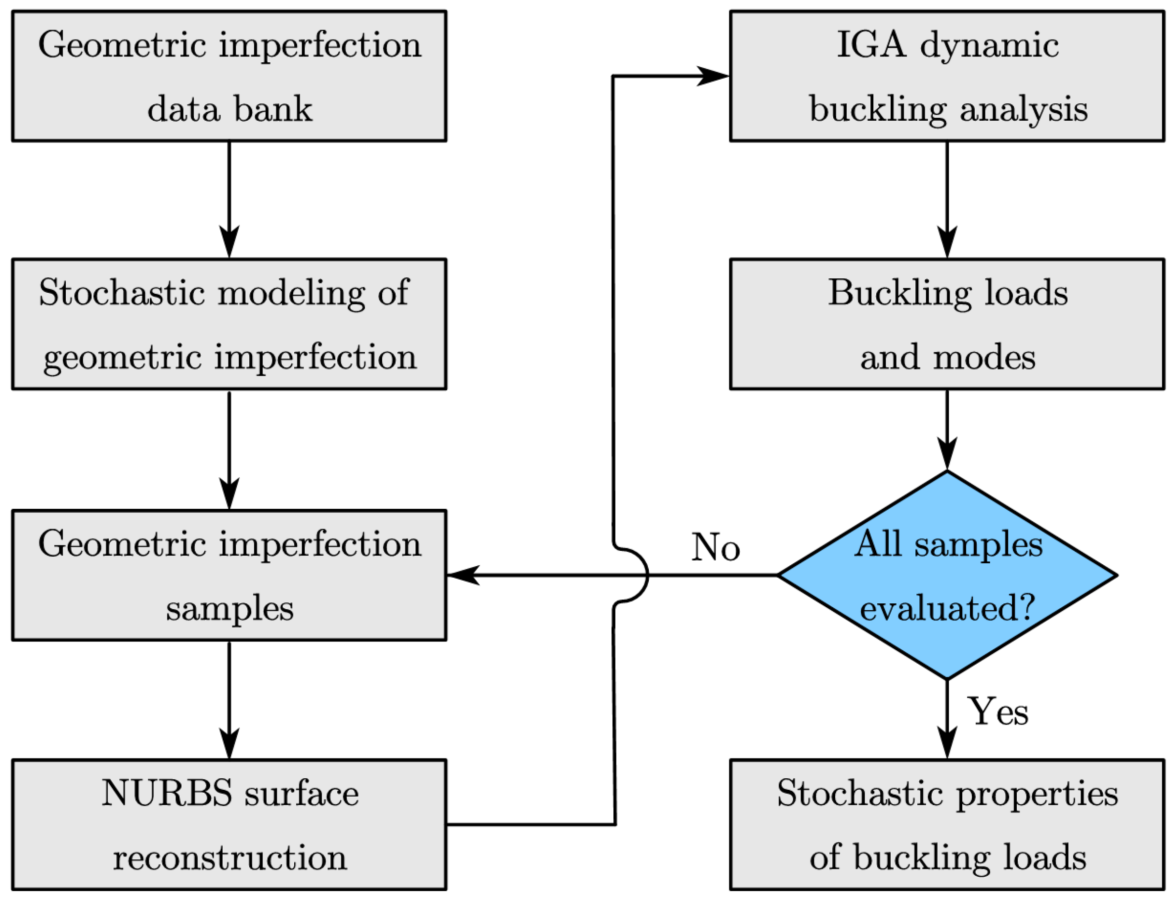
In this paper, we extend our previous work on the buckling analysis of isogeometric shell structures to the stochastic situation. In particular, a deterministic isogeometric dynamic buckling analysis approach combined with a spectral representation of random geometric imperfections is developed to study the stochastic dynamic buckling behaviors of cylindrical shell structures. For deterministic analysis, a modified Generalized-α time integration scheme combined with a nonlinear isogeometric Kirchhoff–Love shell element is used to simulate the buckling and post-buckling problems of cylindrical shell structures. The Generalized-α time integration scheme is second-order accurate and can dissipate high-frequency contents with less influence on the low-frequency contents. Therefore, it is a desirable time integration approach to dynamic buckling analysis. To incorporate the geometric imperfections, an NURBS surface reconstruction method is developed to model the measured geometric imperfection data of the cylindrical shell. Then, the reconstructed model can be naturally incorporated into the isogeometric framework due to the seamless integration of CAD and CAE models inherited in IGA. Additionally, the smooth and high-order continuous geometric representation naturally eliminates the artificial geometric imperfections caused by finite element meshes. This property may improve the prediction accuracy and computational efficiency in dynamic buckling problems. For stochastic analysis, the method of separation is adopted to model the stochastic geometric imperfections of cylindrical shells based on a set of measurements. Then, an arbitrary number of samples can be generated to evaluate the stochastic dynamic buckling behaviors of cylindrical shells. For comparison, the stochastic buckling behaviors of cylindrical shells under static loads are also studied, different features obtained by static and dynamic analysis are highlighted, and suggestions are made for the design of this type of shell structure. To better illustrate the method used in this paper, a flowchart of the proposed approach is shown in Figure 1.
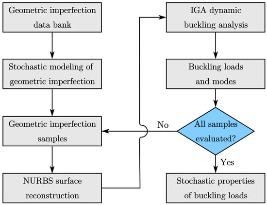
Figure 1.
Flowchart of the methodologies.
This paper is organized as follows. The Kirchhoff–Love shell theory, isogeometric discretizations, and Generalized-α time integration scheme are introduced in Section 2. Then, the stochastic modeling of geometric imperfections is discussed in Section 3. Several numerical examples are presented in Section 4. Finally, we summarize the main findings and draw conclusions in Section 5.
2. Isogeometric Kirchhoff–Love Shell Element
In this section, the fundamental theories governing the dynamic analysis of isogeometric thin-shell structures are presented, which include the Kirchhoff–Love shell kinematics in Section 2.1, the governing equations and isogeometric discretizations in Section 2.2, and the implicit time integration in Section 2.3. We note that the Greek indices in this section take values 1, 2, and the Latin indices take values 1, 2, 3. Additionally, we use uppercase notation for quantities that refer to the undeformed reference configuration, and lowercase notation for quantities that refer to the current deformed configuration.
2.1. Shell Kinematics
The 3D shell body in the undeformed and deformed configurations can be described as follows:
where X and x represent the material point coordinates of the 3D shell body, and represent the material point coordinates on the shell’s mid-surface, and represent the parameterized coordinates of the shell body with . Here, h is the shell thickness. The directors of the shell mid-surface can be calculated as follows:
where and , which can be obtained by differentiating the position vector with respect to the parametric coordinate.
The displacement of the shell mid-surface can be expressed as follows:
According to the Kirchhoff–Love assumption, the transverse normal and shear strains of the shell body can be neglected; therefore, the Green–Lagrange strain tensor E can be simplified as follows:
where is the Green–Lagrange strain tensor coefficients, and and are the membrane and bending strain tensor coefficients, respectively, which can be expressed as follows:
where
where and represent the derivative of and with respect to the parametric coordinate , respectively.
The contravariant base vectors and in Equation (4) relate to the covariant base vectors and with
Assuming the St. Venant–Kirchhoff constitutive model, the membrane force and bending moment resultants relate to the membrane and bending strain components, respectively, as follows:
where the overhead tilde represents the quantities defined in the local Cartesian coordinate system, and C is the reduced material tensor for the plane stress problem, which can be defined as follows:
where E is the Young’s modulus and ν is the Poisson ratio of the material.
2.2. Governing Equations and Isogeometric Discretizations
The governing equations of geometrically nonlinear Kirchhoff–Love shells can be formulated as follows:
where A is the shell mid-surface surface area, P0 is the distributed surface load, T0 is the traction along the Neumann boundary , ρ is the material density, is the acceleration of the shell, N and M are the vector form of the membrane force and bending moment resultants, respectively, and are the vector form of the membrane and bending strain components, respectively, and the symbol δ represents the variation in the quantity.
In isogeometric analysis, the physical field is discretized with the same NURBS basis functions as the geometric descriptions leading to the following formulations:
where n is the total number of basis functions, Ri is the i-th NURBS basis function defined by two parametric coordinates , and Pi is the i-th control point defined by three cartesian coordinates. Then, the geometry of a shell mid-surface can be defined by the summation of each control point multiplied by its corresponding NURBS basis functions, cf. Equation (15). For more details of NURBS basis and geometric descriptions, we refer to [40]. In addition, Ui is the displacement vector of the i-th control point, and R, P, U, and δU in Equations (15)–(17) represent the matrices containing all the corresponding quantities.
Substituting Equations (15)–(17) into Equation (14) and leveraging the arbitrary nature of , the semi-discretized governing equations for the Kirchhoff–Love shell can be obtained:
where f is the external force vector, r is the internal force vector, and Ma is the mass matrix.
2.3. Implicit Time Integration Scheme
The semi-discretized equilibrium Equation (18) can be solved sequentially by an appropriate time discretization scheme. In this paper, we adopt the Generalized-α time marching scheme, which preserves second-order accuracy and has controllable high-frequency numerical dissipation. We assume that the total time span [0, T] of dynamic analysis is partitioned into typical time intervals [tn, tn+1], with the time step size Δt = tn+1 − tn. The physical quantities at the time tn are known, and we would like to solve for the unknown quantities at the time tn+1.
Applying Newmark’s approximation, the acceleration and velocities at the end of the time step tn+1 are formulated as follows:
where β and γ are the integration parameters that determine the characteristics of the system.
For the Generalized-α time integration scheme, the quantities in Equation (18) are evaluated at the general midpoints and within the time interval [tn, tn+1], which leads to the modified governing equations:
where the subscripts in Equation (21) represent time discrete combinations and can be expressed as follows:
The inner force in Equation (21) is evaluated as follows:
where
The parameters , , β, and γ determine the stability and accuracy of the time integration scheme; they can be expressed as follows:
where is the spectral radius that controls the amount of high-frequency numerical dissipation during time integration. For values of , there is no high-frequency dissipation, while for , this corresponds to the case of asymptotic annihilation.
Substituting Equations (19) and (22)–(25) into Equation (21) results in the effective governing equation:
The linearization of the nonlinear residual Equation (27) results in the following:
where the superscripts k and k+1 signify the iteration number in each time step. Substituting Equation (27) into (28) results in the following:
where is the displacement increment at the (k + 1)-th iteration. Equation (29) can then be solved iteratively with the Newton–Raphson method within each time step.
The effective stiffness matrix in Equation (29) can be written as follows:
where is the tangent stiffness matrix, formulated as follows:
3. Stochastic Modeling of Geometric Imperfections
The geometric imperfections of cylindrical shell structures can be viewed as a univariate two-dimensional (1V-2D) non-stationary stochastic process, where the deviation between the shell mid-surface and the radius of the perfect cylinder is taken as the random variable. To estimate the characteristics of the geometric imperfection random field, the spectral representation method is used in this paper to obtain the power spectral density function. Based on the established random field description, an arbitrary number of samples can be generated for the subsequent Monte Carlo simulation. In the following section, we describe the basic procedure of random field modeling with the spectral representation method.
According to the spectral representation method, the geometric imperfection samples of the shell structure can be described as follows:
where the superscript r represents the r-th realization, x1 and x2 are the physical coordinates of the random field, and
where and are the cut-off frequencies, beyond which the power spectra are assumed to be zero, N1 and N2 determine the discretization of the active frequency range, and in Equation (32) are the random phase angels uniformly distributed in the range , and is the power spectrum of the geometric random field, which needs to be estimated based on the data for imperfection measurements.
For a narrow-banded power spectrum, typical in geometric imperfections, we assume that the frequency and spatial contents of the spectrum are separable, which leads to the following multiplicative simplification of the power spectrum:
where is the spectral density function, and is the modulating envelope.
The homogeneous Fourier power spectrum can be estimated as follows:
where the overhead hat represents the corresponding estimation of the quantity, are the available realizations of the stochastic field, and L1 and L2 are the two dimensions of the physical domain. For rectangular random fields, these represent the length and width of the physical domain, respectively. Basically, Equation (37) averages the frequency content of the separable input samples over their length by Fourier transformation.
The estimation of the modulating envelope can be derived from the mean square of samples as follows:
The final estimate of the spectrum Equation (36) can now be established by replacing and with their estimates and :
The discrete Fourier transform of strongly narrow-band functions is sensitive to leakage errors due to the limited number of discrete frequency points. Therefore, a Hamming window can be applied prior to the application of the Fourier transformation, with the Hamming window defined as follows:
where for the length direction, T = L1, and for the width direction, T = L2.
Then, the estimated power spectrum Equation (37) can be modified as follows:
4. Numerical Examples
In this section, we first illustrate the accuracy of the proposed isogeometric dynamic buckling analysis with a cylindrical shell example where measured geometric imperfections are considered. Then, we estimate the random field of the geometric imperfections for the cylindrical shell based on a set of measured imperfection data. Finally, the stochastic characteristics of the buckling loads are evaluated based on 500 realizations of the cylindrical shell.
4.1. Dynamic Buckling of Cylindrical Shell with Measured Geometric Imperfections
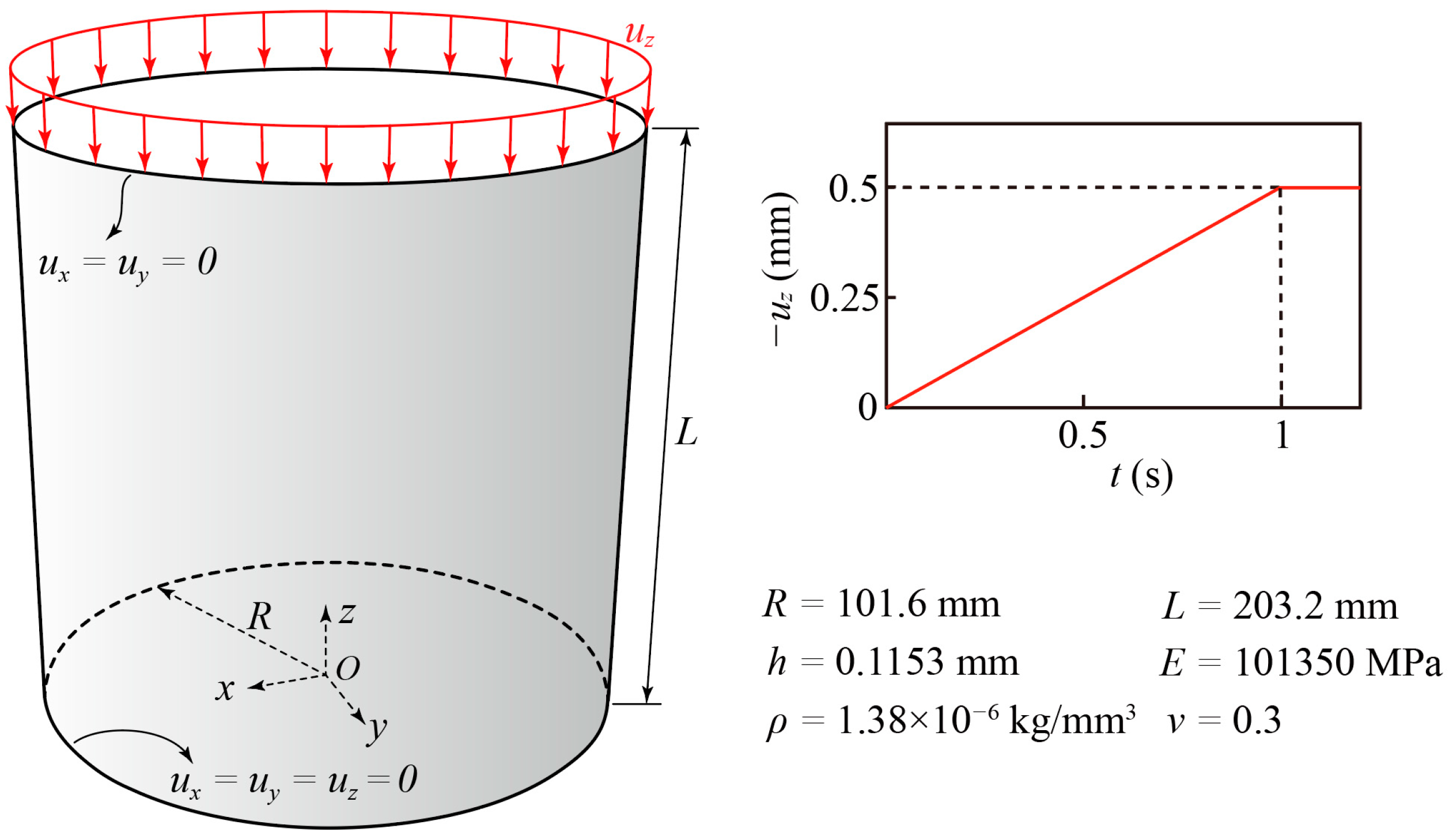
In this example, a cylindrical shell denoted as A9 with measured geometric imperfections is considered to test the accuracy of the proposed isogeometric method for dynamic buckling analysis. The geometric descriptions and material properties are shown in Figure 2. The upper and lower rims of the cylindrical shell are simply supported, except that the upper rim is subjected to a vertical displacement boundary condition with the velocity equal to 0.5mm/s. The boundary conditions can be expressed as follows:
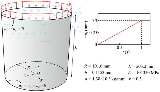
Figure 2.
Cylindrical shell A9 with measured geometric imperfections: geometric and boundary conditions and material properties.
The geometric imperfection data for the cylinder A9 are taken from the imperfection data bank of TU Delft [41], where a series of 2D Fourier coefficients are provided to represent the deviations of the shell surface with respect to the perfect cylinder. The half-wave cosine representation of the geometric imperfections is expressed as follows:
where and are the axial and circumferential coordinates of the cylinder, k and l are the axial and circumferential half-wave numbers, respectively, and Akl and Bkl are the harmonic components, which can be found in the reference [12]. The imperfection field can be added to the perfect cylinder to generate the real geometries of the cylinder.
In order to construct the geometric imperfect shell model for isogeometric analysis, a set of 101 × 301 uniform grid sampling points, , are generated based on the imperfection field of Equation (43), where and are the axial and circumferential coordinates of the sampling points. Then, the generated imperfection values are added to the radius R of the cylindrical shell, and the physical coordinates of each sampling points can be calculated as follows:
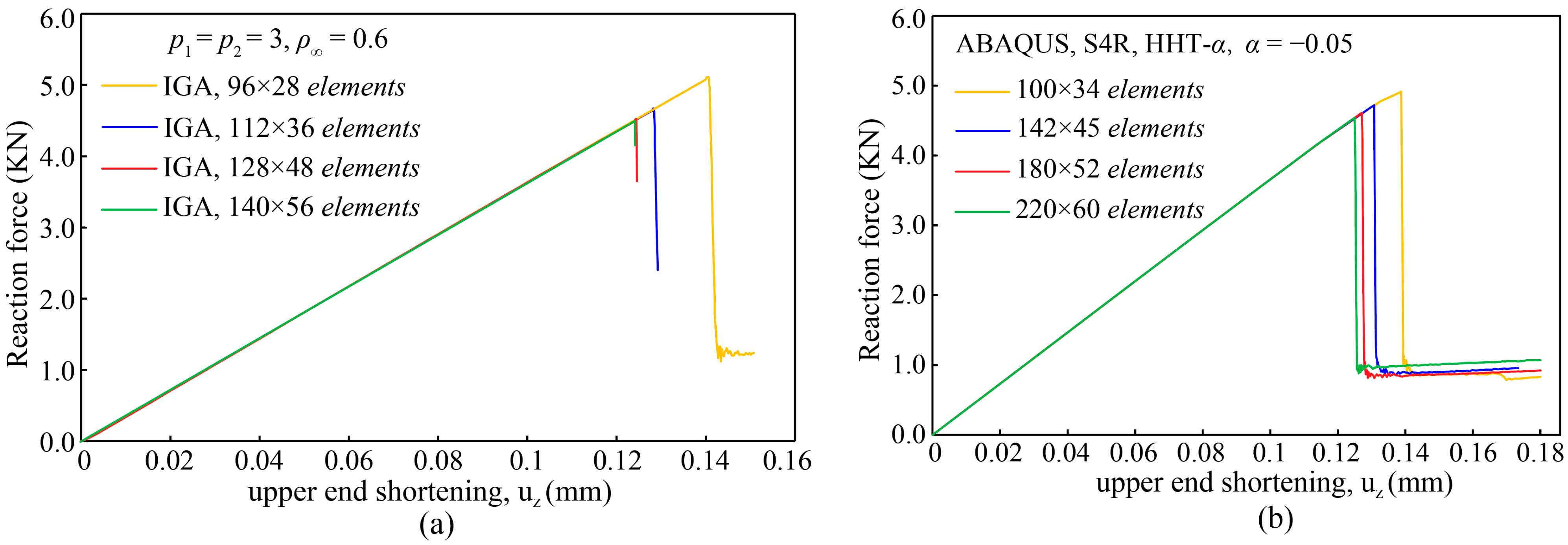
Then, a set of orthogonal NURBS curves are constructed by interpolating the grid points, , based on which the NURBS surface can be generated in CAD software Rhinoceros 5 [42]. In order to study the convergence properties of the isogeometric model, we discretize the shell with 96 × 28, 112 × 36, 128 × 48, and 140 × 56 NURBS elements with the order of the basis p = q = 3. For comparison, a finite element solution was generated based on ABAQUS software [43], with 13,200 S4R shell elements used.
Figure 3 shows the convergence study of the dynamic buckling analysis of the A9 shell with IGA and ABAQUS. It can be observed that the IGA model predicts a buckling load of 4522.5 N with a mesh of 128 × 48 elements, while, for the ABAQUS model, it is difficult to obtain a converged value for dynamic buckling, even with a relatively fine mesh of 220 × 60 elements, which demonstrates the deficiency of the linear facet elements of FEM in approximating real, complex geometric imperfection shapes. This observation signifies the importance of geometric imperfection modeling in shell buckling analysis and shows the superior properties of IGA in which smooth and high-order continuous geometric representations are naturally incorporated. The dynamic buckling load predicted by ABAQUS with a mesh of 220 × 60 elements is 4540.1 N, which is very close to the results of the IGA model. The theoretical buckling load for cylindrical shell can be calculated as follows [44]:
which is 5123.7 N for shell A9. Equation (45) is suitable for a very thin cylindrical shell with a length L not smaller than the diameter. Additionally, the static buckling load obtained with a nonlinear isogeometric shell element and arc-length path-following method is 4379 N [12], which is smaller than the corresponding dynamic buckling loads. This phenomenon reflects the effects of inertial force on the stability properties of cylindrical shells.
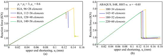
Figure 3.
Cylindrical shell A9 with measured geometric imperfections: (a) convergence of IGA model, (b) convergence of ABAQUS model.
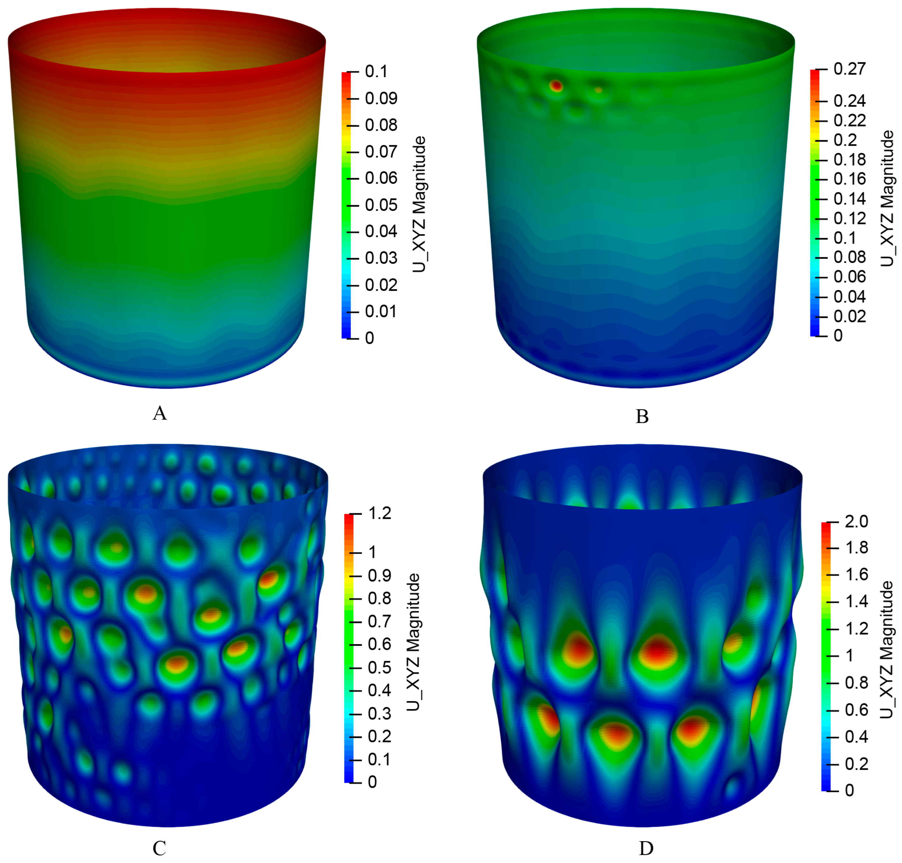
Figure 4 shows the contour plots of the cylindrical shell A9 during dynamic buckling analysis. It can be observed that the buckling initiates at the local dimple near the upper rim of the shell. Then, the buckling spreads out through the whole shell surface and finally reaches a relatively stable buckling mode with 2 and 13 half waves in the axial and circumferential directions, respectively.
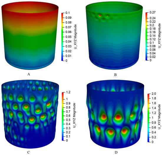
Figure 4.
Contour plots of the cylindrical shell A9 during dynamic buckling analysis: (A) pre-buckling state, (B) initial buckling state, (C) post-buckling transition state, (D) post-buckling stable state.
4.2. Stochastic Buckling Analysis of a Cylindrical Shell
In this example, the stochastic buckling analysis of a cylindrical shell is studied, with the same geometric and material properties as in the example of Section 4.1 being adopted. Seven cylindrical shells with measured geometric imperfections, , are taken from the geometric imperfection data bank of TU Delft [41]. The geometric imperfection data of the seven cylindrical shells are stored as Fourier coefficients Akl and Bkl, the same as in Equation (43).
For the estimation of the geometric imperfection random field, we first determine the mean function of the measured imperfections . Then, a zero-mean ensemble of samples can be obtained as , which can be used for the estimation of the spectrum and spatial envelope. The cut-off frequencies are set to be , and the number of discrete frequencies in two directions are set to be N1 = N2 = 100.
The mean square function and the normalized homogeneous spectrum of the cylindrical shell samples are shown in Figure 5 and Figure 6, respectively.
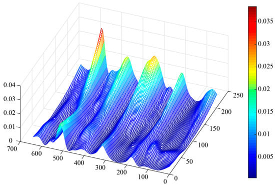
Figure 5.
Mean square function determined from measurements of cylindrical shells.
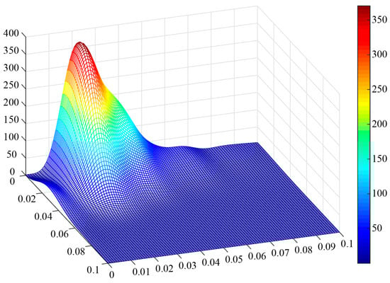
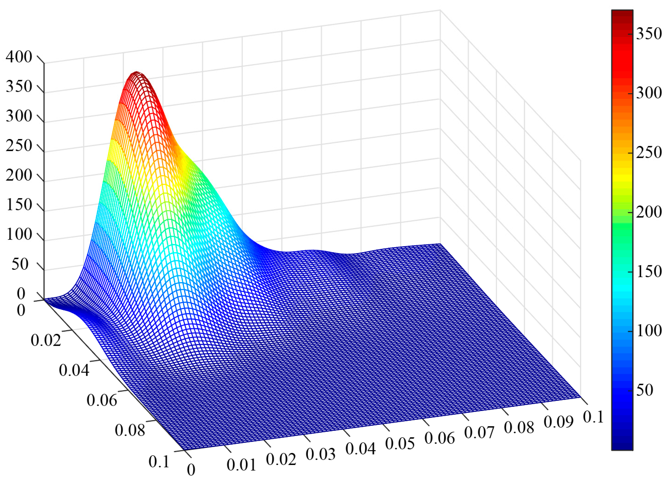
Figure 6.
Normalized homogeneous spectrum with Hamming window.
Based on the estimated spectrum, an arbitrary number R of random imperfection samples can be generated; see Figure 7 for one of the imperfection samples. To simulate the original non-zero mean process, the mean function needs to be superposed to the zero-mean ensemble of simulations, as follows:
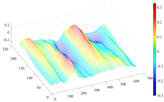
Figure 7.
Sample of the generated geometric imperfection field.
Using the above geometric imperfection realizations, the corresponding isogeometric shell models are generated based on NURBS surface fitting in Rhino. Then, the dynamic buckling behaviors, such as buckling loads and modes for each shell, are simulated by deterministic isogeometric dynamic buckling analysis. After all of the shell samples are analyzed, the buckling load and failure variabilities of the cylindrical shell can be evaluated.
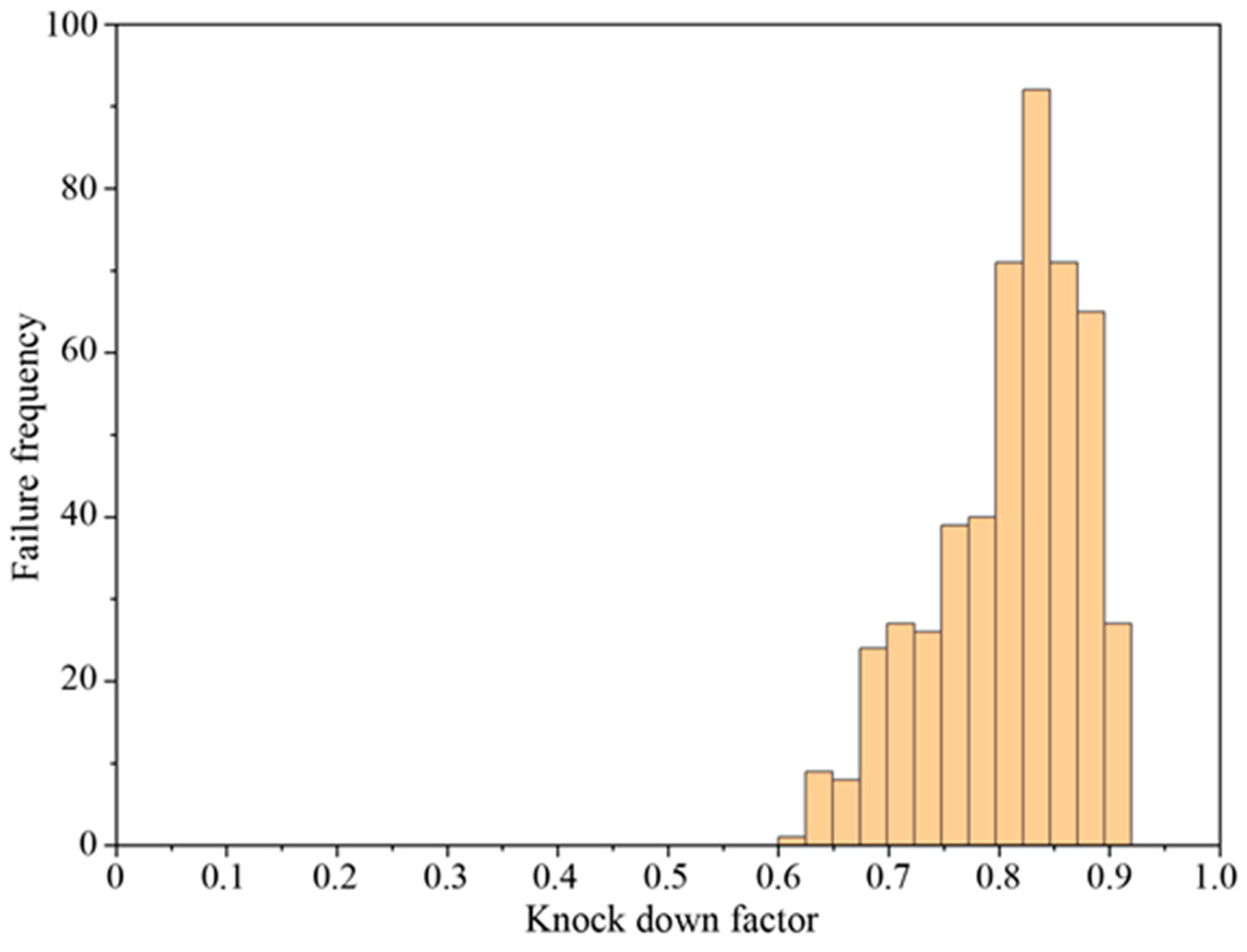
In this example, 500 geometric imperfection samples are generated and the corresponding shell models are simulated based on the proposed isogeometric dynamic buckling analysis framework. The boundary conditions are the same as in the example in Section 4.1. The buckling load variability of the cylindrical shell under dynamic load is shown in Figure 8, where the mean value of the knock down factor is 0.809, and the coefficient of variation is 8.2%. For comparison, the buckling load variability obtained with static nonlinear arc-length method is shown in Figure 9, where the mean value of the buckling load knock down factor is 0.782 and the coefficient of variation is 9.4%. We note that the knock down factor is the buckling load normalized with respect to the theoretical buckling load of the cylindrical shell; see Equation (45). It can be observed from Figure 8 and Figure 9 that the mean value for the buckling load obtained with dynamic analysis is slightly higher than with static nonlinear analysis, which might be due to the dynamic effects of the applied impulse load. Moreover, the variability in the dynamic buckling load is smaller than the static buckling load, which means that the dispersion degree of dynamic buckling loads is lower than the static case. This observation signifies that the cylindrical shell structures are less sensitive to variations in the geometric imperfections in the dynamic situation, which might be caused by the interaction between the geometric imperfection and the vibration modes.

Figure 8.
Buckling load distributions for cylindrical shells, obtained through the isogeometric dynamic buckling analysis of 500 shell samples.
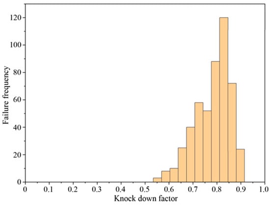
Figure 9.
Buckling load distributions for cylindrical shells, obtained via isogeometric nonlinear static buckling analysis of 500 shell samples.
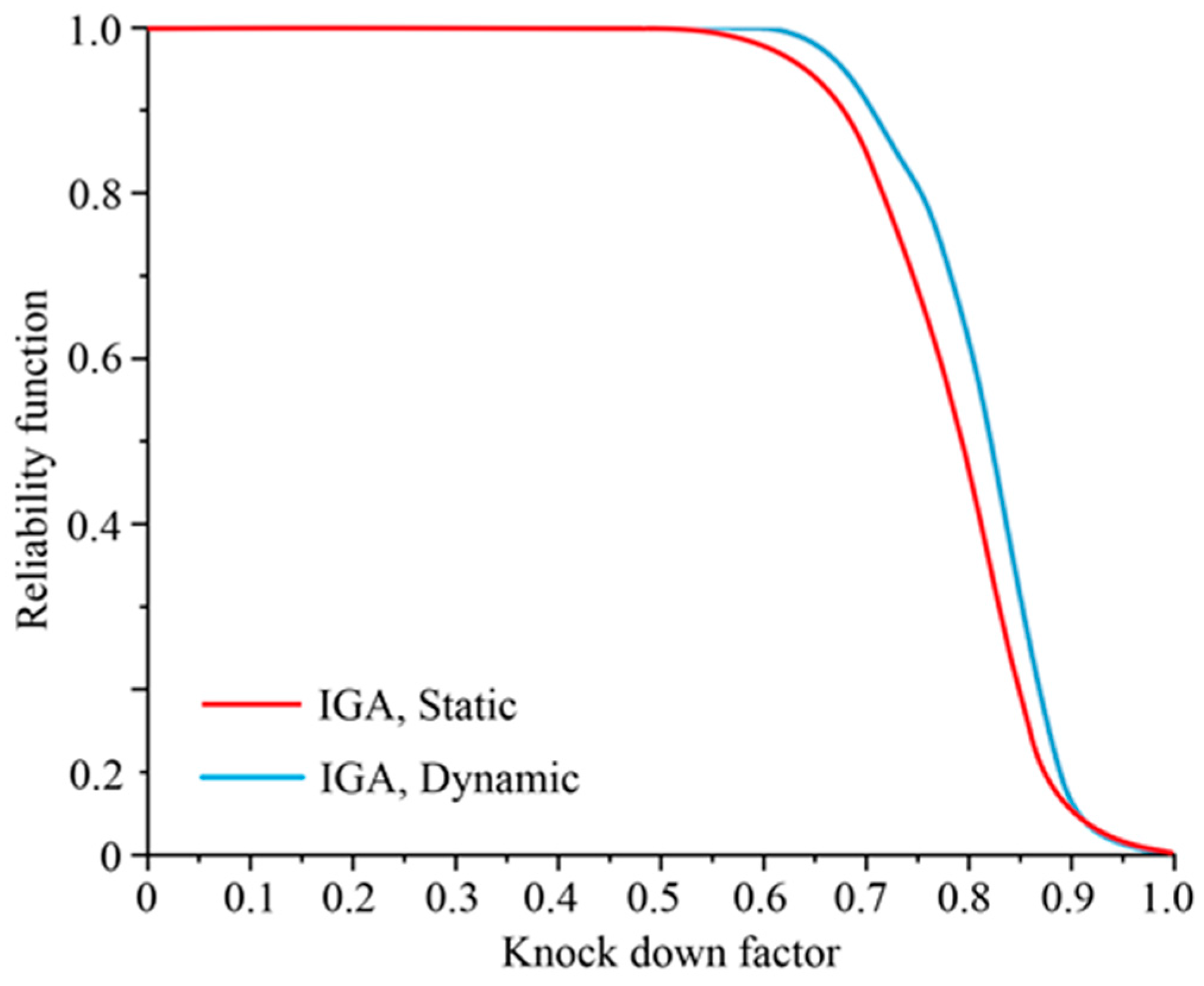
Figure 10 shows the reliability functions of the knock down factor for both dynamic and static buckling analysis. This can be used to design cylindrical shell structures under buckling constraints with a desired level of confidence. The reliability of the shell structure under a buckling situation will decrease when the designed buckling load increases. Moreover, this also shows that the reliability of the cylindrical shell under a dynamic buckling load is slightly higher than that under a static buckling load. The above observations suggest potential improvements in designing cylindrical shell structures under dynamic loads.
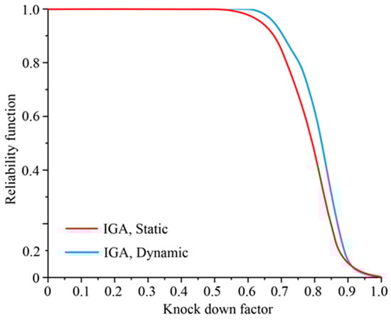
Figure 10.
Reliability curves for cylindrical shell structures for static and dynamic buckling analysis.
5. Conclusions
In this paper, we extend our previous work on the dynamic buckling analysis of isogeometric shell structures to a stochastic situation where a deterministic buckling analysis method combined with a spectral-based stochastic model of geometric imperfections is adopted. For deterministic analysis, a modified Generalized-α time integration scheme combined with a nonlinear isogeometric Kirchhoff–Love shell element is used to simulate buckling and post-buckling problems in cylindrical shell structures. In particular, geometric imperfections are constructed based on NURBS surface fitting and incorporated into the isogeometric analysis framework seamlessly. For stochastic analysis, the method of separation is adopted to model the stochastic geometric imperfections of cylindrical shells based on a set of measurements.
We tested the accuracy of the proposed method with a cylindrical shell example, where measured geometric imperfections were incorporated. It was found that the isogeometric method shows superior convergence properties and can capture geometric imperfections more accurately than the ABAQUS FEM reference solutions. It is shown that ABAQUS solutions show extreme mesh sensitivity, and is difficult to obtain a converged dynamic buckling load even with a very fine mesh. This phenomenon signifies the deficiency of linear facet elements used to represent a complex geometric imperfection field, while, for the isogeometric method, the reconstructed geometry of the cylindrical shell is smooth and high-order continuous, which naturally eliminates the artificial geometric imperfections of FE mesh.
For stochastic dynamic buckling analysis, 500 samples of cylindrical shells are generated based on seven nominally identical shells reported in the geometric imperfection data bank. Then, the buckling load variability is obtained by deterministic buckling analysis of the generated shell samples. It is found that the average value of buckling loads obtained by dynamic analysis is slightly higher than those from nonlinear static stochastic buckling analysis, which might be due to the dynamic effects of the applied impulse load. Moreover, the coefficient of variation for the dynamic buckling load is lower than for the static one, which shows that, in a dynamic situation, the dispersion degree of the buckling load is lower than the static case, although the imperfect cylindrical shell samples adopted are the same. This observation signifies that the cylindrical shell structures are less sensitive to the variations in the geometric imperfections in the dynamic situation, which might be caused by the interaction between the geometric imperfection and the vibration modes. In addition, the reliability functions of the cylindrical shells under static and dynamic loads are also studied and suggest that potential improvements can be achieved in designing cylindrical shell structures under dynamic loads considering the same reliability.
For future research, the stochastic characteristics of the cylindrical shell subject to different dynamic loading cases could be studied. Additionally, we can also extend our framework to the composite shell structures and stiffened shell structures that are widely used in aircraft fuselages and rocket bodies.
Author Contributions
Conceptualization, Y.G.; methodology, Q.Y.; software, F.X.; validation, Q.Y. and Z.G.; investigation, Q.Y. and F.X.; writing—original draft preparation, Q.Y. and Z.G.; writing—review and editing, X.L.; funding acquisition, Y.G. and J.Z. All authors have read and agreed to the published version of the manuscript.
Funding
This research was funded by THE NATIONAL KEY LABORATORY OF STRENGTH AND STRUCTURAL INTEGRITY, grant number LSSIKFJJ202403014, and SCIENCE AND TECHNOLOGY MAJOR SPECIAL PROJECT OF SHANXI PROVINCE, grant number 202101120401007.
Data Availability Statement
The data presented in this study are available on request from the corresponding authors.
Conflicts of Interest
The authors declare no conflicts of interest.
References
- Arbocz, J.; Babcock, C.D., Jr. The effect of general imperfections on the buckling of cylindrical shells. J. Appl. Mech. 1969, 36, 28–38. [Google Scholar] [CrossRef]
- Papadopoulos, V.; Stefanou, G.; Papadrakakis, M. Buckling analysis of imperfect shells with stochastic non-gaussian material and thickness properties. Int. J. Solids Struct. 2009, 46, 2800–2808. [Google Scholar] [CrossRef]
- Simitses, G. Buckling and postbuckling of imperfect cylindrical shells: A review. Appl. Mech. Rev. 1986, 39, 1517–1524. [Google Scholar] [CrossRef]
- Arbocz, J.; Starnes, J.H., Jr. Future directions and challenges in shell stability analysis. Thin Walled Struct. 2002, 40, 729–754. [Google Scholar] [CrossRef]
- Elishakoff, I. Uncertain buckling: Its past, present and future. Int. J. Solids Struct. 2000, 37, 6869–6889. [Google Scholar] [CrossRef]
- DESICOS—New Robust Design Guidelines for Imperfection Sensitive Composite Launcher Structures. Available online: https://cordis.europa.eu/project/rcn/102054/factsheet/en (accessed on 18 July 2024).
- Bisagni, C. Dynamic buckling of fiber composite shells under impulsive axial compression. Thin Walled Struct. 2005, 43, 499–514. [Google Scholar] [CrossRef]
- Less, H.; Abramovich, H. Dynamic buckling of a laminated composite stringer-stiffened cylindrical panel. Compos. Part B 2012, 43, 2348–2358. [Google Scholar] [CrossRef]
- Ari-Gur, J.; Simonetta, S. Dynamic pulse buckling of rectangular composite plates. Compos. Part B Eng. 1997, 28, 301–308. [Google Scholar] [CrossRef]
- Ghannadi, P.; Kourehli, S.; Nguyen, A. The differential evolution algorithm—An analysis of more than two decades of application in structural damage detection (2001–2022). In Data Driven Methods for Civil Structural Health Monitoring and Resilience; CRC Press: Boca Raton, FL, USA, 2024. [Google Scholar]
- Hughes, T.; Cottrell, J.; Bazilevs, Y. Isogeometric analysis: CAD, finite elements, NURBS, exact geometry and mesh refinement. Comput. Meth. Appl. Mech. Eng. 2005, 194, 4135–4195. [Google Scholar] [CrossRef]
- Guo, Y.; Do, H.; Ruess, M. Isogeometric stability analysis of thin shells: Fromsimple geometries to engineering models. Int. J. Numer. Methods Eng. 2019, 118, 433–458. [Google Scholar] [CrossRef]
- Oesterle, B.; Geiger, F.; Forster, D.; Frohlich, M.; Bischoff, M. A study on the approximation power of NURBS and the significance of exact geometry in isogeometric pre-buckling analysis of shells. Comput. Meth. Appl. Mech. Eng. 2022, 397, 115–144. [Google Scholar] [CrossRef]
- Liang, K.; Ruess, M.; Abdalla, M. The Koiter-Netwon approach using von Kármán kinematics for buckling analyses of imperfection sensitive structures. Comput. Meth. Appl. Mech. Eng. 2014, 279, 440–468. [Google Scholar] [CrossRef]
- Hao, P.; Wang, Y.; Tang, H.; Feng, S.; Wang, B. A NURBS-based degenerated stiffener element for isogeometric static and buckling analysis. Comput. Meth. Appl. Mech. Eng. 2022, 398, 115245. [Google Scholar] [CrossRef]
- Magisano, D.; Leonetti, L.; Garcea, G. Unconditional stability in large deformation dynamic analysis of elastic structures with arbitrary nonlinear strain measure and multi-body coupling. Comput. Meth. Appl. Mech. Eng. 2022, 393, 114776. [Google Scholar] [CrossRef]
- Guo, Y.; Pan, M.; Wei, X.; Luo, F.; Sun, F.; Ruess, M. Implicit dynamic buckling analysis of thin-shell isogeometric structures considering geometric imperfections. Int. J. Numer. Methods Eng. 2023, 124, 1055–1088. [Google Scholar] [CrossRef]
- Guo, Y.; Chen, Z.; Wei, X.; Hong, Z. Isogeometric dynamic buckling analysis of trimmed and multipatch thin-shell structures. AIAA J. 2023, 61, 5620–5634. [Google Scholar] [CrossRef]
- Leidinger, L.F.; Breitenberger, M.; Bauer, A.M.; Hartmann, S.; Wüchner, R.; Bletzinger, K.U.; Duddeck, F.; Song, L. Explicit dynamic isogeometric B-Rep analysis of penalty-coupled trimmed NURBS shells. Comput. Meth. Appl. Mech. Eng. 2019, 351, 891–927. [Google Scholar] [CrossRef]
- Lavrenčič, M.; Brank, B. Simulation of shell buckling by implicit dynamics and numerically dissipative schemes. Thin Walled Struct. 2018, 132, 682–699. [Google Scholar] [CrossRef]
- Newmark, N. A method of computation for structural dynamics. ASCE J. Eng. Mech. Div 1959, 85, 67–94. [Google Scholar] [CrossRef]
- Chung, J.; Hulbert, G. A time integration algorithm for structural dynamics with improved numerical dissipation—The generalized-α method. J. Appl. Mech. 1993, 60, 371–375. [Google Scholar] [CrossRef]
- Kuhl, D.; Crisfield, M. Energy conserving and decaying algorithms in non-linear structural dynamics. Int. J. Numer. Methods Eng. 1999, 45, 569–599. [Google Scholar] [CrossRef]
- Kuhl, D.; Ramm, E. Generalized Energy-Momentum Method for non-linear adaptive shell dynamics. Comput. Meth. Appl. Mech. Eng. 1999, 178, 343–366. [Google Scholar] [CrossRef]
- Stefanou, G. The stochastic finite element method: Past, present and future. Comput. Meth. Appl. Mech. Eng. 2009, 198, 1031–1051. [Google Scholar] [CrossRef]
- Schenk, C.A.; Schuëller, G.I. Buckling analysis of cylindrical shells with cutouts including random boundary and geometric imperfections. Comput. Meth. Appl. Mech. Eng. 2005, 196, 3424–3434. [Google Scholar] [CrossRef]
- Schillinger, D.; Stefanov, D.; Stavrev, A. The method of separation for evolutionary spectral density estimation of multi-variate and multi-dimensional non-stationary stochastic process. Probablistic Eng. Mech. 2013, 33, 58–78. [Google Scholar] [CrossRef]
- Schillinger, D.; Papadopoulos, V. Accurate estimation of evolutionary power spectra for strongly narrow-band random fields. Comput. Meth. Appl. Mech. Eng. 2010, 199, 947–960. [Google Scholar] [CrossRef]
- Ghanem, R.; Spanos, P.D. Stochastic Finite Elements: A Spectral Approach; Dover: Mineola, NY, USA, 2003. [Google Scholar]
- Stefanou, G.; Papadrakakis, M. Assessment of spectral representation and Karhunen-Loeve expansion methods for the simulation of Gaussian stochastic fields. Comput. Meth. Appl. Mech. Eng. 2007, 196, 2465–2477. [Google Scholar] [CrossRef]
- Shinozuka, M.; Deodatis, G. Simulation of stochastic process by spectral representation. ASME Appl. Mech. Rev 1991, 44, 191–203. [Google Scholar] [CrossRef]
- Grigoriu, M. On the spectral representation method in simulation. Probabilistic Eng. Mech. 1993, 8, 75–90. [Google Scholar] [CrossRef]
- Vanmarcke, E.H. Random Fields: Analysis and Synthesis; Academic Press: London, UK, 1983. [Google Scholar]
- Deodatis, G. Non-stationary stochastic vector process: Seismic ground motion applications. Probabilistic Eng. Mech. 1996, 11, 149–167. [Google Scholar] [CrossRef]
- Deodatis, G.; Schinozuka, M. Auto-regressive model for non-stationary stochastic processes. ASCE J. Eng. Mech 1988, 114, 1995–2012. [Google Scholar] [CrossRef]
- Carmona, R.; Hwang, W.J.; Torrésani, B. Practical Time-Frequency Analysis; Academic Press: New York, NY, USA, 1998. [Google Scholar]
- Newland, D.E. An Introduction to Random Vibrations, Spectral and Wavelet Analysis; Wiley: New York, NY, USA, 1993. [Google Scholar]
- Stavrev, A.; Stefanov, D.; Schillinger, D.; Rank, E. Comparison of eigenmode based and random field based imperfection modeling for the stochastic buckling analysis of I-section beam-columns. Int. J. Struct. Stab. Dyn. 2013, 13, 1350021. [Google Scholar] [CrossRef]
- Broggi, M.; Schuëller, G.I. Efficient modeling of imperfections for buckling analysis of composite cylindrical shells. Eng. Struct. 2011, 33, 1796–1806. [Google Scholar] [CrossRef]
- Piegl, L.; Tiller, W. The NURBS Book—Monographs in Visual Communication; Springer: Berlin/Heidelberg, Germany, 1997. [Google Scholar]
- Arbocz, J.; Abramovich, H. The Initial Imperfection Data Bank at the Delft University of Technology, Part I; Technical Report LR-290; Delft University of Technology: Delft, The Netherlands, 1979. [Google Scholar]
- Rhinoceros—NURBS Modeling for Windows. Available online: http://www.rhino3d.com (accessed on 29 August 2024).
- ABAQUS/Standard Analysis User’s Manual. Available online: http://130.149.89.49:2080/v2016/index.html (accessed on 29 August 2024).
- Timoshenko, S.; Gere, J. Theory of Elastic Stability; McGraw Hill: Singapore, 1985. [Google Scholar]


Disclaimer/Publisher’s Note: The statements, opinions and data contained in all publications are solely those of the individual author(s) and contributor(s) and not of MDPI and/or the editor(s). MDPI and/or the editor(s) disclaim responsibility for any injury to people or property resulting from any ideas, methods, instructions or products referred to in the content. |
© 2024 by the authors. Licensee MDPI, Basel, Switzerland. This article is an open access article distributed under the terms and conditions of the Creative Commons Attribution (CC BY) license (https://creativecommons.org/licenses/by/4.0/).