Abstract
The application of contrastive learning in image clustering in the field of unsupervised learning has attracted much attention due to its ability to effectively improve clustering performance. Extracting features for face-oriented clustering using deep learning networks has also become one of the key challenges in this field. Some current research focuses on learning valuable semantic features using contrastive learning strategies to accomplish cluster allocation in the feature space. However, some studies decoupled the two phases of feature extraction and clustering are prone to error transfer, on the other hand, features learned in the feature extraction phase of multi-stage training are not guaranteed to be suitable for the clustering task. To address these challenges, We propose an end-to-end multi-branch feature fusion comparison deep clustering method (SwEAC), which incorporates a multi-branch feature extraction strategy in the representation learning phase, this method completes the clustering center comparison between multiple views and then assigns clusters to the extracted features. In order to extract higher-level semantic features, a multi-branch structure is used to learn multi-dimensional spatial channel dimension information and weighted receptive-field spatial features, achieving cross-dimensional information exchange of multi-branch sub-features. Meanwhile, we jointly optimize unsupervised contrastive representation learning and clustering in an end-to-end architecture to obtain semantic features for clustering that are more suitable for clustering tasks. Experimental results show that our model achieves good clustering performance on three popular image datasets evaluated by three unsupervised evaluation metrics, which proves the effectiveness of end-to-end multi-branch feature fusion comparison deep clustering methods.
MSC:
68T07
1. Introduction
Handling labeled data has been a longstanding issue in the field of machine learning, but real-world data tend to be unlabelled and massive. As the field of deep learning and data mining grows and develops, clustering shows great potential in the field of unlabeled data. Clustering, as an unsupervised learning method, can capture the consistency and relative differences between data from a large amount of unlabeled data. K-means clustering [1] and spectral clustering [2] are common methods in the field of clustering. They are prone to problems such as the “Curse of Dimensionality” and inaccurate clustering results when facing large, high-dimensional data sets. Traditional clustering is limited due to the feature representation of the data, and it has poor scalability. To alleviate this problem, deep clustering decouples the feature representation and clustering of high-dimensional data while obtaining low-dimensional feature representations by nonlinearly mapping an image to the latent space through a deep learning network [3].
Deep clustering utilizes deep neural networks to mine the non-linear features of high-dimensional data, demonstrating powerful non-linear mapping capabilities. In order to more efficiently obtain feature spaces that can easily be clustered and grouped, architectures such as self-encoders [1], comparative learning [4,5], and generative adversarial networks [6,7] are commonly used to efficiently capture feature distributions in the latent space. Currently, staged model training for decoupled representation learning and clustering tasks is commonly used as a training strategy [8], during which errors in the previous stage are easily transferred to the next stage in multi-stage-separation task training. Feature extraction and clustering have also been combined into a unified end-to-end architecture as a training strategy [9,10]. Representation learning is used as a prior for the clustering task to update the network alternately and iteratively during training with a global perspective.
Deep-contrast clustering uses comparative learning to extract higher-order features in order to perform an unsupervised clustering task based on the extracted feature representations [8,11]. Comparative learning compares positive and negative samples in the data space to measure the similarity between target samples. Due to the semantic consistency of the positive sample pairs, higher-order features of the data are learned by bringing the positive sample pairs closer together and distancing the negative samples [12,13]. An encoder is commonly used to learn feature vectors in comparative learning. Due to the limitation of the scanning range of the convolutional sensory field and the use of the same convolutional kernel parameters, the sensibility for higher-level semantic features is somewhat limited. There is also a neglect of location information, as well as the importance of individual features, which is limited due to the identification of salient features, thus affecting clustering performance. In addition to improving the ability to represent features in the potential feature space, learning a clustering-oriented feature representation is likewise advantageous in cluster assignment. In order to jointly address feature representation, as well as clustering assignments for contrast learning, SCAN [8] and DEC [14]) both decouple contrast-feature extraction and clustering, thus completing training in stages. However, due to the coupling between its multiple phases, the learned features may not be guaranteed to fit the clustering task, which in turn may impair the clustering assignment. In order to get better clustering results, it is often necessary to learn a clustering-oriented representation.
In order to overcome the error transfer that occurs in multi-stage tasks and learn better clustering-oriented feature representation, we propose an end-to-end, multi-branch, feature-fusion deep clustering method (SwEAC). We encapsulate comparative representation learning and target clustering in a unified architecture. Specifically, utilizing an unsupervised contrastive learning strategy to identify high-dimensional representations, the network integrates our proposed new multi-branch feature aggregation module EAR to recognize multi-dimensional information. Subsequently, contrasting instance samples are completed using clustering centers, and finally, unsupervised contrastive representation learning and clustering are jointly optimized. The multi-branch feature aggregation module partitions spatial sub-features into multiple groups, utilizing three branches to identify spatial channel features and weighted receptive field spatial features from different dimensions. By merging multi-dimensional information, short-term and long-term dependency relationships are established. Multi-branch feature aggregation can enhance the feature representation capability of convolutional networks, yielding higher-level spatial semantic features. Our main contributions are as follows:
- Proposed a new, end-to-end, multi-branch, feature fusion-comparison deep clustering method. Contrast learning is utilized to accomplish a priori representation learning while fusing aggregated information under multiple branches in a feature extraction network. The contrastive representation-learning stage uses clustering centers to compare instance samples and extract semantically meaningful feature representations. Combined representation learning and clustering for joint training and iterative optimization.
- Designed a new, multi-branch feature-aggregation method. Divided multi-channel sub-features, using a three-branch structure to learn multi-dimensional spatial channel-dimension information and weighted receptive-field spatial features. Completed multi-branch and cross-dimensional information exchange, achieving the aggregation of sub-features and establishing long-term and short-term dependence.
- Designed a clustering-oriented contrastive representation learning strategy. Joint optimization of unsupervised contrastive representation learning and clustering to improve the problem of error transmission faced by multi-stage deep clustering tasks. The training of the model extracts clustering-oriented feature representations in continuous iterations, thus improving the model’s ability to cluster.
Experimental evaluation shows that SwEAC outperforms previous work on several common image clustering datasets. We conducted comparison experiments and ablation experiments on three datasets (CIFAR-10, CIFAR-100/20, and STL10, respectively) to demonstrate the effectiveness of our proposed model.
2. Related Work
Contrastive learning has now become an important branch in the field of unsupervised learning. Its essence lies in using an agent task as a guiding principle for constructing similarities between instances, as well as using an objective function as a supervisory signal for self-supervised learning to guide the learning direction of the model. Early InstDisc [15] proposed individual discrimination as an agent task in conjunction with NCE loss for contrastive learning. CPC [16] used generative agent tasks for training in contrastive learning. With the continuous development of contrastive learning, contrastive-learning architectures generally tend to use the InfoNCE loss function as a supervised signal to guide training, maximizing the mutual information between the whole and the parts. The difference is that MOCO [12] uses an instance-discrimination agent task and proposes the use of a data-structure queue in the dictionary, thus overcoming the problem of negative sample storage size. SimCLR [4] introduces data augmentation to enhance the learning of positive and negative sample pairs through data augmentation. SWaV [17] combines clustering and contrastive learning to compare clustering results. How can better positive and negative samples between instances be selected? Recent studies have shown that contrastive learning allows models to self-learn and still distinguish the similarity between instances without using negative samples, as demonstrated by models such as BYOL [18] and SimSiam [19]. BYOL [18] learns as a prediction task without considering negative samples, and it uses the MSE objective function to supervise the training process of the model. With the continuous expansion and extension of transformers in various fields of deep learning, MOCOv3 [20], DINO [21], and other related works have replaced the backbone of the model with vision transformers [22], which make contrastive learning more robust.
Deep learning networks can non-linearly map images belonging to high-dimensional unstructured data to a latent feature space and perform clustering [14], thus proposing a series of deep learning-based clustering methods: based on an autoencoder (AE), based on generative adversarial networks (GANs), based on contrastive learning, and based on deep neural networks (DNNs). Deep clustering based on an autoencoder completes representation learning during the process of reconstructing input data. DEC [14], as a deep embedded clustering method, can jointly optimize embedded features and soft-allocation clustering tasks. IDEC [23] introduces an incomplete autoencoder to constrain and maintain the local structure of the data-generation distribution, thereby improving the mechanism for preserving local feature structures. Based on generative adversarial networks, deep clustering utilizes a generator to generate simulated data and a discriminator to verify the authenticity of input data. Through alternating the training and continuous optimization of the generator and discriminator, higher dimensional representations are identified to complete clustering allocation [24,25]. Due to their excellent adaptability and portability, deep neural networks are commonly used for dimensionality reduction or clustering. However, as the number of neural network parameters increases significantly, it can easily lead to overfitting and getting stuck in local optima. Deep clustering based on contrastive learning constructs positive and negative samples and utilizes sample similarity to learn high-dimensional representations in latent space [5]. For unlabeled image datasets, it is not necessary to define the true labels of the data, only to determine the similarity between the data. Similar data samples are clustered together into the same cluster, making clustering tasks better distinguish between data from different clusters. Compared to an autoencoder, contrastive learning in the feature representation module can improve the generalization ability of feature representations used for clustering tasks through unsupervised similarity learning, which can, to some extent, reduce the problem of overfitting. CC [26] is instance-level and cluster-level contrastive learning conducted by Peng D et al. in the row and column dimensions of the feature space, and online clustering was completed under a dual contrastive framework. GCC [27] introduces a graph structure while preserving the space of instance and cluster layers in CC [26], achieving contrastive learning of graphs while applying the contrastive loss of the Graph Laplace Operator to clustering learning and representation learning. SCAN [8] is based on deep clustering using SimCLR [19] and MOCO [12], and it employs contrastive learning to mine nearest neighbors from proxy tasks as prior knowledge for semantic clustering.
3. Materials and Methods
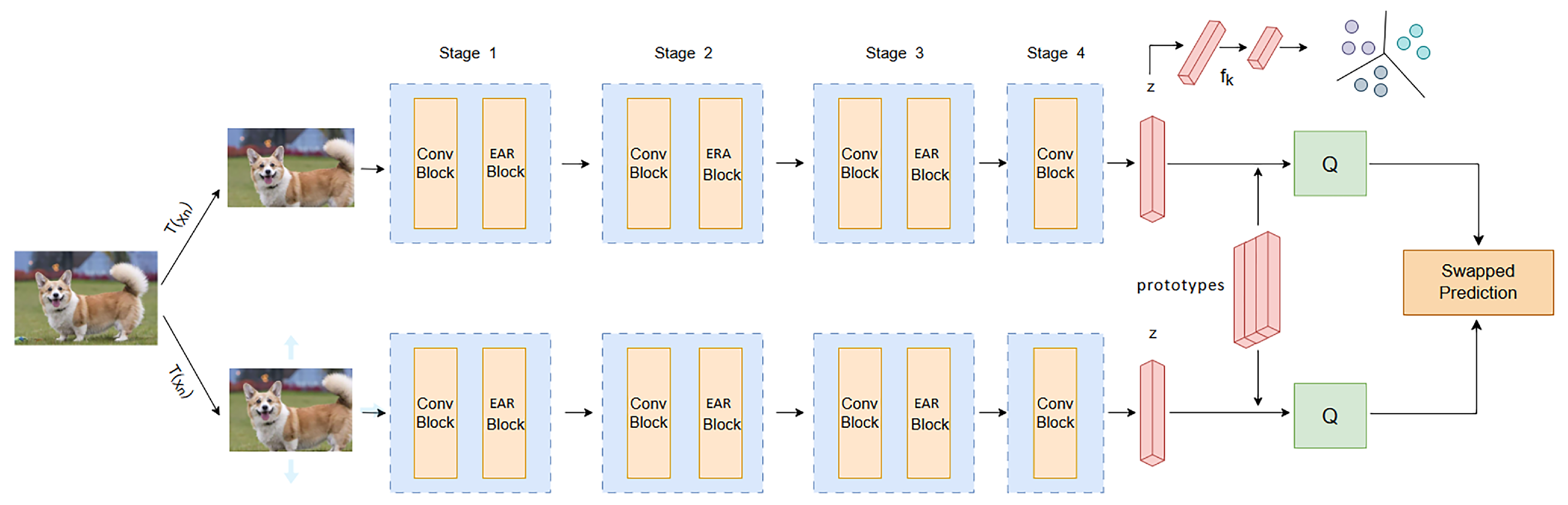
We elaborate the proposed end-to-end, multi-branch, feature fusion-comparison deep clustering method, which contains the multi-branch feature-aggregation module EAR, as shown in Figure 1. We model this end-to-end method as , specifying the image dataset to complete the nonlinear mapping of , where is the unlabeled input image, represents the clustering allocation result of its input image, and is the number of clusters in the cluster.
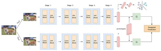
Figure 1.
Multi-branch, feature fusion-comparison deep clustering architecture. Firstly, a convolutional neural network that integrates multi-branch feature extraction strategies is used to extract high-dimensional representations. The Conv Block and the EAR Block iteratively interact with each other. The EAR uses a three-branch structure to identify spatial channel features and weighted receptive-field spatial features from different dimensions. Then, different transformed instances of the same data sample are mapped to the clustering center in the feature space, and the comparison of instance samples is completed through the clustering center. Finally, clustering is performed based on the embedded feature vector z.
3.1. Contrast Deep Clustering
For each image data sample in the fixed image dataset , we use different data transformation strategies , where represents transformations of the same data sample . The one-dimensional embedded compressed vector is obtained by embedding the data sample into the latent feature space using . is a feature-extraction network consisting of four stages, with the first three stages containing two basic building blocks, Conv Block and EAR Block, and the last stage containing only Conv Block. Conv Block uses convolutional kernel sliding to capture short neighborhood features, EAR Block captures multi-branch information with grouped subspace distribution, and Conv Block and EAR Block capture features through continuous iterative interaction.
In order to better remove interfering noise and obtain high-dimensional unsupervised semantic information, we adopt an unsupervised contrastive learning strategy. SimCLR [19], MOCO [12], and others require the construction of a large number of negative samples, which requires a significant amount of computing power and memory-resource consumption. We use the contrast learning strategy of SwAV [17] to solve the problem of the resource waste of negative samples by comparing cluster centers. Specifically, sample is transformed into different views, and ; based on the data-transformation strategy , forward propagation in the network yields vectors and . Due to the information-invariance mechanism of the image itself, different view instances of the same sample can be divided into the same cluster center. Therefore, instances under different views can exchange their predicted probability distribution, , to capture the same high-dimensional representation, which can be specifically defined as follows:
where code is the self-label probability distribution of two transformed views of the same sample, is the degree of fit between the feature and the probability distribution code , which can be calculated using cross-entropy loss, and p represents the computed assignment probability. The probability distribution obtained from an instance variant view is used for prediction using another view, where predicts , and predicts , thereby achieving exchange prediction and completing the comparison of positive samples between clusters based on cluster centers. The probability distribution of two exchanged views of the same sample and the calculated probability distribution are obtained through trainable cluster centers. The vector is mapped from different views to a set of trainable prototype vectors , which serve as trainable cluster centers and are continuously updated during iterative training. Simultaneously, is used to represent the column matrix composed of trainable prototype vectors. Next, the feature representation is compared with each prototype vector, utilizing the dot product of z and trainable prototype vectors to obtain the corresponding probability distribution:
where is the temperature parameter, and is the vector obtained based on different data change strategy views. is the trainable cluster center embedding of the Kth cluster. We use to calculate code so that all instances are equally partitioned by the prototype. This equal distribution constraint ensures that the distribution probabilities of different instances are different, thereby avoiding trivial solutions that may occur during the process of minimizing cross-entropy. Given feature vectors for training mini-batches, prototype vectors , with a probability distribution of , optimize the allocation probability to obtain the optimal one, thereby maximizing the correlation between the generated feature vectors and trainable prototypes:
where , is the mapping smoothness constraint term, and Q is the target assignment probability obtained from optimal transportation. The Sinkhorn–Knopp algorithm is used to solve coed q iteratively. A more detailed description of the SwAV and Sinkhorn–Knopp algorithms can be found in references [17,28,29].
Clustering clusters dynamically allocate along with the training of contrastive representation learning. The goal is to partition the feature vectors mapped by the network in the embedding space into different categories in an unsupervised manner. At this stage, predictive analysis is completed through the fully connected predictor , achieving . Firstly, the fully connected predictor achieves a fully connected mapping from the input feature to the output category . It predefines each sample to a different category, resulting in a one-dimensional probability output, . Since both and , calculated in Equation (2), are probability distributions based on the feature extracted via the encoder, mutual information [30] is used to maximize the dependency between the two probability distributions. Finally, convergence is achieved by mapping sample instances with similar semantics in to the same cluster in . The dependency measurement method based on mutual information can be defined as follows:
Specifically, inspired by the maximization of mutual information clustering strategy in IMC-SwAV [31], we utilize mutual information measurement methods to maximize the dependency between the assignment probability distribution and . By mapping semantically similar instances in to the same cluster in , the dependency between the two probability distributions is maximized to achieve convergence. It can be defined as follows:
where is the unsupervised classification prediction, , is the code obtained from Equation (2), , is a conditional entropy calculation, is used for marginal entropy calculation, is the introduction of a weighting parameter to constrain the marginal entropy, denotes the number of instances in batch size, denotes the total number of instances in batch size corresponding to the data-enhanced transformed views, and the indexes and denote the corresponding transformed views. To prevent overfitting of the fully connected predictor , we regularize using the marginal entropy from Equation (6), ensuring fair distribution of different sample instances within each cluster. Simultaneously, by minimizing the conditional entropy in Equation (6), we enhance the confidence of clustering predictions.
3.2. Multi-Branch Feature Aggregation
We propose a new basic building block EAR in the feature extraction network , which integrates multi-branch feature-aggregation methods. In this work, multiple sub-features are divided in the channel dimension, followed by establishing interaction between weighted receptive-field spatial features and spatial features in the feature extraction network, constructing long short-term dependencies to acquire information from different dimensional distributions, as shown in Figure 2. Specifically, first, the channel (C) dimension is divided into multiple spatial grouping sub-features (C//G), and the different semantic feature distributions within each subspace are meaningfully learned. Meanwhile, we adopt a three-branch parallel structure, which is defined as X-branch, Y-branch, and 3 × 3-branch, respectively. The X-branch and Y-branch perform feature mapping along the horizontal and vertical coordinate directions, respectively, while preserving spatial position information [32] and weighting receptive field information. The 3 × 3-branch establishes global dependencies and constructs relationships in different dimensions.
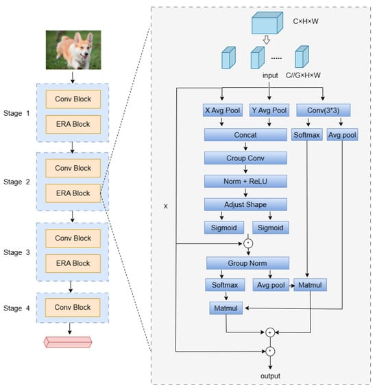
Figure 2.
A note on multi-branch feature aggregation modulo rapidity.
Each spatial group in the X-branch is C//G, given an input of dimension C//G × H × W. One-dimensional compressive encoding is completed along the W dimension, averaging pooling horizontal coordinate direction characteristics, which can be defined as follows:
For input features in the Y-branch, the average pooling is completed in the H-dimension, which can be formulated as follows (Figure 2):
The X-branch and Y-branch capture global feature information and positional information in the corresponding directions through compression encoding and then aggregate the features along the two branch directions. While retaining the horizontal and vertical coordinate position information, we will focus on receptive field features and measure the importance of different receptive field spatial features. Given the feature map , since convolutional kernel scanning can dynamically generate receptive field features, Group Conv is used to quickly extract receptive field spatial features. To define the importance of features at different positions during the sliding process of the wild window, a weighted mapping is given as a new feature, which can be formulated as follows:
where denotes the convolution kernel is a grouped convolution of i × i, and AvgPool extracts the global features of the given feature map . is used for information interaction computation, and Softmax is used to obtain the weighted values of receptive field features. Norm is used to normalize the features obtained from grouped convolution , followed by a ReLU activation for non-linear transformation. Subsequently, an Adjust Shape operation is performed to reshape the features. To consider the importance of each channel feature, multiplication is used for feature fusion to achieve inter-channel interaction among features.
The multi-branch feature-aggregation module EAR not only focuses on the receptive field feature distribution between spatial channels but also considers global encoding. In the 3 × 3-branch, the 3 × 3 convolution kernel is used to construct sub-features, extract multi-scale spatial features to expand the feature space, and capture some spatial structural information lost in the compression of the X-branch and Y-branch. Subsequently, the Avg pool is used to obtain global information encoding, which interacts with the X- and Y-branches to construct long short dependencies. EAR has established three branches for cross-dimensional interaction, learning spatial channel information and weighted receptive field spatial features from different dimensions and achieving the aggregation of multi-branch sub-features to improve clustering performance.
3.3. Objective Function
The end-to-end architecture we use is a single-stage integrated architecture that jointly optimizes comparative representation learning and clustering during training with the following overall objective distribution:
is the loss function for the comparison representation stage, and is the loss function for the clustering stage. The target loss of the overall architecture is summed up by the losses of the two stages, completing iterative optimization.
4. Experiments
We experimented with our proposed method on three commonly used image clustering datasets, and we evaluated the clustering performance by comparing evaluation metrics, demonstrating the effectiveness of the experiment.
4.1. Dataset
We present three challenging image datasets used in our approach, CIFAR-10 [33], CIFAR-100/20 [33], and STL10 [34], for which the basic details of the data are presented in Table 1, as well as a brief description of the different datasets.

Table 1.
Summary of datasets used for evaluation.
- CIFAR-10 [33] is a dataset containing 60,000 images of color objects, of which 50,000 are training images, and 10,000 are test images. Each image is a three-channel color RGB image of size 32 × 32. Each image in CIFAR-10 represents real-world objects and can be categorized into 10 classes: airplane, automobile, bird, cat, deer, dog, frog, horse, ship, and truck.
- CIFAR-100/20 [33] contains 60,000 color images, including 50,000 training images and 10,000 test images, each of which belongs to the RGB three-channel type of 32 × 32 pixels. The CIFAR100 dataset contains 100 categories, which can be subdivided into 20 major categories from a deeper perspective, and 5 subcategories in each major category. From the perspective of category division, CIFAR-100/20 is more detailed and rich in hierarchical structure than CIFAR-10, which is more conducive to network learning.
- STL10 [34] is one of the commonly used benchmark datasets in the unsupervised domain, which consists of 113,000 RGB images, all of which have a resolution of 96 × 96, and it contains 105,000 training data and 8000 test data.
4.2. Evaluation Metrics
In our experiments, we used three commonly applied unsupervised evaluation metrics to assess the clustering performance of our proposed method, namely the accuracy of comparative clustering (ACC), normalized mutual information (NMI), and the adjusted Rand index (ARI). The accuracy of comparative clustering (ACC) measures the mapping relationship between the predicted distribution and the true distribution, and it can be formulated as follows:
The ACC mapping range is within [0, 1], and the closer its value is to 1, the better the clustering effect. The standard mutual information (NMI) measures the similarity of the sample clustering results:
H(l) and H(c) correspond to the entropy values of the sample true labels and the sample predicted labels, respectively, and NMI takes values within [0, 1]; the larger its value, the better the clustering effect. The adjusted Rand index (ARI) measures the similarity between the sample clustering categories and the true categories:
In its formula, N is the total number of samples, a represents the number of true positives or TPs, b represents the number of true negatives or TNs, and ARI takes the value of [−1, 1]; a higher value indicates that the category obtained from clustering is more similar to the real category.
4.3. Experimental Settings
In the experiment, for the sake of fair comparison, we followed the settings in the benchmark methods SwAV [17] and IMC SwAV [31]. During training for all experiments, we used the PyTorch 2.0.1 architecture to implement our method, with the learning rate set to , using the Adam optimizer. Due to differences in data volume across different datasets, the batch size was set to 256. The number of channel feature groupings, G, in EAR was set to 8. For the fairness of the experiment, all data in the experimental section were trained using one NVIDIA RTX 4090 (https://www.autodl.com/) and 500 epochs of training data were obtained. The clustering results obtained from training on three datasets were reported.
4.4. Comparative Experiment
Based on three classic datasets, we compare our proposed method with classical clustering and comparative deep clustering algorithms. For a more fair comparison, all methods were run on a server with only one NVIDIA RTX 4090 GPU, and their experimental results were replicated in the same experimental environment and compared with our running results. As shown in Table 2, compared to the classical clustering algorithm k-means, deep clustering can substantially improve clustering performance compared to the simple clustering algorithm. Next, we will compare the deep clustering methods with the end-to-end mechanism and the multi-stage mechanism, respectively. The multi-stage mechanism SCAN exhibits separated multi-stage coupling during the training phase. Compared with multi-stage methods, SwEAC still has competitiveness, achieving an improvement of approximately 7% in all three indicators on the STL10 dataset. This proves that combining clustering objectives with network-optimization processes can significantly improve learning efficiency without overly relying on network initialization. Compared to other single-stage end-to-end mechanisms for deep clustering CC [26], our method achieves an ACC of 90.1 on the CIFAR-10 dataset within a unified architecture. Compared to CC [26], we obtained better clustering performance with limited computational resources (on a server with only 1 GPU on board). We and IMC-SwAV [31] both used the SwAV comparison mechanism [17] during the unsupervised representation learning phase. Our method achieved better clustering performance on all four datasets, especially CIFAR-100/20, with which improvements of 2% to 3% were achieved in the ACC, NMI, and ARI metrics, demonstrating the effectiveness of optimized representation learning.
Table 2.
Clustering performance using three object image benchmarks; note that all data were trained on an NVIDIA RTX 4090 to get the run results.
4.5. Empirical Analysis
4.5.1. Visualization of Cluster Semantics
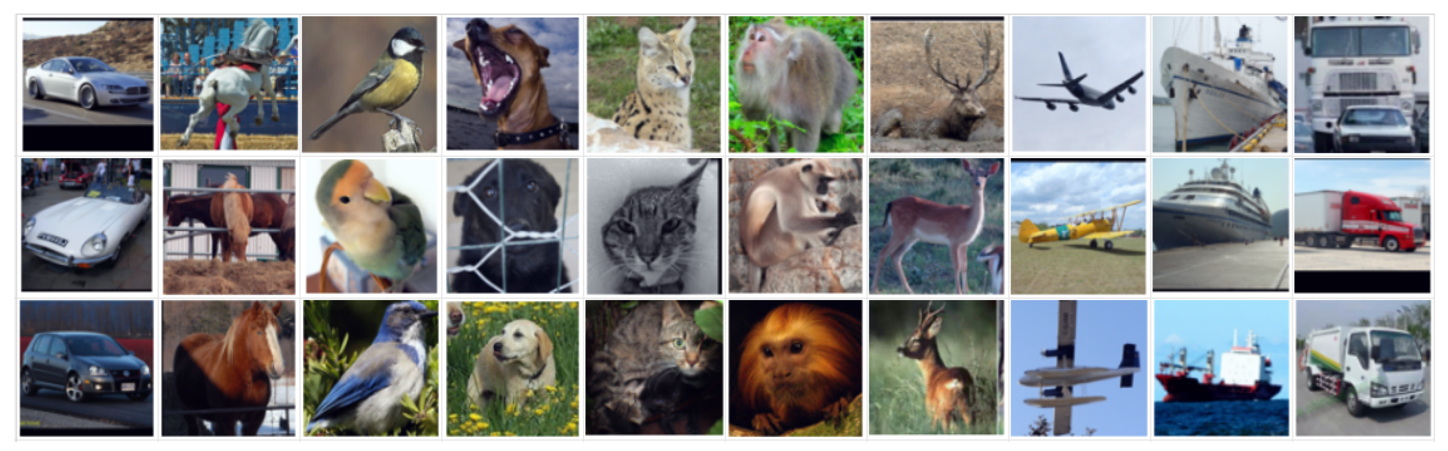
In our experiments, we visualized the semantic clustering done using SwEAC on the STL10 dataset based on the prototype samples, as shown in Figure 3. Specifically, we selected three samples from 10 clusters that were close to the cluster center and visualized their original images. The visualization results show that we learned semantically meaningful features, demonstrating that our network can extract higher-level semantic features for clustering assignment.
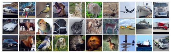
Figure 3.
Visualization of semantic clustering on STL10.
4.5.2. Ablation Study
To further demonstrate the effectiveness of the encoder (Encode) that integrates multi-branch aggregation features, we conducted ablation studies, exploring the impact of our proposed multi-branch feature aggregation module, EAR, on clustering performance. SwEAC (EAR) uses an encoder that aggregates multi-scale features. To demonstrate that the multi-branch feature extraction strategy in the deep learning stage can learn feature representations that are more conducive to clustering, we removed the multi-branch feature-aggregation module EAR and adopted the deep clustering model SwEAC (ResNet) of the ordinary encoder of the ordinary residual neural network [36]. As shown in Table 3, we conducted ablation experiments based on three datasets. The data in the table indicates that, in the deep clustering model with multi-branch feature fusion module SwEAC (EAR), ACC, NMI, and ARI have all shown varying degrees of improvement, increasing by 2.5%, 2.4%, and 2.6% respectively. On the STL10 dataset, all three clustering metrics showed slight improvements, with NMI further increasing by 0.4%. This confirms that it is effective and that fusing multi-scale feature aggregation methods can optimize representation learning and thus improve clustering performance, which can lead to learning better clustering-oriented feature representations.
Table 3.
Validity of the ablation study on three benchmark datasets.
4.6. Comparative Study
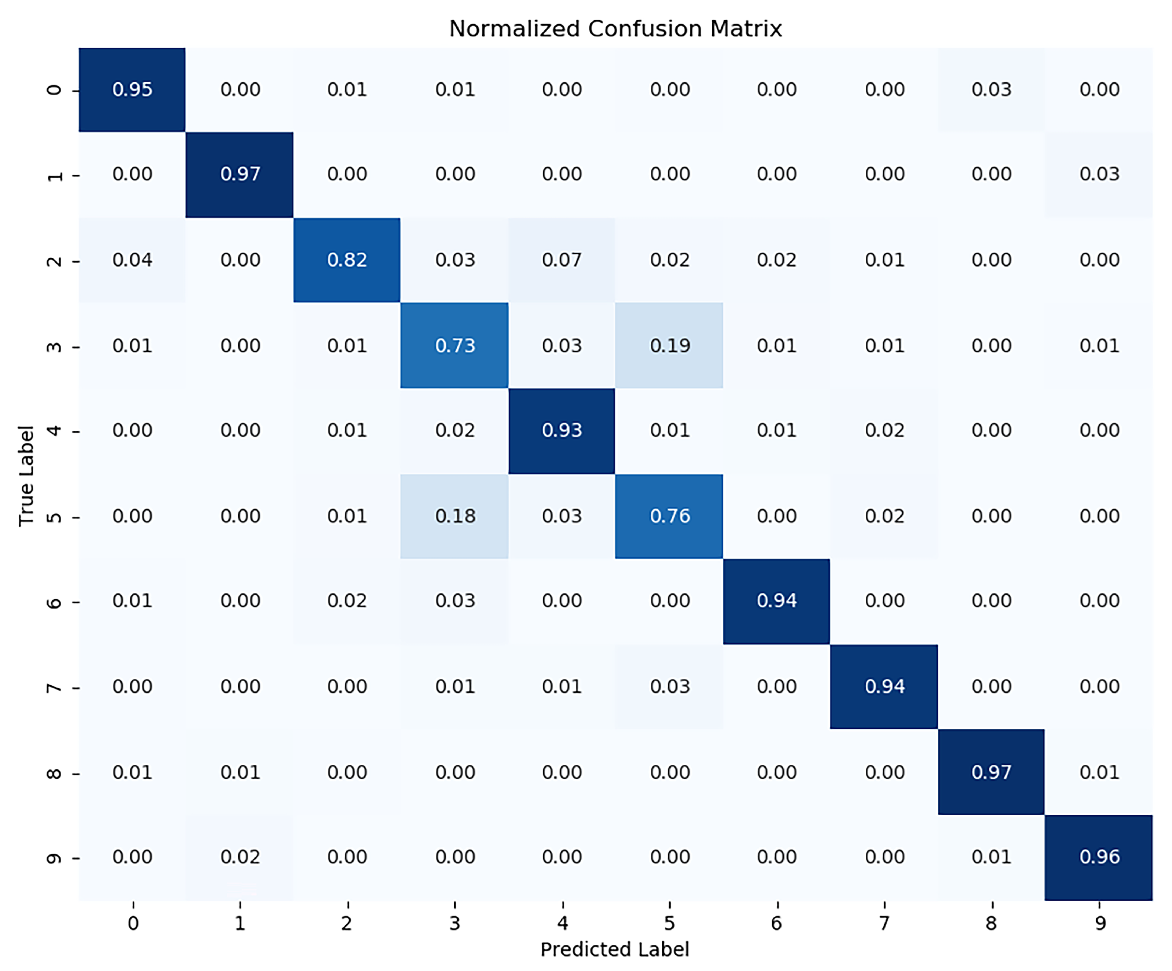
In order to demonstrate the effectiveness of the proposed comparative deep clustering algorithm, we replaced the clustering module and combined our model’s deep learning module with classical clustering algorithms for comparison. Specifically, K-means and spectral clustering (SC) are classic clustering algorithms, so we replaced the clustering module of SwEAC with k-means and spectral clustering (SC) algorithms, respectively. As shown in Table 4, the data in the table are derived from the experimental results on the CIFAR-10 dataset. We can see that our proposed SwEAC outperforms the K-means and spectral clustering (SC) models in all three clustering metrics. To further demonstrate the effectiveness of the SwEAC clustering model, we compared the clustering prediction results of each cluster with the true labels of the samples, generated corresponding confusion matrices, and completed normalization. As shown in Figure 4, we used a confusion matrix on the CIFAR-10 validation set to provide the correspondence between the predicted results and the actual true labels. The diagonal of the confusion matrix represents the degree to which the predicted results of the sample match the actual true labels.
Table 4.
Performance comparison based on multi-clustering methods.
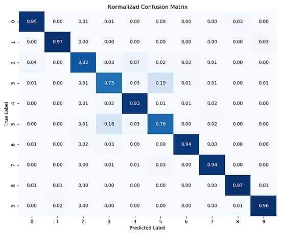
Figure 4.
Correspondence between predicted results and actual true labels in the confusion matrix.
4.7. Parameter Sensitivity
We conducted parameter sensitivity research in the multi-branch feature aggregation module and analyzed the impact of the multi-channel feature grouping parameter G in the multi-branch feature extraction module on clustering performance. As we divided the channel (C) dimension into multiple spatial grouping sub-features (C//G), we set G as a number divisible by C, which was 4, 8, 16, and 32. Based on the CIFAR-100/20 dataset, the clustering performance was compared under different parameter values. Table 5 shows the results at different G values.
Table 5.
SwEAC performance under different parameter settings on the CIFAR-100/20 dataset.
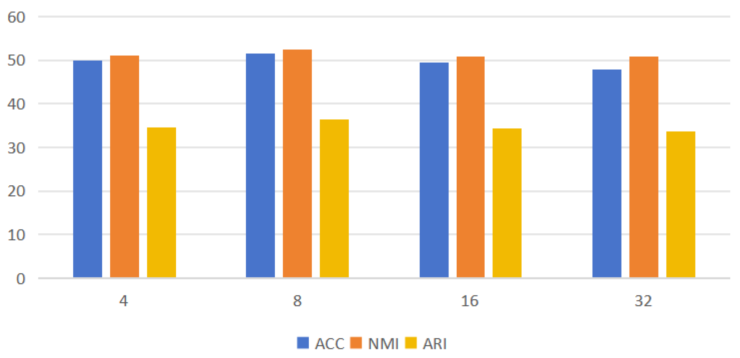
Figure 5 demonstrates the effect of different values of G taken on the clustering performance and evaluated with three metrics, ACC, NMI, and ARI. Here, we aim to evaluate the clustering performance under multi-space grouping subspace. The results in the figure show that the clustering performance metrics are all improved when the value of G is increased from 4 to 8, the performance is relatively better when G = 8, and the clustering performance is instead all decreased as G keeps increasing. It can be seen that, through proper multi-channel feature grouping, different semantic feature distributions within a meaningful multi-grouping subspace can be learned, leading to better clustering results.

Figure 5.
Performance of different G-element fetches; the horizontal coordinate indicates the G fetches.
5. Conclusions
The performance of clustering is largely influenced by representation learning; therefore, we propose an end-to-end, multi-branch, feature fusion-comparison deep clustering method. We integrate feature extraction and clustering tasks into a unified end-to-end architecture, using an encoder based on multi-branch information aggregation and applying a clustering-center comparison strategy to obtain better semantic features for clustering allocation. This method has shown good clustering performance on three popular datasets, and compared to popular comparative deep clustering methods, it has achieved certain improvements in all three clustering evaluation indicators. In future work, we have plans to apply it to datasets and learning tasks in other fields, such as semi-supervised learning. By using a small amount of labeled data to train the network, the learning capability of the feature extraction network is further enhanced, leading to improved clustering performance.
Author Contributions
Writing—original draft, X.L.; Writing—review & editing, H.Y. All authors have read and agreed to the published version of the manuscript.
Funding
This research was funded by Haikou Science and Technology Plan Project (2022-007, 2022-015).
Data Availability Statement
We used the publicly available datasets CIFAR-10, CIFAR-100/20, and STL10. The CIFAR-10 and CIFAR-100/20 datasets can be accessed at http://www.cs.toronto.edu/~kriz/cifar.html on 2 September 2024, and the STL10 datasets can be accessed on 2 September 2024 at https://cs.stanford.edu/~acoates/stl10/.
Conflicts of Interest
The authors declare no conflicts of interest.
References
- Li, F.; Qiao, H.; Zhang, B.; Xi, X. Discriminatively Boosted Image Clustering with Fully Convolutional Auto-Encoders. Pattern Recognit. 2018, 83, 161–173. [Google Scholar] [CrossRef]
- von Luxburg, U. A tutorial on spectral clustering. Stat. Comput. 2007, 17, 395–416. [Google Scholar] [CrossRef]
- Caron, M.; Bojanowski, P.; Joulin, A.; Douze, M. Deep Clustering for Unsupervised Learning of Visual Features; Springer: Berlin/Heidelberg, Germany, 2018; Volume 11218, pp. 139–156. [Google Scholar]
- Ting, C.; Simon, K.; Mohammad, N.; Geoffrey, H. A Simple Framework for Contrastive Learning of Visual Representations. In International Conference on Machine Learning; PMLR: Birmingham, UK, 2020; Volume 119, pp. 1597–1607. [Google Scholar]
- Xu, J.; Tang, H.; Ren, Y.; Peng, L.; Zhu, X.; He, L. Multi-level Feature Learning for Contrastive Multi-view Clustering. In Proceedings of the IEEE/CVF Conference on Computer Vision and Pattern Recognition 2022, New Orleans, LA, USA, 18–24 June 2022; Volume 1, pp. 16030–16039. [Google Scholar]
- Goodfellow, I.; Pouget-Abadie, J.; Mirza, M.; Xu, B.; Warde-Farley, D.; Ozair, S.; Courville, A.; Bengio, Y. Generative Adversarial Networks. arXiv 2014, arXiv:1406.2661. [Google Scholar] [CrossRef]
- Mirza, M.; Osindero, S. Conditional Generative Adversarial Nets. arXiv 2014, arXiv:1411.1784. [Google Scholar]
- Gansbeke, W.V.; Vandenhende, S.; Georgoulis, S.; Proesmans, M.; Gool, L.V. SCAN: Learning to Classify Images without Labels. In European Conference on Computer Vision 2020; Springer International Publishing: Cham, Switzerland, 2020; pp. 268–285. [Google Scholar]
- Chen, C.; Lu, H.; Wei, H.; Geng, X. Deep Subspace Image Clustering Network with Self-Expression and Self-Supervision; Springer: Berlin/Heidelberg, Germany, 2022; Volume 53, pp. 4859–4873. [Google Scholar]
- Yang, X.; Deng, C.; Zheng, F.; Yan, J.; Liu, W. Deep Spectral Clustering Using Dual Autoencoder Network. arXiv 2019, arXiv:1904.13113. [Google Scholar]
- Niu, C.; Shan, H.; Wang, G. SPICE: Semantic Pseudo-Labeling for Image Clustering. IEEE Trans. Image Process. 2022, 31, 7264–7278. [Google Scholar] [CrossRef]
- Kaiming, H.; Haoqi, F.; Yuxin, W.; Saining, X.; Ross, G. Momentum Contrast for Unsupervised Visual Representation Learning. In Proceedings of the IEEE/CVF Conference on Computer Vision and Pattern Recognition 2020, Seattle, WA, USA, 13–19 June 2020; Volume 2020, pp. 9726–9735. [Google Scholar]
- Xinlei, C.; Haoqi, F.; Ross, G.; Kaiming, H. Improved Baselines with Momentum Contrastive Learning. arXiv 2020, arXiv:2003.04297. [Google Scholar]
- Xie, J.; Girshick, R.; Farhadi, A. Unsupervised Deep Embedding for Clustering Analysis. arXiv 2016, arXiv:1511.06335. [Google Scholar]
- Wu, Z.; Xiong, Y.; Yu, S.X.; Lin, D. Unsupervised Feature Learning via Non-Parametric Instance Discrimination. In Proceedings of the IEEE Conference on Computer Vision and Pattern Recognition 2018, Salt Lake City, UT, USA, 8–22 June 2018. [Google Scholar]
- van den Oord, A.; Li, Y.; Vinyals, O. Representation Learning with Contrastive Predictive Coding. arXiv 2018, arXiv:1807.03748. [Google Scholar]
- Caron, M.; Misra, I.; Mairal, J.; Goyal, P.; Bojanowski, P.; Joulin, A. Unsupervised Learning of Visual Features by Contrasting Cluster Assignments. Adv. Neural Inf. Process. Syst. 2020, 33, 9912–9924. [Google Scholar]
- Jean-Bastien, G.; Florian, S.; Florent, A.; Corentin, T.; H., R.P.; Elena, B.; Carl, D.; Avila, P.B.; Daniel, G.Z.; Gheshlaghi, A.M.; et al. Bootstrap Your Own Latent—A New Approach to Self-Supervised Learning. Adv. Neural Inf. Process. Syst. 2020, 33, 21271–21284. [Google Scholar]
- Chen, X.; He, K. Exploring Simple Siamese Representation Learning. In Proceedings of the IEEE/CVF Conference on Computer Vision and Pattern Recognition 2021, Nashville, TN, USA, 20–25 June 2021; pp. 15745–15753. [Google Scholar]
- Chen, X.; Xie, S.; He, K. An Empirical Study of Training Self-Supervised Vision Transformers. arXiv 2021, arXiv:2104.02057. [Google Scholar]
- Caron, M.; Touvron, H.; Misra, I.; Jégou, H.; Mairal, J.; Bojanowski, P.; Joulin, A. Emerging Properties in Self-Supervised Vision Transformers. arXiv 2021, arXiv:2104.14294. [Google Scholar]
- Vaswani, A.; Shazeer, N.; Parmar, N.; Uszkoreit, J.; Jones, L.; Gomez, A.N.; Kaiser, L.; Polosukhin, I. Attention Is All You Need. Adv. Neural Inf. Process. Syst. 2017, 30, 5998–6008. [Google Scholar]
- Guo, X.; Gao, L.; Liu, X.; Yin, J. Improved Deep Embedded Clustering with Local Structure Preservation. In Proceedings of the IJCAI 2017, Melbourne, Australia, 19–25 August 2017; pp. 1753–1759. [Google Scholar]
- Mukherjee, S.; Asnani, H.; Lin, E.; Kannan, S. Clustergan: Latent Space Clustering in Generative Adversarial Networks. arXiv 2019, arXiv:1809.03627. [Google Scholar] [CrossRef]
- Hu, J.; Zhang, Y.; Zhao, D.; Yang, G.; Chen, F.; Zhou, C.; Chen, W. A Robust Deep Learning Approach for the Quantitative Characterization and Clustering of Peach Tree Crowns Based on UAV Images. IEEE Trans. Geosci. Remote. Sens. 2022, 60, 1–13. [Google Scholar] [CrossRef]
- Li, Y.; Hu, P.; Liu, Z.; Peng, D.; Zhou, J.T.; Peng, X. Contrastive Clustering. In Proceedings of the AAAI Conference on Artificial Intelligence 2021, Virtually, 2–9 February 2021; Volume 35, pp. 8547–8555. [Google Scholar]
- Zhong, H.; Wu, J.; Chen, C.; Huang, J.; Deng, M.; Nie, L.; Lin, Z.; Hua, X.S. Graph Contrastive Clustering. arXiv 2021, arXiv:2104.01429. [Google Scholar]
- Cuturi, M. Sinkhorn Distances: Lightspeed Computation of Optimal Transportation Distances. arXiv 2013, arXiv:1306.0895. [Google Scholar]
- Peyré, G.; Cuturi, M. Computational Optimal Transport. arXiv 2019, arXiv:1803.00567. [Google Scholar]
- Hu, Q.; Zhang, L.; Zhang, D.; Pan, W.; An, S.; Pedrycz, W. Measuring relevance between discrete and continuous features based on neighborhood mutual information. Expert Syst. Appl. 2011, 38, 10737–10750. [Google Scholar] [CrossRef]
- Ntelemis, F.; Jin, Y.; Thomas, S.A. Information maximization clustering via multi-view self-labelling. Knowl.-Based Syst. 2022, 250, 109042. [Google Scholar] [CrossRef]
- Ouyang, D.; He, S.; Zhan, J.; Guo, H.; Huang, Z.; Luo, M.; Zhang, G. Efficient Multi-Scale Attention Module with Cross-Spatial Learning. arXiv 2023, arXiv:2305.13563. [Google Scholar]
- Krizhevsky, A.; Hinton, G. Learning Multiple Layers of Features from Tiny Images. 2009. Available online: https://www.cs.toronto.edu/~kriz/learning-features-2009-TR.pdf (accessed on 2 September 2024).
- Coates, A.; Ng, A.Y.; Lee, H. An Analysis of Single-Layer Networks in Unsupervised Feature Learning. In Proceedings of the Fourteenth International Conference on Artificial Intelligence and Statistics 2011, Fort Lauderdale, FL, USA, 11–13 April 2011; pp. 215–223. [Google Scholar]
- Znalezniak, M.; Rola, P.; Kaszuba, P.; Tabor, J.; Smieja, M. Contrastive Hierarchical Clustering. arXiv 2023, arXiv:2303.03389. [Google Scholar]
- Gao, H.; Liu, Z.; Weinberger, K.; van der Maaten, L. Deep residual learning for image recognition. In Proceedings of the IEEE Conference on Computer Vision and Pattern Recognition 2016, Las Vegas, NV, USA, 27–30 June 2016. [Google Scholar]

Disclaimer/Publisher’s Note: The statements, opinions and data contained in all publications are solely those of the individual author(s) and contributor(s) and not of MDPI and/or the editor(s). MDPI and/or the editor(s) disclaim responsibility for any injury to people or property resulting from any ideas, methods, instructions or products referred to in the content. |
© 2024 by the authors. Licensee MDPI, Basel, Switzerland. This article is an open access article distributed under the terms and conditions of the Creative Commons Attribution (CC BY) license (https://creativecommons.org/licenses/by/4.0/).