

The Concept of Topological Derivative for Eigenvalue Optimization Problem for Plane Structures

Abstract
1. Introduction
2. Topological Derivative
2.1. Plane Structures
2.1.1. Existence of the Topological Derivative
2.1.2. Topological Sensitivities
2.2. Eigenvalue Problem
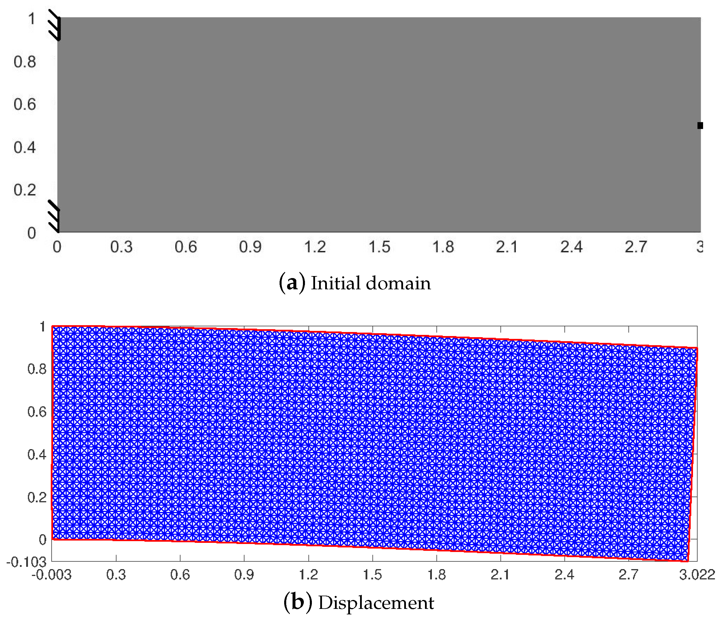
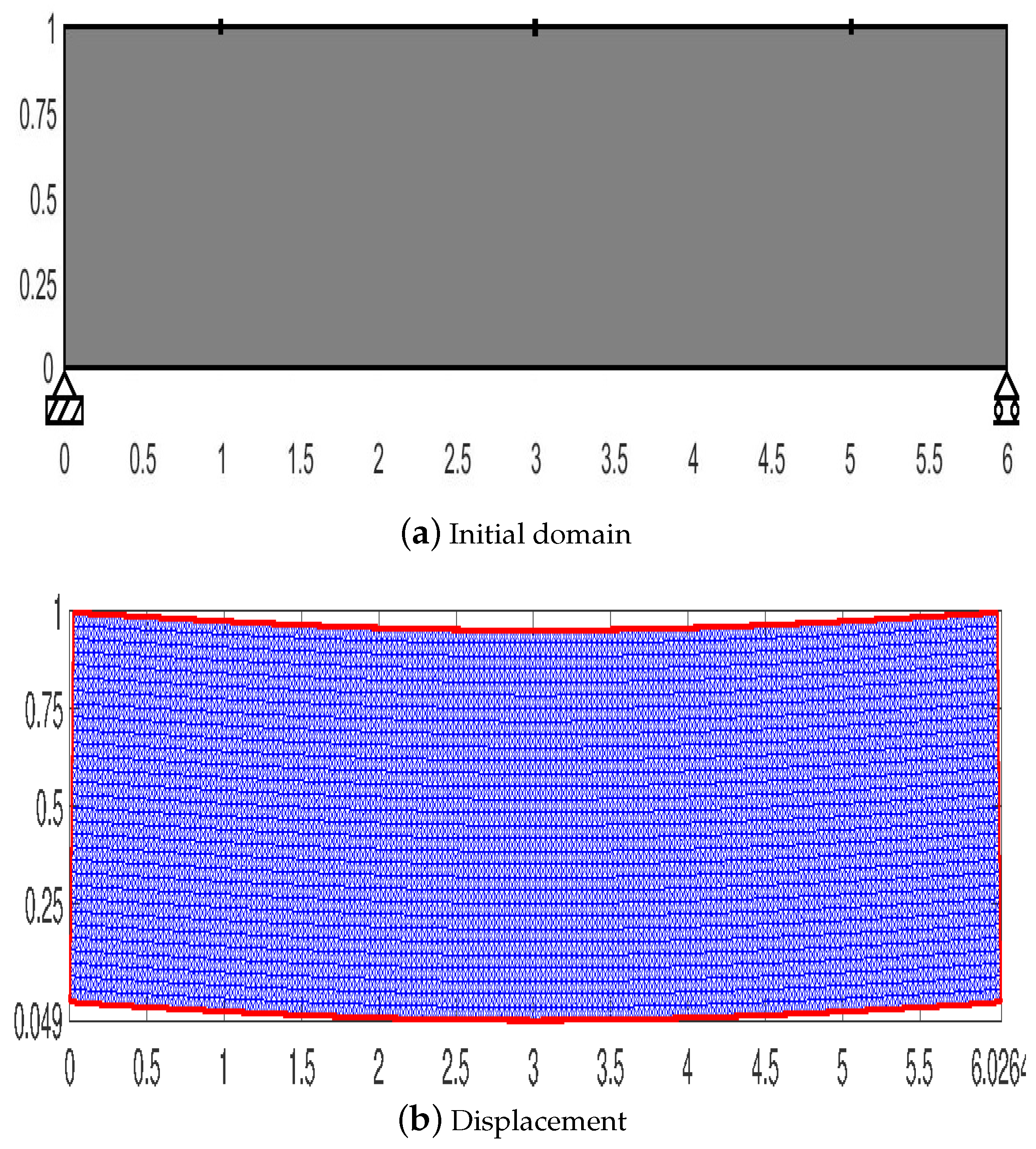
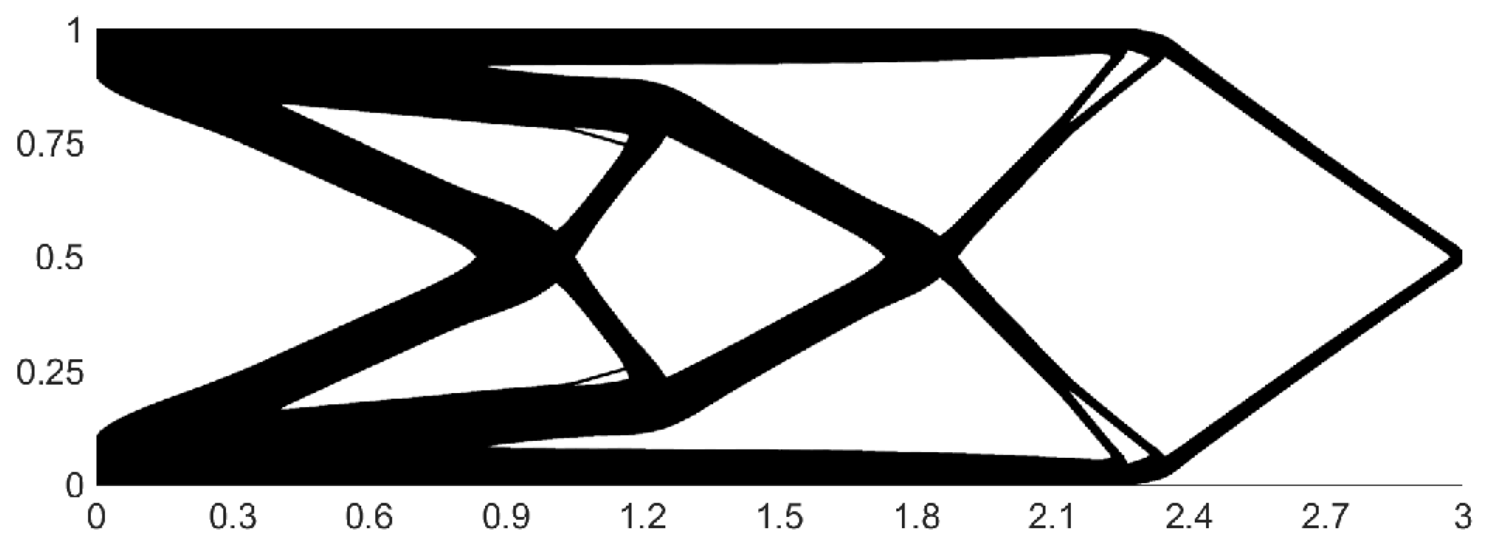
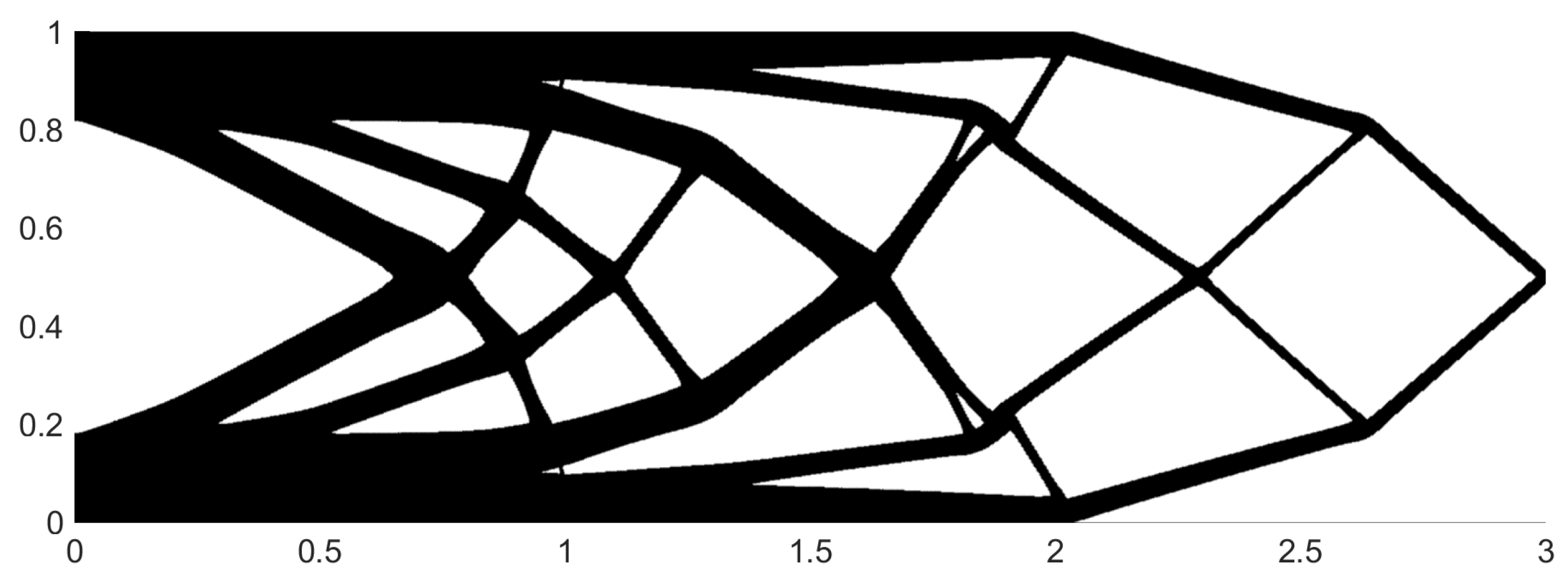
3. Numerical Results
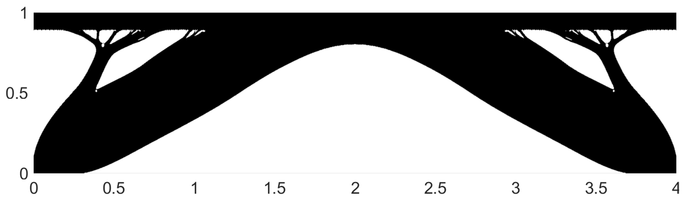
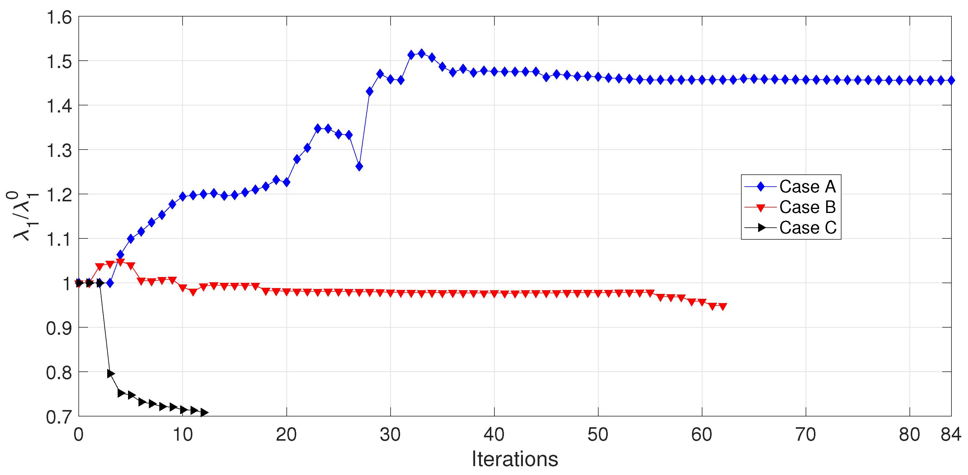
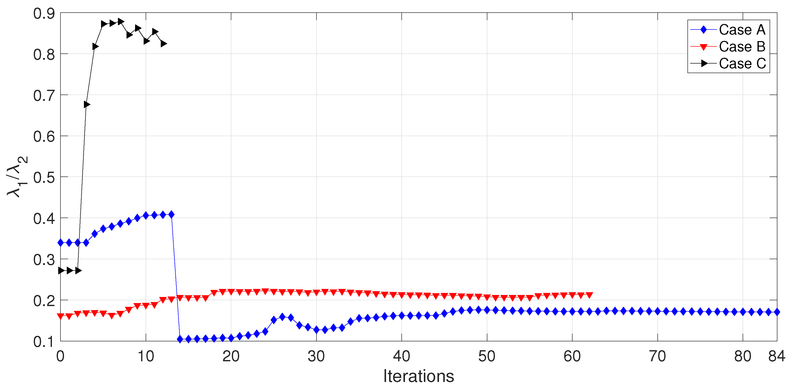
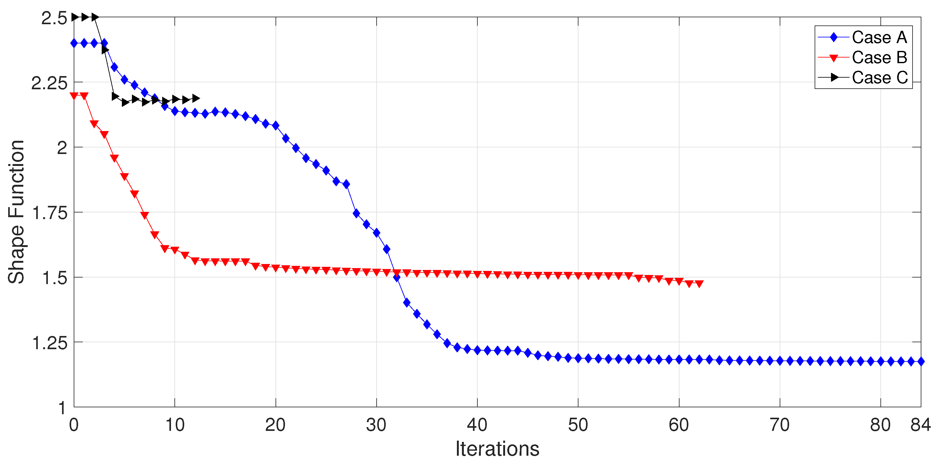
First Eigenvalue Maximization
4. Conclusions
Author Contributions
Funding
Data Availability Statement
Acknowledgments
Conflicts of Interest
Appendix A. Topological Asymptotic Analysis
Appendix A.1. Proof of Theorem 1
Appendix A.2. Proof of Theorem 2
References
- Masur, E.F.; Mroz, Z. Non-stationary optimality conditions in structural design. Int. J. Solids Struct. 1979, 15, 503–512. [Google Scholar] [CrossRef]
- Haug, E.J.; Rousselet, B. Design sensitivity analysis in structural mechanics. II. eigenvalue variationsi. J. Struct. Mech. 1979, 8, 161–186. [Google Scholar] [CrossRef]
- Seyranian, A.P.; Lund, E.; Olhoff, N. Multiple eigenvalues in structural optimization problems. Struct. Optim. 1994, 8, 207–227. [Google Scholar] [CrossRef]
- Jensen, J.S.; Pedersen, N.L. On maximal eigenfrequency separation in two-material structures: The 1D and 2D scalar cases. J. Sound Vib. 2006, 289, 967–986. [Google Scholar] [CrossRef]
- Gravesen, J.; Evgrafov, A.; Nguyen, D.M. On the sensitivities of multiple eigenvalues. Struct Multidiscip Optim 2011, 44, 583–587. [Google Scholar] [CrossRef]
- Torii, A.; Faria, J.R. Structural optimization considering smallest magnitude eigenvalues: A smooth approximation. J. Braz. Soc. Mech. Sci. Eng. 2017, 39, 1745–1754. [Google Scholar] [CrossRef]
- Ammari, H.; Khelifi, A. Electromagnetic scattering by small dielectric inhomogeneities. J. Math. Pures Appl. 2003, 82, 749–842. [Google Scholar] [CrossRef]
- Nazarov, S.A.; Sokołowski, J. Spectral problems in the shape optimisation. Singular boundary perturbations. Asymptot. Anal. 2008, 56, 159–204. [Google Scholar]
- Amstutz, S. Augmented Lagrangian for cone constrained topology optimization. Comput. Optim. Appl. 2011, 101–122. [Google Scholar] [CrossRef]
- Carvalho, F.; Ruscheinsky, D.; Giusti, S.; Anflor, C.; Novotny, A. Topological Derivative-Based Topology Optimization of Plate Structures Under Bending Effects. Struct. Multidiscip. Optim. 2020, 63, 617–630. [Google Scholar] [CrossRef]
- Ruscheinsky, D.; Carvalho, F.S.; Anflor, C.; Novotny, A.A. Topological asymptotic analysis of a diffusive–convective–reactive problem. Eng. Comput. 2020, 38, 477–500. [Google Scholar] [CrossRef]
- Takezawa, A.; Nishiwaki, S.; Kitamura, M. Shape and topology optimization based on the phase field method and sensitivity analysis. J. Comput. Phys. 2010, 229, 2697–2718. [Google Scholar] [CrossRef]
- Qian, M.; Hu, X.; Zhu, S. A phase field method based on multi-level correction for eigenvalue topology optimization. Comput. Methods Appl. Mech. Eng. 2022, 401, 115646. [Google Scholar] [CrossRef]
- Amstutz, S.; Andrä, H. A new algorithm for topology optimization using a level-set method. J. Comput. Phys. 2006, 216, 573–588. [Google Scholar] [CrossRef]
- Novotny, A.A.; Sokołowski, J. Topological Derivatives in Shape Optimization; Interaction of Mechanics and Mathematics; Springer: Berlin/Heidelberg, Germany, 2013; p. 324. [Google Scholar]
- Novotny, A.A.; Sokolowski, J. An Introdution to the Topological Derivative Method; Springer Briefs in Mathematics; Springer: New York, NY, USA, 2020. [Google Scholar]


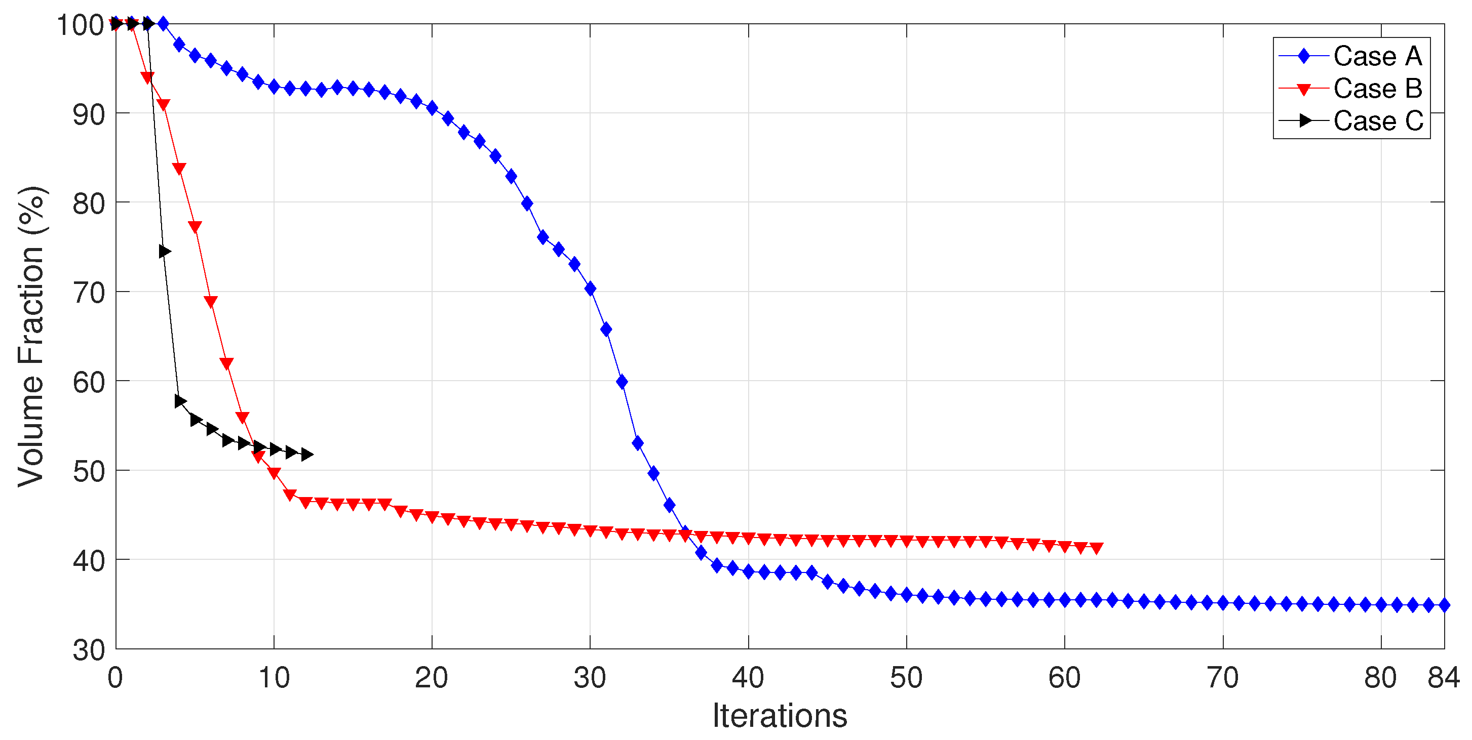
| Cases | Grid | Elements | Nodes | ||
|---|---|---|---|---|---|
| A | 10,800 | 5521 | 0.25 | 1.4 | |
| B | 21,600 | 11,011 | 0.3 | 0.7 | |
| C | 1600 | 851 | 0.3 | 1.5 |
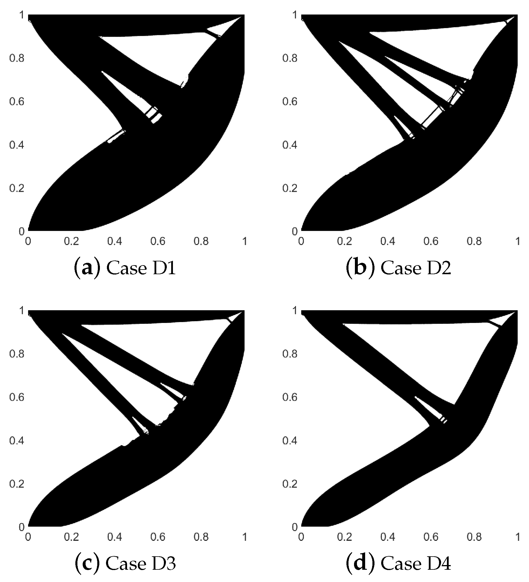
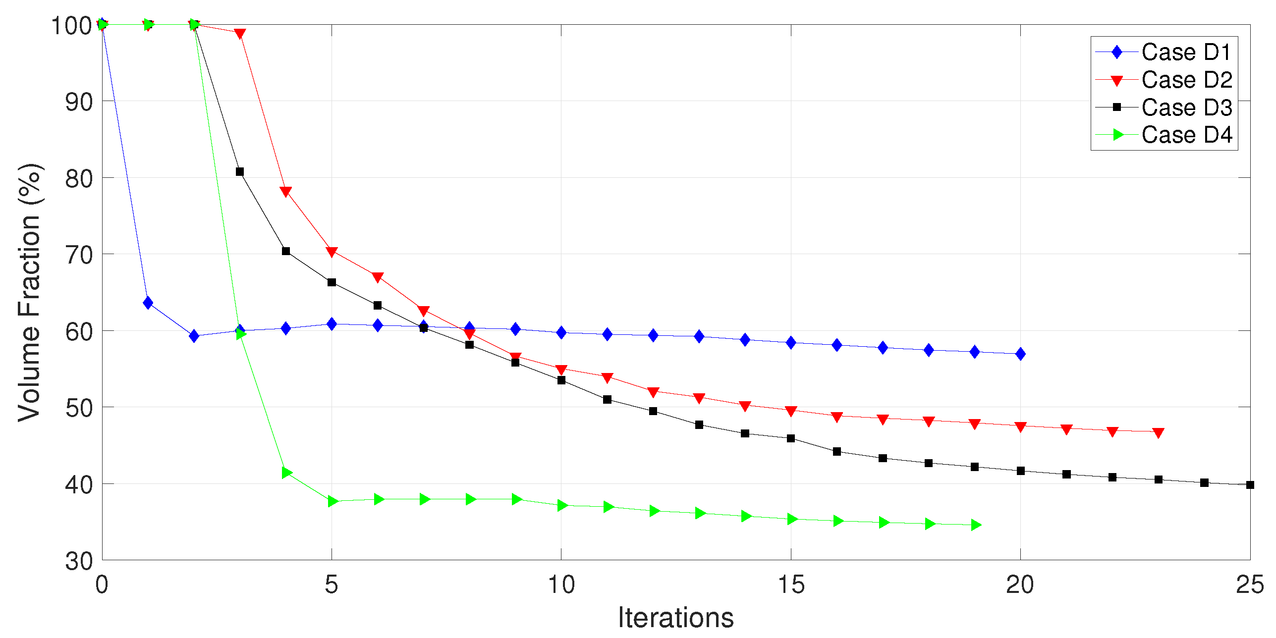
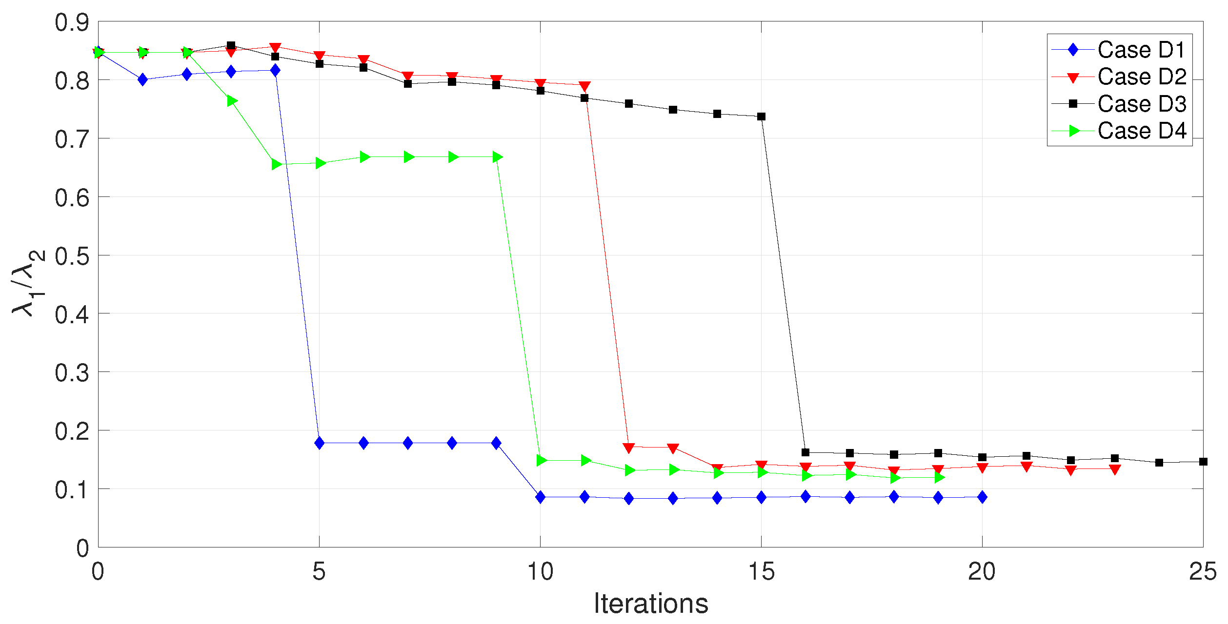
| Case D1 | Case D2 | Case D3 | Case D4 | |
|---|---|---|---|---|
Disclaimer/Publisher’s Note: The statements, opinions and data contained in all publications are solely those of the individual author(s) and contributor(s) and not of MDPI and/or the editor(s). MDPI and/or the editor(s) disclaim responsibility for any injury to people or property resulting from any ideas, methods, instructions or products referred to in the content. |
© 2024 by the authors. Licensee MDPI, Basel, Switzerland. This article is an open access article distributed under the terms and conditions of the Creative Commons Attribution (CC BY) license (https://creativecommons.org/licenses/by/4.0/).
Share and Cite
Carvalho, F.S.; Anflor, C.T.M. The Concept of Topological Derivative for Eigenvalue Optimization Problem for Plane Structures. Mathematics 2024, 12, 2762. https://doi.org/10.3390/math12172762
Carvalho FS, Anflor CTM. The Concept of Topological Derivative for Eigenvalue Optimization Problem for Plane Structures. Mathematics. 2024; 12(17):2762. https://doi.org/10.3390/math12172762
Chicago/Turabian StyleCarvalho, Fernando Soares, and Carla Tatiana Mota Anflor. 2024. "The Concept of Topological Derivative for Eigenvalue Optimization Problem for Plane Structures" Mathematics 12, no. 17: 2762. https://doi.org/10.3390/math12172762
APA StyleCarvalho, F. S., & Anflor, C. T. M. (2024). The Concept of Topological Derivative for Eigenvalue Optimization Problem for Plane Structures. Mathematics, 12(17), 2762. https://doi.org/10.3390/math12172762