Abstract
In the present work, we investigate certain algebraic and differential properties of the orthogonal polynomials with respect to a discrete–continuous Sobolev-type inner product defined in terms of the Jacobi measure.
Keywords:
orthogonal polynomials; Jacobi polynomials; recurrence relations; polar polynomials; location of zeros; asymptotic behavior MSC:
42C05; 33C45; 12D10; 34D05
1. Introduction
Let us consider a measure supported on the subset of the complex plane .
In the vector space of polynomials with complex coefficients , let us introduce the following inner product:
assuming that the integral exists. The inner product Equation (1) is called discrete–continuous Sobolev-type, which is a particular case of the Sobolev-type inner products. Algebraic and analytical properties and the limiting behavior of the families of orthogonal polynomials with respect to Sobolev-type inner products have been thoroughly used for the last 25 years. For an overview of this subject, see [1], or the introduction of [2] as well as [3].
Discrete–continuous Sobolev inner products were introduced in [4] to study the behavior of the optimal polynomial approximation of absolutely continuous functions in the norm generated by a Sobolev inner product as Equation (1). Later, in [5], R. Koekoek considered the Laguerre case with , , and . The Gegenbauer case was studied by Bavinck and Meijer in [6,7], with , , and and .
The families of orthogonal polynomials with respect to Equation (1) have been studied as an extension of the Bochner–Krall theory (i.e., polynomial sequences which are simultaneously eigenfunctions of a differential operator and orthogonal with respect to an inner product), see for the discrete–continuous case [8,9,10].
The starting point of our work is the orthogonality with respect to the Jacobi case. Let be the monic orthogonal polynomial sequence with respect to the Sobolev inner product
where , is a path encircling the points and first in a positive sense and then in a negative sense, as shown in Figure 2.1 in [11], and .
Let us consider as the monic Jacobi polynomials, i.e., the monic orthogonal polynomial sequence with respect to the measure . Therefore, for each n, satisfies
and let be the polynomial primitive of that has a zero at , i.e., for all , we have
Then, by definition of , it is clear that for all . It is straightforward to prove that the polynomial of degree n which is orthogonal with respect to Equation (2) can be written as follows (one must consider ):
where is called the polar polynomial associated with (see [12]) and from now on will be called the pole. Let us define the differential operator as
where is the Sobolev space of index 1. Taking into account that is orthogonal with respect to the inner product Equation (2), we have
for . Therefore, is the monic orthogonal polynomial of degree n with respect to the differential operator , and the measure (see [12,13,14,15,16,17]). In such a case, for , we have
The main aim of this work is to study algebraic (zero localization) and differential properties of the polynomial sequences that are orthogonal with respect to the inner product Equation (2) for the Jacobi weight case, which is a natural extension of the Legendre case [12].
2. Algebraic Properties of the Polar Jacobi Polynomials
Let us start by summarizing some basic properties of the Jacobi orthogonal polynomials to be used in the sequel to Chapter 18 in [18]
Proposition 1.
Let be the classical monic Jacobi orthogonal polynomial sequence. The following statements hold:
- 1.
- Three-term recurrence relation.with initial condition , and recurrence coefficients
- 2.
- First structure relation.with coefficients
- 3.
- Second structure relation.
- 4.
- Squared Norm. For every ,
- 5.
- Second-order difference equation. For every ,
- 6.
- Forward shift operator.
- 7.
- Asymptotic formula. Let . Put where the branch of the square root is chosen so that for . Then,where is a function of α and β and x independent of n. The relation holds uniformly on compact sets of .
Let us obtain the algebraic relations between the Jacobi polynomials and the polar Jacobi polynomials.
Lemma 1.
For any . The polar Jacobi polynomials can be written in terms of the Jacobi polynomials as follows:
Therefore,
Proof.
From Equation (6), we have
Therefore, by using the forward shift operator Equation (12), we have
From Equation (17), the identity (14) follows. Using Equation (14) and the second structure relation (9) the expression (16) follows.
Let us now to prove Equation (15): by using the second-order differential Equation (11) with being shifted to , respectively, and the forward shift operator of the Jacobi polynomials, we obtain
By using the differential Equation (18) and the identity
then Equation (15) follows and hence the result holds. □
The following additional property of orthogonality holds.
Theorem 1.
The polar Jacobi polynomial with pole fulfills the following property of orthogonality:
Furthermore, if , then
Proof.
Theorem 2.
The sequence of polar Jacobi polynomials with pole satisfies the following recurrence relation:
with initial conditions and , and coefficients
Proof.
Let the sequence be such that
where .
Then, by using Equation (6), we obtain
By the property of orthogonality Equation (19), we have
for .
On the other hand, let us denote
From the orthogonality of the Jacobi polynomials and the property of orthogonality (20), we obtain
Thus, multiplying Equation (22) by , integrating over , and using Equations (23) and (24), we obtain
The expression (21) is obtained after a straightforward calculation. □
A direct consequence of this result is the following.
Corollary 1
(The polar ultraspherical case). The sequence of symmetric polar Jacobi polynomials with pole , i.e., the sequence of polar ultraspherical polynomial with pole , satisfies, namely , the following recurrence relation:
with initial conditions and .
Another direct consequence is the fact that when one, or both, of the parameters is a negative integer, we can factorize the Jacobi polynomial. In fact (see (1.2) in [11]),
Remark 1.
Since in some results we will consider the polar Jacobi polynomials with different parameters and poles, to avoid such possible confusion, we will denote by the polar Jacobi polynomial of degree n with parameters α and β, and pole at ξ.
Corollary 2
(The factorization). For any positive integer k, the following identities hold:
Moreover, the recurrence coefficients satisfy the following relations:
and
Proof.
The identities (28)–(31) follow by using the factorization of the Jacobi polynomials Equations (26) and (27). In order to obtain the relation between the recurrence coefficients defined in Theorem 2, we must use the former factorization(s), and after a straightforward calculation the identities follow. □
The last result of this section is due the parity relation of the Jacobi polynomials, i.e.,
Lemma 2.
For any , the following identity holds:
3. Zero Location
Finding the roots of polynomials is a problem of interest in both mathematics and in areas of application such as physical systems, which can be reduced to solving certain equations. There are very interesting geometric relationships between the roots of a polynomial and those of . The most important result is the following.
Theorem 3
(The Gauß–Lucas theorem [19]). Let be a polynomial of degree of at least one. All zeros of lie in the convex hull of the zeros of the zeros of .
In this section, we are going to study the zero distribution for the polar Jacobi polynomials. The next result, which was obtained by G. Szegő, is useful to estimate where such zeros are located.
Theorem 4
(Szegő’s theorem [20,21]). Let and be polynomials of the form
If the zeros of lie in a closed disk and , …, are the zeros of , then the zeros of the “composition” of the two
have the form , where .
By using this result, we are going to locate the disk within which all the zeros of the polar Jacobi are located.
Theorem 5.
For any and , the zeros of lie inside the closed disk .
Proof.
Starting from Equation (6) and assuming that
where , then . In order to apply Szegő’s theorem, we consider
If , then , so . Moreover, if , i.e., is a zero of , then . Therefore, combining these inequalities and applying Szegő’s theorem one obtains that if , i.e., is a zero of , then and hence the result follows. □
In Figure 1, we illustrate on the one hand how accurate Theorem 5 is, and on the other hand, we show the behavior of the zeros of the same polar Jacobi polynomial when the pole travels along a specific circle (observe ).
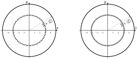
Figure 1.
Left: Zeros of the polar Jacobi polynomial for . Right: Zeros of the polar Jacobi polynomial for .
In Figure 2, we illustrate an example of Jacobi polar polynomials where the parameters or ; therefore, the zeros of the Jacobi polynomial can move away from the interval in a somewhat uncontrolled way. Therefore, Theorem 5 cannot be applied in such a case. However, observe that in the considered example .
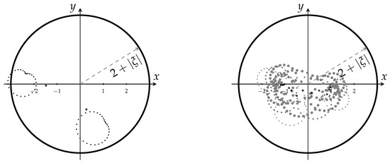
Figure 2.
Left: Zeros of the polar Jacobi polynomial for (dots) and zeros of the Jacobi polynomials (circles). Right: Zeros of the polar Jacobi polynomial for (gray dots) and zeros of the Jacobi polynomials (+,×, and circles) for , .
The next theorem gives the location of the zeros of the polar Jacobi polynomial of degree n and its multiplicity, or equivalently the location of source points and their corresponding strength.
Theorem 6.
For any and . The following statements hold:
- 1.
- If is a zero of , then is a zero of .
- 2.
- If is a zero of , then ζ is a zero of .
- 3.
- The zeros of have multiplicity of at most 2 and their multiple zeros are located on .
- 4.
- All the zeros of are located on the curve
Proof.
The first statement holds true due to Equation (34), the second statement holds true due to Equation (6), and the fourth statement holds true due to Equation (14).
Suppose that is a zero of multiplicity greater than two; then, by (6), is a zero of and also a zero of . Thus, is a zero of multiplicity 2 of . This is a contradiction since the zeros of the Jacobi polynomials are all simple. Therefore, statement 3 holds true. □
Remark 2.
- Observe that the zeros of do not have to be simple. Let or ; then, the polar polynomial of degree two , or .
- When the parameters are not standard, i.e., or then, by Corollary 2, statement 3 of Theorem 6 is no longer true. For example, if , , and , then .
We can establish the following result concerning the boundedness of the zeros of the polar polynomials.
Lemma 3.
Given , let us define the two numbers and . Then, the following can be stated:
- 1.
- All zeros of the polar Jacobi polynomials with pole ξ are contained in .
- 2.
- If , the zeros of the polar Jacobi polynomials with pole ξ are simple and contained in the exterior of the ellipse , where .
Proof.
By Equation (14), the zeros of are located in . Since , they are contained in the interior of the set . It is known that the zeros of , namely , satisfy . Therefore, for any , such that , we have
Hence, the first statement holds.
Concerning the second statement, let z be such that . From the well-known arithmetic–geometric mean inequality, we have
If is a zero of , we obtain, in view of Equation (34),
Therefore, the result holds. □
The last result is about the asymptotic behavior of the zeros of the polar Jacobi polynomials.
Theorem 7
(Theorem 22 in [16]). The accumulation points of zeros of are located on the set , where is the ellipse
where .
Funding
This research received no external funding.
Data Availability Statement
The original contributions presented in the study are included in the article, further inquiries can be directed to the corresponding author.
Conflicts of Interest
The author declares no conflicts of interest.
References
- Martínez-Finkelshtein, A. Analytic aspects of Sobolev orthogonal polynomials revisited. J. Comput. Appl. Math. 2001, 127, 255–266. [Google Scholar] [CrossRef]
- Lagomasino, G.L.; Español, F.M.; Cabrera, H. Logarithmic asymptotics of contracted Sobolev extremal polynomials on the real line. J. Approx. Theory 2006, 143, 62–73. [Google Scholar] [CrossRef][Green Version]
- Marcellán, F.; Xu, Y. On Sobolev orthogonal polynomials. Expo. Math. 2015, 33, 308–352. [Google Scholar] [CrossRef]
- Cohen, E.A., Jr. Theoretical properties of best polynomial approximation in W1,2[−1, 1]. SIAM J. Math. Anal. 1971, 2, 187–192. [Google Scholar] [CrossRef]
- Koekoek, R. Generalizations of Laguerre polynomials. J. Math. Anal. Appl. 1990, 153, 576–590. [Google Scholar] [CrossRef]
- Bavinck, H.; Meijer, H.G. Orthogonal polynomials with respect to a symmetric inner product involving derivatives. Appl. Anal. 1989, 33, 103–117. [Google Scholar] [CrossRef]
- Bavinck, H.; Meijer, H.G. On orthogonal polynomials with respect to an inner product involving derivatives: Zeros and recurrence relations. Indag. Math. New Ser. 1990, 1, 7–14. [Google Scholar] [CrossRef]
- Alfaro, M.; Pérez, T.E.; Piñar, M.A.; Rezola, M.L. Sobolev orthogonal polynomials: The discrete-continuous case. Methods Appl. Anal. 1999, 6, 593–616. [Google Scholar] [CrossRef]
- Jung, I.H.; Kwon, K.H.; Lee, J.K. Sobolev orthogonal polynomials relative to λp(c)q(c) + ⟨τ,p′(x)q′(x)⟩. Commun. Korean Math. Soc. 1997, 12, 603–617. [Google Scholar]
- Kwon, K.H.; Littlejohn, L.L. Sobolev orthogonal polynomials and second-order differential equations. Rocky Mt. J. Math. 1998, 28, 547–594. [Google Scholar] [CrossRef]
- Kuijlaars, A.B.J.; Martinez-Finkelshtein, A.; Orive, R. Orthogonality of Jacobi polynomials with general parameters. arXiv 2003, arXiv:math/0301037. [Google Scholar]
- Pijeira Cabrera, H.; Bello Cruz, J.Y.; Urbina Romero, W. On polar Legendre polynomials. Rocky Mt. J. Math. 2010, 40, 2025–2036. [Google Scholar] [CrossRef]
- Aptekarev, A.I.; López Lagomasino, G.T.; Marcellán, F. Orthogonal polynomials with respect to a differential operator. Existence and uniqueness. Rocky Mt. J. Math. 2002, 32, 467–481. [Google Scholar] [CrossRef]
- Borrego-Morell, J.; Pijeira-Cabrera, H. Orthogonality with respect to a Jacobi differential operator and applications. J. Math. Anal. Appl. 2013, 404, 491–500. [Google Scholar] [CrossRef]
- Borrego-Morell, J.; Pijeira-Cabrera, H. Differential orthogonality: Laguerre and Hermite cases with applications. J. Approx. Theory 2015, 196, 111–130. [Google Scholar] [CrossRef]
- Borrego Morell, J.A. On orthogonal polynomials with respect to a class of differential operators. Appl. Math. Comput. 2013, 219, 7853–7871. [Google Scholar] [CrossRef]
- Pijeira-Cabrera, H.; Rivero-Castillo, D. Iterated integrals of Jacobi polynomials. Bull. Malays. Math. Sci. Soc. 2020, 43, 2745–2756. [Google Scholar] [CrossRef]
- Olver, F.W.J.; Olde Daalhuis, A.B.; Lozier, D.W.; Schneider, B.I.; Boisvert, R.F.; Clark, C.W.; Miller, B.R.; Saunders, B.V.; Cohl, H.S.; McClain, M.A. (Eds.) NIST Digital Library of Mathematical Functions, Release 1.2.1 of 2024-06-15; National Institute of Standards and Technology: Gaithersburg, MD, USA, 2024.
- Lucas, F. Theorems on algebraic equations. C. R. Acad. Sci. 1874, 78, 431–433. [Google Scholar]
- Borwein, P.; Erdélyi, T. Polynomials and Polynomial Inequalities; Graduate Texts in Mathematics; Springer: New York, NY, USA, 1995; Volume 161, pp. x+480. [Google Scholar] [CrossRef]
- Szegő, G. Bemerkungen zu einem Satz von J. H. Grace über die Wurzeln algebraischer Gleichungen. Math. Z. 1922, 13, 28–55. [Google Scholar] [CrossRef]


Disclaimer/Publisher’s Note: The statements, opinions and data contained in all publications are solely those of the individual author(s) and contributor(s) and not of MDPI and/or the editor(s). MDPI and/or the editor(s) disclaim responsibility for any injury to people or property resulting from any ideas, methods, instructions or products referred to in the content. |
© 2024 by the author. Licensee MDPI, Basel, Switzerland. This article is an open access article distributed under the terms and conditions of the Creative Commons Attribution (CC BY) license (https://creativecommons.org/licenses/by/4.0/).