State Estimators for Plants Implementing ILC Strategies through Delay Links

Abstract

Random delays in the communication links affect the precise tracking of the expected trajectory by a plant controlled by the iterative learning control (ILC) strategy. To tackle the link impact, this paper proposes a state estimator to derive accurate plant outputs that are necessary for controller learning. First, a data pre-processing method is designed to ensure that both the controller and actuator ends receive only one piece of data at any given moment. Subsequently, the data pre-processing method and the system information are used according to the theory of orthogonality to construct the state estimator. The simulation examples demonstrate that the developed estimators aid in the precise tracking of the desired trajectory by the plant implementing ILC strategies through delay links.

1. Introduction

1.1. Background

In recent decades, plants controlled via various networks have become increasingly significant. Networked control offers benefits over point-to-point control, such as easy scalability and cost-effectiveness [1,2,3]. To date, network-based control systems have broad applications in areas such as robotics, industrial automation, and intelligent systems [4,5,6,7].

For plants that operate periodically, the iterative learning control (ILC) strategy is a crucial approach for enhancing tracking performance. This strategy utilizes historical information to correct the input for subsequent operations. Compared to other methods, the ILC strategy offers superior control performance with less required information. So far, it has successfully demonstrated applications in various fields, including UAV formation, engineering batch processing, and robotic arm control [8,9,10,11,12,13,14].

Those plants implementing ILC strategies in network environments possess the advantages mentioned above. However, the data received through wireless links not only accumulate link noise but also may experience delays, losses, or even mutual interference, all of which can adversely impact the precise tracking of the desired trajectory by the plant. Consequently, developing innovative methods to mitigate the effects of communication interference is imperative.

1.2. Related Works

The delay in input or output links can be categorized as fixed, random, or time-varying. Fixed delays are typically treated as constant variables, whereas Bernoulli distribution sequences are used to model and analyze random delays. Additionally, bounds are usually provided for delays that vary over time. Regardless of the delay type, time delays may cause system instability and even disrupt the convergence performance. Wang et al. addressed the $H_{\infty }$ problem of systems with delays varying over time. They further refined the modeling of these systems by effectively incorporating input delays [15]. In Ref. [16], the authors presumed that output delays in a class of nonlinear networked ILC systems are measurable and compensated for by the fixed input delay in controller learning processes. In Ref. [17], Huang et al. devised a filter to estimate the system inputs despite the presence of random delays and data dropouts. They employed a Bernoulli distribution variable to characterize the stochastic delays and used the data from the same moment in the previous iteration as a spare set. To further enhance the precise tracking of plants, a predictor was designed in front of the actuators to evaluate inputs that were not received punctually [18].

Data dropout is another disturbance that impacts the precise tracking of plants implementing ILC strategies [19,20]. In general, this disturbance is modeled by variables with a binary distribution, arbitrary random sequences [21,22], and Markov chains [23,24]. Compensation in the time or iteration domain is primarily used to enhance the precise tracking of plants affected by data dropouts [25,26,27,28]. Time-domain compensation replaces dropped data with the information obtained from the previous moment in the same system iteration. Iterative-domain compensation compensates for dropped data by utilizing the data received from the previous iteration at the same moment in time. It is important to note that this compensation mechanism prevents simultaneous data dropouts between adjacent moments or iterations, meaning that the data dropouts are somewhat deterministic rather than completely random. Additionally, it is worth mentioning that most studies primarily consider data dropouts only on the measurement side.

The data transmitted in input and output links may also be affected by noise. It is important to point out that link noise is distinct from internal noise arising from state updating and output measuring processes. Link noise exists in input and output links and can be either multiplicative or additive, while the latter two types of noise appear within systems [29]. To improve the precise tracking of plants affected by link noises, a filter is proposed to calculate the control input [30]. The authors in [31] designed two iterative learning controllers to control nonlinear affine plants affected by random link noise. Lai et al. proposed a model-free reinforcement learning algorithm for discrete stochastic systems affected by additive and multiplicative link noises [32].

The communication disturbances referred to in the aforementioned studies are classified in

Table 1. Classification of communication disturbances in existing studies.

Refs.	FD	RD	TD	ODL	IDL	ALN	MLN
[15]			✓
[16]	✓
[17]		✓		✓	✓	✓
[18]			✓			✓
[19]				✓
[20]				✓	✓
[21]				✓
[22]				✓
[23]				✓
[24]				✓	✓
[25]				✓	✓
[26]				✓	✓
[27]					✓
[28]				✓	✓
[29]						✓
[30]						✓	✓
[31]						✓
[32]						✓	✓
[33]						✓

Abbreviations: fixed delay, FD; random delay, RD; time-varying delay, TD; output data loss, ODL; input data loss, IDL; additive link noise, ALN; multiplicative link noise, MLN.

, and two main limitations can be summarized. Firstly, networked ILC systems encounter multiple disturbances occurring in both the input and output links, especially random delays, which can result in the ends either receiving multiple data simultaneously or nothing at all. Secondly, most of the existing works have designed new controllers to mitigate transmission interference, leading to more complex system structures.

1.3. Motivation and Contribution

Inspired by the shortcomings of the previous studies, we continue the research on the performance of plants controlled by ILC strategies in the presence of multiple types of link interference. Unlike the previous research on controller design, the primary focus of our study is the implementation of signal filtering to mitigate communication interference. To be specific, our main goal is to process the input signals at both the plants and controllers using optimal filtering. Once these two inputs converge, the plants utilizing ILC strategies in their network environment can achieve exceptional convergence performance.

Building upon our previous efforts to enhance the input convergence at the actuator ends [17,18,33], this paper ensures input convergence at the controller ends through state estimation. This processing method represents one of the distinctions between this article and the existing works. Furthermore, this article considers multiple disturbances in wireless delay links, which constitutes another significant distinction from the existing works. This paper makes three significant contributions by designing a state estimator for plants implementing ILC strategies with random data dropouts and noise in delay links.

• A data pre-processing method is developed to ensure that one piece of data is received despite delays, losses, and data-to-data interference in the links;
• Using the available system information and the developed data pre-processing method, an estimation model is constructed to account for all the disturbances;
• A state estimator is designed to derive accurate outputs necessary for controller learning, thereby improving the input convergence at the controller ends.

The main content of this manuscript is outlined below. Section 2 formulates the problem and proposes a data pre-processing method. Section 3 reconstructs the problem and designs the state estimator. The effectiveness of the designed state estimator is demonstrated in Section 4. Finally, Section 5 concludes this manuscript.

2. Problem Formulation

Consider the following type of plants:

$$\begin{array}{cc}\hfill {\underline{x}}_l(k+1)& =\underline{A}{\underline{x}}_l\left(k\right)+\underline{B}{\tilde{\underline{u}}}_l\left(k\right)+\underline{C}{p}_l\left(k\right)\hfill \end{array}$$

(1)

$$\begin{array}{cc}\hfill {\underline{y}}_l\left(k\right)& =\underline{D}{\underline{x}}_l\left(k\right)+\underline{H}{q}_l\left(k\right)\hfill \end{array}$$

(2)

where $\underline{x}$ indicates the plant state, $\underline{y}$ is the plant output, $\tilde{\underline{u}}$ is the plant input received through links, p, q are process and measurement disturbances, $\underline{A}$, $\underline{B}$, $\underline{C}$, $\underline{D}$, $\underline{H}$ are parameter matrices, l denotes the iteration number, and $k\in \left[0,1,2,\cdots ,T-1\right]$ indicates the time index within the iteration.

An iterative learning controller is taken into account as follows:

$$\begin{array}{c}\hfill {\underline{u}}_{l+1}\left(k\right)={\underline{u}}_l\left(k\right)+\mathsf{\Gamma }\left(k\right){\underline{e}}_l(k+1)\end{array}$$

(3)

where $\underline{u}$ is the input emitted by the controller, $\mathsf{\Gamma }$ is the gain for controller learning, and $\underline{e}$ indicates the tracking error derived through subtracting the received output from the expected output.

The random delays in wireless links may be one-step or multi-step. Taking one-step random delays into account, this kind of disturbance results in four different reception possibilities, such as normal reception, one-step delayed reception, no data reception, and data-to-data interference reception. In this article, we assume that all data are timestamped, ensuring that the receiving end knows whether the data have been received. Consequently, a data pre-processing method is developed to guarantee that controller or actuator ends only receive one piece of data at any given moment. Defining the output received by controllers and the input received by actuators as ${\tilde{\underline{y}}}_l\left(k\right)$ and ${\tilde{\underline{u}}}_l\left(k\right)$, the developed data pre-processing method can be represented as follows:

$$\begin{array}{cc}\hfill {\tilde{\underline{y}}}_l\left(k\right)=& {\alpha }_l\left(k\right){\underline{y}}_l\left(k\right)+(1-{\alpha }_l\left(k\right))(1-{\alpha }_l(k-1)){\beta }_l\left(k\right){\underline{y}}_l(k-1)\hfill \\ \hfill & +(1-{\alpha }_l\left(k\right))\left[1-(1-{\alpha }_l(k-1)){\beta }_l\left(k\right)\right]{\tilde{\underline{y}}}_l(k-1)+n_l\left(k\right)\hfill \end{array}$$

(4)

$$\begin{array}{cc}\hfill {\tilde{\underline{u}}}_l\left(k\right)=& {\eta }_l\left(k\right){\underline{u}}_l\left(k\right)+(1-{\eta }_l\left(k\right))(1-{\eta }_l(k-1)){\xi }_l\left(k\right){\underline{u}}_l(k-1)\hfill \\ \hfill & +(1-{\eta }_l\left(k\right))\left[1-(1-{\eta }_l(k-1)){\xi }_l\left(k\right)\right]{\tilde{\underline{u}}}_l(k-1)+m_l\left(k\right)\hfill \end{array}$$

(5)

where $\alpha$, $\beta$ and $\eta$, and $\xi$ are Bernoulli variables and n and m are link noises. Taking output data as an example, we elaborate on how this designed receiving scheme guarantees that the controller only receives one piece of data. In Equation (4), ${\alpha }_l\left(k\right)$ indicates whether the data $y_l\left(k\right)$ are lost, $(1-{\alpha }_l(k-1))$ means whether $y_l(k-1)$ is one-delayed, and ${\beta }_l\left(k\right)$ indicates whether $y_l(k-1)$ is received at the current moment. Therefore, $(1-{\alpha }_l\left(k\right))(1-{\alpha }_l(k-1)){\beta }_l\left(k\right)$ implies that $y_l(k-1)$ is adopted as a substitute for the lost data $y_l\left(k\right)$. Additionally, $(1-{\alpha }_l\left(k\right))\left[1-(1-{\alpha }_l(k-1)){\beta }_l\left(k\right)\right]$ indicates that ${\tilde{y}}_l(k-1)$ is used as a substitute when $y_l(k-1)$ cannot compensate for the lost $y_l\left(k\right)$. Assuming the system is at the $k-th$ time moment of the $i-th$ iteration and taking the output data for example, the developed data pre-processing method can be summarized in the following Algorithm 1.

Algorithm 1 The method to pre-process output data

if ${\underline{y}}_l\left(k\right)$ is received then       ${\tilde{\underline{y}}}_l\left(k\right)={\underline{y}}_l\left(k\right)$;   else      if ${\underline{y}}_l(k-1)$ is received then          ${\tilde{\underline{y}}}_l\left(k\right)={\underline{y}}_l(k-1)$;      else          ${\tilde{\underline{y}}}_l\left(k\right)={\tilde{\underline{y}}}_l(k-1)$;      end if   end if

For a clearer illustration of this receiving scheme’s principle,

Table 2. The output received utilizing the developed pre-processing method.

k	0	1	2	3	4	5	6	7	8	⋯
${\alpha }_l\left(k\right)$	⋯	1	0	0	1	0	0	0	1	⋯
${\beta }_l\left(k\right)$	⋯			1	1		0	1		⋯
${\tilde{y}}_l\left(k\right)$	⋯	$y_l\left(1\right)$	${\tilde{y}}_l\left(1\right)$	$y_l\left(2\right)$	$y_l\left(4\right)$	${\tilde{y}}_l\left(4\right)$	${\tilde{y}}_l\left(5\right)$	$y_l\left(6\right)$	$y_l\left(8\right)$	⋯

shows the output data received during the $l-\mathrm{th}$ iteration without noise. It can be seen that normal reception occurs at $k=1$ or 8, meaning that the output data $y_l\left(1\right)$ or $y_l\left(8\right)$ are received on time; one-step delayed reception happens at $k=3$ or 7, indicating that the output data $y_l\left(2\right)$ or $y_l\left(6\right)$ are received with a one-step delay; no data reception occurs at $k=2,5$, or 6, implying that the output data ${\tilde{y}}_l\left(1\right)$, ${\tilde{y}}_l\left(4\right)$, or ${\tilde{y}}_l\left(5\right)$ are used as a substitute; mutual interference reception arises at $k=4$, showing that only the output data $y_l\left(4\right)$ are retained.

In order to facilitate the state estimator design, some assumptions occur as follows:

1. $\mathrm{Prob}\left\{{\alpha }_l\left(k\right)=1\right\}=\overline{\alpha }$, $\mathrm{Prob}\left\{{\beta }_l\left(k\right)=1\right\}=\overline{\beta }$, $\mathrm{Prob}\left\{{\eta }_l\left(k\right)=1\right\}=\overline{\eta }$, $\mathrm{Prob}\left\{{\xi }_l\left(k\right)=1\right\}=\overline{\xi }$, in which $0<\overline{\alpha }\le 1$, $0<\overline{\beta }\le 1$, $0<\overline{\eta }\le 1$, $0<\overline{\xi }\le 1$;

2. p, q, n, and m have zero mean and variance of $Q_p$, $Q_q$, $Q_n$, and $Q_m$;

3. $\alpha$, $\beta$, $\eta$, $\xi$, n, m, p, and q are mutually independent for all indices.

To plants controlled by ILC strategies, uncertainties in the output links affect the convergence of inputs transmitted by the controller ends, while uncertainties in the input links disturb the convergence of inputs received by the actuator ends. In Refs. [17,18,33], the authors have guaranteed the convergence of inputs at the actuator ends. This paper improves the convergence of inputs at the controller ends. For this purpose, a state estimator is developed to estimate true outputs. To illustrate this idea more concretely, we depict it in Figure 1.

3. State Estimator Design

3.1. Construction of the Estimation Model

Using plant models (1) and (2) and the developed data pre-processing methods (4) and (5), an estimation model is constructed. For the sake of simplicity of expression, we define ${\varphi }_l\left(k\right)=(1-{\alpha }_l\left(k\right))(1-{\alpha }_l(k-1)){\beta }_l\left(k\right)$, ${\phi }_l\left(k\right)=(1-{\eta }_l\left(k\right))(1-{\eta }_l(k-1)){\xi }_l\left(k\right)$. Defining $X_l(k+1)={\left[x_l(k+1),y_l\left(k\right),{\tilde{y}}_l\left(k\right),{\tilde{u}}_l\left(k\right)\right]}^{\mathrm{T}}$, $U_l\left(k\right)={\left[u_l\left(k\right),u_l(k-1)\right]}^{\mathrm{T}}$, $Y_l\left(k\right)={\tilde{y}}_l\left(k\right)$, $W_l\left(k\right)={\left[p_l\left(k\right),q_l\left(k\right),m_l\left(k\right),n_l\left(k\right)\right]}^{\mathrm{T}}$, $V_l\left(k\right)={\left[q_l\left(k\right),n_l\left(k\right)\right]}^{\mathrm{T}}$, the estimation model is constructed as

$$\begin{array}{cc}\hfill X_l(k+1)& =A{X}_l\left(k\right)+B{U}_l\left(k\right)+C{W}_l\left(k\right)\hfill \end{array}$$

(6)

$$\begin{array}{cc}\hfill Y_l\left(k\right)& =D{X}_l\left(k\right)+H{V}_l\left(k\right)\hfill \end{array}$$

(7)

with

$A=\left[\begin{array}{cccc}\underline{A}& 0& 0& \underline{B}\left(1-{\eta }_l\left(k\right)-{\phi }_l\left(k\right)\right)\\ \underline{D}& 0& 0& 0\\ {\alpha }_l\left(k\right)\underline{D}& {\varphi }_l\left(k\right)& \left(1-{\alpha }_l\left(k\right)-{\varphi }_l\left(k\right)\right)& 0\\ 0& 0& 0& \left(1-{\eta }_l\left(k\right)-{\phi }_l\left(k\right)\right)\end{array}\right]$,

$B=\left[\begin{array}{c}\underline{B}{\eta }_l\left(k\right)\\ 0\\ 0\\ {\eta }_l\left(k\right)\end{array}\begin{array}{c}\underline{B}{\phi }_l\left(k\right)\\ 0\\ 0\\ {\phi }_l\left(k\right)\end{array}\right]$, $C=\left[\begin{array}{cccc}\underline{C}& 0& \underline{B}& 0\\ 0& \underline{H}& 0& 0\\ 0& {\alpha }_l\left(k\right)\underline{H}& 0& I\\ 0& 0& I& 0\end{array}\right]$,

$D=\left[\begin{array}{cccc}{\alpha }_l\left(k\right)\underline{D}& {\varphi }_l\left(k\right)& (1-{\alpha }_l\left(k\right)-{\varphi }_l\left(k\right))& 0\end{array}\right]$, $H=\left[\begin{array}{cc}{\alpha }_l\left(k\right)\underline{H}& I\end{array}\right]$.

According to the assumptions mentioned earlier about network uncertainties, we have $E\left[{\eta }_l\left(k\right)\right]=\overline{\eta }$, $E\left[{\phi }_l\left(k\right)\right]={(1-\overline{\eta })}^2\overline{\xi }=\overline{\phi }$, $E\left[{\alpha }_l\left(k\right)\right]=\overline{\alpha }$, $E\left[{\varphi }_l\left(k\right)\right]={(1-\overline{\alpha })}^2\overline{\beta }=\overline{\varphi }$. $E\left[W_l\left(k\right)W_l^{\mathrm{T}}\left(k\right)\right]=Q_W=\left[\begin{array}{cccc}{Q}_p& 0& 0& 0\\ 0& Q_q& 0& 0\\ 0& 0& Q_m& 0\\ 0& 0& 0& Q_n\end{array}\right]$, $E\left[V_l\left(k\right)V_l^{\mathrm{T}}\left(k\right)\right]=Q_V=\left[\begin{array}{cc}{Q}_q& 0\\ 0& Q_n\end{array}\right]$, $E\left[W_l\left(k\right)V_l^{\mathrm{T}}\left(k\right)\right]=Q_S=\left[\begin{array}{c}0\\ Q_q\\ 0\\ 0\end{array}\begin{array}{c}0\\ 0\\ 0\\ Q_n\end{array}\right]$.

3.2. Design of the State Estimator

On the basis of the estimation model constructed in the previous subsection, a state estimator is designed for controller ends in accordance with the theory of orthogonality. To facilitate the design of state estimators, the following lemmas are provided.

Lemma 1.

Regarding models $\left(6\right)$ and $\left(7\right)$ constructed in the previous subsection, the following results can be obtained.

$$\begin{array}{c}\overline{A}\stackrel{\Delta }{=}E\left\{A\right\}=\left[\begin{array}{cccc}\underline{A}& 0& 0& \underline{B}(1-\overline{\eta }-\overline{\phi })\\ \underline{D}& 0& 0& 0\\ \overline{\alpha }\underline{D}& \overline{\varphi }I& (1-\overline{\alpha }-\overline{\varphi })I& 0\\ 0& 0& 0& (1-\overline{\eta }-\overline{\phi })I\end{array}\right],\hfill \\ \overline{B}\stackrel{\Delta }{=}E\left\{B\right\}=\left[\begin{array}{c}\underline{B}\overline{\eta }\\ 0\\ 0\\ \overline{\eta }I\end{array}\begin{array}{c}\underline{B}\overline{\phi }\\ 0\\ 0\\ \overline{\phi }I\end{array}\right],\hfill \\ \overline{C}\stackrel{\Delta }{=}E\left\{C\right\}=\left[\begin{array}{cccc}\underline{C}& 0& \underline{B}& 0\\ 0& \underline{H}& 0& 0\\ 0& \overline{\alpha }\underline{H}& 0& I\\ 0& 0& I& 0\end{array}\right],\hfill \\ \overline{D}\stackrel{\Delta }{=}E\left\{D\right\}=\left[\begin{array}{cccc}\overline{\alpha }\underline{D}& \overline{\varphi }I& (1-\overline{\alpha }-\overline{\varphi })I& 0\end{array}\right],\hfill \\ \overline{H}\stackrel{\Delta }{=}E\left\{H\right\}=\left[\begin{array}{cc}\overline{\alpha }\underline{H}& I\end{array}\right].\hfill \end{array}$$

(8)

$$\begin{array}{cc}\hfill \Delta A\stackrel{\Delta }{=}& A-\overline{A}=\left(({\eta }_l\left(k\right)-\overline{\eta })+({\phi }_l\left(k\right)-\overline{\phi })\right){\psi }_1+({\alpha }_l\left(k\right)-\overline{\alpha }){\psi }_2\hfill \\ \hfill & +({\varphi }_l\left(k\right)-\overline{\varphi }){\psi }_3,\hfill \\ \hfill \Delta B\stackrel{\Delta }{=}& B-\overline{B}=({\eta }_l\left(k\right)-\overline{\eta }){\psi }_4+({\phi }_l\left(k\right)-\overline{\phi }){\psi }_5,\hfill \\ \hfill \Delta C\stackrel{\Delta }{=}& C-\overline{C}=({\alpha }_l\left(k\right)-\overline{\alpha }){\psi }_6,\hfill \\ \hfill \Delta D\stackrel{\Delta }{=}& D-\overline{D}=({\alpha }_l\left(k\right)-\overline{\alpha }){\psi }_7+({\varphi }_l\left(k\right)-\overline{\varphi }){\psi }_8,\hfill \\ \hfill \Delta H\stackrel{\Delta }{=}& H-\overline{H}=({\alpha }_l\left(k\right)-\overline{\alpha }){\psi }_9.\hfill \end{array}$$

(9)

where ${\psi }_1=\left[\begin{array}{cccc}0& 0& 0& -\underline{B}\\ 0& 0& 0& 0\\ 0& 0& 0& 0\\ 0& 0& 0& -I\end{array}\right]$, ${\psi }_2=\left[\begin{array}{cccc}0& 0& 0& 0\\ 0& 0& 0& 0\\ \underline{D}& 0& -I& 0\\ 0& 0& 0& 0\end{array}\right]$, ${\psi }_3=\left[\begin{array}{cccc}0& 0& 0& 0\\ 0& 0& 0& 0\\ 0& I& -I& 0\\ 0& 0& 0& 0\end{array}\right]$, ${\psi }_4=\left[\begin{array}{c}\underline{B}\\ 0\\ 0\\ I\end{array}\begin{array}{c}0\\ 0\\ 0\\ 0\end{array}\right]$, ${\psi }_5=\left[\begin{array}{c}0\\ 0\\ 0\\ 0\end{array}\begin{array}{c}\underline{B}\\ 0\\ 0\\ I\end{array}\right]$, ${\psi }_6=\left[\begin{array}{cccc}0& 0& 0& 0\\ 0& 0& 0& 0\\ 0& \underline{H}& 0& 0\\ 0& 0& 0& 0\end{array}\right]$, ${\psi }_7=\left[\begin{array}{cccc}\underline{D}& 0& -I& 0\end{array}\right]$, ${\psi }_8=\left[\begin{array}{cccc}0& I& -I& 0\end{array}\right]$, ${\psi }_9=\left[\begin{array}{cc}\underline{H}& 0\end{array}\right]$.

Proof. 

Equation $\left(8\right)$ can be obtained by directly taking the average value of the system equation coefficients in estimation models (6) and (7) and then $\left(9\right)$ taking the difference. □

Lemma 2.

To the model state X in Equation $\left(6\right)$, the second-order origin moment can be derived as follows:

$$\begin{array}{cc}\hfill q_l(k+1)& =\overline{A}{q}_l\left(k\right){\overline{A}}^{\mathrm{T}}+\overline{A}{\overline{X}}_l\left(k\right){\overline{U}}_l^{\mathrm{T}}\left(k\right){\overline{B}}^{\mathrm{T}}+\overline{B}{\overline{U}}_l\left(k\right){\overline{X}}_l^{\mathrm{T}}\left(k\right){\overline{A}}^{\mathrm{T}}+\overline{B}{\overline{U}}_l\left(k\right){\overline{U}}_l^{\mathrm{T}}\left(k\right){\overline{B}}^{\mathrm{T}}\hfill \\ \hfill & +(\overline{\eta }-{\overline{\eta }}^2){\psi }_1{q}_l\left(k\right){\psi }_1^{\mathrm{T}}+(\overline{\phi }-{\overline{\phi }}^2){\psi }_1{q}_l\left(k\right){\psi }_1^{\mathrm{T}}+(\overline{\alpha }-{\overline{\alpha }}^2){\psi }_2{q}_l\left(k\right){\psi }_2^{\mathrm{T}}+(\overline{\varphi }-{\overline{\varphi }}^2){\psi }_3{q}_l\left(k\right){\psi }_3^{\mathrm{T}}\hfill \\ \hfill & +(\overline{\eta }-{\overline{\eta }}^2){\psi }_1{\overline{X}}_l\left(k\right){\overline{U}}_l^{\mathrm{T}}\left(k\right){\psi }_4^{\mathrm{T}}+(\overline{\phi }-{\overline{\phi }}^2){\psi }_1{\overline{X}}_l\left(k\right){\overline{U}}_l^{\mathrm{T}}\left(k\right){\psi }_5^{\mathrm{T}}+(\overline{\eta }-{\overline{\eta }}^2){\psi }_4{\overline{U}}_l\left(k\right){\overline{U}}_l^{\mathrm{T}}\left(k\right){\psi }_4^{\mathrm{T}}+\hfill \\ \hfill & (\overline{\phi }-{\overline{\phi }}^2){\psi }_5{\overline{U}}_l\left(k\right){\overline{U}}_l^{\mathrm{T}}\left(k\right){\psi }_5^{\mathrm{T}}+(\overline{\eta }-{\overline{\eta }}^2){\psi }_4{\overline{U}}_l\left(k\right){\overline{X}}_l^{\mathrm{T}}\left(k\right){\psi }_1^{\mathrm{T}}+(\overline{\phi }-{\overline{\phi }}^2){\psi }_5{\overline{U}}_l\left(k\right){\overline{X}}_l^{\mathrm{T}}\left(k\right){\psi }_1^{\mathrm{T}}\hfill \\ \hfill & +\overline{C}{Q}_W{\overline{C}}^{\mathrm{T}}+(\overline{\alpha }-{\overline{\alpha }}^2){\psi }_6{Q}_W{\psi }_6^{\mathrm{T}}\hfill \end{array}$$

(10)

Proof. 

In accordance with the definition $q_l(k+1)=\mathrm{E}\left[X_l(k+1)X_l^{\mathrm{T}}(k+1)\right]$, we can obtain

$$\begin{array}{cc}\hfill q_l(k+1)& =\overline{A}{q}_l\left(k\right){\overline{A}}^{\mathrm{T}}+\overline{A}{\overline{X}}_l\left(k\right){\overline{U}}_l^{\mathrm{T}}\left(k\right){\overline{B}}^{\mathrm{T}}+\overline{B}{\overline{U}}_l\left(k\right){\overline{X}}_l^{\mathrm{T}}\left(k\right){\overline{A}}^{\mathrm{T}}+\overline{B}{\overline{U}}_l\left(k\right){\overline{U}}_l^{\mathrm{T}}\left(k\right){\overline{B}}^{\mathrm{T}}\hfill \\ \hfill & +\mathrm{E}\left[\Delta A{X}_l\left(k\right)X_l^{\mathrm{T}}\left(k\right)\Delta A^{\mathrm{T}}\right]+\mathrm{E}\left[\Delta A{X}_l\left(k\right)U_l^{\mathrm{T}}\left(k\right)\Delta B^{\mathrm{T}}\right]+\mathrm{E}\left[\Delta B{U}_l\left(k\right)U_l^{\mathrm{T}}\left(k\right)\Delta B^{\mathrm{T}}\right]\hfill \\ \hfill & +\mathrm{E}\left[\Delta B{U}_l\left(k\right)X_l^{\mathrm{T}}\left(k\right)\Delta A^{\mathrm{T}}\right]+\mathrm{E}\left[C{W}_l\left(k\right)W_l^{\mathrm{T}}\left(k\right)C^{\mathrm{T}}\right]\hfill \end{array}$$

(11)

and

$$\begin{array}{c}\begin{array}{cc}\hfill \mathrm{E}\left[\Delta A{X}_l\left(k\right)X_l^{\mathrm{T}}\left(k\right)\Delta A^{\mathrm{T}}\right]& =(\overline{\eta }-{\overline{\eta }}^2){\psi }_1{q}_l\left(k\right){\psi }_1^{\mathrm{T}}+(\overline{\phi }-{\overline{\phi }}^2){\psi }_1{q}_l\left(k\right){\psi }_1^{\mathrm{T}}\hfill \\ & +(\overline{\alpha }-{\overline{\alpha }}^2){\psi }_2{q}_l\left(k\right){\psi }_2^{\mathrm{T}}+(\overline{\varphi }-{\overline{\varphi }}^2){\psi }_3{q}_l\left(k\right){\psi }_3^{\mathrm{T}}\hfill \end{array}\end{array}$$

(12)

$$\begin{array}{c}\mathrm{E}\left[\Delta A{X}_l\left(k\right)U_l^{\mathrm{T}}\left(k\right)\Delta B^{\mathrm{T}}\right]=(\overline{\eta }-{\overline{\eta }}^2){\psi }_1{\overline{X}}_l\left(k\right){\overline{U}}_l^{\mathrm{T}}\left(k\right){\psi }_4^{\mathrm{T}}+(\overline{\phi }-{\overline{\phi }}^2){\psi }_1{\overline{X}}_l\left(k\right){\overline{U}}_l^{\mathrm{T}}\left(k\right){\psi }_5^{\mathrm{T}}\end{array}$$

(13)

$$\begin{array}{c}\mathrm{E}\left[\Delta B{U}_l\left(k\right)U_l^{\mathrm{T}}\left(k\right)\Delta B^{\mathrm{T}}\right]=(\overline{\eta }-{\overline{\eta }}^2){\psi }_4{\overline{U}}_l\left(k\right){\overline{U}}_l^{\mathrm{T}}\left(k\right){\psi }_4^{\mathrm{T}}+(\overline{\phi }-{\overline{\phi }}^2){\psi }_5{\overline{U}}_l\left(k\right){\overline{U}}_l^{\mathrm{T}}\left(k\right){\psi }_5^{\mathrm{T}}\end{array}$$

(14)

$$\begin{array}{c}\mathrm{E}\left[\Delta B{U}_l\left(k\right)X_l^{\mathrm{T}}\left(k\right)\Delta A^{\mathrm{T}}\right]=(\overline{\eta }-{\overline{\eta }}^2){\psi }_4{\overline{U}}_l\left(k\right){\overline{X}}_l^{\mathrm{T}}\left(k\right){\psi }_1^{\mathrm{T}}+(\overline{\phi }-{\overline{\phi }}^2){\psi }_5{\overline{U}}_l\left(k\right){\overline{X}}_l^{\mathrm{T}}\left(k\right){\psi }_1^{\mathrm{T}}\end{array}$$

(15)

$$\begin{array}{c}\mathrm{E}\left[C{W}_l\left(k\right)W_l^{\mathrm{T}}\left(k\right)C^{\mathrm{T}}\right]=\overline{C}{Q}_W{\overline{C}}^{\mathrm{T}}+(\overline{\alpha }-{\overline{\alpha }}^2){\psi }_6{Q}_W{\psi }_6^{\mathrm{T}}\end{array}$$

(16)

Substituting Equations (12) and (16) into $\left(11\right)$, $\left(10\right)$ is proved. □

Next, the state estimator for controllers can be constructed according to the theory of orthogonality. The core of this theory is to achieve the optimal estimation of the true signal under noisy conditions by projecting the current observed signal onto the subspace composed of existing observed signals and minimizing the mean squared error of estimation errors [34]. We first define ${\epsilon }_l\left(k\right)$ as the innovation for estimating, with ${\theta }_l\left(k\right)=\mathrm{E}\left[{\epsilon }_l\left(k\right){\epsilon }_l^{\mathrm{T}}\left(k\right)\right]$, $K_l\left(k\right)=\mathrm{E}\left[X_l\left(k\right){\epsilon }_l^{\mathrm{T}}\left(k\right)\right]{\theta }_l^{-1}\left(k\right)$, and $L_l\left(k\right)=\mathrm{E}\left[X_l(k+1){\epsilon }_l^{\mathrm{T}}\left(k\right)\right]{\theta }_l^{-1}\left(k\right)$ being gains for filtering and predicting; $P_{l+1|l}\left(k\right)$ and $P_{l|l}\left(k\right)$ are one-step prediction and filtering error covariance matrices, respectively, ${\widehat{X}}_l\left(k\right|k-1)=\underset{{\tau }_{1,l}\left(k\right)}{min}\mathrm{E}\left\{\left[{\tau }_{1,l}\left(k\right)-X_l\left(k\right)\right]{\left[{\tau }_{1,l}\left(k\right)-X_l\left(k\right)\right]}^{\mathrm{T}}\right\}$, ${\widehat{X}}_l(k+1|k-1)=\underset{{\tau }_{2,l}\left(k\right)}{min}\mathrm{E}\left\{\left[{\tau }_{2,l}\left(k\right)-X_l\left(k\right)\right]{\left[{\tau }_{2,l}\left(k\right)-X_l\left(k\right)\right]}^{\mathrm{T}}\right\}$, ${\widehat{Y}}_l\left(k\right|k-1)=\underset{{\tau }_{3,l}\left(k\right)}{min}\mathrm{E}\left\{\left[{\tau }_{3,l}\left(k\right)-X_l\left(k\right)\right]{\left[{\tau }_{3,l}\left(k\right)-X_l\left(k\right)\right]}^{\mathrm{T}}\right\}$, where ${\tau }_{1,l}\left(k\right)$, ${\tau }_{2,l}\left(k\right)$, and ${\tau }_{3,l}\left(k\right)$ are the linear functions of $Y_l\left(1\right)$, $Y_l\left(2\right)$, ⋯, and $Y_l(k-1)$. Therefore, the state estimator can be provided in the theorem that follows.

Theorem 1.

To compute the state of the model $\left(6\right)$ and $\left(7\right)$, an estimator can be expressed as

$$\begin{array}{c}{\widehat{X}}_l\left(k\right|k)={\widehat{X}}_l\left(k\right|k-1)+K_l\left(k\right){\epsilon }_l\left(k\right)\end{array}$$

(17)

$$\begin{array}{c}{\widehat{X}}_l(k+1|k)={\widehat{X}}_l(k+1|k-1)+L_l\left(k\right){\epsilon }_l\left(k\right)\end{array}$$

(18)

$$\begin{array}{c}{\epsilon }_l\left(k\right)=Y_l\left(k\right)-{\widehat{Y}}_l\left(k\right|k-1)\end{array}$$

(19)

$$\begin{array}{c}{\widehat{X}}_l(k+1|k-1)=\overline{A}{\widehat{X}}_l\left(k\right|k-1)+\overline{B}{U}_l\left(k\right)\end{array}$$

(20)

$$\begin{array}{c}{\widehat{Y}}_l\left(k\right|k-1)=\overline{D}{\widehat{X}}_l\left(k\right|k-1)\end{array}$$

(21)

$$\begin{array}{c}{\theta }_l\left(k\right)=\overline{D}{P}_l\left(k\right|k-1){\overline{D}}^T+F_l\left(k\right)\end{array}$$

(22)

$$\begin{array}{c}{K}_l\left(k\right)=P_l\left(k\right|k-1){\overline{D}}^{\mathrm{T}}{\theta }_l^{-1}\left(k\right)\end{array}$$

(23)

$$\begin{array}{c}{L}_l\left(k\right)=\left[\overline{A}{P}_l\left(k\right|k-1){\overline{D}}^T+J_l\left(k\right)\right]{\theta }_l^{-1}\left(k\right)\end{array}$$

(24)

$$\begin{array}{c}\begin{array}{cc}\hfill P_l(k+1|k)& =\left(\overline{A}-L_l\left(k\right)\overline{D}\right)P_l\left(k\right|k-1){\left(\overline{A}-L_l\left(k\right)\overline{D}\right)}^T+{\mathsf{\Omega }}_{1,l}\left(k\right)+{\mathsf{\Omega }}_{2,l}\left(k\right)\hfill \\ & +{\mathsf{\Omega }}_{2,l}^{\mathrm{T}}\left(k\right)+{\mathsf{\Omega }}_{3,l}\left(k\right)+{\mathsf{\Omega }}_{4,l}\left(k\right)-{\mathsf{\Omega }}_{5,l}\left(k\right)-{\mathsf{\Omega }}_{5,l}^{\mathrm{T}}\left(k\right)+{\mathsf{\Omega }}_{6,l}\left(k\right)\hfill \end{array}\end{array}$$

(25)

$$\begin{array}{c}{P}_l\left(k\right|k)=P_l\left(k\right|k-1)-K_l\left(k\right){\theta }_l\left(k\right)K_l^{\mathrm{T}}\left(k\right)\end{array}$$

(26)

where

$$\begin{array}{c}{F}_l\left(k\right)=(\overline{\alpha }-{\overline{\alpha }}^2){\psi }_7{q}_l\left(k\right){\psi }_7^T+(\overline{\varphi }-{\overline{\varphi }}^2){\psi }_8{q}_l\left(k\right){\psi }_8^T+\overline{H}{Q}_V{\overline{H}}^{\mathrm{T}}+(\overline{\alpha }-{\overline{\alpha }}^2){\psi }_9{Q}_V{\psi }_9^T,\hfill \\ J_l\left(k\right)=(\overline{\alpha }-{\overline{\alpha }}^2){\psi }_2{q}_l\left(k\right){\psi }_7^{\mathrm{T}}+(\overline{\varphi }-{\overline{\varphi }}^2){\psi }_3{q}_l\left(k\right){\psi }_8^{\mathrm{T}}+\overline{C}{Q}_S{H}^{\mathrm{T}}+(\overline{\alpha }-{\overline{\alpha }}^2){\psi }_6{Q}_S{\psi }_9^{\mathrm{T}},\hfill \\ \hfill \begin{array}{c}{\mathsf{\Omega }}_{1,l}\left(k\right)=\left[(\overline{\eta }-{\overline{\eta }}^2)+(\overline{\phi }-{\overline{\phi }}^2)\right]{\psi }_1{q}_l\left(k\right){\psi }_1^{\mathrm{T}}+(\overline{\alpha }-{\overline{\alpha }}^2)({\psi }_2-L_l\left(k\right){\psi }_7)q_l\left(k\right){({\psi }_2-L_l\left(k\right){\psi }_7)}^{\mathrm{T}}\hfill \\ +(\overline{\varphi }-{\overline{\varphi }}^2)({\psi }_3-L_l\left(k\right){\psi }_8)q_l\left(k\right){({\psi }_3-L_l\left(k\right){\psi }_8)}^{\mathrm{T}},\hfill \end{array}\\ {\mathsf{\Omega }}_{2,l}\left(k\right)=(\overline{\eta }-{\overline{\eta }}^2){\psi }_1{\overline{X}}_l\left(k\right){\overline{U}}_l^{\mathrm{T}}\left(k\right){\psi }_4^{\mathrm{T}}+(\overline{\phi }-{\overline{\phi }}^2){\psi }_1{\overline{X}}_l\left(k\right){\overline{U}}_l^{\mathrm{T}}\left(k\right){\psi }_5^{\mathrm{T}},\hfill \\ {\mathsf{\Omega }}_{3,l}\left(k\right)=(\overline{\eta }-{\overline{\eta }}^2){\psi }_4{U}_l\left(k\right)U_l^{\mathrm{T}}\left(k\right){\psi }_4^{\mathrm{T}}+(\overline{\phi }-{\overline{\phi }}^2){\psi }_5{U}_l\left(k\right)U_l^{\mathrm{T}}\left(k\right){\psi }_5^{\mathrm{T}},\hfill \\ {\mathsf{\Omega }}_{4,l}\left(k\right)=\overline{C}{Q}_W{\overline{C}}^{\mathrm{T}}+(\overline{\alpha }-{\overline{\alpha }}^2){\psi }_6{Q}_W{\psi }_6^{\mathrm{T}},\hfill \\ {\mathsf{\Omega }}_{5,l}\left(k\right)=\overline{C}{Q}_S{\overline{H}}^{\mathrm{T}}{L}_l^{\mathrm{T}}\left(k\right)+(\overline{\alpha }-{\overline{\alpha }}^2){\psi }_6{Q}_S{\psi }_9^{\mathrm{T}}{L}_l^{\mathrm{T}}\left(k\right),\hfill \\ {\mathsf{\Omega }}_{6,l}\left(k\right)=L_l\left(k\right)\overline{H}{Q}_V{\overline{H}}^{\mathrm{T}}{L}_l^{\mathrm{T}}\left(k\right)+(\overline{\alpha }-{\overline{\alpha }}^2)L_l\left(k\right){\psi }_9{Q}_V{\psi }_9^{\mathrm{T}}{L}_l^{\mathrm{T}}\left(k\right).\hfill \end{array}$$

Proof. 

Equations (17)–(19) can be derived directly by using the theory of orthogonality. Projecting the left and right sides of Equation $\left(6\right)$ onto the space composed of $Y_1$, $Y_2$, ⋯, and $Y_{l-1}$ and noting $E\left[W_l\left(k\right)\right]=0$, we have

$${\widehat{X}}_l(k+1|k-1)=\overline{A}{\widehat{X}}_l\left(k\right|k-1)+\overline{B}{U}_l\left(k\right)$$

Using the same projecting method to deal with Equation $\left(7\right)$ and recognizing $E\left[V_l\left(k\right)\right]=0$, we obtain

$${\widehat{Y}}_l\left(k\right|k-1)=\overline{D}{\widehat{X}}_l\left(k\right|k-1)$$

After that, substituting Equations $\left(7\right)$ and $\left(21\right)$ into $\left(19\right)$ and noting that $X_l\left(k\right)={\tilde{X}}_l\left(k\right|k-1)+{\widehat{X}}_l\left(k\right|k-1)$, we have

$$\begin{array}{c}\hfill {\epsilon }_l\left(k\right)=\Delta D{X}_l\left(k\right)+H{V}_l\left(k\right)+\overline{D}{\tilde{X}}_l\left(k\right|k-1)\end{array}$$

(27)

Because $X_l\left(k\right)$ and ${\tilde{X}}_l\left(k\right|k-1)\perp V_l\left(k\right)$ and the means of $\Delta D$, $V_l\left(k\right)$, ${\tilde{X}}_l\left(k\right|k-1)$ are all zero, ${\theta }_l\left(k\right)$ in $\left(22\right)$ can be deduced as

$$\begin{array}{cc}\hfill {\theta }_l\left(k\right)& =\mathrm{E}\left[{\epsilon }_l\left(k\right){\epsilon }_l^{\mathrm{T}}\left(k\right)\right]\hfill \\ \hfill & =\overline{D}{P}_l\left(k\right|k-1){\overline{D}}^T+(\overline{\alpha }-{\overline{\alpha }}^2){\psi }_7{q}_l\left(k\right){\psi }_7^T+(\overline{\varphi }-{\overline{\varphi }}^2){\psi }_8{q}_l\left(k\right){\psi }_8^T\hfill \\ \hfill & +\overline{H}{Q}_V{\overline{H}}^{\mathrm{T}}+(\overline{\alpha }-{\overline{\alpha }}^2){\psi }_9{Q}_V{\psi }_9^T\hfill \end{array}$$

Noting ${\tilde{X}}_l\left(k\right|k-1)$ is orthogonal to ${\widehat{X}}_l\left(k\right|k-1)$ and the average value of $V_l\left(k\right)$ is zero, Equation $\left(23\right)$ can be derived by using the innovation sequence ${\epsilon }_l\left(k\right)$ as

$$\begin{array}{cc}\hfill K_l\left(k\right)& =\mathrm{E}\left[X_l\left(k\right){\epsilon }_l^{\mathrm{T}}\left(k\right)\right]{\theta }_l^{-1}\left(k\right)\hfill \\ \hfill & =\mathrm{E}\left[X_l\left(k\right){\tilde{X}}_l^{\mathrm{T}}\left(k\right|k-1)\right]{\overline{D}}^{\mathrm{T}}{\theta }_l^{-1}\left(k\right)\hfill \\ \hfill & =P_l\left(k\right|k-1){\overline{D}}^{\mathrm{T}}{\theta }_l^{-1}\left(k\right)\hfill \end{array}$$

In the same way, the prediction gain matrix $L_l\left(k\right)$ is able to be shown as

$$\begin{array}{cc}\hfill L_l\left(k\right)& =\mathrm{E}\left[X_l(k+1){\epsilon }_l^{\mathrm{T}}\left(k\right)\right]{\theta }_l^{-1}\left(k\right)\hfill \\ \hfill & =\mathrm{E}\left[A{X}_l\left(k\right){\epsilon }_l^{\mathrm{T}}\left(k\right)+B{U}_l\left(k\right){\epsilon }_l^{\mathrm{T}}\left(k\right)+C{W}_l\left(k\right){\epsilon }_l^{\mathrm{T}}\left(k\right)\right]{\theta }_l^{-1}\left(k\right)\hfill \end{array}$$

(28)

where

$$\begin{array}{c}\begin{array}{cc}\hfill \mathrm{E}\left[A{X}_l\left(k\right){\epsilon }_l^{\mathrm{T}}\left(k\right)\right]& =\mathrm{E}\left[A{X}_l\left(k\right)X_l^{\mathrm{T}}\left(k\right)\Delta D^{\mathrm{T}}+A{X}_l\left(k\right){\tilde{X}}_l^{\mathrm{T}}\left(k\right|k-1){\overline{D}}^{\mathrm{T}}\right]\hfill \\ & =(\overline{\alpha }-{\overline{\alpha }}^2){\psi }_2{q}_l\left(k\right){\psi }_7^{\mathrm{T}}+(\overline{\varphi }-{\overline{\varphi }}^2){\psi }_3{q}_l\left(k\right){\psi }_8^{\mathrm{T}}+\overline{A}{P}_l\left(k\right|k-1){\overline{D}}^{\mathrm{T}}\hfill \end{array}\end{array}$$

(29)

$$\begin{array}{c}\mathrm{E}\left[B{U}_l\left(k\right){\epsilon }_l^{\mathrm{T}}\left(k\right)\right]=0\end{array}$$

(30)

$$\begin{array}{c}\mathrm{E}\left[C{W}_l\left(k\right){\epsilon }_l^{\mathrm{T}}\left(k\right)\right]=\mathrm{E}\left[C{W}_l\left(k\right)V_l^{\mathrm{T}}\left(k\right)H^{\mathrm{T}}\right]=\overline{C}{Q}_S{H}^{\mathrm{T}}+(\overline{\alpha }-{\overline{\alpha }}^2){\psi }_6{Q}_S{\psi }_9^{\mathrm{T}}\end{array}$$

(31)

Incorporating (29)–(31) into (28), (24) can be obtained. Since the one-step prediction error ${\tilde{X}}_l(k+1|k)=X_l(k+1)-{\widehat{X}}_l(k+1|k)$, we have

$${\tilde{X}}_l(k+1|k)=(\overline{A}-L_l\left(k\right)\overline{D}){\tilde{X}}_l\left(k\right|k-1)+(\Delta A-L_l\left(k\right)\Delta D)X_l\left(k\right)+\Delta B{U}_l\left(k\right)+C{W}_l\left(k\right)-L_l\left(k\right)H{V}_l\left(k\right)$$

Accordingly, $P_l(k+1|k)$ in $\left(25\right)$ can be expressed as

$$\begin{array}{cc}\hfill P_l(k+1|k)& =(\overline{A}-L_l\left(k\right)\overline{D})P_l\left(k\right|k-1){(\overline{A}-L_l\left(k\right)\overline{D})}^{\mathrm{T}}+\mathrm{E}\left[(\Delta A-L_l\left(k\right)\Delta D)X_l\left(k\right)X_l^{\mathrm{T}}\left(k\right){(\Delta A-L_l\left(k\right)\Delta D)}^{\mathrm{T}}\right]\hfill \\ \hfill & +\mathrm{E}\left[(\Delta A-L_l\left(k\right)\Delta D)X_l\left(k\right)U_l^{\mathrm{T}}\left(k\right)\Delta B^{\mathrm{T}}\right]+\mathrm{E}\left[\Delta B{U}_l\left(k\right)X_l^{\mathrm{T}}\left(k\right){(\Delta A-L_l\left(k\right)\Delta D)}^{\mathrm{T}}\right]\hfill \\ \hfill & +\mathrm{E}\left[\Delta B{U}_l\left(k\right)U_l^{\mathrm{T}}\left(k\right)\Delta B^{\mathrm{T}}\right]+\mathrm{E}\left[C{W}_l\left(k\right)W_l^{\mathrm{T}}\left(k\right)C^{\mathrm{T}}\right]-\mathrm{E}\left[C{W}_l\left(k\right)V_l^{\mathrm{T}}\left(k\right)H^{\mathrm{T}}{L}_l^{\mathrm{T}}\left(k\right)\right]\hfill \\ \hfill & -{\left\{\mathrm{E}\left[C{W}_l\left(k\right)V_l^{\mathrm{T}}\left(k\right)H^{\mathrm{T}}{L}_l^{\mathrm{T}}\left(k\right)\right]\right\}}^{\mathrm{T}}+\mathrm{E}\left[L_l\left(k\right)H{V}_l\left(k\right)V_l^{\mathrm{T}}\left(k\right)H^{\mathrm{T}}{L}_l^{\mathrm{T}}\left(k\right)\right]\hfill \end{array}$$

(32)

In addition, we can further obtain

$$\begin{array}{c}\begin{array}{cc}\hfill & \mathrm{E}\left[(\Delta A-L_l\left(k\right)\Delta D)X_l\left(k\right)X_l^{\mathrm{T}}\left(k\right){(\Delta A-L_l\left(k\right)\Delta D)}^{\mathrm{T}}\right]=\left[(\overline{\eta }-{\overline{\eta }}^2)+(\overline{\phi }-{\overline{\phi }}^2)\right]{\psi }_1{q}_l\left(k\right){\psi }_1^{\mathrm{T}}+\hfill \\ & (\overline{\alpha }-{\overline{\alpha }}^2)({\psi }_2-L_l\left(k\right){\psi }_7)q_l\left(k\right){({\psi }_2-L_l\left(k\right){\psi }_7)}^{\mathrm{T}}+(\overline{\varphi }-{\overline{\varphi }}^2)({\psi }_3-L_l\left(k\right){\psi }_8)q_l\left(k\right){({\psi }_3-L_l\left(k\right){\psi }_8)}^{\mathrm{T}}\hfill \end{array}\end{array}$$

(33)

$$\begin{array}{c}\mathrm{E}\left[(\Delta A-L_l\left(k\right)\Delta D)X_l\left(k\right)U_l^{\mathrm{T}}\left(k\right)\Delta B^{\mathrm{T}}\right]=(\overline{\eta }-{\overline{\eta }}^2){\psi }_1{\overline{X}}_l\left(k\right){\overline{U}}_l^{\mathrm{T}}\left(k\right){\psi }_4^{\mathrm{T}}+(\overline{\phi }-{\overline{\phi }}^2){\psi }_1{\overline{X}}_l\left(k\right){\overline{U}}_l^{\mathrm{T}}\left(k\right){\psi }_5^{\mathrm{T}}\end{array}$$

(34)

$$\begin{array}{c}\mathrm{E}\left[\Delta B{U}_l\left(k\right)U_l^{\mathrm{T}}\left(k\right)\Delta B^{\mathrm{T}}\right]=(\overline{\eta }-{\overline{\eta }}^2){\psi }_4{U}_l\left(k\right)U_l^{\mathrm{T}}\left(k\right){\psi }_4^{\mathrm{T}}+(\overline{\phi }-{\overline{\phi }}^2){\psi }_5{U}_l\left(k\right)U_l^{\mathrm{T}}\left(k\right){\psi }_5^{\mathrm{T}}\end{array}$$

(35)

$$\begin{array}{c}\mathrm{E}\left[C{W}_l\left(k\right)W_l^{\mathrm{T}}\left(k\right)C^{\mathrm{T}}\right]=\overline{C}{Q}_W{\overline{C}}^{\mathrm{T}}+(\overline{\alpha }-{\overline{\alpha }}^2){\psi }_6{Q}_W{\psi }_6^{\mathrm{T}}\end{array}$$

(36)

$$\begin{array}{c}\mathrm{E}\left[C{W}_l\left(k\right)V_l^{\mathrm{T}}\left(k\right)H^{\mathrm{T}}{L}_l^{\mathrm{T}}\left(k\right)\right]=\overline{C}{Q}_S{\overline{H}}^{\mathrm{T}}{L}_l^{\mathrm{T}}\left(k\right)+(\overline{\alpha }-{\overline{\alpha }}^2){\psi }_6{Q}_S{\psi }_9^{\mathrm{T}}{L}_l^{\mathrm{T}}\left(k\right)\end{array}$$

(37)

$$\begin{array}{c}\mathrm{E}\left[L_l\left(k\right)H{V}_l\left(k\right)V_l^{\mathrm{T}}\left(k\right)H^{\mathrm{T}}{L}_l^{\mathrm{T}}\left(k\right)\right]=L_l\left(k\right)\overline{H}{Q}_V{\overline{H}}^{\mathrm{T}}{L}_l^{\mathrm{T}}\left(k\right)+(\overline{\alpha }-{\overline{\alpha }}^2)L_l\left(k\right){\psi }_9{Q}_V{\psi }_9^{\mathrm{T}}{L}_l^{\mathrm{T}}\left(k\right)\end{array}$$

(38)

Putting Equations (33)–(38) into $\left(32\right)$, $\left(25\right)$ is proved. From Equation $\left(17\right)$, the filtering error ${\tilde{X}}_l\left(k\right|k)$ can be obtained as

$$\begin{array}{cc}\hfill {\tilde{X}}_l\left(k\right|k)& =X_l\left(k\right)-{\widehat{X}}_l\left(k\right|k)\hfill \\ \hfill & =X_l\left(k\right)-{\widehat{X}}_l\left(k\right|k-1)-K_l\left(k\right){\epsilon }_l\left(k\right)\hfill \\ \hfill & ={\tilde{X}}_l\left(k\right|k-1)-K_l\left(k\right){\epsilon }_l\left(k\right)\hfill \end{array}$$

Consequently, we have the covariance matrix of estimation error $P_l\left(k\right|k)$ as

$$P_l\left(k\right|k)=P_l\left(k\right|k-1)+K_l\left(k\right){\theta }_l\left(k\right)K_l^{\mathrm{T}}\left(k\right)-\mathrm{E}\left[{\tilde{X}}_l\left(k\right|k-1){\epsilon }_l^{\mathrm{T}}\left(k\right)K_l^{\mathrm{T}}\left(k\right)\right]-\mathrm{E}{\left[{\tilde{X}}_l\left(k\right|k-1){\epsilon }_l^{\mathrm{T}}\left(k\right)K_l^{\mathrm{T}}\left(k\right)\right]}^{\mathrm{T}}$$

(39)

where $\mathrm{E}\left[{\tilde{X}}_l\left(k\right|k-1){\epsilon }_l^{\mathrm{T}}\left(k\right)\right]=\mathrm{E}\left[X_l\left(k\right){\epsilon }_l^{\mathrm{T}}\left(k\right)\right]=K_l\left(k\right){\theta }_l\left(k\right)$; substituting it into the above equation, $\left(26\right)$ is proved. □

With the estimated state, which is the first component of ${\widehat{X}}_l\left(k\right|k)$, the true system outputs can be derived for controller learning. Correspondingly, the convergence of inputs at the controller ends is ensured under the influence of wireless delay links.

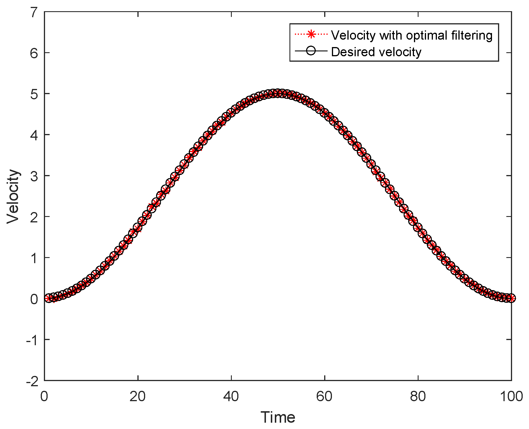
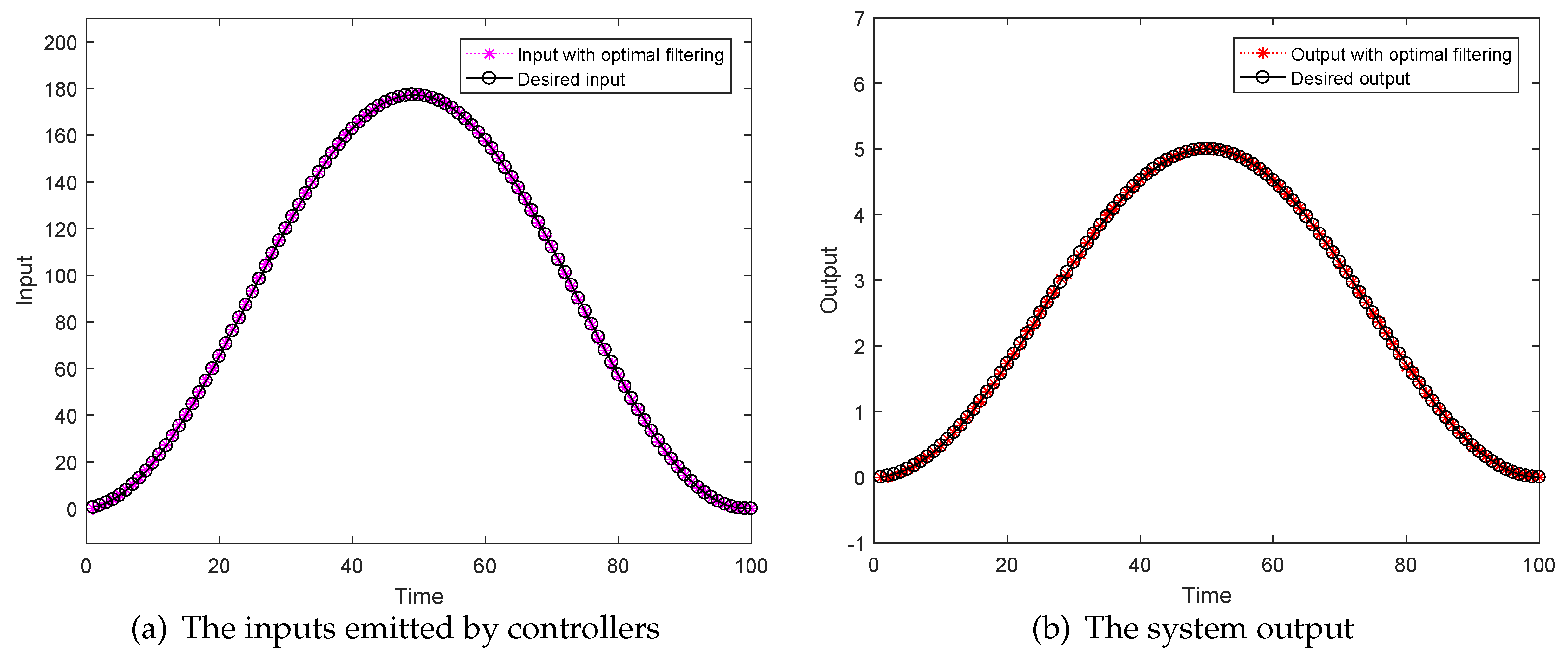
4. Simulation Results

Consider the velocity tracking of a direct current motor [35,36], the dynamic of which is represented as

$$\left\{\begin{array}{cc}\hfill \dot{x}\left(t\right)& =v\left(t\right)\hfill \\ \hfill u\left(t\right)& ={\displaystyle \frac{\pi }{\varsigma }}{\mathsf{\Psi }}_f\dot{x}\left(t\right)+Ri\left(t\right)+L\dot{i}\left(t\right)\hfill \\ \hfill f_d\left(t\right)& =M\dot{v}\left(t\right)+f_f\left(t\right)+f_r\left(t\right)+f_l\left(t\right)+f_d\left(t\right)\hfill \end{array}\right.$$

The definitions of motor parameters are provided in

Table 3. The definitions of parameters.

Parameter	Meaning	Parameter	Meaning
$x\left(t\right)$	motor position	$v\left(t\right)$	rotor velocity
$i\left(t\right)$	stator current	$u\left(t\right)$	stator voltage
${\mathsf{\Psi }}_f$	flux linkage	L	stator inductance
$f_f\left(t\right)$	frictional force	$f_d\left(t\right)$	developed force
$f_l\left(t\right)$	load force	$f_r\left(t\right)$	ripple force
$f_d\left(t\right)$	disturbances	R	stator resistance
$\varsigma$	pole pitch	M	rotor mass

.

According to the simplification steps in [35,36], the motor model can be rewritten as

$$\left\{\begin{array}{cc}\hfill \dot{x}\left(t\right)& =v\left(t\right)\hfill \\ \hfill \dot{v}\left(t\right)& =-{\displaystyle \frac{1.5{\pi }^2{\mathsf{\Psi }}_f^2}{{\varsigma }^{2}RM}}v\left(t\right)+{\displaystyle \frac{1.5\pi {\mathsf{\Psi }}_f}{\varsigma RM}}u\left(t\right)\hfill \\ \hfill y\left(t\right)& =v\left(t\right)\hfill \end{array}\right.$$

Using the Euler discretization and taking internal disturbances p and q into account, the simplified model is provided as

$$\left\{\begin{array}{cc}\hfill x(k+1)& =v\left(k\right)\delta +x\left(k\right)+0.3p\left(k\right)\hfill \\ \hfill v(k+1)& =-\delta {\displaystyle \frac{1.5{\pi }^2{\mathsf{\Psi }}_f^2}{{\varsigma }^{2}RM}}v\left(k\right)+v\left(k\right)+\delta {\displaystyle \frac{1.5\pi {\mathsf{\Psi }}_f}{RM}}u\left(k\right)+0.3p\left(k\right)\hfill \\ \hfill y\left(k\right)& =v\left(k\right)+0.5q\left(k\right)\hfill \end{array}\right.$$

(40)

where $M=1.635$ kg, R = 8.6 $\mathsf{\Omega }$, $\varsigma =0.031$ m, and ${\mathsf{\Psi }}_f=0.35$ Wb. It can be seen that the simplified model provided in Equation $\left(40\right)$ can be represented in the form provided in Equations $\left(1\right)$ and $\left(2\right)$, where $\underline{A}=\left[\begin{array}{cc}1& \delta \\ 0& 1-\delta {\displaystyle \frac{1.5{\pi }^2{\mathsf{\Psi }}_f^2}{{\varsigma }^{2}RM}}\end{array}\right]$, $\underline{B}=\left[\begin{array}{c}0\\ \delta {\displaystyle \frac{1.5\pi {\mathsf{\Psi }}_f}{RM}}\end{array}\right]$, $\underline{C}=\left[\begin{array}{c}0.3\\ 0.3\end{array}\right]$, $\underline{D}=\left[\begin{array}{c}0\\ 1\end{array}\right]$, and $\underline{H}=0.5$. The sampling interval $\delta$ is set to 0.01s, and each iteration cycle is 1s, meaning that $T=100$.

The expected velocity of the motor is provided as

$$y_d\left(k\right)=2.5\left(1+sin\left(2\pi k/\phantom{2\pi t100}\mathrm{T}\right)-\pi /\phantom{\pi 2}2\right)$$

The ILC strategy provided in $\left(3\right)$ is used with $\mathsf{\Gamma }\left(k\right)=0.9$. As a result, $∥I-\mathsf{\Gamma }\left(k\right)\underline{D}\underline{B}∥=0.6216<1$. The initial plant state and control input are set to 0, while p, q, m, and n are all zero mean with a variance of 0.05. Moreover, the delay probabilities are set as $\overline{\alpha }=\overline{\beta }=0.92$ and $\overline{\eta }=\overline{\xi }=0.96$, respectively. Additionally, the initial values used for state estimation are set as ${\widehat{X}}_l\left(0\right|-1)={\left[\begin{array}{cccc}1& 1& 1& \begin{array}{cc}1& 1\end{array}\end{array}\right]}^{\mathrm{T}}$ and $P_l\left(0\right|-1)=0.1I_5$, where $I_5$ is the 5-th order identify matrix. Additionally, to verify the effectiveness of the proposed estimation method, the time-domain compensation method in [37] is used as a benchmark.

Figure 2 illustrates the significant effects of random delay links on the velocity states of motors at the $30\mathrm{th}$ iteration. In contrast, Figure 3 demonstrates the velocity states of motors using the time-domain compensation method, demonstrating partial mitigation of the link effects. This is because this method is ineffective in dealing with mutual interference and noises both within and outside systems. Conversely, Figure 4 shows that the velocity states of motors are optimally estimated despite the effects of wireless delay links. This can be attributed to the established estimation model that comprehensively handles all uncertainties.

Figure 5 illustrates the inputs emitted by controllers and their corresponding outputs in the presence of effects of wireless delay links. This indicates that the emitted inputs fail to converge to the expected values after 30 iterations, leading to outputs that do not follow the expected trajectory. In contrast, Figure 6 shows the inputs emitted by the controller ends and the corresponding outputs with the compensation in the time domain. This figure indicates that the tracking capability of the emitted input is still insufficiently ensured, resulting in the output failing to converge to the expected trajectory. By comparison, Figure 7 demonstrates a significant improvement in the tracking capability of the inputs at the controller ends and the corresponding outputs due to the proposed state estimation method. This is because output errors used for controller learning are accurately obtained through state estimating. Consequently, the outputs produced by the inputs at the controller ends converge to the desired outputs.

Figure 8, Figure 9, Figure 10, Figure 11, Figure 12 and Figure 13 show the velocity states of the motors, inputs emitted by the controllers, and their corresponding outputs under three comparison methods when the four noise variances increase to 0.15. Compared with the system convergence curves at the variance of 0.05, it is observed that the increase in variance causes larger fluctuations in the convergence curves generated by the two benchmark methods. However, this paper’s proposed estimator still enables the system output to accurately track the desired velocity trajectory. Figure 14, Figure 15 and Figure 16 further present the tracking accuracy using the mean absolute errors of the system states, the inputs emitted by the controller ends, and the outputs generated by those inputs when the four variances are 0.15. Since the output is the motor velocity under the influence of the internal disturbance variable q, the output convergence curve under unprocessed conditions is very similar to the motor velocity convergence curve. Moreover, it is worth emphasizing that the compensation method only marginally improves the tracking accuracy of this system. In contrast, the estimation method introduced in this paper markedly improves the tracking accuracy, further validating the validity of the developed estimation method.

5. Conclusions

This paper focuses on the precise tracking of plants implementing ILC strategies through wireless delay links. To cope with the challenges posed by noisy links, a data pre-processing method is designed to ensure that the controllers or actuators receive only one piece of data at each time instant. Subsequently, the system information and the designed pre-processing method are utilized to establish an estimation model, and a state estimator based on the theory of orthogonality is proposed. Using the proposed state estimator, the true outputs are derived for controller learning to improve the system tracking accuracy.

It is worth highlighting that the proposed state estimation method depends on the assumptions about the mean and variance of the system disturbances and link noises. As a future step, we plan to develop robust state estimators and explore extending the proposed estimation method for multi-agent systems.

References

1. Zhang, X.; Han, Q.; Ge, X.; Ding, D.; Ding, L.; Yue, D.; Peng, C. Networked control systems: A survey of trends and techniques. IEEE/CAA J. Autom. Sin. 2019, 7, 1–17. [Google Scholar] [CrossRef]
2. Li, M.; Chen, Y. Challenging research for networked control systems: A survey. Trans. Inst. Meas. Control 2019, 41, 2400–2418. [Google Scholar] [CrossRef]
3. Mahmoud, M.S.; Hamdan, M.M. Fundamental issues in networked control systems. IEEE/CAA J. Autom. Sin. 2018, 5, 902–922. [Google Scholar] [CrossRef]
4. Wang, Y.; Han, Q. Network-based modelling and dynamic output feedback control for unmanned marine vehicles in network environments. Automatica 2018, 91, 43–53. [Google Scholar] [CrossRef]
5. Ding, L.; Han, Q.; Wang, L.Y.; Sindi, E. Distributed cooperative optimal control of DC microgrids with communication delays. IEEE Trans. Ind. Inf. 2018, 14, 3924–3935. [Google Scholar] [CrossRef]
6. Sandberg, H.; Amin, S.; Johansson, K.H. Cyberphysical security in networked control systems: An introduction to the issue. IEEE Control Syst. Mag. 2015, 35, 20–23. [Google Scholar]
7. Hespanha, J.P.; Naghshtabrizi, P.; Xu, Y. A survey of recent results in networked control systems. Proc. IEEE 2007, 95, 138–162. [Google Scholar] [CrossRef]
8. Fu, X.; Peng, J. Iterative learning control for UAVs formation based on point-to-point trajectory update tracking. Math. Comput. Simul. 2023, 209, 1–15. [Google Scholar] [CrossRef]
9. Sanzida, N.; Nagy, Z.K. Iterative learning control for the systematic design of supersaturation controlled batch cooling crystallisation processes. Comput. Chem. Eng. 2013, 59, 111–121. [Google Scholar] [CrossRef]
10. Chen, D.; Xu, Y.; Lu, T.; Li, G. Multi-phase iterative learning control for high-order systems with arbitrary initial shifts. Math. Comput. Simul. 2024, 216, 231–245. [Google Scholar] [CrossRef]
11. Feng, X.; Zhang, Y.; Kang, L.; Wang, L.; Duan, C.; Yin, K.; Pang, J.; Wang, K. Integrated energy storage system based on triboelectric nanogenerator in electronic devices. Front. Chem. Sci. Eng. 2021, 15, 238–250. [Google Scholar] [CrossRef]
12. Zhou, M.; Wang, J.; Shen, D. Iterative learning based consensus control for distributed parameter type multi-agent differential inclusion systems with time-delay. Comput. Math. Appl. 2022, 127, 25–47. [Google Scholar] [CrossRef]
13. Lv, Y.; Chi, R.; Feng, Y. Adaptive estimation-based TILC for the finite-time consensus control of non-linear discrete-time MASs under directed graph. IET Control Theory Appl. 2018, 12, 2516–2525. [Google Scholar] [CrossRef]
14. Hui, Y.; Chi, R.; Huang, B.; Hou, Z. Extended state observer-based data-driven iterative learning control for permanent magnet linear motor with initial shifts and disturbances. IEEE Trans. Syst. Man Cybern. Syst. 2019, 51, 1881–1891. [Google Scholar] [CrossRef]
15. Wang, Y.; Zhao, Z.; Ge, C.; Wang, L.; Liu, Y. Networked control systems with probabilistic time-varying delay based on event-triggered non-fragile H control. Math. Comput. Simul. 2022, 202, 206–222. [Google Scholar] [CrossRef]
16. Pan, Y.; J Marquez, H.; Chen, T.; Sheng, L. Effects of network communications on a class of learning controlled non-linear systems. Int. J. Syst. Sci. 2009, 40, 757–767. [Google Scholar] [CrossRef]
17. Huang, L.; Sun, L.; Wang, T.; Liu, W.; Zhang, Z.; Zhang, Q. Optimal input filters for iterative learning control systems with additive noises, random delays, and data dropouts in both channels. Math. Methods Appl. Sci. 2022, 45, 4295–4311. [Google Scholar] [CrossRef]
18. Huang, L.; Sun, L.; Chen, T.; Zhang, Q.; Huo, L.; Liu, W. Input predictors for networked iterative learning control systems with data dropouts and time delays. J. Intell. Fuzzy Syst. 2023, 45, 3333–3344. [Google Scholar] [CrossRef]
19. Shen, D.; Zhang, C.; Xu, Y. Intermittent and successive ILC for stochastic nonlinear systems with random data dropouts. Asian J. Control 2018, 20, 1102–1114. [Google Scholar] [CrossRef]
20. Zhang, Y.; Liu, J.; Ruan, X. Iterative learning control for uncertain nonlinear networked control systems with random packet dropout. Int. J. Robust Nonlinear Control 2019, 29, 3529–3546. [Google Scholar] [CrossRef]
21. Shen, D.; Wang, Y. Iterative learning control for networked stochastic systems with random packet losses. Int. J. Control 2015, 88, 959–968. [Google Scholar] [CrossRef]
22. Shen, D.; Wang, Y. ILC for networked nonlinear systems with unknown control direction through random lossy channel. Syst. Control Lett. 2015, 77, 30–39. [Google Scholar] [CrossRef]
23. Shen, D.; Xu, J. A novel markov chain based ILC analysis for linear stochastic systems under general data dropouts environments. IEEE Trans. Autom. Control 2016, 62, 5850–5857. [Google Scholar] [CrossRef]
24. Shen, D.; Jin, Y.; Xu, Y. Learning control for linear systems under general data dropouts at both measurement and actuator sides: A markov chain approach. J. Franklin Inst. 2017, 354, 5091–5109. [Google Scholar] [CrossRef]
25. Bu, X.; Yu, F.; Hou, Z.; Wang, F. Iterative learning control for a class of nonlinear systems with random packet losses. Nonlinear Anal. Real World Appl. 2013, 14, 567–580. [Google Scholar] [CrossRef]
26. Sun, S. Linear optimal state and input estimators for networked control systems with multiple packet dropouts. Int. J. Innov. Comput I 2012, 8, 7289–7305. [Google Scholar]
27. Huang, L.; Zhang, Q.; Liu, W.; Li, J.; Sun, L.; Wang, T. Convergence analysis of iterative learning control systems over networks with successive input data compensation in iteration domain. IEEE Access 2019, 7, 160217–160226. [Google Scholar] [CrossRef]
28. Liu, J.; Ruan, X. Synchronous-substitution-type iterative learning control for discrete-time networked control systems with bernoulli-type stochastic packet dropouts. IMA J. Math. Control Inf. 2018, 35, 939–962. [Google Scholar] [CrossRef]
29. Hao, G.; Sun, S. Distributed fusion filter for nonlinear multi-sensor systems with correlated noises. IEEE Access 2020, 8, 39548–39560. [Google Scholar] [CrossRef]
30. Huang, L.; Sun, L.; Wang, T.; Zhang, Q.; Liu, W.; Zhang, Z. An optimal filter for updated input of iterative learning controllers with multiplicative and additive noises. Int. J. Syst. Sci. 2022, 53, 1516–1528. [Google Scholar] [CrossRef]
31. Liu, W.; Chi, R. Iterative learning control for nonlinear nonaffine networked systems with stochastic noise in communication channels. Trans. Inst. Meas. Control 2021, 43, 3158–3168. [Google Scholar] [CrossRef]
32. Lai, J.; Xiong, J.; Shu, Z. Model-free optimal control of discrete-time systems with additive and multiplicative noises. Automatica 2023, 147, 110685. [Google Scholar] [CrossRef]
33. Huang, L.; Sun, L.; Wang, T.; Zhang, Q.; Li, J.; Zhang, Z.; Liu, W. Optimal input filtering for networked iterative learning control systems with packet dropouts and channel noises in both sides. Int. J. Robust Nonlinear Control 2022, 32, 5086–5104. [Google Scholar] [CrossRef]
34. Anderson, B.D.; Moore, J.B. Optimal Filtering; Courier Corporation: North Chelmsford, MA, USA, 1979. [Google Scholar]
35. Shen, D.; Zhang, C.; Xu, Y. Two updating schemes of iterative learning control for networked control systems with random data dropouts. Inf. Sci. 2017, 381, 352–370. [Google Scholar] [CrossRef]
36. Zhou, W.; Yu, M.; Huang, D. A high-order internal model based iterative learning control scheme for discrete linear time-varying systems. Int. J. Autom. Comput. 2015, 12, 330–336. [Google Scholar] [CrossRef]
37. Liu, J.; Ruan, X. Networked iterative learning control design for discrete-time systems with stochastic communication delay in input and output channels. Int. J. Syst. Sci. 2017, 48, 1844–1855. [Google Scholar] [CrossRef]
Figure 1. Plants implementing ILC strategies with state estimators.
Mathematics 12 02834 g001
Figure 2. The velocity states of motors with no processing when noise variances are 0.05.
Mathematics 12 02834 g002
Figure 3. The velocity states of motors with the time-domain compensation when noise variances are 0.05.
Mathematics 12 02834 g003
Figure 4. The velocity states of motors with the proposed estimator when noise variances are 0.05.
Mathematics 12 02834 g004
Figure 5. The inputs emitted by controllers and corresponding outputs with no processing when noise variances are 0.05.
Mathematics 12 02834 g005
Figure 6. The inputs emitted by controllers and corresponding outputs with the time-domain compensation when noise variances are 0.05.
Mathematics 12 02834 g006
Figure 7. The inputs emitted by controllers and corresponding outputs with the proposed estimator when noise variances are 0.05.
Mathematics 12 02834 g007
Figure 8. The velocity states of motors with no processing when noise variances are 0.15.
Mathematics 12 02834 g008
Figure 9. The velocity states of motors with the time-domain compensation when noise variances are 0.15.
Mathematics 12 02834 g009
Figure 10. The velocity states of motors with the proposed estimator when noise variances are 0.15.
Mathematics 12 02834 g010
Figure 11. The inputs emitted by controllers and corresponding outputs with no processing when noise variances are 0.15.
Mathematics 12 02834 g011
Figure 12. The inputs emitted by controllers and corresponding outputs with the time-domain compensation when noise variances are 0.15.
Mathematics 12 02834 g012
Figure 13. The inputs emitted by controllers and corresponding outputs with the proposed estimator when noise variances are 0.15.
Mathematics 12 02834 g013
Figure 14. The convergence of mean absolute errors of velocity states of motors when noise variances are 0.15.
Mathematics 12 02834 g014
Figure 15. The convergence of mean absolute errors of inputs emitted by controllers when noise variances are 0.15.
Mathematics 12 02834 g015
Figure 16. The convergence of mean absolute errors of system output when noise variances are 0.15.
Mathematics 12 02834 g016