

A Sustainable Supply Chain Model with Variable Production Rate and Remanufacturing for Imperfect Production Inventory System under Learning in Fuzzy Environment


Abstract
:1. Introduction
2. Literature Review
2.1. Literature Related to the Flexible Production of Inventory
2.2. Literature Related with Remanufacturing and Defective Items
2.3. Literature Related with Optimized Backorder
2.4. Literature Related to Environmental Issues
2.5. Literature Related to Fuzzy and Learning in Environment
2.6. Research Gap and Proposed Work
2.7. Novelty and Research Contribution of Our Proposed Work
- The lack of learning fuzzy theory in the previous research work is completed with the help of this proposed model and the total inventory fuzzy cost is minimized using learning fuzzy theory. This approach is more and more beneficial for the cost reduction policy in the field of the production of electronic products.
- A lot of authors have developed an inventory model with a fuzzy environment under different approaches and have not considered the concept of learning in a fuzzy environment while the proposed model considers the concept of learning in a fuzzy environment and calculates the total fuzzy cost under learning in a fuzzy environment where left and right deviation in fuzzy demand follow the effect of learning.
- The suggested approach considers a flexible production system to close the aforementioned research gap. A key tactic for effectively enhancing market responsibility in the face of future demand uncertainty despite any shortages is to increase flexibility in production. Different product types might be built simultaneously in the same production facility thanks to flexible manufacturing.
- This model is intended for product assembly from multiple parts to meet the various needs of customers. Consumer expectations are continually linked to a product variation based on their personal preferences (this paper examines a particular electronic product). This need can only be met and the system profit raised by a merchandise assembly method built on a flexible production system.
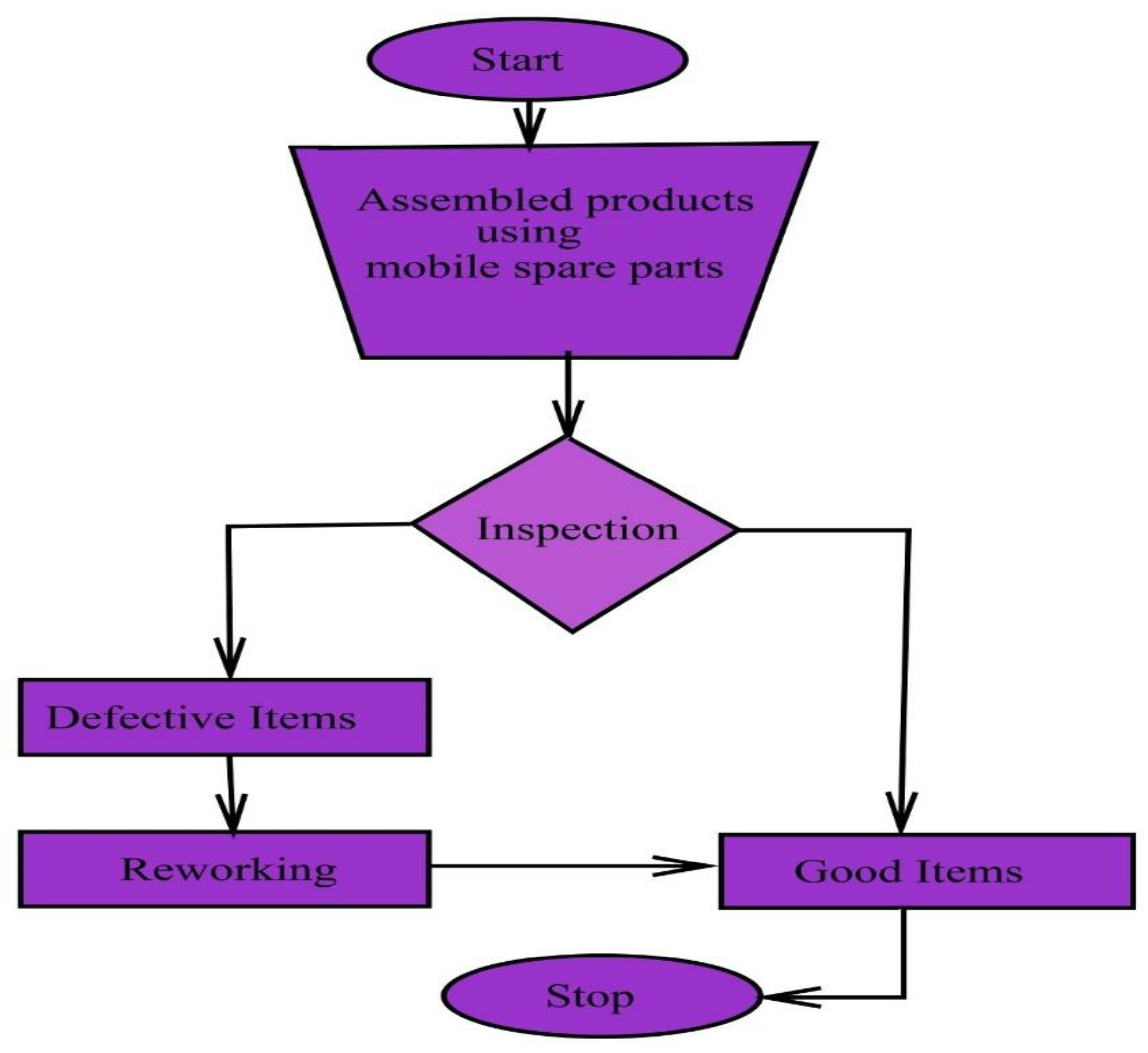
- The suggested model applies an inspection strategy to prevent a defective final product. The production system will obtain significant monetary profit from this approach. Once a product is sold, the model lowers end-user backorders of goods after production but before being sold to the final consumer, the inspection strategy for defective assembled products is carried out, and the defective products are sent to be recycled.
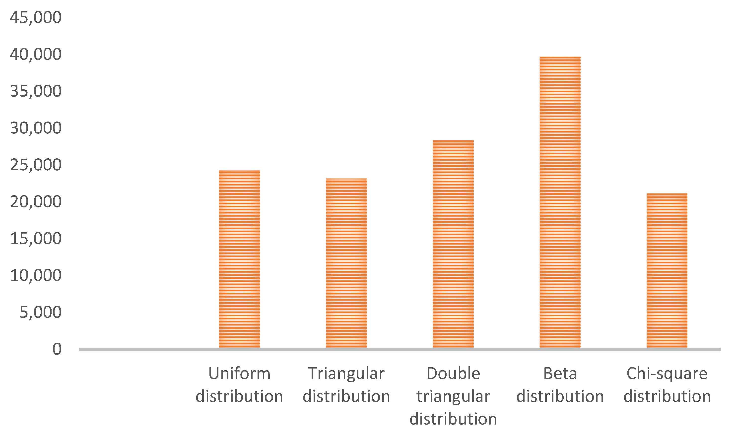
- The role of statistical distributions in the field of the business sector is more applicable to the reduction in cost function. In this paper, we selected five types of statistical distributions, namely, uniform, triangular, beta (β), double-triangular probability distributions, and χ2 (chi−square). It is assumed that the percentage of defective items follows these distributions and the total fuzzy cost varies concerning each distribution with its expected values. We calculate the total fuzzy cost under each distribution with its expected values and after that, we compare the total fuzzy cost under these distributions. For the sensitivity analysis, we select that distribution in which the total fuzzy cost is minimum and such distribution is more applicable for the proposed model and other input parameters receive a positive response on the total inventory fuzzy cost.
- Remanufacturing policies have the potential to recover defective products prior to sale and decrease the amount of end-user backorders. There has not been any prior research on this flexible production system research gap in the literature. The total fuzzy cost is minimum in the χ2 distribution as compared to uniform, triangular, beta (β), and double-triangular probability distributions. This tactic can increase the system’s financial gains. Increasing sales and satisfying end-user demands are critical to a production system’s financial success. An industry can respond to end users more quickly by implementing flexible production. This study’s contribution is in the form of a mathematical model with a changeable rate of production for one type of item.
- Concern for practically all products, including electronic products, as they suggest that the inventory of work-in-process is under control. This is so that even though the process of supplying a product is dependent upon market demand, the production of any product can be predicted. The just-in-time production policy is used in this study to examine an inspection policy for product assembly. This policy, which is more successful than the conventional method of inspection, delivers all imperfect quality items for remanufacturing of imperfect quality items before selling the final goods to the end operators. This can help reduce wasteful spending, boost sales, and improve the overall profit. If defective items need to be remanufactured after they are made ready for sale, this method benefits industries by lowering the costs of holding space. As a result, with flexible and economical production, less waste is generated in the form of defective products. The quality of the final assembled products can be raised by managing the remanufacturing of defective products under flexible production. Moreover, boosting production flexibility will stop shortages from occurring as a result of smart production. Remanufacturing products helps reduce returns, which is a significant financial benefit for industries. If this were not the case, they might have to pay high maintenance costs for the vast majority of products that end users return.
2.8. Organization of Proposed Plan
3. Notations and Assumptions
3.1. Notations
- -
- : The number of batches to production a single amassed items where,
- -
- : Production rate for j products (units per time) (decision variable);
- -
- : The production lot for j products (units per cycle) (decision variable);
- -
- : The number of shortages lot size for j products (units) (decision variable);
- -
- : The rate of order of j products (units per time);
- -
- : The shipment expenses of j products (USD per shipment);
- -
- : The manufacturing costs of j products (USD per unit);
- -
- : The carrying cost for j product (USD per unit per time);
- -
- : The linear shortage costs for j products (USD per unit per time);
- -
- : The lot number (in integers);
- -
- : The backorder cost for fixed shortages j product/backorder (USD per backorder);
- -
- : The average backorder of item j (units);
- -
- : Cycle length (time units);
- -
- : The whole inventory cost (units);
- -
- : The whole inventory cost per unit time (units);
- -
- : The remanufacturing costs for products (USD per item);
- -
- : The budget of j products (units);
- -
- : The volume for storage of products (units);
- -
- : Whole amount of budget (in USD);
- -
- : The regular inventory for (units);
- -
- : Maximum inventory level where, (units);
- -
- : The rate of fuzzy demand of item j (units per time);
- -
- : The lower deviation of fuzzy demand of item j (units per time);
- -
- : The upper deviation of fuzzy demand of item j (units per time);
- -
- : The whole fuzzy inventory cost per unit time (units);
- -
- : The whole fuzzy inventory cost per unit time (units) under learning in fuzzy environment;
- -
- : The slope of learning input parameter;
- -
- : The random percentage imperfect quality products in each cycle;
- -
- : Expected percentage of imperfect products ;
- -
- Stands for distribution;
- -
- Stands for ;
- -
- Stands for double–triangular distribution;
- -
- Stands for
- -
- Stands for which represents not feasible.
3.2. Assumptions
- ➢
- In the model, we are assuming a single assembled item is manufactured during the production of items. An electronic product is an example of a single assembled product and is prepared from different electronic parts j which depends on the customer’s demand. The various components are sold individually from different warehouses. The effects of product assembly in a market with competition are the main topic of this study. A fuzzy demand under flexible production can be promptly satisfied without causing any displeasure to the customer.
- ➢
- The production rate in this model is constantly higher than the fuzzy demand and is variable. According to Alexopoulos et al. [12], the model’s entire inventory system is predicated on an unlimited scheduling horizon under changeable manufacture, and it is feasible to determine the deepest manufacture inventory price under an unlimited time distance.
- ➢
- Following production, every assembled product is examined, and any issues are promptly reported for remanufacturing so that the same production cycle can continue.
- ➢
- Each product has a fixed inspection cost, although since it is much less than the other costs, it is adjusted based on setup costs. According to Dey et al. [25], the imperfect rate of imperfect items under variable production was permitted to be accidental. As a result, five distinct distribution functions (uniform, triangular, double-triangular, beta, and 𝜒2) are used to evaluate the optimal fuzzy cost individually under learning in a fuzzy environment.
- ➢
- After selling the completed assembled products, the model first experiences shortages, but all of these are fully backlogged. No sales are lost. There are two different kinds of backorder costs in this model: fixed backorder costs, which apply to the maximum backorder level, and linear backorder costs, which apply to average backorders during fuzzy environment and also the concept of average inventory, changeable production, limitations of budget, space for holding items, and other assumptions are taken from (Sarkar et al. [5]).
- ➢
- The production of a single product assembled from various components is examined in this paper. The objective of this model in a flexible production system is to minimize inventory costs under learning in a fuzzy environment and damage to the assembled product while taking the constraints of budget and space capacity into account. The model incorporates random defective rates and multi-item clean production, building upon the benchmark model of Carreras-Barron [4] during a fuzzy environment.
- ➢
- It is also considered that the effect of learning is involved in the lower and upper fuzzy range of customer’s demand.
- ➢
- Carbon emissions come from the storage of holding units and carbon emission costs are included in this manuscript.
4. Mathematical Formulation
4.1. Problem Definition
4.2. Formulation of the Proposed Model
4.3. Formulation of Crisp Model under Fuzzy Environment
4.4. Formulation of the Proposed Model under Learning Fuzzy Environment

4.5. Financial Plan and Space Limitations
5. Solution Method


Numerical Example
6. Discussion of Our Study with Previous Contributions
7. Sensitivity Analysis
- ➢
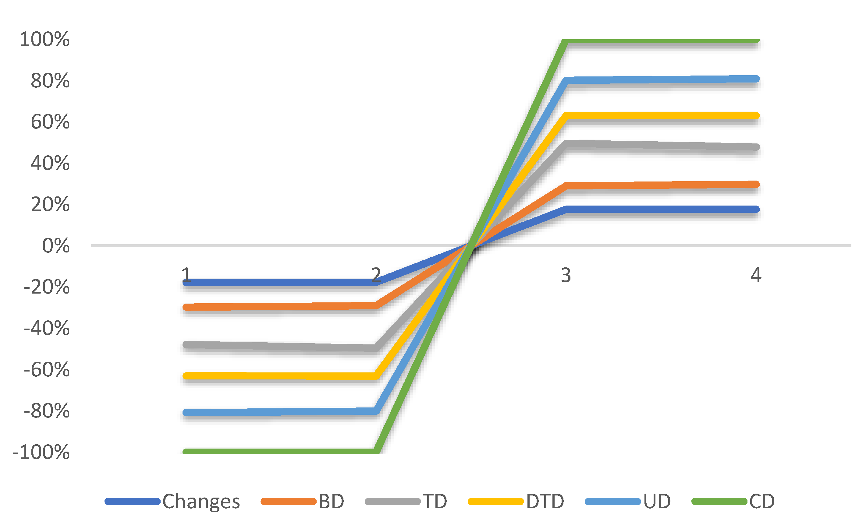
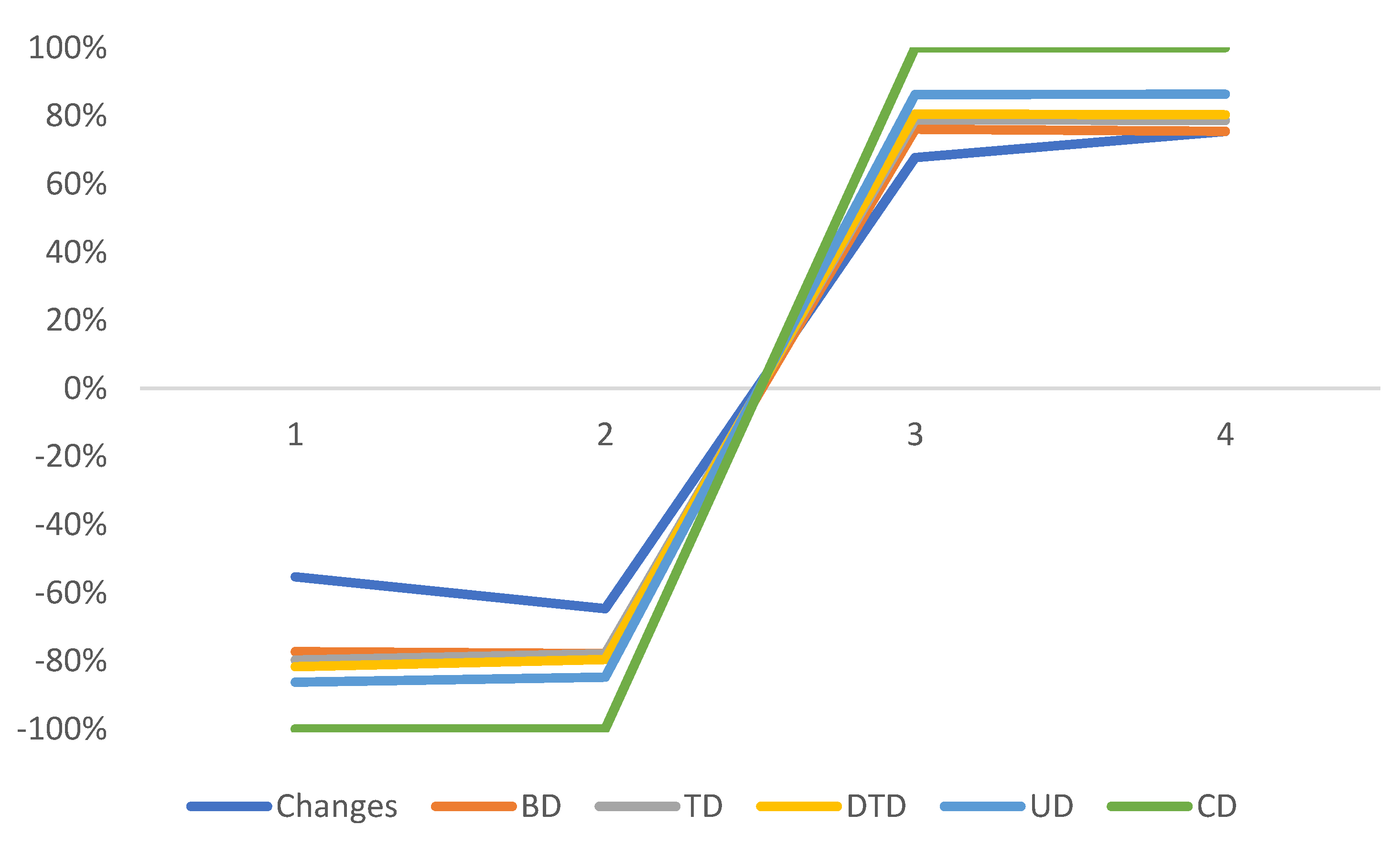
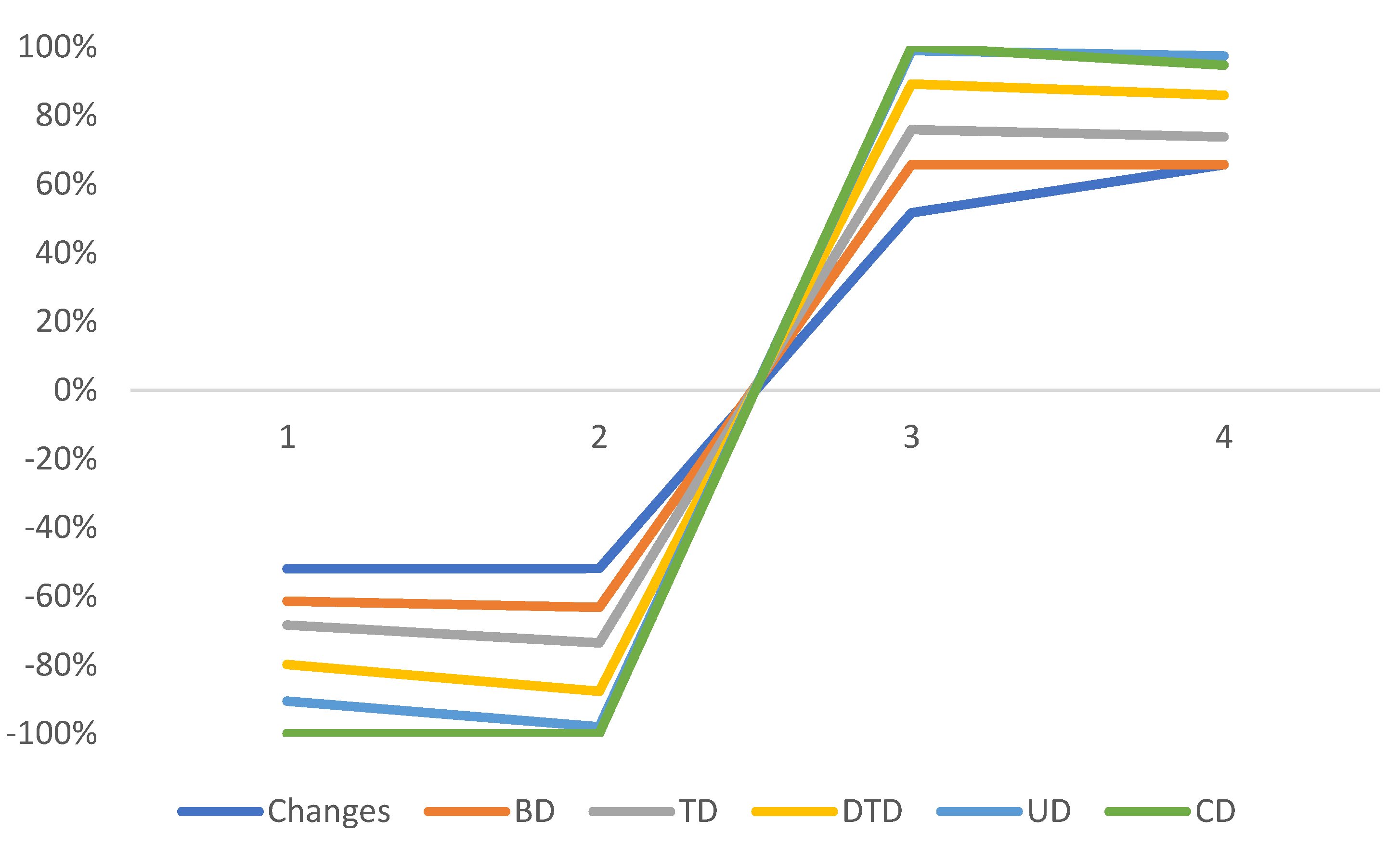
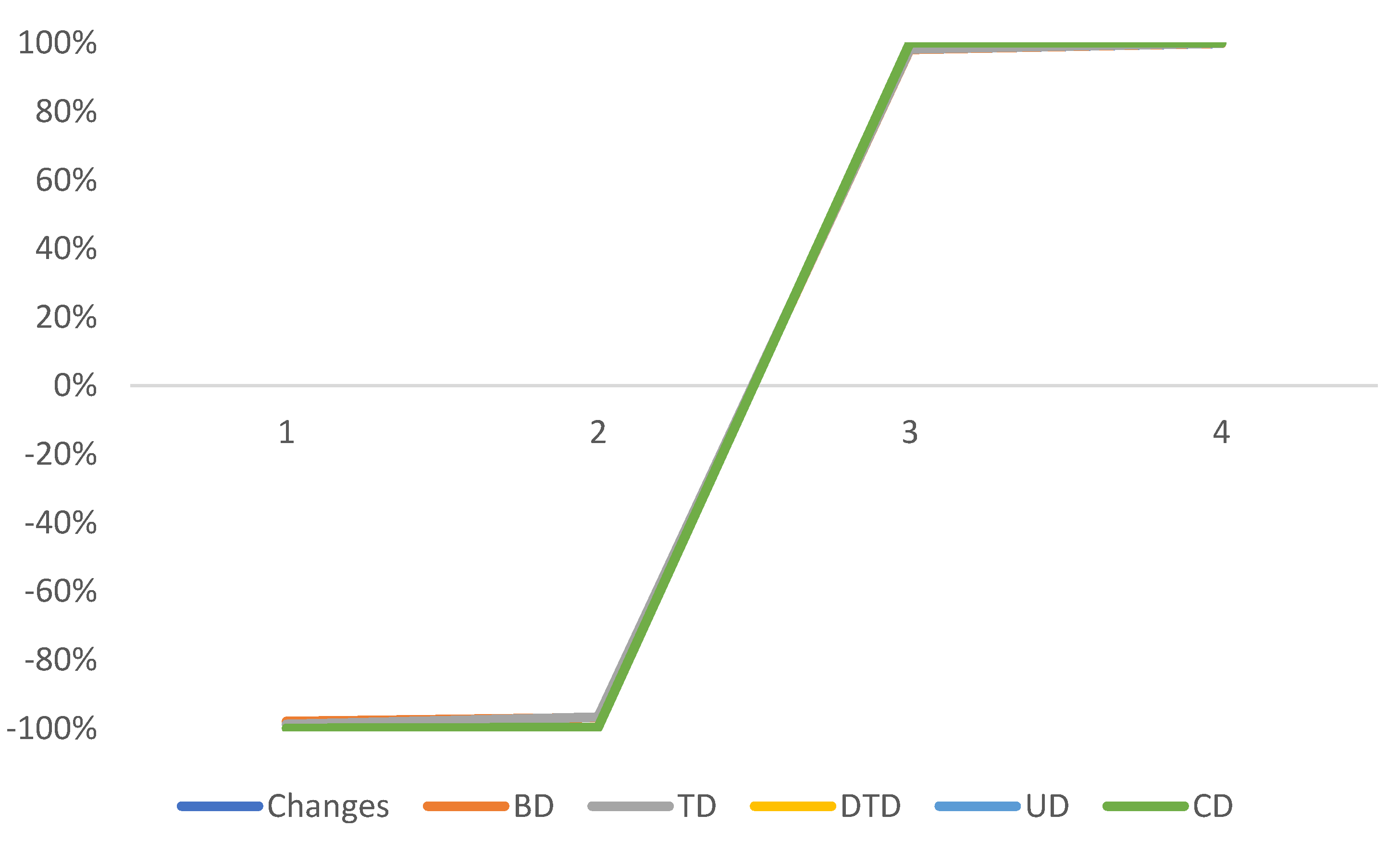
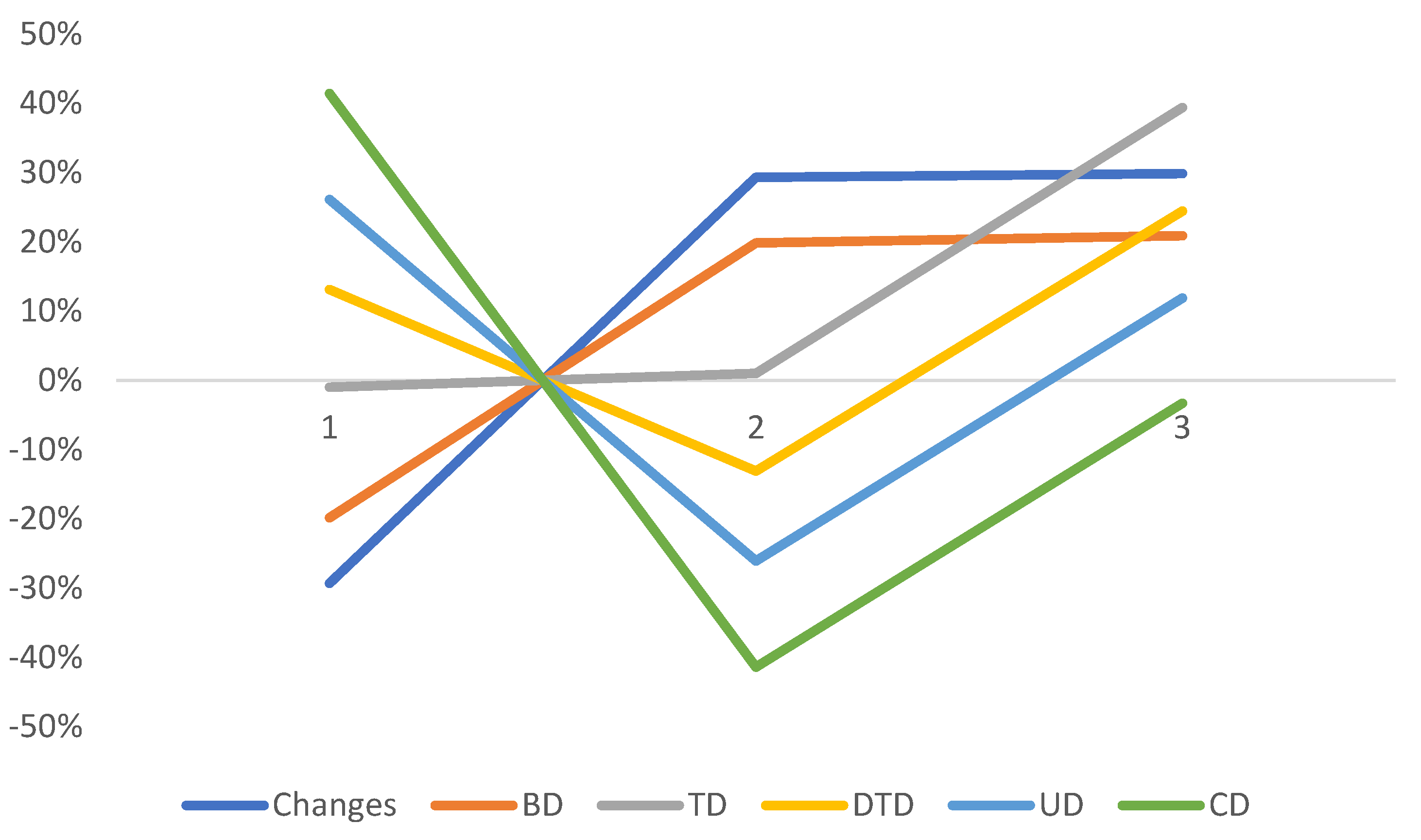
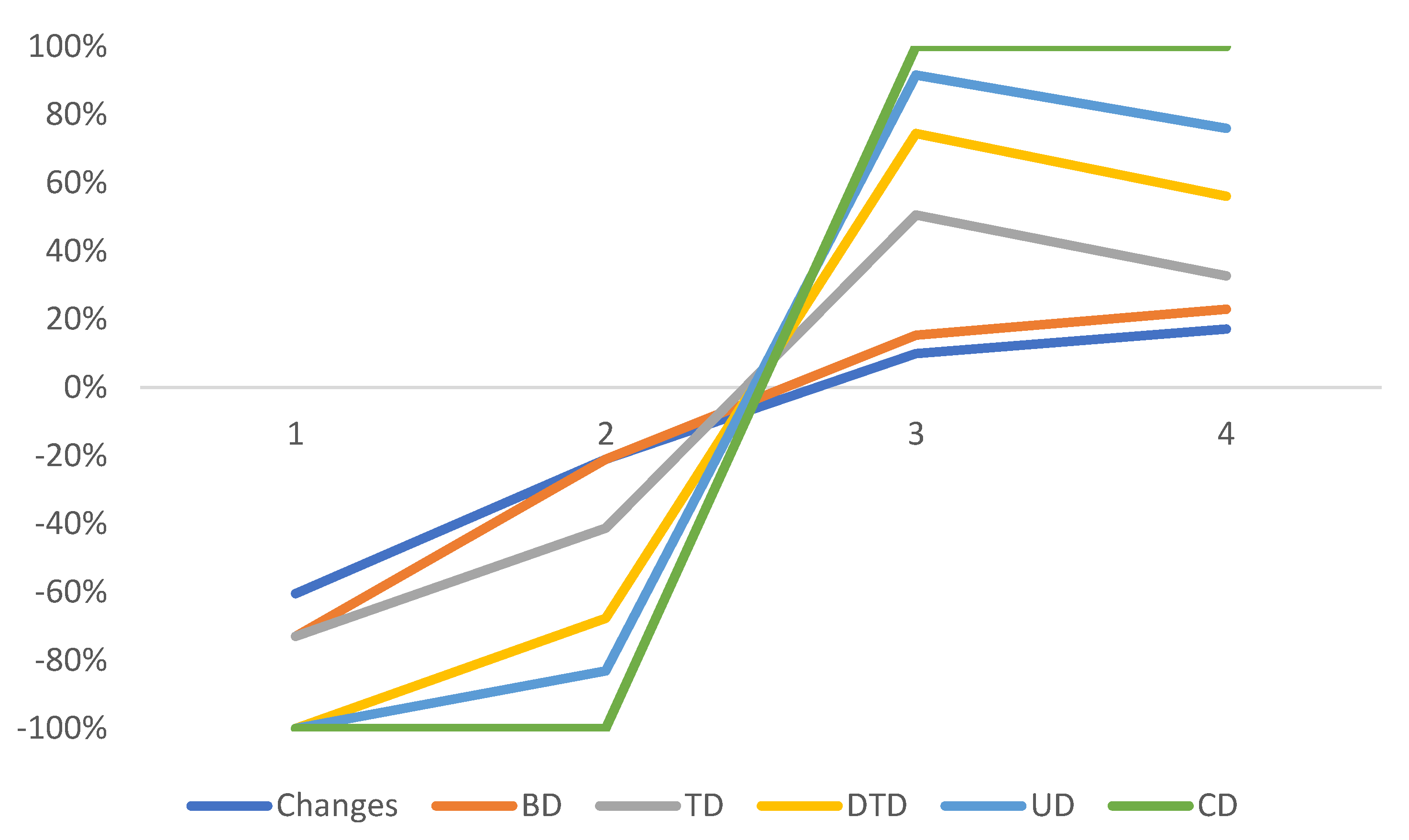
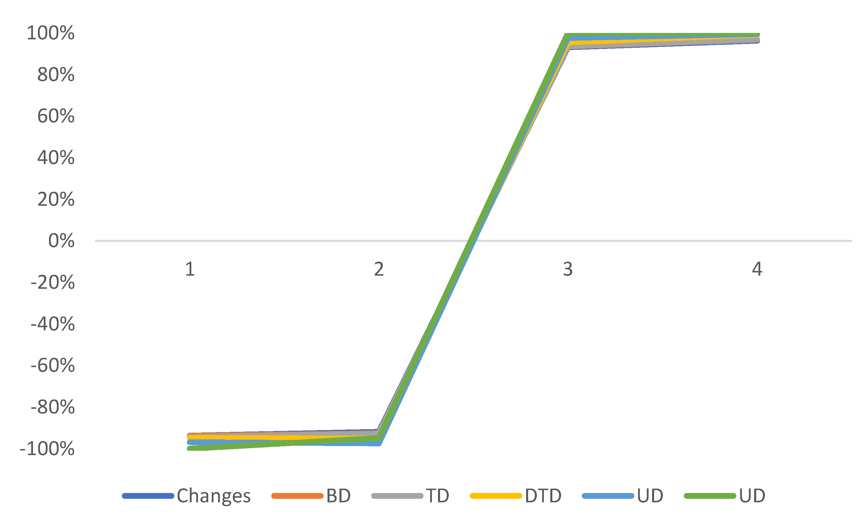
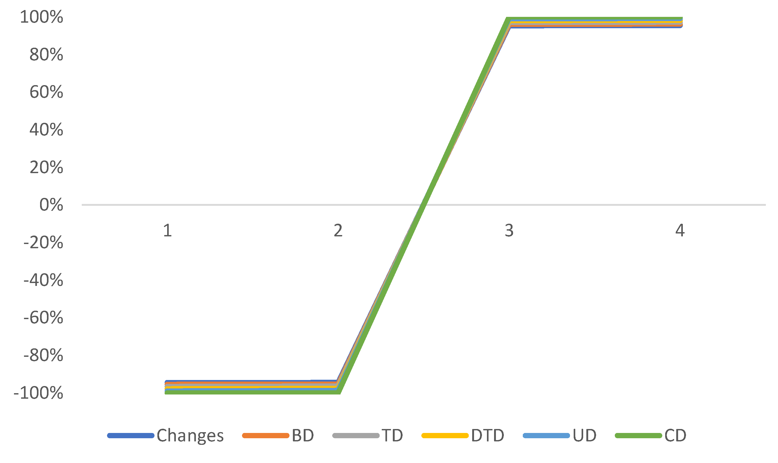
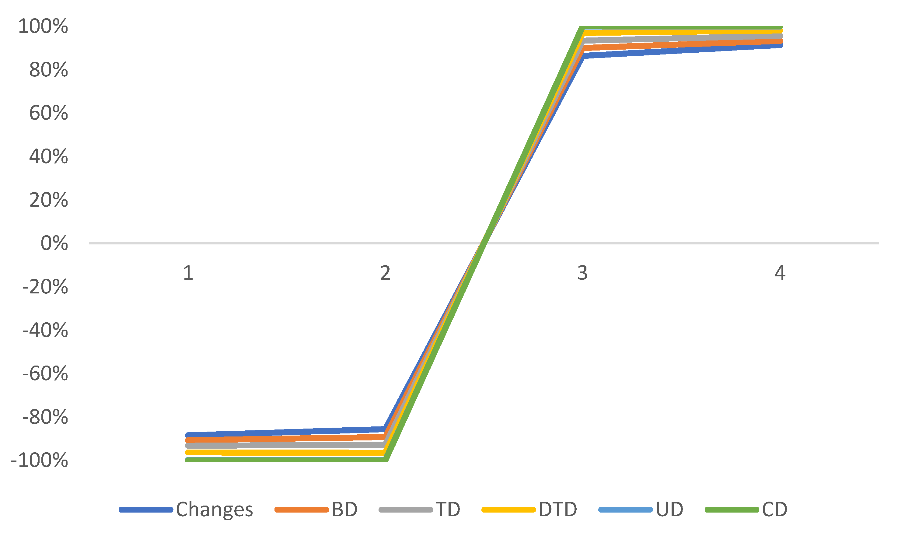
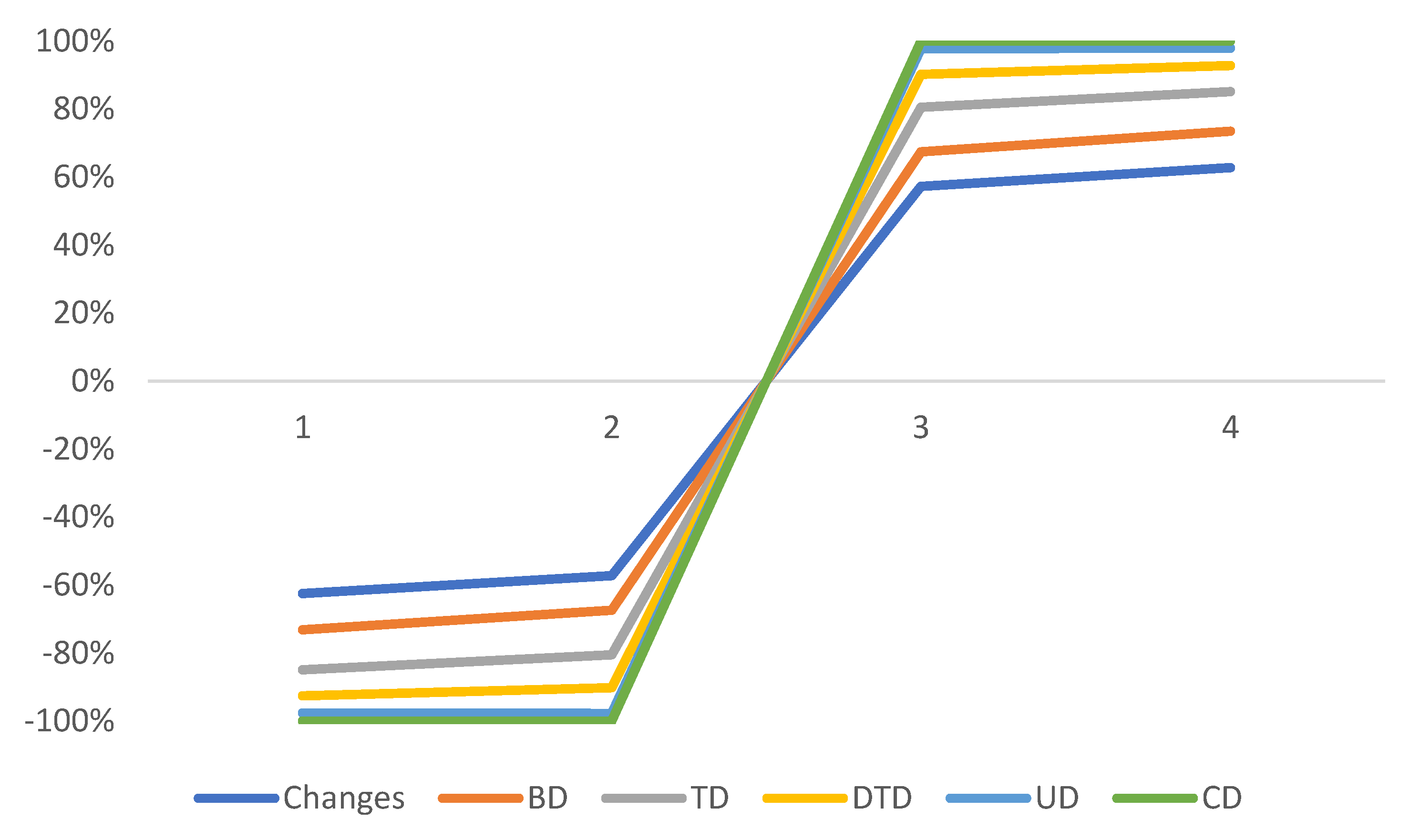
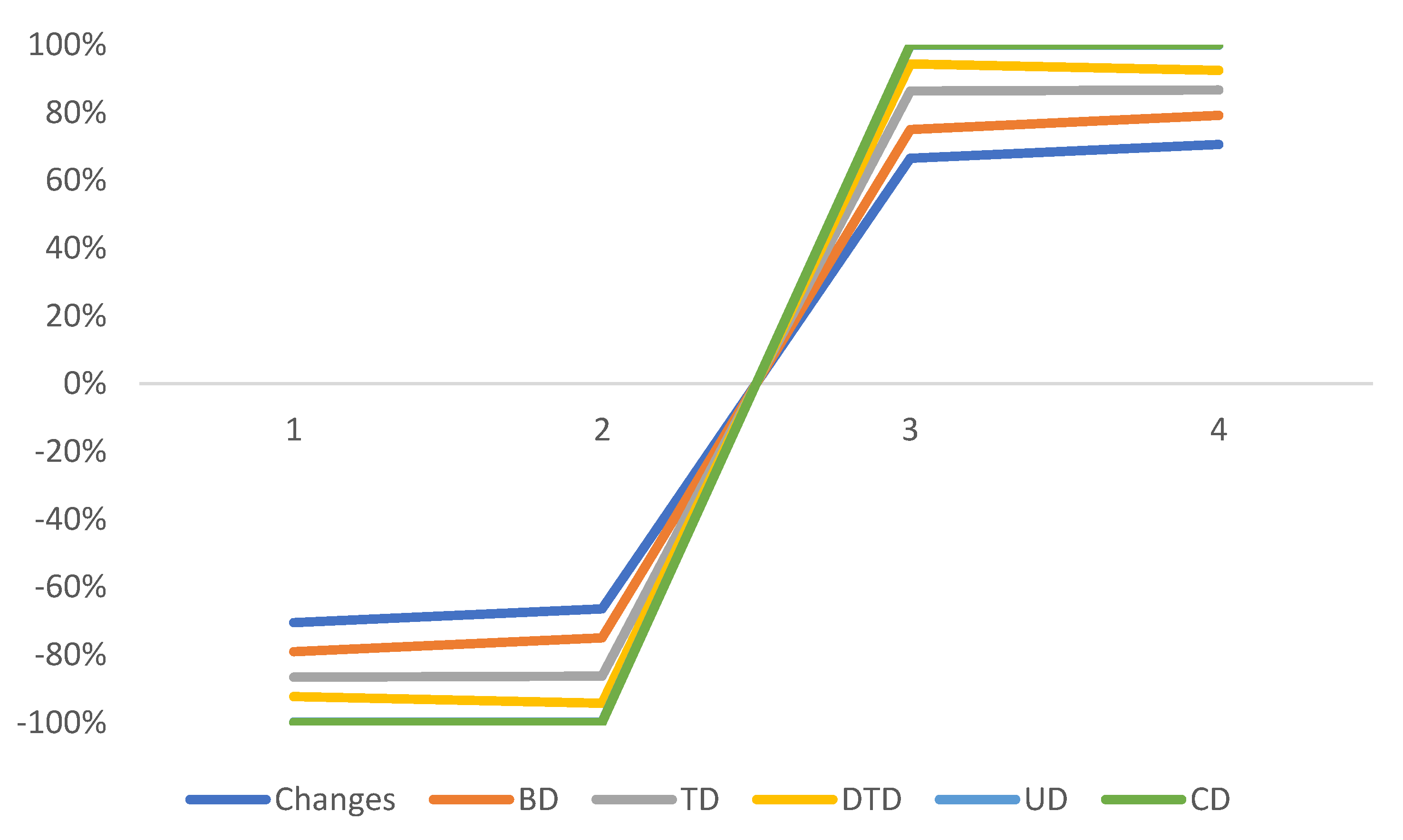
- The variation in the value of with both negative and negative from −50% to +50% means then the total inventory fuzzy cost is directly affected by the change in the values of . In the observations, the value of parameter and is more and more effective under the -distribution and χ2-distribution. From Table 9, the inventory input has a smaller effect on the value of total inventory fuzzy cost than the other parameters.
- ➢
- In this model, the budget and space restrictions with corresponding modifications are more delicate. Table 9 shows that both constraints consistently affect the overall total inventory fuzzy cost.
- ➢
- The manufacturing cost, carbon effect and holding cost are the two parameters that change significantly with both positive and negative changes. Additionally, each distribution has a negative sign, suggesting that the two parameters’ changes have little effect on the overall cost.
- ➢
- At each stage of the distributions, there are small adjustments made to the setup cost, linear backorder cost, and fixed backorder cost parameters within the −50% to 50% range. Consequently, these small adjustments have an impact on the overall cost, showing that the total inventory fuzzy cost varies with different distributions.
- ➢
- If we change with both negative and positive values of learning rates from −50% to +50%, then each distributions are varying according to the variation in learning rates with different numerical values but distribution has less value others distribution. If the rate of learning increases from −60% to +60%, then the value of distribution remains constant and the distribution of others varies with respect to the learning rate. Due to variation in the distribution of others with respect to the learning rate, the total fuzzy cost also varies. Finally, the total fuzzy cost remains cost under distribution if the rate of learning increases from −60% to +60%. It means that distribution is more beneficial for this proposed model. The total inventory fuzzy cost is minimized when the rate of learning achieves the position of saturation. If the decision-makers take the values of the learning rate in the form of a percentage from −60% to +60%, then the total fuzzy cost can be expected under such assumption. The concept of the learning theory gave positive effect in this model and is also applicable for the reduction in cost function.
- ➢
- If we change the value of the upper and lower deviation of the fuzzy demand rate and then distribution has less value than the distribution of others and it means that the distribution is more beneficial for this proposed model. The total inventory fuzzy cost is minimized when distribution is allowed for this proposed model.
8. Conclusions and Future Work
8.1. Uniqueness of Our Proposed Model
8.2. Application of Our Proposed Model
8.3. Social Implications of Our Proposed Model
8.4. The Implications of Our Proposed Model in the Waste Management Policy
8.5. Limitations of Our Proposed Model
- ➢
- The present proposed model is beneficial for the production of electronic items not for ordering policies.
- ➢
- The variation in fuzzy input parameters should be according to the proposed study.
- ➢
- The values of learning inputs should be according to the proposed model.
- ➢
- The deviations of fuzzy demand, namely lower and upper, should be according to the proposed model.
- ➢
- The financial plan and budget constraints should be allowed.
Funding
Data Availability Statement
Conflicts of Interest
Appendix A
- (i)
- Set-up cost (with inspection cost):
- (ii)
- Manufacturing cost:
- (iii)
- Inventory holding cost:
- (iv)
- Backordering cost:
- (v)
- Remanufacturing cost:
- (vi)
- Carbon emission cost:
Appendix B
Appendix C
References
- Taleizadeh, A.A.; Alizadeh-Basban, N.; Niaki, S. A closed loop supply chain considering carbon reduction, quality improvement effort, and return policy under two remanufacturing scenarios. J. Clean. Prod. 2019, 232, 1230–1250. [Google Scholar] [CrossRef]
- Machado, M.-C.; Vivaldini, M.; Oliveira, O.J. Production and supply-chain as the basis for SMEs’ environmental management development: A systematic literature review. J. Clean. Prod. 2020, 273, 123141. [Google Scholar] [CrossRef]
- Mishra, U.; Wu, J.Z.; Sarkar, B. Optimum sustainable inventory management with backorder and deterioration under controllable carbon emissions. J. Clean. Prod. 2021, 279, 123699. [Google Scholar] [CrossRef]
- Cárdenas-Barrón, L.E. Economic production quantity with rework process at a single-stage manufacturing system with planned backorders. Comput. Ind. Eng. 2009, 57, 1105–1113. [Google Scholar] [CrossRef]
- Sarkar, B.; Cárdenas-Barrón, L.E.; Sarkar, M.; Singgih, M.L. An economic production quantity model with random defective rate, rework process and backorders for a single stage production system. J. Manuf. Syst. 2014, 33, 423–435. [Google Scholar] [CrossRef]
- Aydin, R.; Kwong, C.K.; Ji, P. Coordination of the closed-loop supply chain for product line design with consideration of remanufactured products. J. Clean. Prod. 2016, 114, 286–298. [Google Scholar] [CrossRef]
- Hariga, M.; As’ad, R.; Khan, Z. Manufacturing-remanufacturing policies for a centralized two stage supply chain under consignment stock partnership. Int. J. Prod. Econ. 2017, 183, 362–374. [Google Scholar] [CrossRef]
- Qingdi, K.; Jie, L.; Song, S.; Wang, H. Timing Matching Method of Decision-Making in Predecisional Remanufacturing for Mechanical Products. Procedia CIRP 2019, 80, 566–571. [Google Scholar] [CrossRef]
- Sivashankari, C.K.; Panayappan, S. Production inventory model with reworking of imperfect production, scrap and shortages. Int. J. Manag. Sci. Eng. Manag. 2014, 9, 9–20. [Google Scholar] [CrossRef]
- Sanjai, M.; Periyasamy, S. Production inventory model wither working of imperfect items and integrates cost reduction delivery policy. Int. J. Oper. Res. 2018, 32, 329–349. [Google Scholar] [CrossRef]
- Gao, J.; Xiao, Z.; Wei, H.; Zhou, G. Dual-channel green supply chain management with eco-label policy: A perspective of two types of green products. Comput. Ind. Eng. 2020, 146, 106613. [Google Scholar] [CrossRef]
- Alexopoulos, K.; Anagiannis, L.; Nikolakis, N.; Chryssolouris, G. Aquantitative approach to resilience in manufacturing systems. Int. J. Prod. Res. 2022, 60, 7178–7193. [Google Scholar] [CrossRef]
- Lagoudakis, K.H. The effect of online shopping channels on brand choice, product exploration and price elasticities. Int. J. Ind. Organ. 2023, 87, 102918. [Google Scholar] [CrossRef]
- Mukherjee, T.; Sangal, I.; Sarkar, B.; Almaamari, Q.; Alkadash, T.M. How effective is reverse cross-docking and carbon policies in controlling carbon emission from the fashion industry? Mathematics 2023, 11, 2880. [Google Scholar] [CrossRef]
- Yang, L.; Zou, H.; Shang, C.; Ye, X.; Rani, P. Adoption of information and digital technologies for sustainable smart manufacturing systems for industry 4.0 in small, medium, and micro enterprises (SMMEs). Technol. Forecast. Soc. Chang. 2023, 188, 122308. [Google Scholar] [CrossRef]
- Bazan, E.; Jaber, M.Y.; El Saadany, A.M.A. Carbon emissions and energy effects on manufacturing–remanufacturing inventory models. Comput. Ind. Eng. 2015, 178, 109126. [Google Scholar] [CrossRef]
- Bhatia, P.; Elsayed, N.D. Facilitating decision-making for the adoption of smart manufacturing technologies by SMEs via fuzzy TOPSIS. Int. J. Prod. Econ. 2023, 257, 108762. [Google Scholar] [CrossRef]
- Chai, Q.; Sun, M.; Lai, K.; Xiao, Z. The effects of government subsidies and environmental regulation on remanufacturing. Comput. Ind. Eng. 2023, 178, 109126. [Google Scholar] [CrossRef]
- Assid, M.; Gharbi, A.; Hajji, A. Integrated control policies of production, returns’ replenishment and inspection for unreliable hybrid manufacturing-remanufacturing systems with a quality constraint. Comput. Ind. Eng. 2023, 176, 109000. [Google Scholar] [CrossRef]
- Sarkar, M.; Park, K.S. Reduction of makespan through flexible production and remanufacturing to maintain the multi-stage automated complex production system. Comput. Ind. Eng. 2023, 177, 108993. [Google Scholar] [CrossRef]
- Zheng, M.; Dong, S.; Zhou, Y.; Choi, T.M. Sourcing decisions with uncertain time-dependent supply from an unreliable supplier. Eur. J. Oper. Res. 2022, 308, 1365–1379. [Google Scholar] [CrossRef]
- Saxena, N.; Sarkar, B. Random misplacement and production process reliability: The discrepancy and deficiency. J. Ind. Manag. Optim. 2023, 19, 4844–4873. [Google Scholar] [CrossRef]
- Taleizadeh, A.A.; Moshtagh, M.S.; Vahedi-Nouri, B.; Sarkar, B. New products or remanufactured products: Which is consumer-friendly under a closed-loop multi-level supply chain? J. Retail. Consum. Serv. 2023, 73, 103295. [Google Scholar] [CrossRef]
- Kanishka, K.; Acherjee, B. A systematic review of additive manufacturing-based remanufacturing techniques for component repair and restoration. J. Manuf. Process. 2023, 89, 220–283. [Google Scholar] [CrossRef]
- Dey, B.K.; Sarkar, M.; Chaudhuri, K.; Sarkar, B. Do you think that the home delivery is good for retailing? J. Retail. Consum. Serv. 2023, 72, 103237. [Google Scholar] [CrossRef]
- Amrouche, N.; Pei, Z.; Yan, R. Service strategies and channel coordination in the age of E-commerce. Expert Syst. Appl. 2023, 214, 119135. [Google Scholar] [CrossRef]
- Zhu, S.; Li, J.; Wang, S.; Xia, Y.; Wang, Y. The role of blockchain technology in the dual-channel supply chain dominated by a brand owner. Int. J. Prod. Econ. 2023, 258, 108791. [Google Scholar] [CrossRef]
- Saxena, N.; Sarkar, B. How does the retailing industry decide the best replenishment strategy by utilizing technological support through blockchain? J. Retail. Consum. Serv. 2023, 71, 103151. [Google Scholar] [CrossRef]
- Wee, H.M.; Wang, W.T.; Cárdenas-Barrón, L.E. An alternative analysis and solution procedure for the EPQ model with rework process at a single-stage manufacturing system with planned backorders. Comput. Ind. Eng. 2014, 33, 423–435. [Google Scholar] [CrossRef]
- Polotski, V.; Kenne, J.-P.; Gharbi, A. Joint production and maintenance optimization in flexible hybrid Manufacturing-Remanufacturing systems under age-dependent deterioration. Int. J. Prod. Econ. 2019, 216, 239–254. [Google Scholar] [CrossRef]
- Moussawi-Haidar, L.; Nasr, W. Production lot sizing with quality screening and rework. Appl. Math. Model. 2016, 40, 3242–3256. [Google Scholar] [CrossRef]
- Silva, C.; Reis, V.; Morais, A.; Brilenkov, I.; Vaza, J.; Pinheiro, T.; Neves, M.; Henriques, M.; Varela, M.; Pereira, G.; et al. A comparison of production control systems in a flexible flow shop. Procedia Manuf. 2017, 13, 1090–1095. [Google Scholar] [CrossRef]
- Kugele, A.S.H.; Sarkar, B. Reducing carbon emissions of a multi-stage smart production for bio fuel towards sustainable development. Comput. Ind. Eng. 2023, 70, 93–113. [Google Scholar] [CrossRef]
- Mridha, B.; Ramana, G.V.; Pareek, S.; Sarkar, B. An efficient sustainable smart approach to bio fuel production with emphasizing the environmental and energy aspects. Fuel 2023, 336, 126896. [Google Scholar] [CrossRef]
- Chen, T.-H. Optimizing pricing, replenishment and rework decision for imperfect and deteriorating items in a manufacturer-retailer channel. Int. J. Prod. Econ. 2017, 183, 539–550. [Google Scholar] [CrossRef]
- Mtibaa, G.; Erray, W. Integrated Maintenance-Quality policy with rework process under improved imperfect preventive maintenance. Reliab. Eng. Syst. Saf. 2018, 173, 1–11. [Google Scholar] [CrossRef]
- Ruidas, S.; Rahaman Seikh, M.; Nayak, P.K.; Pal, M. Interval valued EOQ model with two types of defective items. J. Stat. Manag. Syst. 2018, 21, 1059–1082. [Google Scholar] [CrossRef]
- Ruidas, S.; Seikh, M.R.; Nayak, P.K. A production-repairing inventory model considering demand and the proportion of defective items as rough intervals. Oper. Res. 2022, 22, 2803–2829. [Google Scholar] [CrossRef]
- Li, K.; Zhang, L.; Fu, H.; Liu, B. The effect of intelligent manufacturing on remanufacturing decisions. Comput. Ind. Eng. 2023, 178, 109114. [Google Scholar] [CrossRef]
- Asadi, N.; Jackson, M.; Fundin, A. Implications of realizing mix flexibility in assembly systems for product modularity—A case study. J. Manuf. Syst. 2019, 52, 13–22. [Google Scholar] [CrossRef]
- Malik, A.I.; Sarkar, B.; Iqbal, M.W.; Ullah, M.; Khan, I.; Ramzan, M.B. Coordination supply chain management in flexible production system and service level constraint: A Nash bargaining model. Comput. Ind. Eng. 2023, 177, 109002. [Google Scholar] [CrossRef]
- Centobelli, P.; Cerchione, R.; Esposito, E.; Passaro, R. Determinants of the transition towards circular economy in SMEs: A sustainable supply chain management perspective. Int. J. Prod. Econ. 2021, 242, 108297. [Google Scholar] [CrossRef]
- Li, J.; Ou, J.; Cao, B. The roles of cooperative advertising and endogenous online price discount in a dual-channel supply chain. Comput. Ind. Eng. 2023, 176, 108980. [Google Scholar] [CrossRef]
- Cifone, F.D.; Hoberg, K.; Holweg, M.; Staudacher, A.P. ‘Lean 4.0’: How can digital technologies support lean practices? Int. J. Prod. Econ. 2021, 241, 108258. [Google Scholar] [CrossRef]
- Aslam, H.; Wanke, P.; Khalid, A.; Roubaud, D.; Waseem, M.; Jabbour, C.J.C.; Grebinevych, O.; de Sousa Jabbour, A.B.L. A scenario-based experimental study of buyer supplier relationship commitment in the context of a psychological contract breach: Implications for supply chain management. Int. J. Prod. Econ. 2022, 249, 108503. [Google Scholar] [CrossRef]
- Chaudhari, U.; Bhadoriya, A.; Jani, M.Y.; Sarkar, B. A generalized payment policy for deteriorating items when demand depends on price, stock, and advertisement under carbon tax regulations. Math. Comput. Simulat. 2023, 207, 556–574. [Google Scholar] [CrossRef]
- Sarkar, B.; Guchhait, R. Ramification of information asymmetry on a green supply chain management with the cap-trade, service, and vendor-managed inventory strategies. Electron. Commer. Res. Appl. 2023, 60, 101274. [Google Scholar] [CrossRef]
- Zhang, T.; Dong, P.; Chen, X.; Gong, Y. The impacts of blockchain adoption on a dual-channel supply chain with risk-averse members. Omega 2023, 114, 102747. [Google Scholar] [CrossRef]
- Bachar, R.K.; Bhuniya, S.; Ghosh, S.K.; Al Arjani, A.; Attia, E.; Uddin, M.S.; Sarkar, B. Product outsourcing policy for a sustainable flexible manufacturing system with reworking and green investment. Math. Biosci. Eng. 2023, 20, 1376–1401. [Google Scholar] [CrossRef]
- Huang, B.; Wu, A. EOQ model with batch demand and planned backorders. Appl. Math. Model. 2016, 40, 5482–5496. [Google Scholar] [CrossRef]
- Mittal, M.; Khanna, A.; Jaggi, C.K. Retailer’s ordering policy for deteriorating imperfect quality items when demand and price are time-dependent under inflationary conditions and permissible delay in payments. Int. J. Proc. Manag. 2017, 10, 142–149. [Google Scholar] [CrossRef]
- Xu, Y.; Bisi, A.; Dada, M. A finite-horizon inventory system with partial backorders and inventory holdback. Oper. Res. Lett. 2017, 45, 315–322. [Google Scholar] [CrossRef]
- Mukherjee, T.; Sangal, I.; Sarkar, B.; Almaamari, Q.A. Logistic models to minimize the material handling cost within across-dock. Math. Biosci. Eng. 2023, 20, 3099–3119. [Google Scholar] [CrossRef] [PubMed]
- Bao, L.; Liu, Z.; Yu, Y. On the decomposition property for and backorder. Eur. J. Oper. Res. 2018, 265, 99–106. [Google Scholar] [CrossRef]
- Kilic, O.A.; Tunc, H. Heuristics for the stochastic economic lot sizing problem with remanufacturing under backordering costs. Eur. J. Oper. Res. 2019, 276, 880–892. [Google Scholar] [CrossRef]
- Guo, L.; Wang, Y.; Kong, D.; Zhang, Z.; Yang, Y.T. Decision spare parts allocation for repairable isolated system with dependent backorders. Comput. Ind. Eng. 2019, 127, 8–20. [Google Scholar] [CrossRef]
- Bertazzi, L.; Moezi, S.D.; Maggioni, F. The value of integration of full container load, less than container load and air freight shipments in vendor–managed inventory systems. Int. J. Prod. Econ. 2021, 241, 108260. [Google Scholar] [CrossRef]
- Bi, G.; Wang, P.; Wang, D.; Yin, Y. Optimal credit period and ordering policy with credit-dependent demand under two-level trade credit. Int. J. Prod. Econ. 2021, 242, 108311. [Google Scholar] [CrossRef]
- Charpin, R.; Lee, M.K.; Wu, T. Mobile procurement platforms: Bridging the online and offline worlds in China’s restaurant industry. Int. J. Prod. Econ. 2021, 241, 108256. [Google Scholar] [CrossRef]
- Bouzekri, H.; Bara, N.; Alpan, G.; Giard, V. An integrated Decision Support System for planning production, storage and bulk port operations in a fertilizer supply chain. Int. J. Prod. Econ. 2022, 252, 108561. [Google Scholar] [CrossRef]
- Buisman, M.E.; Rohmer, S.U. Inventory decisions for ameliorating products under consideration of stochastic demand. Int. J. Prod. Econ. 2022, 252, 108595. [Google Scholar] [CrossRef]
- Ashraf, M.H.; Chen, Y.; Yalcin, M.G. Minding Braess Paradox amid third-party logistics hub capacity expansion triggered by demand surge. Int. J. Prod. Econ. 2022, 248, 108454. [Google Scholar] [CrossRef]
- Zhou, Q.; Meng, C.; Sheu, J.-B.; Yuen, K.F. Remanufacturing mode and strategic decision: A game-theoretic approach. Int. J. Prod. Econ. 2023, 260, 108841. [Google Scholar] [CrossRef]
- Balter, A.G.; Huisman, K.J.; Kort, P.M. Effects of creative destruction on the size and timing of an investment. Int. J. Prod. Econ. 2022, 252, 108572. [Google Scholar] [CrossRef]
- Astvansh, V.; Jindal, N. Differential Effects of Received Trade Credit and Provided Trade Credit on Firm Value. Prod. Oper. Manag. 2023, 31, 781–798. [Google Scholar] [CrossRef]
- Shajalal, M.; Hajek, P.; Abedin, M.Z. Product backorder prediction using deep neural network on imbalanced data. Int. J. Prod. Res. 2023, 61, 302–319. [Google Scholar] [CrossRef]
- Heydari, J.; Govindan, K.; Sadeghi, R. Reverse supply chain coordination under stochastic remanufacturing capacity. Int. J. Prod. Econ. 2018, 202, 1–11. [Google Scholar] [CrossRef]
- Mishra, U.; Mashud, A.H.M.; Roy, S.K.; Uddin, M.S. The effect of rebate value and selling price-dependent demand for a four-level production manufacturing system. J. Ind. Manag. Optim. 2023, 19, 1367–1394. [Google Scholar] [CrossRef]
- Sebatjane, M. Three-echelon circular economic production–inventory model for deteriorating items with imperfect quality and carbon emissions considerations under various emissions policies. Expert Syst. Appl. 2024, 252, 124162. [Google Scholar] [CrossRef]
- Sebatjane, M.; Adetunji, O. A four-echelon supply chain inventory model for growing items with imperfect quality and errors in quality inspection. Ann. Oper. Res. 2024, 335, 327–359. [Google Scholar] [CrossRef]
- Saini, N.; Malik, K.; Sharma, S. Transformation of supply chain management to green supply chain management: Certain investigations for research and applications. Clean. Mater. 2023, 7, 100172. [Google Scholar] [CrossRef]
- Wiredu, J.; Yang, Q.; Sampene, A.K.; Gyamfi, B.A.; Asongu, S.A. The effect of green supply chain management practices on corporate environmental performance: Does supply chain competitive advantage matter. Bus. Strategy Environ. 2024, 33, 2578–2599. [Google Scholar] [CrossRef]
- Das, G.; Li, S.; Tunio, R.A.; Jamali, R.H.; Ullah, I.; Fernando, K.W.T.M. The implementation of green supply chain management (GSCM) and environmental management system (EMS) practices and its impact on market competitiveness during COVID-19. Environ. Sci. Pollut. Res. 2023, 30, 68387–68402. [Google Scholar] [CrossRef] [PubMed]
- Khan, M.; Ajmal, M.M.; Jabeen, F.; Talwar, S.; Dhir, A. Green supply chain management in manufacturing firms: A resource-based viewpoint. Bus. Strategy Environ. 2023, 32, 1603–1618. [Google Scholar] [CrossRef]
- Dzikriansyah, M.A.; Masudin, I.; Zulfikarijah, F.; Jihadi, M.; Jatmiko, R.D. The role of green supply chain management practices on environmental performance: A case of Indonesian small and medium enterprises. Clean. Logist. Supply Chain 2023, 6, 100100. [Google Scholar] [CrossRef]
- Alsaedi, B.S.; Alamri, O.A.; Jayaswal, M.K.; Mittal, M. A sustainable green supply chain model with carbon emissions for defective items under learning in a fuzzy environment. Mathematics 2023, 11, 301. [Google Scholar] [CrossRef]
- Chaudhary, R.; Mittal, M.; Jayaswal, M.K. A sustainable inventory model for defective items under fuzzy environment. Decis. Anal. J. 2023, 7, 100207. [Google Scholar] [CrossRef]
- Padiyar, S.V.S.; Kuraie, V.C.; Bhagat, N.; Singh, S.R.; Chaudhary, R. An integrated inventory model for imperfect production process having preservation facilities under fuzzy and inflationary environment. Int. J. Math. Model. Numer. Optim. 2022, 12, 252–286. [Google Scholar] [CrossRef]
- Shaikh, T.S.; Gite, S.P. Fuzzy Inventory Model with Variable Production and Selling Price Dependent Demand under Inflation for Deteriorating Items. Am. J. Oper. Res. 2022, 12, 233–249. [Google Scholar] [CrossRef]
- Widowati, W.; Sutrisno, S.; Tjahjana, R.H. Using fuzzy expectation-based programming for inventory management. J. Transp. Supply Chain Manag. 2022, 16, 782. [Google Scholar] [CrossRef]
- Jayaswal, M.K.; Mittal, M.; Sangal, I. Ordering policies for deteriorating imperfect quality items with trade-credit financing under learning effect. Int. J. Syst. Assu. Engi. Manag. 2021, 12, 112–125. [Google Scholar] [CrossRef]
- Taheri, M.; Amalnick, M.S.; Taleizadeh, A.A.; Mardan, E. A fuzzy programming model for optimizing the inventory management problem considering financial issues: A case study of the dairy industry. Expert Syst. Appl. 2023, 221, 119766. [Google Scholar] [CrossRef]
- Tyagi, T.; Kumar, S.; Malik, A.K. Fuzzy inventory system: A review on pharmaceutical and cosmetic products. Res. J. Pharm. Technol. 2023, 16, 3494–3498. [Google Scholar] [CrossRef]
- Kumar, A.; Sahedev, S.; Singh, A.P.; Chauhan, A.; Rajoria, Y.K.; Kaur, N. Investigation of a Fuzzy Production Inventory Model with Carbon Emission using Sign Distance Method. In Proceedings of the E3S Web of Conferences, Gurugram, India, 15–16 February 2024; EDP Sciences: Ulys, France, 2024; Volume 511, p. 01005. [Google Scholar]
- Aslam, M.S.; Bilal, H.; Band, S.S.; Ghasemi, P. Modeling of nonlinear supply chain management with lead-times based on Takagi-Sugeno fuzzy control model. Eng. Appl. Artif. Intell. 2024, 133, 108131. [Google Scholar] [CrossRef]
- Garg, H.; Sugapriya, C.; Rajeswari, S.; Nagarajan, D.; Alburaikan, A. A model for returnable container inventory with restoring strategy using the triangular fuzzy numbers. Soft Comput. 2024, 28, 2811–2822. [Google Scholar] [CrossRef]
- Roy, B.; De, S.K.; Rajput, N.; Bartwal, A. A carbon sensitive transport-based deteriorating supply chain model under type-2 fuzzy bi-matrix game. Int. J. Manag. Sci. Eng. Manag. 2024, 1–17. [Google Scholar] [CrossRef]
- De, S.K.; Ojha, M. Solving a fuzzy backlogging economic order quantity inventory model using volume of a fuzzy Hasse diagram. Int. J. Syst. Assur. Eng. Manag. 2024, 15, 898–916. [Google Scholar] [CrossRef]
- Jayaswal, M.K.; Sangal, I.; Mittal, M. Fuzzy based inventory model with credit financing under learning process. In Optimization and Inventory Management; Springer: Singapore, 2020; pp. 377–390. [Google Scholar]
- Alsaedi, B.S. A Sustainable Supply Chain Model with a Setup Cost Reduction Policy for Imperfect Items under Learning in a Cloudy Fuzzy Environment. Mathematics 2024, 12, 1603. [Google Scholar] [CrossRef]
- Kalaichelvan, K.; Ramalingam, S.; Dhandapani, P.B.; Leiva, V.; Castro, C. Optimizing the economic order quantity using fuzzy theory and machine learning applied to a pharmaceutical framework. Mathematics 2024, 12, 819. [Google Scholar] [CrossRef]
- Pandey, J.D.; Sharma, G. A production supply chain inventory model with queuing application and carbon emissions under learning effect. OPSEARCH 2023, 61, 548–569. [Google Scholar] [CrossRef]


| Author (s) | Production System | Remanufacturing | Backorders | Carbon Emissions | Fuzzy Environment | Learning Fuzzy Environment |
|---|---|---|---|---|---|---|
| Taleizadeh et al. [1] | ✓ | ✓ | ✓ | |||
| Machado et al. [2] | ✓ | |||||
| Cárdenas-Barron [4] | ✓ | ✓ | ✓ | |||
| Aydin et al. [6] | ✓ | |||||
| Alexopoulos et al. [12] | ✓ | |||||
| Malik et al. [41] | ✓ | ✓ | ||||
| Huang and Wu [50] | ✓ | ✓ | ||||
| Mittal et al. [51] | ✓ | |||||
| Xu et al. [52] | ✓ | |||||
| Sebatjane [69] | ✓ | ✓ | ||||
| Alsaedi et al. [76] | ✓ | ✓ | ✓ | |||
| Choudhry et al. [77] | ✓ | ✓ | ||||
| Present work | ✓ | ✓ | ✓ | ✓ | ✓ | ✓ |
| Parameters () | Values | Parameters | Values |
|---|---|---|---|
| 2 | , | ||
| 18 | (USD per unit) | 10, 11 | |
| 70, 70 | 50, 50 | ||
| 18 | (USD per unit) | 10, 11 | |
| 0.75, 0.75 | 2, 3 | ||
| (USD per unit time) | 50, 55 | (USD per unit) | 1, 2 |
| (USD per setup) | 50.22, 55.22 | (USD per unit) | 7, 8 |
| (USD per unit) | 55, 65 | (USD per unit) | 3, 4 |
| (USD per item) | 5, 7 | (USD) | 33,000 |
| 400 | 15 | ||
| 0.23, 0.23 | 5, 5 |
| Parameters () | Values | Parameters | Values |
|---|---|---|---|
| 3 | , , | ||
| 0.008 | (USD per unit) | 10, 10, 10 | |
| 70, 70, 70 | 50, 50, 50 | ||
| 0.75, 0.75, 0.75 | 3, 3, 3 | ||
| (USD per unit time) | 50, 50, 50 | (USD per unit) | 1, 1, 1 |
| (USD per setup) | 50.22, 50.22, 50.22 | (USD per unit) | 7, 7, 7 |
| (USD per unit) | 60, 60, 60 | (USD per unit) | 2, 2, 2 |
| (USD per item) | 6, 6, 6 | (USD) | 58,000 |
| 400 | 0.009 | ||
| 0.23, 0.23, 0.23 | 5, 5, 5 |
| Name’s Distribution | Expected Values of Probability Distribution E [] |
|---|---|
| Uniform probability distribution | , |
| Triangular probability distribution | |
| Double triangular probability distribution | |
| Beta probability distribution | |
| chi-square probability distribution |
|
Name’s Distribution | Uniform Probability Distribution | Triangular Probability Distribution | Double-Triangular | Probability Distribution | Chi Square Probability Distribution |
|---|---|---|---|---|---|
| 1 | |||||
| 2 | (0.03, 0.07) | (0.03, 0.04, 0.07) | (0.03, 0.04, 0.07) | (0.03, 0.07) | (0.03) |
| 3 | (0.03, 0.07) | (0.03, 0.04, 0.07) | (0.03, 0.04, 0.07) | (0.03, 0.07) | (0.03) |
| 4 | (0.04, 0.08) | (0.04, 0.04, 0.07) | (0.04, 0.04, 0.08) | (0.04, 0.08) | (0.04) |
| 5 | 0.03, 0.04 | 0.047, 0.047, 0.05 | 0.043, 0.043, 0.047 | 0.03, 0.03, 0.33 | (0.04) |
| Distribution | Production Rate | Production Batch Size | Backorder Quantity | Total Cost (USD per Year) under Learning in Fuzzy Environment |
|---|---|---|---|---|
| Uniform distribution | 103, 27 | 789, 604 | 76, 57 | 221,504 |
| Triangular distribution | 109, 54 | 930, 187 | 91, 108 | 29,943 |
| Double triangular distribution | 112, 225 | 533, 309 | 69.45, 30.62 | 25,209 |
| Beta distribution | 99.31, 63.03 | 741, 508 | 98, 112 | 329,506 |
| distribution | 32.27, 25.09 | 269.88, 220.12 | 61.05, 43.03 | 19,973 |
| Distribution | Total Cost (USD per Year) under Learning in Fuzzy Environment | |||
|---|---|---|---|---|
| Uniform distribution | 619.09, 626.03, 563.04 | 69.08, 98.09, 105.41 | 7.06, 18.07, 22.72 | 24,262 |
| Triangular distribution | 785.05, 417.07, 429.05 | 85.61, 94.05, 208.07 | 19.05, 20.02, 19.04 | 23,142 |
| Double triangular distribution | 792.07, 716.07, 732.07 | 74.08, 97.08, 71.07 | 20.07, 27.07, 31.10 | 28,341 |
| Beta distribution | 648.08, 845.02, 842.02 | 49.01, 98.09, 90.07 | 58, 43, 41 | 39,675 |
| distribution | 591.07, 483.07, 574.05 | 94.05, 47.04, 94.45 | 43.03, 40.03, 41.03 | 21,109 |
| Existing Literature | Production Rate | Production Type | Defective Rate | Carbon Emissions | Fuzzy Environment | Learning in Fuzzy Environment | Total Cost |
|---|---|---|---|---|---|---|---|
| Cardenas Barron [4] | Fixed | Single | Fixed rate | N A | N A | N A | 3430 |
| Sarkar et al. [5] | Fixed | Single | Random | N A | N A | N A | 2629 |
| Sivashankari and Panayappan [9] | Fixed | Single | Shortages | N A | N A | N A | 455,185 |
| Sanjai and Periyasamy [10] | Fixed | Single | N A | N A | N A | N A | 450,915 |
| This study | Variable | Single assembled | Random | Considered | Considered | Considered | 19,973 |
| Parameter | Variations | -Distribution | Triangular Distribution | Double-Triangular Distribution | Uniform Distribution | -Distribution |
|---|---|---|---|---|---|---|
| −50 | −34.08 | −51.06 | −43.03 | −50.34 | −54.01 | |
| −25 | −16.03 | −29.07 | −19.04 | −24.06 | −28.07 | |
| +25 | 16.03 | 29.07 | 19.04 | 24.06 | 28.07 | |
| +50 | 34.08 | 51.06 | 43.03 | 50.34 | 54.01 | |
| −50 | −19.85 | −2.26 | −1.75 | −4.12 | −12.41 | |
| −25 | −5.10 | −0.03 | −0.65 | −1.99 | −5.88 | |
| +25 | 3.07 | 1.03 | 0.61 | 2.12 | 5.08 | |
| +50 | 0.009 | 2.09 | 1.12 | 4.03 | 9.07 | |
| −50 | −9.05 | −6.69 | −11.09 | −10.23 | −9.06 | |
| −25 | −5.45 | −4.98 | −6.79 | −4.98 | −0.94 | |
| +25 | 6.80 | 4.93 | 6.43 | 4.71 | 0.54 | |
| +50 | −0.007 | 6.17 | 9.26 | 8.68 | −2.04 | |
| −50 | −0.005 | −0.44 | −0.59 | - | - | |
| −25 | −0.002 | 0.039 | −0.77 | - | - | |
| +25 | 0.001 | 0.043 | 0.45 | - | - | |
| +50 | 0.002 | 0.025 | 0.030 | - | 0.002 | |
| −50 | +15.03 | +31.01 | +25.05 | +21.06 | +25.42 | |
| −25 | +8.08 | +16.07 | +12.03 | +11.08 | +13.05 | |
| +25 | −8.08 | −16.07 | −12.03 | −11.07 | −13.07 | |
| +50 | −15.03 | +31.01 | −25.05 | −21.06 | −25.42 | |
| −50 | +0.23 | +0.44 | +0.41 | +0.37 | +0.45 | |
| −25 | +0.12 | +0.25 | +0.23 | +0.19 | +0.22.5 | |
| +25 | −0.12 | −0.25 | −0.23 | −0.19 | −0.45 | |
| +50 | −0.23 | −0.44 | −0.41 | −0.37 | −0.80 | |
| −50 | −10.36 | - | −22.33 | - | - | |
| −25 | - | −24.05 | −31.41 | −18.33 | −20.01 | |
| +25 | 13.53 | 88.55 | 60.02 | 43.06 | 21.07 | |
| +50 | 16.96 | 28.45 | 68.33 | 58.08 | 70.08 | |
| −50 | −12.16 | −12.18 | −15.27 | −14.24 | −15.98 | |
| −25 | −12.12 | 13.19 | −15.23 | −14.18 | −13.18 | |
| +25 | 12.03 | 12.05 | 14.31 | 14.08 | 12.65 | |
| +50 | 22.63 | 14.07 | 15. 34 | 15.55 | 15.23 | |
| −50 | −8.05 | −3.23 | −3.65 | - | - | |
| −25 | −3.04 | −4.45 | −4.45 | −3.67 | - | |
| +25 | 3.07 | 4.13 | 4.07 | 3.98 | 3.05 | |
| +50 | 6.03 | 6.73 | 6.32 | - | 5.07 | |
| −50 | −0.036 | −0.32 | −0.24 | −1.07 | −1.68 | |
| −25 | −0.19 | −0.063 | −0.64 | −0.63 | 0.69 | |
| +25 | 0.10 | 0.051 | 0.48 | 0.57 | 0.63 | |
| +50 | 0.25 | 0.08 | 1.16 | 0.15 | 0.26 | |
| −50 | −0.50 | −0.60 | −0.66 | −0.61 | −0.54 | |
| −25 | −0.25 | −0.26 | −0.32 | −0.29 | −0.35 | |
| +25 | 0.20 | 0.25 | 0.29 | 0.26 | 0.23 | |
| +50 | 0.40 | 0.50 | 0.53 | 0.50 | 0.45 | |
| −50 | −2.32 | −2.95 | −4.65 | - | - | |
| −25 | −1.65 | −1.87 | −2.81 | −1.72 | - | |
| +25 | 1.45 | 1.76 | 2.43 | 1.34 | 0.08 | |
| +50 | 2.03 | 2.67 | 3.56 | - | 1.02 | |
| −50 | −1.26 | −1.45 | −1.74 | −1.97 | −0.09 | |
| −25 | −1.06 | −1.02 | −1.10 | −0.98 | −0.04 | |
| +25 | 1.05 | 0.98 | 1.03 | 0.85 | 0.05 | |
| +50 | 1.03 | 1.29 | 1.32 | 1.01 | 0.08 | |
| −50 | −8.53 | −9.42 | −6.12 | −4.06 | −1.87 | |
| −25 | −4.46 | −5.73 | −4.21 | −3.31 | −0.98 | |
| +25 | 4.46 | 5.73 | 4.21 | 3.31 | 0.97 | |
| +50 | 8.53 | 9.28 | 6.11 | 4.06 | 1.67 | |
| −50 | −6.08 | −5.33 | −4.08 | −5.33 | −0.09 | |
| −25 | −3.21 | −4.26 | −3.01 | −2.09 | −0.05 | |
| +25 | 3.21 | 4.26 | 3.01 | 2.08 | 0.05 | |
| +50 | 6.07 | 5.32 | 4.08 | 5.28 | 0.09 |
Disclaimer/Publisher’s Note: The statements, opinions and data contained in all publications are solely those of the individual author(s) and contributor(s) and not of MDPI and/or the editor(s). MDPI and/or the editor(s) disclaim responsibility for any injury to people or property resulting from any ideas, methods, instructions or products referred to in the content. |
© 2024 by the author. Licensee MDPI, Basel, Switzerland. This article is an open access article distributed under the terms and conditions of the Creative Commons Attribution (CC BY) license (https://creativecommons.org/licenses/by/4.0/).
Share and Cite
Alsaedi, B.S.O. A Sustainable Supply Chain Model with Variable Production Rate and Remanufacturing for Imperfect Production Inventory System under Learning in Fuzzy Environment. Mathematics 2024, 12, 2836. https://doi.org/10.3390/math12182836
Alsaedi BSO. A Sustainable Supply Chain Model with Variable Production Rate and Remanufacturing for Imperfect Production Inventory System under Learning in Fuzzy Environment. Mathematics. 2024; 12(18):2836. https://doi.org/10.3390/math12182836
Chicago/Turabian StyleAlsaedi, Basim S. O. 2024. "A Sustainable Supply Chain Model with Variable Production Rate and Remanufacturing for Imperfect Production Inventory System under Learning in Fuzzy Environment" Mathematics 12, no. 18: 2836. https://doi.org/10.3390/math12182836