Some Bifurcations of Codimensions 1 and 2 in a Discrete Predator–Prey Model with Non-Linear Harvesting

Abstract

This paper delves into the dynamics of a discrete-time predator–prey system. Initially, it presents the existence and stability conditions of the fixed points. Subsequently, by employing the center manifold theorem and bifurcation theory, the conditions for the occurrence of four types of codimension 1 bifurcations (transcritical bifurcation, fold bifurcation, flip bifurcation, and Neimark–Sacker bifurcation) are examined. Then, through several variable substitutions and the introduction of new parameters, the conditions for the existence of codimension 2 bifurcations (fold–flip bifurcation, 1:2 and 1:4 strong resonances) are derived. Finally, some numerical analyses of two-parameter planes are provided. The two-parameter plane plots showcase interesting dynamical behaviors of the discrete system as the integral step size and other parameters vary. These results unveil much richer dynamics of the discrete-time model in comparison to the continuous model.

1. Introduction

As a classical model in ecology, the predator–prey model has been important by numerous biologists and mathematicians. In order to more accurately reflect the various properties of the actual ecosystem, many scholars constantly improve and perfect the original system, taking into account different practical factors, such as limited resources [1,2,3], functional response [4,5,6,7,8], fear response [9,10,11], time delay [12,13,14,15], Allee effect [16], etc. Besides, populations of organisms in predator–prey models have been exploited due to the increasing human demand for resources [17]. Anthropogenic capture can have dramatic effects on biological systems and even lead to the extinction of one type of populations.

Many scholars have described the effect of the harvesting for biological resources by adding the harvesting term to the original predator–prey model. In 1979, May et al. proposed two types of harvesting mechanisms: constant yield harvesting and constant effort harvesting [18]. In 2005, Xiao et al. investigated a ratio-dependent predator–prey model. This model showcases abundant and intriguing dynamics. Moreover, the conditions for bifurcations like saddle-node bifurcation, subcritical and supercritical Hopf bifurcations, Bogdanov–Takens bifurcation, homoclinic bifurcation, and heteroclinic bifurcation that occur within the model were elaborated in detail [19]. Furthermore, the linear harvesting rate considered in the predator–prey model has also been drawing much concern. As noted in [20], Baek investigated a ratio-dependent predator–prey system featuring reaction-diffusion and a linear harvesting rate. It was contended that the linear harvesting system is more realistic compared to one with constant harvesting. The conditions for Hopf and Turing bifurcations in a spatial domain were thoroughly examined, and it was found that the spatial system exhibits diverse spatiotemporal patterns. In reference [21], Wang et al. put forward a diffusive predator–prey system with a Michaelis–Menten-type functional response and linear harvesting. Additionally, the conditions for codimension 1 Turing bifurcation, Hopf bifurcation, as well as codimension 2 Turing–Turing bifurcation and Turing–Hopf bifurcation, were established. Nevertheless, it is obvious that the linear harvesting rate can be regarded as the ideal rate and it does not perfectly reflect some dynamical properties of the model. It is proved by practice that non-linear harvesting is more practical than constant and proportional harvesting. Thus, in [22], Clark et al. first suggested that the non-linear harvesting term (i.e., Michaelis–Menten-type harvesting) could be considered, which would ensure that over-exploitation of biological resources is avoided. In [23], Gupta et al. took into account a modified Leslie–Gower prey–predator model incorporating Holling-type II functional response and non-linear harvesting in prey. This model demonstrated rich dynamical behaviors including saddle-node, Hopf–Andronov, transcritical, homoclinic, and Bogdanov–Takens bifurcations.

In this paper, we will continue to consider a predator–prey model proposed in [24] with non-linear Michaelis–Menten harvesting, as described below

$$\left\{\begin{array}{c}{\dot{x}}_1=r_1{x}_1\left(1-{\displaystyle \frac{x_1}{K}}\right)-a{x}_1{x}_2,\hfill \\ {\dot{x}}_2=r_2{x}_2\left(1-{\displaystyle \frac{x_2}{b{x}_1}}\right)-{\displaystyle \frac{qE{x}_2}{cE+l{x}_2}},\hfill \end{array}\right.$$

(1)

where $x_1$ and $x_2$, respectively, denote the density of prey and predator. $r_1$ is the intrinsic growth rate of the prey population and K is the environmental carrying capacity for the prey population. a represents the encounter rate at which predators hunt prey. $r_2$ denotes the intrinsic growth rate of predators. b indicates a measure of the quality of food for predators. q stands for the catchability coefficient. E is the effort employed to harvest the predator species. c and l are appropriate positive constants.

In order for simplify the calculation, we make the replacements as follows

$$\begin{array}{c}\overline{t}=r_{1}t,x={\displaystyle \frac{x_1}{K}},y={\displaystyle \frac{a{x}_2}{r_1}},\hfill \end{array}$$

retaining t to denote the new time variable $\overline{t}$, then the system (1) becomes

$$\left\{\begin{array}{c}\dot{x}=x\left(1-x-y\right),\hfill \\ \dot{y}=y\left(m-{\displaystyle \frac{\beta y}{x}}-{\displaystyle \frac{\alpha }{\gamma +y}}\right),\hfill \end{array}\right.$$

(2)

where $m={\displaystyle \frac{r_2}{r_1}}$, $\beta ={\displaystyle \frac{r_2}{abK}}$, $\alpha ={\displaystyle \frac{aqE}{l{r}_1^2}}$, and $\gamma ={\displaystyle \frac{acE}{l{r}_1}}$.

There are two types of models that can portray the evolution of the population over time in dynamics systems, i.e., the differential equation model and the difference equation model. Generally speaking, the differential equation model is used to describe the population with overlapping generations, longer life span, and larger number. The evolution law of its quantity can be approximately regarded as a continuous process. The difference equation can be used to describe a population with a longer life span and overlapping generations but a small number of populations. The variation in its quantity can be regarded as a discrete process. It can be found here that the above continuous models can be discretized and the corresponding discrete models have been widely investigated by scholars [25]. According to the convergence of the numerical method, we can discover that the numerical discrete system can maintain the dynamic behaviors of the original continuous system to some extent. For example, in [26], Gupta et al. explored a predator–prey model with linear functional response and non-linear harvesting of predators. This model demonstrated rich dynamical behaviors, including saddle-node, Hopf, transcritical, homoclinic, and Bogdanov–Takens bifurcations. In [27], Khan et al. put forward a modified discrete-time Leslie–Gower predator–prey model with Michaelis–Menten-type prey harvesting. They further derived the conditions for the occurrence of flip and Neimark–Sacker bifurcations by utilizing the center manifold theorem and bifurcation theory.

In fact, the discrete-time predator–prey system obtained by the forward Euler method can display much more complex dynamical properties [28,29,30,31]. By applying the forward Euler scheme to system (2), the discrete-time predator–prey system is obtained as follows:

$$\left\{\begin{array}{c}{x}_{n+1}=x_n+\delta x_n\left(1-x_n-y_n\right),\hfill \\ y_{n+1}=y_n+\delta y_n\left(m-{\displaystyle \frac{\beta y_n}{x_n}}-{\displaystyle \frac{\alpha }{\gamma +y_n}}\right),\hfill \end{array}\right.$$

(3)

where $\delta >0$ is the integral step size.

To demonstrate the complex dynamics of the discrete-time predator–prey model in the presence of non-linear harvesting, it is essential to discuss the possible bifurcations that may occur in system (3), aside from the existence and stability of fixed points. Bifurcation analysis is a crucial part of dynamics. The system reveals a wealth of dynamics through bifurcation analysis. For instance, in [32], a discrete-time predator–prey system of Holling and Leslie-type with constant-yield prey harvesting obtained by the forward Euler scheme was discussed. By utilizing bifurcation analysis, the conditions for flip and Hopf bifurcations in this system were derived. Likewise, when choosing the integral step size as the bifurcation parameter, period-1, -2, -11, -17, -19, and -22 orbits, attracting invariant cycles, and chaotic attractors of this system are present. The aim of this paper is to investigate whether system (3) has some codimension 1 and codimension 2 bifurcations that may occur within the first quadrant. This is accomplished by using the center manifold theorem and bifurcation theory and choosing different values for the bifurcation parameters.

In our previous work [24], we have discussed the effects of non-linear Michaelis–Menten-type predator harvesting on a predator–prey system and the predator–prey interaction is modeled by ordinary differential equations. However, in terms of other population intersections, the discrete model proves to be more realistic compared to the continuous-time model for two reasons. First, the population quantities are small. Second, there exist discrete non-overlapping generations and their births take place during regular breeding seasons.

This paper is structured as follows. In Section 2, the existence and stability of fixed points are demonstrated. In Section 3, it is found that system (3) undergoes codimension 1 bifurcations such as transcritical bifurcation, fold bifurcation, flip bifurcation, and Neimark–Sacker bifurcation when the parameter varies within a small neighborhood. In Section 4, the analysis of codimension 2 bifurcations including fold–flip bifurcation, 1:2 and 1:4 resonances is deduced. In Section 5, two-parameter plane plots exhibit complex dynamical behaviors when operating with different integral step size $\delta$. A brief conclusion is presented in Section 6.

2. Existence and Stability of Fixed Points

Obviously, the fixed points of system (3) satisfy the equations

$$\left\{\begin{array}{c}{x}_n+\delta x_n(1-x_n-y_n)=x_n,\hfill \\ y_n+\delta y_n\left(m-{\displaystyle \frac{\beta y_n}{x_n}}-{\displaystyle \frac{\alpha }{\gamma +y_n}}\right)=y_n,\hfill \end{array}\right.$$

(4)

that is,

$$\left\{\begin{array}{c}{x}_n\left(1-x_n-y_n\right)=0,\hfill \\ y_n\left(m-{\displaystyle \frac{\beta y_n}{x_n}}-{\displaystyle \frac{\alpha }{\gamma +y_n}}\right)=0.\hfill \end{array}\right.$$

(5)

From Equation (5), it can be observed that the existence of fixed points in the discrete-time system (3) is consistent with that in the corresponding continuous-time system (2). The detailed derivations are given by [24]. For convenience of reading, we briefly summarize the existence of the fixed points in Table 1, where

$$\begin{array}{c}{\alpha }_1=\beta \gamma +2\beta +m\gamma +m-2\sqrt{\beta (\beta +m)(\gamma +1)},\hfill \\ E_0(x_0,y_0)=E_0(1,0),E_1(x_1,y_1)=E_1\left({\displaystyle \frac{\sqrt{\beta (\beta +m)(\gamma +1)}}{\beta +m}},{\displaystyle \frac{\beta +m-\sqrt{\beta (\beta +m)(\gamma +1)}}{\beta +m}}\right),\hfill \\ E_2(x_2,y_2)=E_2\left({\displaystyle \frac{\beta \gamma +2\beta +m\gamma +m-\alpha -\sqrt{\Delta }}{2\left(\beta +m\right)}},{\displaystyle \frac{-\beta \gamma -m\gamma +m+\alpha +\sqrt{\Delta }}{2\left(\beta +m\right)}}\right),\hfill \\ E_3(x_3,y_3)=E_3\left({\displaystyle \frac{\beta \gamma +2\beta +m\gamma +m-\alpha +\sqrt{\Delta }}{2\left(\beta +m\right)}},{\displaystyle \frac{-\beta \gamma -m\gamma +m+\alpha -\sqrt{\Delta }}{2\left(\beta +m\right)}}\right),\hfill \\ \Delta ={\alpha }^2-2(\beta \gamma +2\beta +m\gamma +m)\alpha +{(m+m\gamma +\beta \gamma )}^2.\hfill \end{array}$$

Table 1. Existence of fixed points.

Conditions	Fixed Points
$\alpha >{\alpha }_1$	$E_0$
$\alpha ={\alpha }_1$, $\gamma <{\displaystyle \frac{m}{\beta }}$	$E_0$, $E_1$
$m\gamma <\alpha <{\alpha }_1$, $\gamma <{\displaystyle \frac{m}{\beta }}$	$E_0$, $E_2$, $E_3$
$\alpha =m\gamma$, $\gamma <{\displaystyle \frac{m}{\beta }}$	$E_0$, $E_2$
$0<\alpha <m\gamma$	$E_0$, $E_2$

Next, we will conduct a study on the stability of these fixed points. It should be noted that the local stability of a fixed point $E(x,y)$ is determined by the moduli of the eigenvalues of the characteristic equation at the fixed point. The Jacobian matrix J of system (3) evaluated at $E_k(x_k,y_k)$$(k=0,1,2,3)$ is as follows

$$J(x_k,y_k)=\left(\begin{array}{cc}1+\delta -2\delta x_k-\delta y_k& -\delta x_k\\ {\displaystyle \frac{\beta \delta y_k^2}{x_k^2}}& 1+m\delta -{\displaystyle \frac{2\beta \delta y_k}{x_k}}-{\displaystyle \frac{\gamma \delta \alpha }{{(\gamma +y_k)}^2}}\end{array}\right)$$

and the characteristic equation of the Jacobian matrix J can be expressed as

$${\lambda }^2+p(x_k,y_k)\lambda +q(x_k,y_k)=0,$$

(6)

where

$$p(x_k,y_k)=-{\zeta }_{1k}\delta -2,q(x_k,y_k)={\zeta }_{2k}{\delta }^2+{\zeta }_{1k}\delta +1$$

and

$$\begin{array}{c}{\zeta }_{1k}=1+m-2x_k-y_k-{\displaystyle \frac{2\beta y_k}{x_k}}-{\displaystyle \frac{\alpha \gamma }{{(\gamma +y_k)}^2}},\hfill \\ {\zeta }_{2k}=m-2m{x}_k-m{y}_k+4\beta y_k-{\displaystyle \frac{2\beta y_k}{x_k}}+{\displaystyle \frac{3\beta y_k^2}{x_k}}+{\displaystyle \frac{\alpha \gamma (2x_k+y_k-1)}{{(\gamma +y_k)}^2}},k=0,1,2,3.\hfill \end{array}$$

To discuss the stability of these fixed points, we require the following lemma, which can be readily proved by using the relation between the roots and coefficients of a quadratic equation [33,34,35].

Lemma 1.

Let $F\left(\lambda \right)={\lambda }^2+P\lambda +Q$. Suppose that $F\left(1\right)>0,{\lambda }_1{\lambda }_2$ are the roots of $F\left(\lambda \right)=0$. Then

(I)

$|{\lambda }_1|<1$ and $|{\lambda }_2|<1$ if and only if $F(-1)>0$ and $Q<1$.

(II)

$|{\lambda }_1|>1$ and $|{\lambda }_2|<1$ (or $|{\lambda }_1|<1$ and $|{\lambda }_2|>1$) if and only if $F(-1)<0$.

(III)

$|{\lambda }_1|>1$ and $|{\lambda }_2|>1$ if and only if $F(-1)>0$ and $Q>1$.

(IV)

${\lambda }_1=-1$ and $|{\lambda }_2|\ne 1$ if and only if $F(-1)=0$ and $P\ne 0,2$.

(V)

${\lambda }_1$ and ${\lambda }_2$ are complex and $|{\lambda }_1|=|{\lambda }_2|=1$ if and only if $P^2-4Q<0$ and $Q=1$.

For the stability of each possible fixed point, we have the following theorems.

Theorem 1.

For the fixed point $E_0(1,0)$, the eigenvalues of this fixed point are ${\lambda }_1=1+m\delta -{\displaystyle \frac{\alpha \delta }{\gamma }}$, ${\lambda }_2=1-\delta$, then

(I)

$E_0$ is a sink if $0<\delta <2$ and $0<\delta (\alpha -m\gamma )<2\gamma$.

(II)

$E_0$ is a source if one of the following conditions holds:

(i)

$\delta >2$ and $\alpha <m\gamma$.

(ii)

$\delta >2$ and $2\gamma <\delta (\alpha -m\gamma )$.

(III)

$E_0$ is a saddle if one of the following conditions holds:

(i)

$\delta >2$ and $0<\delta (\alpha -m\gamma )<2\gamma$.

(ii)

$0<\delta <2$ and $\alpha <m\gamma$.

(iii)

$0<\delta <2$ and $2\gamma <\delta (\alpha -m\gamma )$.

(IV)

$E_0$ is non-hyperbolic if one of the following conditions holds:

(i)

$\delta \ne 2$ and $\alpha =m\gamma$.

(ii)

$\delta ={\displaystyle \frac{2\gamma }{\alpha -m\gamma }}$, $\alpha \ne m\gamma$ and $\alpha \ne \gamma (1+m)$.

(iii)

$\delta =2$, $\alpha \ne m\gamma$ and $\alpha \ne \gamma (1+m)$.

(iv)

$\delta =2$ and $\alpha =m\gamma$.

(v)

$\delta =2$ and $\alpha =\gamma (1+m)$.

Proof. 

The proof of Theorem 1 is given in Appendix A. □

For the fixed point $E_k\left(x_k,y_k\right)$$(k=1,2,3)$, let ${\Delta }_k={\zeta }_{1k}^2-4{\zeta }_{2k}$, ${\overline{\delta }}_k=-{\displaystyle \frac{{\zeta }_{1k}}{{\zeta }_{2k}}}$, ${\delta }_{1k}={\displaystyle \frac{-{\zeta }_{1k}-\sqrt{{\Delta }_k}}{{\zeta }_{2k}}}$, ${\delta }_{2k}={\displaystyle \frac{-{\zeta }_{1k}+\sqrt{{\Delta }_k}}{{\zeta }_{2k}}}$. Regarding the stability of $E_k$ and the possible bifurcation occurring at this equilibrium point, we present the following two theorems.

Theorem 2.

When $E_k(x_k,y_k)$$(k=1,2,3)$ is a hyperbolic equilibrium, the following statements hold.

(I)

$E_k$ is a sink if one of the following conditions holds:

(i)

${\zeta }_{2k}>0$, ${\zeta }_{1k}<-2\sqrt{{\zeta }_{2k}}$ and $0<\delta <{\delta }_{1k}$.

(ii)

${\zeta }_{2k}>0$, $-2\sqrt{{\zeta }_{2k}}\le {\zeta }_{1k}<0$ and $0<\delta <{\overline{\delta }}_k$.

(II)

$E_k$ is a saddle if one of the following conditions holds:

(i)

${\zeta }_{2k}>0$, ${\zeta }_{1k}<-2\sqrt{{\zeta }_{2k}}<0$ and ${\delta }_{1k}<\delta <{\delta }_{2k}$.

(ii)

${\zeta }_{2k}>0$, ${\zeta }_{1k}>2\sqrt{{\zeta }_{2k}}$ and $0<\delta <{\delta }_{2k}$.

(iiii)

${\zeta }_{2k}<0$ and $0<\delta <{\delta }_{1k}$.

(III)

$E_k$ is a source if one of the following conditions holds:

(i)

${\zeta }_{2k}>0$, ${\zeta }_{1k}\ge 0$, $\delta >{\overline{\delta }}_k$.

(ii)

${\zeta }_{2k}>0$, $-2\sqrt{{\zeta }_{2k}}\le {\zeta }_{1k}<0$ and $\delta >{\overline{\delta }}_k$.

(iii)

${\zeta }_{2k}>0$, ${\zeta }_{1k}<-2\sqrt{{\zeta }_{2k}}$ and $\delta >{\delta }_{2k}$.

(iv)

${\zeta }_{2k}<0$ and $\delta >{\delta }_{1k}$.

Theorem 3.

When $E_k(x_k,y_k)$$(k=1,2,3)$ is a non-hyperbolic equilibrium, it may undergo the following bifurcations.

(I)

The fixed point, $E_k$ which is non-hyperbolic, may undergo a fold bifurcation when parameters satisfy ${\zeta }_{2k}=0$, ${\zeta }_{1k}\ne 0$ and $\delta \ne -{\displaystyle \frac{2}{{\zeta }_{1k}}}$.

(II)

The fixed point $E_k$, which is non-hyperbolic, may undergo a flip bifurcation when parameters satisfy one of the following conditions:

(i)

${\zeta }_{2k}>0$, ${\zeta }_{1k}\le -2\sqrt{{\zeta }_{2k}}$, $\delta ={\delta }_{1k}$ (or $\delta ={\delta }_{2k}$) and $\delta \ne -{\displaystyle \frac{2}{{\zeta }_{1k}}}$, $-{\displaystyle \frac{4}{{\zeta }_{1k}}}$.

(ii)

${\zeta }_{2k}<0$ and $\delta ={\delta }_{1k}$.

(III)

The fixed point $E_k$, which is non-hyperbolic, may undergo a Neimark–Sacker bifurcation when parameters satisfy ${\zeta }_{2k}>0$, $-2\sqrt{{\zeta }_{2k}}<{\zeta }_{1k}<0$ and $\delta ={\overline{\delta }}_k$.

(IV)

The fixed point $E_k$, which is non-hyperbolic, may undergo a fold–flip bifurcation when parameters satisfy ${\zeta }_{2k}=0$, ${\zeta }_{1k}<0$ and $\delta =-{\displaystyle \frac{2}{{\zeta }_{1k}}}$.

(V)

The fixed point $E_k$, which is non-hyperbolic, may undergo the 1:2 resonance when parameters satisfy ${\zeta }_{1k}<0$, ${\zeta }_{2k}={\displaystyle \frac{{\zeta }_{1k}^2}{4}}$ and $\delta =-{\displaystyle \frac{4}{{\zeta }_{1k}}}$.

(VI)

The fixed point $E_k$, which is non-hyperbolic, may undergo the 1:4 resonance when parameters satisfy ${\zeta }_{1k}<0$, ${\zeta }_{2k}={\displaystyle \frac{{\zeta }_{1k}^2}{2}}$ and $\delta =-{\displaystyle \frac{2}{{\zeta }_{1k}}}$.

Proof. 

The proofs of Theorem 2 and Theorem 3 are given in Appendix B and Appendix C, respectively. □

3. Codimension 1 Bifurcations

In this section, we mainly focus on some codimension 1 bifurcations: transcritical bifurcation, flip bifurcation, fold bifurcation, and Neimark–Sacker bifurcation of system (3). We select either $\alpha$ or the integral step $\delta$ as a bifurcation parameter to analyze these bifurcations by applying the center manifold theorem and bifurcation theory.

3.1. Transcritical Bifurcation around $E_0(1,0)$

Based on Theorem 1 (IV)(i), we know that the fixed point $E_0$ is non-hyperbolic when $\alpha ={\alpha }_0\triangleq m\gamma$ and $\delta \ne 2$. Then the eigenvalues of the Jacobian of $E_0(1,0)$ are ${\lambda }_1=1$ and $|{\lambda }_2|=|1-\delta |\ne 1$. By choosing $\alpha$ as the bifurcation parameter, a perturbation system of system (3) is presented as follows:

$$\left\{\begin{array}{c}{x}_{n+1}=x_n+\delta x_n(1-x_n-y_n),\hfill \\ y_{n+1}=y_n+\delta y_n\left(m-{\displaystyle \frac{\beta y_n}{x_n}}-{\displaystyle \frac{{\alpha }_0+{\alpha }_{*}}{\gamma +y_n}}\right),\hfill \end{array}\right.$$

(7)

where $|{\alpha }_{*}|\ll 1$, which is a sufficient small perturbation parameter and is a new variable.

We transform the fixed point $E_0$ to the origin through the translation ${\xi }_n=x_n-1$ and ${\eta }_n=y_n$. Then, we expand the right-hand side of system (7) around the origin. System (7) is transformed into

$$\left\{\begin{array}{c}{\xi }_{n+1}=(1-\delta ){\xi }_n-\delta {\eta }_n-\delta {\xi }_n^2-\delta {\xi }_n{\eta }_n,\hfill \\ {\eta }_{n+1}={\eta }_n-{\displaystyle \frac{\delta \left(\beta {\gamma }^2-{\alpha }_0\right)}{{\gamma }^2}}{\eta }_n^2-{\displaystyle \frac{\delta }{\gamma }}{\eta }_n{\alpha }_{*}-{\displaystyle \frac{\delta {\alpha }_0}{{\gamma }^3}}{\eta }_n^3+\beta \delta {\eta }_n^2{\xi }_n+{\displaystyle \frac{\delta }{{\gamma }^2}}{\eta }_n^2{\alpha }_{*}+\mathcal{O}\left(\parallel ({\xi }_n,{\eta }_n,{\alpha }_{*}){\parallel }^4\right).\hfill \end{array}\right.$$

(8)

Letting

$$T=\left(\begin{array}{cc}-{\displaystyle \frac{1}{\delta }}& {\displaystyle \frac{1}{\delta }}\\ {\displaystyle \frac{1}{\delta }}& 0\end{array}\right)$$

and using the transformation

$$\left(\begin{array}{c}{\xi }_n\\ {\eta }_n\end{array}\right)=T\left(\begin{array}{c}{\phi }_n\\ {\psi }_n\end{array}\right),$$

map (8) is transformed as follows

$$\left(\begin{array}{c}{\phi }_{n+1}\\ {\psi }_{n+1}\end{array}\right)=\left(\begin{array}{cc}1& 0\\ 0& 1-\delta \end{array}\right)\left(\begin{array}{c}{\phi }_n\\ {\psi }_n\end{array}\right)+\left(\begin{array}{c}f\left({\phi }_n,{\psi }_n,{\alpha }_{*}\right)\\ g\left({\phi }_n,{\psi }_n,{\alpha }_{*}\right)\end{array}\right),$$

(9)

where

$$\begin{array}{cc}\hfill f\left({\phi }_n,{\psi }_n,{\alpha }_{*}\right)=& -{\displaystyle \frac{\beta {\gamma }^2-{\alpha }_0}{{\gamma }^2}}{\phi }_n^2-{\displaystyle \frac{\delta }{\gamma }}{\phi }_n{\alpha }_{*}-\left({\displaystyle \frac{\beta }{\delta }}+{\displaystyle \frac{{\alpha }_0}{\delta {\gamma }^3}}\right){\phi }_n^3+{\displaystyle \frac{\beta }{\delta }}{\phi }_n^2{\psi }_n+{\displaystyle \frac{1}{{\gamma }^2}}{\phi }_n^2{\alpha }_{*}\hfill \\ \hfill & +\mathcal{O}\left(\parallel ({\phi }_n,{\psi }_n,{\alpha }_{*}){\parallel }^4\right),\hfill \\ \hfill g\left({\phi }_n,{\psi }_n,{\alpha }_{*}\right)=& -{\displaystyle \frac{\beta {\gamma }^2-{\alpha }_0}{{\gamma }^2}}{\phi }_n^2-{\displaystyle \frac{\delta }{\gamma }}{\phi }_n{\alpha }_{*}-{\psi }_n^2+{\phi }_n{\psi }_n-\left({\displaystyle \frac{\beta }{\delta }}+{\displaystyle \frac{{\alpha }_0}{\delta {\gamma }^3}}\right){\phi }_n^3+{\displaystyle \frac{\beta }{\delta }}{\phi }_n^2{\psi }_n+{\displaystyle \frac{1}{{\gamma }^2}}{\phi }_n^2{\alpha }_{*}\hfill \\ \hfill & +\mathcal{O}\left(\parallel ({\phi }_n,{\psi }_n,{\alpha }_{*}){\parallel }^4\right).\hfill \end{array}$$

Based on the theory of the parameter-dependent center manifold, the stability of $({\phi }_n,{\psi }_n)=(0,0)$ in the vicinity of ${\alpha }_{*}=0$ can be determined by examining a one-parameter family of reduced equations on the center manifold, as shown below:

$$\begin{array}{c}{W}_{\mathrm{loc}}^c=\left\{({\phi }_n,{\psi }_n,{\alpha }_{*})\in {\mathbb{R}}^3|{\psi }_n=W_1({\phi }_n,{\alpha }_{*})=a_1{\phi }_n^2+a_2{\phi }_n{\alpha }_{*}+a_3{\alpha }_{*}^2+\mathcal{O}\left(\parallel ({\phi }_n,{\alpha }_{*}){\parallel }^3\right)\right\}.\hfill \end{array}$$

In fact, the dynamics of system (9) restricted to the center manifold depend only by the system up to the second order. From the expression of $f\left({\phi }_n,{\psi }_n,{\alpha }_{*}\right)$, we know that we do not need to solve $W_{\mathrm{loc}}^c$ to know the expression of map (9) restricted to the center manifold. That is, the map, which is restricted to the center manifold up to the second order, is presented as follows

$$\begin{array}{c}{\phi }_{n+1}={\mathcal{F}}_1({\phi }_n,{\alpha }_{*})={\phi }_n-{\displaystyle \frac{\beta {\gamma }^2-{\alpha }_0}{{\gamma }^2}}{\phi }_n^2-{\displaystyle \frac{\delta }{\gamma }}{\phi }_n{\alpha }_{*}+\mathcal{O}\left(\parallel \left({\phi }_n,{\alpha }_{*}\right){\parallel }^3\right).\hfill \end{array}$$

(10)

From Equation (10), we can easily obtain that ${\mathcal{F}}_1(0,0)=0$, ${\displaystyle \frac{\partial {\mathcal{F}}_1}{\partial {\phi }_n}}(0,0)=1$, ${\displaystyle \frac{\partial {\mathcal{F}}_1}{\partial {\alpha }_{*}}}(0,0)=0$, ${\displaystyle \frac{{\partial }^2{\mathcal{F}}_1}{\partial {\phi }_n\partial {\alpha }_{*}}}(0,0)=-{\displaystyle \frac{\delta }{\gamma }}\ne 0$, ${\displaystyle \frac{{\partial }^2{\mathcal{F}}_1}{\partial {\phi }_n^2}}(0,0)=-{\displaystyle \frac{2(\beta {\gamma }^2-{\alpha }_0)}{{\gamma }^2}}\ne 0$ if ${\alpha }_0\ne \beta {\gamma }^2$. Then, $E_0(1,0)$ undergoes a transcritical bifurcation at $\alpha ={\alpha }_0$.

Theorem 4.

Map (3) has a transcritical bifurcation at $E_0(1,0)$ when the following conditions are satisfied: $\alpha ={\alpha }_0\triangleq m\gamma$, $\delta \ne 2$, and ${\alpha }_0\ne \beta {\gamma }^2$.

Example 1.

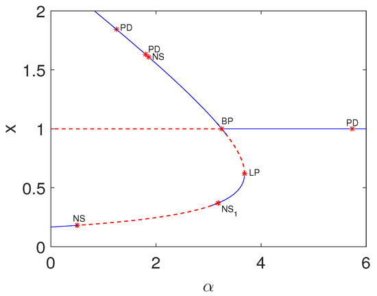
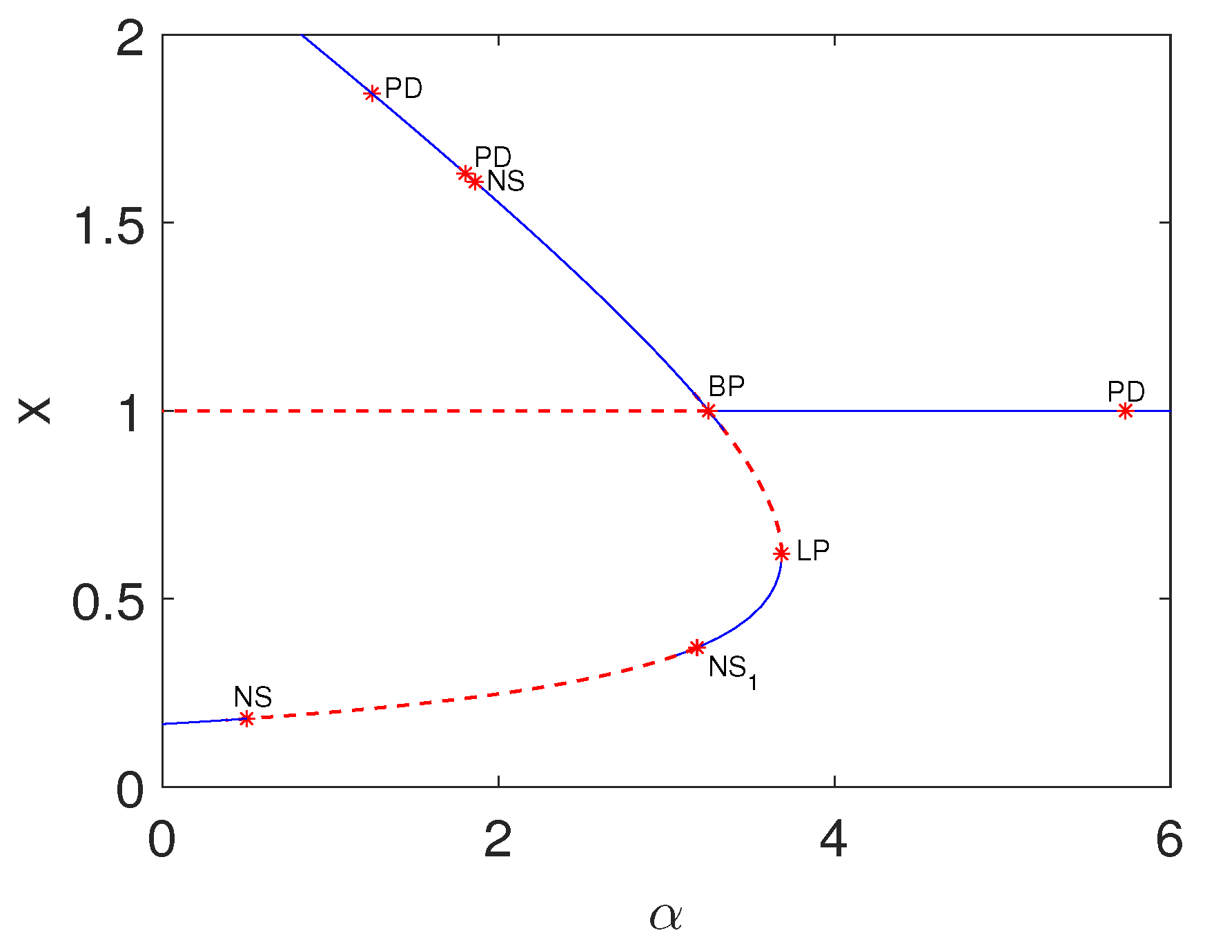
Fix $\gamma =1.3$, $m=2.5$, $\beta =0.5$, $\delta =1.04725$ and vary α in range $0<\alpha <6$. Then, we have ${\alpha }_0=m\gamma =3.25$, $\delta \ne 2$, and ${\alpha }_0\ne \beta {\gamma }^2=0.845$. The eigenvalues of $E_0$ are ${\lambda }_1=1$ and ${\lambda }_2=-0.04725$, satisfying $|{\lambda }_2|\ne 1$. From Theorem 4, map (3) will undergo a transcritical bifurcation at $E_0(1,0)$. The fixed point continuation curve diagram by using the continuation toolbox MatcontM [36,37] in the $(\alpha ,x)$ plane is given in Figure 1. The BP point in Figure 1 is the transcritical bifurcation point.

Figure 1. The fixed point continuation curve diagram in the $(\alpha ,x)$ plane. The blue solid line and the red dotted line indicate that the fixed points are stable and unstable, respectively. PD—period double point, NS—Neimark–Sacker bifurcation point, BP—branch point (transcritical bifurcation point), LP—limit point (fold bifurcation point). ${\mathrm{NS}}_1$ for $(x,y,\alpha ,\delta )$ is $(0.369896,0.630104,3.18133,1.04725)$. $\mathrm{LP}$ for $(x,y,\alpha ,\delta )$ is $(0.619139,0.380861,3.685165,1.04725)$.

3.2. Flip Bifurcation around $E_0(1,0)$

Next, we will present the flip bifurcation of the fixed point $E_0(1,0)$. To study the flip bifurcation, we must first consider the following Lemma 2 as stated in [38].

Lemma 2.

Let $f_{\mu }:\mathbb{R}\to \mathbb{R}$ be a one-parameter family of mappings such that $f_{{\mu }_0}$ has a fixed point $x_0$ with eigenvalue $-1$. Assume

(F1)

${\alpha }_1={\displaystyle \frac{\partial f}{\partial \mu }}·{\displaystyle \frac{{\partial }^{2}f}{\partial x^2}}+2{\displaystyle \frac{{\partial }^{2}f}{\partial x\partial \mu }}={\displaystyle \frac{\partial f}{\partial \mu }}·{\displaystyle \frac{{\partial }^{2}f}{\partial x^2}}-\left({\displaystyle \frac{\partial f}{\partial x}}-1\right){\displaystyle \frac{{\partial }^{2}f}{\partial x\partial \mu }}\ne 0$ at $\left(x_0,{\mu }_0\right)$;

(F2)

${\alpha }_2={\displaystyle \frac{1}{2}}{\left({\displaystyle \frac{{\partial }^{2}f}{\partial x^2}}\right)}^2+{\displaystyle \frac{1}{3}}\left({\displaystyle \frac{{\partial }^{3}f}{\partial x^3}}\right)\ne 0$ at $\left(x_0,{\mu }_0\right)$.

Then, there is a smooth curve of fixed points of $f_{\mu }$ passing through $\left(x_0,{\mu }_0\right)$, the stability of which changes at $\left(x_0,{\mu }_0\right)$. There is also a smooth curve γ passing through $\left(x_0,{\mu }_0\right)$ so that $\gamma -\left\{\left(x_0,{\mu }_0\right)\right\}$ is a union of hyperbolic period-2 orbits. The curve γ has quadratic tangency with the line $\mathbb{R}\times \left\{{\mu }_0\right\}$ at $\left(x_0,{\mu }_0\right)$.

In fact, based on Theorem 1 (IV)(ii) and (iii), we know that when $\alpha \ne m\gamma$, $\alpha \ne \gamma (1+m)$, if $\delta ={\displaystyle \frac{2\gamma }{\alpha -m\gamma }}$, or $\delta =2$, then one of the eigenvalues of $E_0$ is $-1$ and the magnitude of the other one is not 1. Here, we just consider the case $\delta ={\delta }_0\triangleq {\displaystyle \frac{2\gamma }{\alpha -m\gamma }}$, and the other case is very similar to this case so we omit it. The numerical simulation results are given later for Theorem 1 (IV)(iii). A perturbation system of system (3) is given as follows

$$\left\{\begin{array}{c}{x}_{n+1}=x_n+\left({\delta }_0+{\delta }^{*}\right)x_n\left(1-x_n-y_n\right),\hfill \\ y_{n+1}=y_n+\left({\delta }_0+{\delta }^{*}\right)y_n\left(m-{\displaystyle \frac{\beta y_n}{x_n}}-{\displaystyle \frac{\alpha }{\gamma +y_n}}\right),\hfill \end{array}\right.$$

(11)

where $|{\delta }^{*}|\ll 1$, which is a sufficient small perturbation parameter and is a new variable.

Letting $u_n=x_n-1$, $v_n=y_n$, we move the fixed point $E_0(1,0)$ to the origin $O(0,0)$. After that, we expand the right-hand side of map (11) with respect to the origin. Consequently, map (11) turns into

$$\left\{\begin{array}{c}\begin{array}{cc}\hfill u_{n+1}=& (1-{\delta }_0)u_n-{\delta }_0{v}_n-{\delta }_0{u}_n^2-{\delta }_0{u}_n{v}_n-u_n{\delta }^{*}-v_n{\delta }^{*}-u_n^2{\delta }^{*}-u_n{v}_n{\delta }^{*},\hfill \\ \hfill v_{n+1}=& -v_n-{\displaystyle \frac{\delta 0\left(\beta {\gamma }^2-\alpha \right)}{{\gamma }^2}}{v}_n^2+{\displaystyle \frac{m\gamma -\alpha }{\gamma }}{v}_n{\delta }^{*}+\beta {\delta }_0{u}_n{v}_n^2-{\displaystyle \frac{\beta {\gamma }^2-\alpha }{{\gamma }^2}}{v}_n^2{\delta }^{*}-{\displaystyle \frac{\alpha {\delta }_0}{{\gamma }^3}}{v}_n^3\hfill \\ \hfill & +\mathcal{O}\left(\parallel \left(u_n,v_n,{\delta }^{*}\right){\parallel }^4\right).\hfill \end{array}\hfill \end{array}\right.$$

(12)

Letting

$$T=\left(\begin{array}{cc}-{\delta }_0& -{\delta }_0\\ {\delta }_0-2& 0\end{array}\right)$$

and using the transformation

$$\left(\begin{array}{c}{u}_n\\ v_n\end{array}\right)=T\left(\begin{array}{c}{\phi }_n\\ {\psi }_n\end{array}\right),$$

then map (12) becomes

$$\left(\begin{array}{c}{\phi }_{n+1}\\ {\psi }_{n+1}\end{array}\right)=\left(\begin{array}{cc}-1& 0\\ 0& 1-{\delta }_0\end{array}\right)\left(\begin{array}{c}{\phi }_n\\ {\psi }_n\end{array}\right)+\left(\begin{array}{c}f\left({\phi }_n,{\psi }_n,{\delta }^{*}\right)\\ g\left({\phi }_n,{\psi }_n,{\delta }^{*}\right)\end{array}\right),$$

(13)

and, using the fact that ${\delta }_0={\displaystyle \frac{2\gamma }{\alpha -m\gamma }}$, we have

$$\begin{array}{cc}\hfill f\left({\phi }_n,{\psi }_n,{\delta }^{*}\right)=& -{\displaystyle \frac{4\left(m\gamma -\alpha +\gamma \right)\left(\beta {\gamma }^2-\alpha \right)}{\gamma {\left(m\gamma -\alpha \right)}^2}}{\phi }_n^2+{\displaystyle \frac{m\gamma -\alpha }{\gamma }}{\phi }_n{\delta }^{*}+{\displaystyle \frac{8\left(m\gamma -\alpha +\gamma \right)\left(\beta {\gamma }^4+m\alpha \gamma -{\alpha }^2+\alpha \gamma \right)}{{\gamma }^2{\left(m\gamma -\alpha \right)}^3}}{\phi }_n^3\hfill \\ \hfill & +{\displaystyle \frac{8\beta {\gamma }^2\left(m\gamma -\alpha +\gamma \right)}{{\left(m\gamma -\alpha \right)}^3}}{\phi }_n^2{\psi }_n+{\displaystyle \frac{2\left(\beta {\gamma }^2-\alpha \right)\left(m\gamma -\alpha +\gamma \right)}{{\gamma }^2\left(m\gamma -\alpha \right)}}{\phi }_n^2{\delta }^{*}+\mathcal{O}\left(\parallel \left({\phi }_n,{\psi }_n,{\delta }^{*}\right){\parallel }^4\right),\hfill \\ \hfill g\left({\phi }_n,{\psi }_n,{\delta }^{*}\right)=& {\displaystyle \frac{4\left[\left(\beta m+\beta -m\right){\gamma }^3+(1-\beta )\alpha {\gamma }^2-(m+1)\alpha \gamma +{\alpha }^2\right]}{\gamma {\left(m\gamma -\alpha \right)}^2}}{\phi }_n^2-{\displaystyle \frac{4\gamma \left(m\gamma -\alpha -\gamma \right)}{{\left(m\gamma -\alpha \right)}^2}}{\phi }_n{\psi }_n+{\displaystyle \frac{4{\gamma }^2}{{\left(m\gamma -\alpha \right)}^2}}{\psi }_n^2\hfill \\ \hfill & -{\psi }_n{\delta }^{*}-{\displaystyle \frac{8\left(m\gamma -\alpha +\gamma \right)\left(\beta {\gamma }^4+m\alpha \gamma -{\alpha }^2+\alpha \gamma \right)}{{\gamma }^2{\left(m\gamma -\alpha \right)}^3}}{\phi }_n^3-{\displaystyle \frac{8\beta {\gamma }^2\left(m\gamma -\alpha +\gamma \right)}{{\left(m\gamma -\alpha \right)}^3}}{\phi }_n^2{\psi }_n\hfill \\ \hfill & -{\displaystyle \frac{2\left[(\beta m+\beta -m){\gamma }^3+(1-\beta )\alpha {\gamma }^2-(m+1)\alpha \gamma +{\alpha }^2\right]}{{\gamma }^2\left(m\gamma -\alpha \right)}}{\phi }_n^2{\delta }^{*}-{\displaystyle \frac{2\gamma }{m\gamma -\alpha }}{\psi }_n^2{\delta }^{*}\hfill \\ \hfill & +{\displaystyle \frac{2\left(m\gamma -\alpha -\gamma \right)}{m\gamma -\alpha }}{\phi }_n{\psi }_n{\delta }^{*}+\mathcal{O}\left(\parallel \left({\phi }_n,{\psi }_n,{\delta }^{*}\right){\parallel }^4\right).\hfill \end{array}$$

According to the center manifold theory, the stability of $({\phi }_n,{\psi }_n)=(0,0)$ in the vicinity of ${\delta }^{*}=0$ can be determined by studying the following equations:

$$\begin{array}{c}{W}_{\mathrm{loc}}^c=\left\{\left({\phi }_n,{\psi }_n,{\delta }^{*}\right)\in {\mathbb{R}}^3|{\psi }_n=W_2({\phi }_n,{\delta }^{*})=b_1{\phi }_n^2+b_2{\phi }_n{\delta }^{*}+b_3{\delta }^{*2}+\mathcal{O}\left(\parallel \left({\phi }_n,{\delta }^{*}\right){\parallel }^3\right)\right\}.\hfill \end{array}$$

Just like in the previous subsection, we do not need to calculate $W_{\mathrm{loc}}^c$. The map, when restricted to the center manifold up to the third order, is presented as follows:

$$\begin{array}{c}{\phi }_{n+1}={\mathcal{F}}_2({\phi }_n,{\delta }^{*})=-{\phi }_n-{\displaystyle \frac{4\left(m\gamma -\alpha +\gamma \right)\left(\beta {\gamma }^2-\alpha \right)}{\gamma {\left(m\gamma -\alpha \right)}^2}}{\phi }_n^2+{\displaystyle \frac{m\gamma -\alpha }{\gamma }}{\phi }_n{\delta }^{*}+{\displaystyle \frac{2\left(\beta {\gamma }^2-\alpha \right)\left(m\gamma -\alpha +\gamma \right)}{{\gamma }^2\left(m\gamma -\alpha \right)}}{\phi }_n^2{\delta }^{*}\hfill \\ +{\displaystyle \frac{8\left(m\gamma -\alpha +\gamma \right)\left(\beta {\gamma }^4+m\alpha \gamma -{\alpha }^2+\alpha \gamma \right)}{{\gamma }^2{\left(m\gamma -\alpha \right)}^3}}{\phi }_n^3+\mathcal{O}\left(\parallel \left({\phi }_n,{\delta }^{*}\right){\parallel }^4\right).\hfill \end{array}$$

An easy calculation gives

$$\begin{array}{c}{\alpha }_1=\left({\displaystyle \frac{\partial {\mathcal{F}}_2}{\partial {\delta }^{*}}}·{\displaystyle \frac{{\partial }^2{\mathcal{F}}_2}{\partial {\phi }_n^2}}+2{\displaystyle \frac{{\partial }^2{\mathcal{F}}_2}{\partial {\phi }_n\partial {\delta }^{*}}}\right){|}_{(0,0)}={\displaystyle \frac{2\left(m\gamma -\alpha \right)}{\gamma }},\hfill \\ {\alpha }_2=\left[{\displaystyle \frac{1}{2}}{\left({\displaystyle \frac{{\partial }^2{\mathcal{F}}_2}{\partial {\phi }_n^2}}\right)}^2+{\displaystyle \frac{1}{3}}\left({\displaystyle \frac{{\partial }^3{\mathcal{F}}_2}{\partial {\phi }_n^3}}\right)\right]{|}_{(0,0)}={\displaystyle \frac{32{\left(m\gamma -\alpha +\gamma \right)}^2{\left(\beta {\gamma }^2-\alpha \right)}^2}{{\gamma }^2{\left(m\gamma -\alpha \right)}^4}}+{\displaystyle \frac{16\left(m\gamma -\alpha +\gamma \right)\left(\beta {\gamma }^4+m\alpha \gamma -{\alpha }^2+\alpha \gamma \right)}{{\gamma }^2{\left(m\gamma -\alpha \right)}^3}}.\hfill \end{array}$$

Theorem 5.

Map (3) undergoes a flip bifurcation at $E_0(1,0)$ if the following conditions are satisfied: $\delta ={\delta }_0\triangleq {\displaystyle \frac{2\gamma }{\alpha -m\gamma }}$, $\alpha \ne m\gamma$, $\alpha \ne \gamma (m+1)$, and ${\alpha }_1\ne 0$, ${\alpha }_2\ne 0$. Moreover, if ${\alpha }_2>0$ (resp., ${\alpha }_2<0$), the flip bifurcation is supercritical (or subcritical). That is to say, a period-2 orbit of map (3) emerges and it is stable (or unstable).

Example 2.

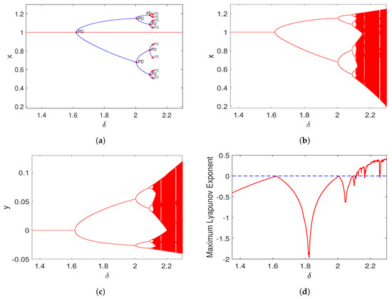
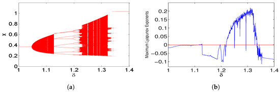
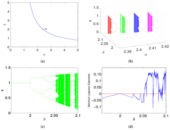
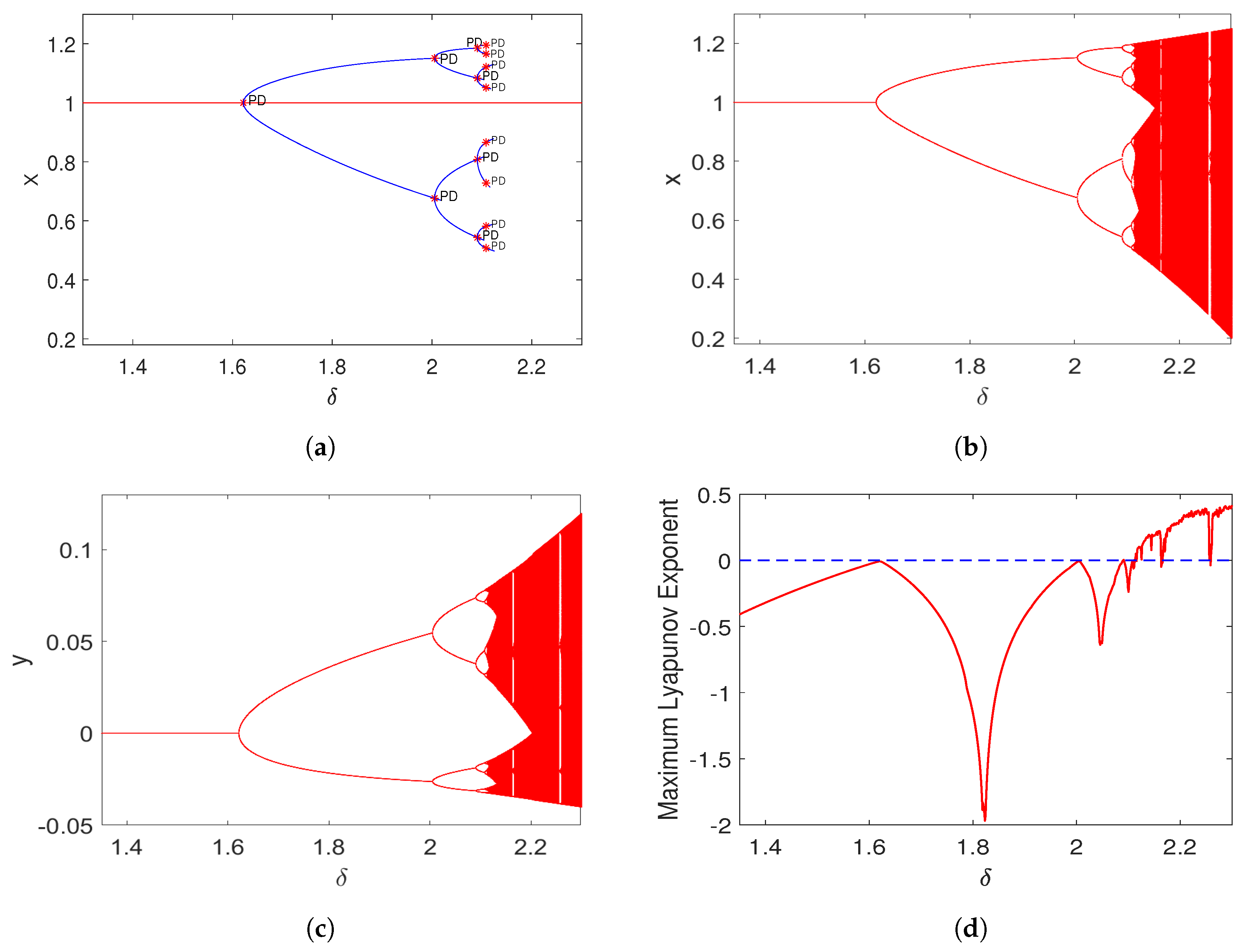
For the fixed point $E_0(1,0)$, if fix $\gamma =0.3$, $m=2.1$, $\alpha =1$, $\beta =0.4$, then we have ${\lambda }_1=-1$, ${\lambda }_2=-0.62162$, satisfying $|{\lambda }_2|\ne 1$ and ${\delta }_0={\displaystyle \frac{2\gamma }{\alpha -m\gamma }}=1.62162$, $\alpha =1\ne m\gamma =0.63$, $\alpha =1\ne \gamma (m+1)=0.93$, ${\alpha }_1=-2.46667\ne 0$, ${\alpha }_2=69.98585>0$. Based on Theorem 1 (I), when $0<\delta <{\delta }_0=1.62162<2$, then $0<\delta (\alpha -m\gamma )<2\gamma$ holds. Hence, the fixed point $E_0(1,0)$ is a sink, which is stable when $0<\delta <{\delta }_0$. Furthermore, according to Theorem 5, map (3) undergoes a supercritical flip bifurcation at $E_0(1,0)$ when δ crosses through the critical value ${\delta }_0$. That is, when $\delta >{\delta }_0$, $E_0(1,0)$ becomes unstable and a period-2 orbit appears. The cascade of period-doublings and bifurcation diagrams of map (3) for $1.35⩽\delta ⩽2.3$ with initial value $(x_0,y_0)=(0.01,0.01)$ are shown in Figure 2a–c, respectively. The corresponding maximum Lyapunov exponent is computed and presented in Figure 2d, which indicates the existence of chaotic sets when $\delta ⩾2.1$.

Figure 2. (a) A cascade of PD-points is visualized within the $(\delta ,x)$ plane for $\delta$ ranging from 1.35 to 2.3. The red line represents the continuation curve of the fixed point of the first iteration, and the blue line indicates the iteration number doubling when a new fixed-point curve emerges from a PD-point from left to right. The PD on the red line is at $(x,y,\delta )=(1,0,1.62162)$. (b) A bifurcation diagram in the $(\delta ,x)$ plane. (c) A bifurcation diagram in the $(\delta ,y)$ plane. (d) The maximum Lyapunov exponent corresponding to (a,b). Here, we have $\gamma =0.3$, $m=2.1$, $\alpha =1$, $\beta =0.4$ with an initial value of $(0.01,0.01)$, and the bifurcation value is $\delta =1.62162$.

Remark 1.

Recall that the meaning of x and y needs $x⩾0$ and $y⩾0$. We notice that in Figure 2c, the y value of lower branch of the bifurcation is less than zero. Although the bifurcation results calculated by the theoretical analysis are in accordance with Theorem 5, the diagram is merely in the mathematical rather than biological sense. Hence, from the biological point of view, the state variables satisfy $x⩾0$, $y⩾0$, which we will be focusing on.

Remark 2.

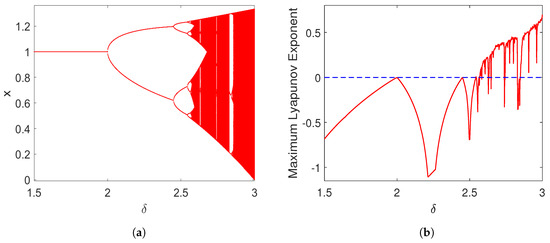
From Theorem 1 (IV)(iii), we know that if $\delta =2$, the fixed point $E_0(1,0)$ is also non-hyperbolic. Here we give a numerical simulation result for flip bifurcation when the bifurcation value $\delta =2$, $\alpha \ne m\gamma$ and $\alpha \ne \gamma (1+m)$. Fix $\gamma =0.2$, $m=0.8$, $\alpha =0.28$, $\beta =0.4$, $\delta =2$, then we have ${\lambda }_1=-1$, ${\lambda }_2=-0.2$, satisfying $|{\lambda }_2|\ne 1$ and $\alpha \ne m\gamma =0.16$, $\alpha \ne \gamma (1+m)=0.36$. The flip bifurcation diagram of map (3) in the $(\delta ,x)$ plane for $1.5⩽\delta ⩽3$ is illustrated in Figure 3a with the initial value $(x_0,y_0)=(0.01,0.01)$. The corresponding maximum Lyapunov exponent is calculated and presented in Figure 3b, which implies that there exists chaotic sets when $\delta ⩾2.6$.

Figure 3. (a) Bifurcation diagram in the $(\delta ,x)$ plane. (b) The maximum Lyapunov exponent corresponding to (a). Here $\gamma =0.2$, $m=0.8$, $\alpha =0.28$, $\beta =0.4$ with the initial value $(0.01,0.01)$. The bifurcation value is $\delta =2$.

3.3. Fold Bifurcation around $E_1$

For $E_1(x_1,y_1)$, if $\alpha ={\alpha }_1=\beta \gamma +2\beta +m\gamma +m-2\sqrt{\beta (\beta +m)(\gamma +1)}$, then ${\zeta }_{21}=0$ and ${\zeta }_{11}\ne 0$. The eigenvalues of $E_1$ are given by

$${\lambda }_1=1,{\lambda }_2={\zeta }_{11}\delta +1.$$

Suppose $\delta \ne -{\displaystyle \frac{2}{{\zeta }_{11}}}$, which leads $|{\lambda }_2|\ne 1$. Based on Theorem 3 (I), we know that $E_1$ may undergo a fold bifurcation. Choosing $\alpha$ as the bifurcation parameter, a perturbation system of system (3) is given as follows

$$\left\{\begin{array}{c}{x}_{n+1}=x_n+\delta x_n(1-x_n-y_n),\hfill \\ y_{n+1}=y_n+\delta y_n\left(m-{\displaystyle \frac{\beta y_n}{x_n}}-{\displaystyle \frac{{\alpha }_1+{\alpha }^{*}}{\gamma +y_n}}\right),\hfill \end{array}\right.$$

(14)

where $|{\alpha }^{*}|\ll 1$, which is a sufficiently small perturbation parameter and is a new variable.

Letting ${\xi }_n=x_n-x_1$, ${\eta }_n=y_n-y_1$, system (14) becomes

$$\left(\begin{array}{c}{\xi }_{n+1}\\ {\eta }_{n+1}\\ {\alpha }_{n+1}^{*}\end{array}\right)=\left(\begin{array}{ccc}{a}_{11}& a_{12}& 0\\ a_{21}& a_{22}& a_{23}\\ 0& 0& 1\end{array}\right)\left(\begin{array}{c}{\xi }_n\\ {\eta }_n\\ {\alpha }_n^{*}\end{array}\right)+\left(\begin{array}{c}F\left({\xi }_n,{\eta }_n,{\alpha }_n^{*}\right)\\ G\left({\xi }_n,{\eta }_n,{\alpha }_n^{*}\right)\\ 0\end{array}\right),$$

(15)

where

$$\begin{array}{c}{a}_{11}=1-\delta x_1,a_{12}=-\delta x_1,a_{21}={\displaystyle \frac{\beta \delta y_1^2}{x_1^2}},a_{22}=1+\delta m-{\displaystyle \frac{\delta \gamma {\alpha }_1}{{(\gamma +y_1)}^2}}-{\displaystyle \frac{2\beta \delta y_1}{x_1}},a_{23}=-{\displaystyle \frac{\delta y_1}{\gamma +y_1}},\hfill \\ F\left({\xi }_n,{\eta }_n,{\alpha }_n^{*}\right)=-\delta {\xi }_n^2-\delta {\xi }_n{\eta }_n,\hfill \\ G\left({\xi }_n,{\eta }_n,{\alpha }_n^{*}\right)=-{\displaystyle \frac{\beta \delta y_1^2}{x_1^3}}{\xi }_n^2+{\displaystyle \frac{2\beta \delta y_1}{x_1^2}}{\xi }_n{\eta }_n-{\displaystyle \frac{\delta \gamma }{{\left(\gamma +y_1\right)}^2}}{\eta }_n{\alpha }_n^{*}+\left({\displaystyle \frac{\delta \gamma {\alpha }_1}{{\left(\gamma +y_1\right)}^3}}-{\displaystyle \frac{\beta \delta }{x_1}}\right){\eta }_n^2+{\displaystyle \frac{\beta \delta y_1^2}{x_1^4}}{\xi }_n^3\hfill \\ -{\displaystyle \frac{2\beta \delta y_1}{x_1^3}}{\xi }_n^2{\eta }_n+{\displaystyle \frac{\beta \delta }{x_1^2}}{\xi }_n{\eta }_n^2-{\displaystyle \frac{\delta \gamma {\alpha }_1}{{\left(\gamma +y_1\right)}^4}}{\eta }_n^3+{\displaystyle \frac{\delta \gamma }{{\left(\gamma +y_1\right)}^3}}{\eta }_n^2{\alpha }_n^{*}+\mathcal{O}\left(\parallel \left({\xi }_n,{\eta }_n,{\alpha }_n^{*}\right){\parallel }^4\right).\hfill \end{array}$$

Letting

$$T=\left(\begin{array}{ccc}{\displaystyle \frac{a_{12}}{{\lambda }_2-a_{11}}}& 1& {\displaystyle \frac{a_{12}-1}{1-a_{11}}}\\ 1& {\displaystyle \frac{1-a_{11}}{a_{12}}}& 1\\ 0& 0& {\displaystyle \frac{-a_{12}{a}_{21}-{(a_{11}-1)}^2}{a_{12}{a}_{23}(a_{11}-1)}}\end{array}\right)$$

and using the following transformation

$$\left(\begin{array}{c}{\xi }_n\\ {\eta }_n\\ {\alpha }_n^{*}\end{array}\right)=T\left(\begin{array}{c}{\phi }_n\\ {\psi }_n\\ {\tilde{\alpha }}_n^{*}\end{array}\right),$$

map (15) is transformed as

$$\left(\begin{array}{c}{\phi }_{n+1}\\ {\psi }_{n+1}\\ {\tilde{\alpha }}_{n+1}^{*}\end{array}\right)=\left(\begin{array}{ccc}{\lambda }_2& 0& 0\\ 0& 1& 1\\ 0& 0& 1\end{array}\right)\left(\begin{array}{c}{\phi }_n\\ {\psi }_n\\ {\tilde{\alpha }}_n^{*}\end{array}\right)+\left(\begin{array}{c}f\left({\phi }_n,{\psi }_n,{\tilde{\alpha }}_n^{*}\right)\\ g\left({\phi }_n,{\psi }_n,{\tilde{\alpha }}_n^{*}\right)\\ 0\end{array}\right),$$

(16)

where

$$\begin{array}{cc}\hfill f\left({\phi }_n,{\psi }_n,{\tilde{\alpha }}_n^{*}\right)=& \left({\displaystyle \frac{\delta (a_{11}-{\lambda }_2)(a_{11}-1)}{a_{12}({\lambda }_2-1)}}+{\displaystyle \frac{\beta \delta y_1^2(a_{11}-{\lambda }_2)}{({\lambda }_2-1)x_1^3}}\right){\xi }_n^2+\left({\displaystyle \frac{\delta (a_{11}-{\lambda }_2)(a_{11}-1)}{a_{12}({\lambda }_2-1)}}-{\displaystyle \frac{2\beta \delta y_1(a_{11}-{\lambda }_2)}{({\lambda }_2-1)x_1^2}}\right){\xi }_n{\eta }_n\hfill \\ \hfill & +{\displaystyle \frac{{\lambda }_2-a_{11}}{{\lambda }_2-1}}\left({\displaystyle \frac{\delta \gamma {\alpha }_1}{{(\gamma +y_1)}^3}}-{\displaystyle \frac{\beta \delta }{x_1}}\right){\eta }_n^2+{\displaystyle \frac{\delta \gamma (a_{11}-{\lambda }_2)}{({\lambda }_2-1){(\gamma +y_1)}^2}}{\eta }_n{\alpha }_n^{*}-{\displaystyle \frac{\beta \delta y_1^2(a_{11}-{\lambda }_2)}{({\lambda }_2-1)x_1^4}}{\xi }_n^3\hfill \\ \hfill & +{\displaystyle \frac{2\beta \delta y_1(a_{11}-{\lambda }_2)}{({\lambda }_2-1)x_1^3}}{\xi }_n^2{\eta }_n-{\displaystyle \frac{\beta \delta (a_{11}-{\lambda }_2)}{({\lambda }_2-1)x_1^2}}{\xi }_n{\eta }_n^2+{\displaystyle \frac{\delta \gamma {\alpha }_1(a_{11}-{\lambda }_2)}{({\lambda }_2-1){(\gamma +y_1)}^4}}{\eta }_n^3\hfill \\ \hfill & -{\displaystyle \frac{\delta \gamma (a_{11}-{\lambda }_2)}{({\lambda }_2-1){(\gamma +y_1)}^3}}{\eta }_n^2{\alpha }_n^{*}+\mathcal{O}\left(\parallel \left({\xi }_n,{\eta }_n,{\alpha }_n^{*}\right){\parallel }^4\right),\hfill \\ \hfill g\left({\phi }_n,{\psi }_n,{\tilde{\alpha }}_{*}\right)=& \left({\displaystyle \frac{\delta (a_{11}-{\lambda }_2)}{{\lambda }_2-1}}+{\displaystyle \frac{a_{12}\beta \delta y_1^2}{({\lambda }_2-1)x_1^3}}\right){\xi }_n^2+\left({\displaystyle \frac{\delta (a_{11}-{\lambda }_2)}{{\lambda }_2-1}}-{\displaystyle \frac{2a_{12}\beta \delta y_1}{({\lambda }_2-1)x_1^2}}\right){\xi }_n{\eta }_n-{\displaystyle \frac{a_{12}}{{\lambda }_2-1}}\left({\displaystyle \frac{\delta \gamma {\alpha }_1}{{(\gamma +y_1)}^3}}-{\displaystyle \frac{\beta \delta }{x_1}}\right){\eta }_n^2\hfill \\ \hfill & +{\displaystyle \frac{a_{12}\delta \gamma }{{(\gamma +y_1)}^2({\lambda }_2-1)}}{\eta }_n{\alpha }_n^{*}-{\displaystyle \frac{a_{12}\beta \delta y_1^2}{({\lambda }_2-1)x_1^4}}{\xi }_n^3+{\displaystyle \frac{2a_{12}\beta \delta y_1}{({\lambda }_2-1)x_1^3}}{\xi }_n^2{\eta }_n-{\displaystyle \frac{a_{12}\beta \delta }{({\lambda }_2-1)x_1^2}}{\xi }_n{\eta }_n^2\hfill \\ \hfill & +{\displaystyle \frac{a_{12}\delta \gamma {\alpha }_1}{{(\gamma +y_1)}^4({\lambda }_2-1)}}{\eta }_n^3-{\displaystyle \frac{a_{12}\delta \gamma }{{(\gamma +y_1)}^3({\lambda }_2-1)}}{\eta }_n^2{\alpha }_n^{*}+\mathcal{O}\left(\parallel \left({\xi }_n,{\eta }_n,{\alpha }_n^{*}\right){\parallel }^4\right),\hfill \\ \hfill {\xi }_n={\displaystyle \frac{a_{12}}{{\lambda }_2-a_{11}}}{\phi }_n& +{\psi }_n+{\displaystyle \frac{a_{12}-1}{1-a_{11}}}{\tilde{\alpha }}_n^{*},{\eta }_n={\phi }_n+{\displaystyle \frac{1-a_{11}}{a_{12}}}{\psi }_n+{\tilde{\alpha }}_n^{*},{\alpha }_n^{*}={\displaystyle \frac{-a_{12}{a}_{21}-{(a_{11}-1)}^2}{a_{12}{a}_{23}(a_{11}-1)}}{\tilde{\alpha }}_n^{*}.\hfill \end{array}$$

Due to the center manifold depending on parameters theory, the stability of $({\phi }_n,{\psi }_n)=(0,0)$ near ${\alpha }^{*}=0$ can be determined by studying a one-parameter family of reduced equations on a center manifold, which can be represented as follows

$$\begin{array}{c}{W}_{\mathrm{loc}}^c=\left\{({\phi }_n,{\psi }_n,{\tilde{\alpha }}_n^{*})\in {\mathbb{R}}^3|{\phi }_n=W_3({\psi }_n,{\tilde{\alpha }}_n^{*})=c_1{\psi }_n^2+c_2{\psi }_n{\tilde{\alpha }}_n^{*}+c_3{\tilde{\alpha }}_n^{*2}+\mathcal{O}\left(\parallel \left({\psi }_n,{\tilde{\alpha }}_n^{*}\right){\parallel }^3\right)\right\}\hfill \end{array}$$

and from map (16), we have

$${\psi }_{n+1}={\psi }_n+{\tilde{\alpha }}_n^{*}+g\left({\phi }_n,{\psi }_n,{\tilde{\alpha }}_n^{*}\right)={\psi }_n+{\tilde{\alpha }}_n^{*}+g\left(W_3({\psi }_n,{\tilde{\alpha }}_n^{*}),{\psi }_n,{\tilde{\alpha }}_n^{*}\right),$$

from which it follows that

$$\begin{array}{cc}\hfill {\phi }_{n+1}& =W_3\left({\psi }_{n+1},{\tilde{\alpha }}_{n+1}^{*}\right)=W_3({\psi }_n+{\tilde{\alpha }}_n^{*}+g\left(W_3({\psi }_n,{\tilde{\alpha }}_n^{*}),{\psi }_n,{\tilde{\alpha }}_n^{*}\right),{\tilde{\alpha }}_n^{*})\hfill \\ \hfill & =c_1{\psi }_n^2+(2c_1+c_2){\psi }_n{\tilde{\alpha }}_n^{*}+(c_1+c_2+c_3){\tilde{\alpha }}_n^{*2}+\mathcal{O}\left(\parallel \left({\psi }_n,{\tilde{\alpha }}_n^{*}\right){\parallel }^3\right).\hfill \end{array}$$

(17)

On the other hand,

$$\begin{array}{cc}\hfill {\phi }_{n+1}& ={\lambda }_2{\phi }_n+f({\phi }_n,{\psi }_n,{\tilde{\alpha }}_n^{*})={\lambda }_2{W}_3({\psi }_n,{\tilde{\alpha }}_n^{*})+f\left(W_3({\psi }_n,{\tilde{\alpha }}_n^{*}),{\psi }_n,{\tilde{\alpha }}_n^{*}\right)\hfill \\ \hfill & =\left({\displaystyle \frac{{(1-a_{11})}^2{f}_{020}}{a_{12}^2}}+{\displaystyle \frac{(1-a_{11})f_{110}}{a_{12}}}+c_1{\lambda }_2+f_{200}\right){\psi }_n^2\hfill \\ \hfill & +\left({\displaystyle \frac{(a_{12}-1)f_{110}}{a_{12}}}-{\displaystyle \frac{(1-a_{11})(a_{12}{a}_{21}+{(a_{11}-1)}^2)f_{011}}{a_{12}^2{a}_{23}(a_{11}-1)}}+{\displaystyle \frac{2(a_{12}-1)f_{200}}{1-a_{11}}}+{\displaystyle \frac{2(1-a_{11})f_{020}}{a_{12}}}+c_2{\lambda }_2+f_{110}\right){\psi }_n{\tilde{\alpha }}_n^{*}\hfill \\ \hfill & +\left({\displaystyle \frac{{(a_{12}-1)}^2{f}_{200}}{{(1-a_{11})}^2}}+{\displaystyle \frac{(a_{12}-1)f_{110}}{1-a_{11}}}-{\displaystyle \frac{(a_{12}{a}_{21}+{(a_{11}-1)}^2)f_{011}}{a_{12}{a}_{23}(a_{11}-1)}}+c_3{\lambda }_2+f_{020}\right){\tilde{\alpha }}_n^{*2}+\mathcal{O}\left(\parallel ({\psi }_n,{\tilde{\alpha }}_n^{*}){\parallel }^3\right).\hfill \end{array}$$

(18)

where

$$\begin{array}{c}{f}_{200}={\displaystyle \frac{\delta (a_{11}-{\lambda }_2)(a_{11}-1)}{a_{12}({\lambda }_2-1)}}+{\displaystyle \frac{\beta \delta y_1^2(a_{11}-{\lambda }_2)}{({\lambda }_2-1)x_1^3}},f_{110}={\displaystyle \frac{\delta (a_{11}-{\lambda }_2)(a_{11}-1)}{a_{12}({\lambda }_2-1)}}-{\displaystyle \frac{2\beta \delta y_1(a_{11}-{\lambda }_2)}{({\lambda }_2-1)x_1^2}},\hfill \\ f_{020}={\displaystyle \frac{{\lambda }_2-a_{11}}{{\lambda }_2-1}}\left({\displaystyle \frac{\delta \gamma {\alpha }_1}{{(\gamma +y_1)}^3}}-{\displaystyle \frac{\beta \delta }{x_1}}\right),f_{011}={\displaystyle \frac{\delta \gamma (a_{11}-{\lambda }_2)}{({\lambda }_2-1){(\gamma +y_1)}^2}}.\hfill \end{array}$$

Comparing the coefficients of like power in (18) with those in (17) gives

$$\begin{array}{c}{c}_1=-{\displaystyle \frac{{(a_{11}-1)}^2{f}_{020}}{a_{12}^2({\lambda }_2-1)}}+{\displaystyle \frac{(a_{11}-1)f_{110}}{a_{12}({\lambda }_2-1)}}-{\displaystyle \frac{f_{200}}{{\lambda }_2-1}},\hfill \\ c_2=-{\displaystyle \frac{{(a_{11}-1)}^2{f}_{011}}{a_{12}^2{a}_{23}({\lambda }_2-1)}}-{\displaystyle \frac{a_{21}{f}_{011}}{a_{12}{a}_{23}({\lambda }_2-1)}}+{\displaystyle \frac{2(a_{11}-1)f_{020}+f_{110}}{a_{12}({\lambda }_2-1)}}+{\displaystyle \frac{2(c_1-f_{110})}{{\lambda }_2-1}}+{\displaystyle \frac{2f_{200}(a_{12}-1)}{(a_{11}-1)({\lambda }_2-1)}},\hfill \\ c_3={\displaystyle \frac{(a_{11}-1)f_{011}}{a_{12}{a}_{23}({\lambda }_2-1)}}+{\displaystyle \frac{a_{21}{f}_{011}}{a_{23}({\lambda }_2-1)(a_{11}-1)}}-{\displaystyle \frac{{(a_{12}-1)}^2{f}_{200}}{{(a_{11}-1)}^2({\lambda }_2-1)}}+{\displaystyle \frac{(a_{12}-1)f_{110}}{({\lambda }_2-1)(a_{11}-1)}}+{\displaystyle \frac{c_1+c_2-f_{020}}{{\lambda }_2-1}}.\hfill \end{array}$$

Therefore, the map, which is restricted to the center manifold is presented as follows:

$$\begin{array}{c}{\psi }_{n+1}={\mathcal{F}}_3({\psi }_n,{\tilde{\alpha }}_n^{*})={\psi }_n+{\tilde{\alpha }}_n^{*}+k_1{\psi }_n^2+k_2{\psi }_n{\tilde{\alpha }}_n^{*}+k_3{\tilde{\alpha }}_n^{*2},\hfill \end{array}$$

where

$$\begin{array}{cc}\hfill k_1=& {\displaystyle \frac{{(a_{11}-1)}^2{g}_{020}}{a_{12}^2}}-{\displaystyle \frac{(a_{11}-1)g_{110}}{a_{12}}}+g_{200},\hfill \\ \hfill k_2=& {\displaystyle \frac{{(a_{11}-1)}^2{g}_{011}}{a_{12}^2{a}_{23}}}+{\displaystyle \frac{a_{21}{g}_{011}}{a_{12}{a}_{23}}}+{\displaystyle \frac{2(1-a_{11})g_{020}-g_{110}}{a_{12}}}-{\displaystyle \frac{2(a_{12}-1)g_{200}}{a_{11}-1}}+2g_{110},\hfill \\ \hfill k_3=& -{\displaystyle \frac{(a_{11}-1)g_{011}}{a_{12}{a}_{23}}}-{\displaystyle \frac{a_{21}{g}_{011}}{(a_{11}-1)a_{23}}}-{\displaystyle \frac{(a_{12}-1)g_{110}}{a_{11}-1}}+{\displaystyle \frac{{(a_{12}-1)}^2{g}_{200}}{{(a_{11}-1)}^2}}+g_{020},\hfill \end{array}$$

and

$$\begin{array}{c}{g}_{200}={\displaystyle \frac{\delta (a_{11}-{\lambda }_2)}{{\lambda }_2-1}}+{\displaystyle \frac{a_{12}\beta \delta y_1^2}{({\lambda }_2-1)x_1^3}},g_{110}={\displaystyle \frac{\delta (a_{11}-{\lambda }_2)}{{\lambda }_2-1}}-{\displaystyle \frac{2a_{12}\beta \delta y_1}{({\lambda }_2-1)x_1^2}},\hfill \\ g_{020}=-{\displaystyle \frac{a_{12}}{{\lambda }_2-1}}\left({\displaystyle \frac{\delta \gamma {\alpha }_1}{{(\gamma +y_1)}^3}}-{\displaystyle \frac{\beta \delta }{x_1}}\right),g_{011}={\displaystyle \frac{a_{12}\delta \gamma }{{(\gamma +y_1)}^2({\lambda }_2-1)}}.\hfill \end{array}$$

We have

$$\begin{array}{c}{\mathcal{F}}_3(0,0)=0,{\displaystyle \frac{\partial {\mathcal{F}}_3}{\partial {\psi }_n}}(0,0)=1,{\displaystyle \frac{\partial {\mathcal{F}}_3}{\partial {\tilde{\alpha }}_n^{*}}}(0,0)=1,\hfill \\ {\displaystyle \frac{{\partial }^2{\mathcal{F}}_3}{\partial {\psi }_n^2}}(0,0)=2\left({\displaystyle \frac{{(a_{11}-1)}^2{g}_{020}}{a_{12}^2}}-{\displaystyle \frac{(a_{11}-1)g_{110}}{a_{12}}}+g_{200}\right).\hfill \end{array}$$

Hence, if ${\displaystyle \frac{{(a_{11}-1)}^2{g}_{020}}{a_{12}^2}}-{\displaystyle \frac{(a_{11}-1)g_{110}}{a_{12}}}+g_{200}\ne 0$, then a fold bifurcation occurs at $E_1$.

Theorem 6.

If the quadratic normal form coefficient ${\displaystyle \frac{{(a_{11}-1)}^2{g}_{020}}{a_{12}^2}}-{\displaystyle \frac{(a_{11}-1)g_{110}}{a_{12}}}+g_{200}\ne 0$ and the conditions ${\zeta }_{21}=0$ and ${\zeta }_{11}\ne 0$ hold, then system (3) undergoes a fold bifurcation at $E_1$. Moreover, if ${\displaystyle \frac{{(a_{11}-1)}^2{g}_{020}}{a_{12}^2}}-{\displaystyle \frac{(a_{11}-1)g_{110}}{a_{12}}}+g_{200}>0(<0)$, then two fixed points bifurcate from $E_1$ for $\alpha <{\alpha }_1(\alpha >{\alpha }_1)$, coalesce as α increases (decreases) through ${\alpha }_1$ and then disappear when $\alpha >{\alpha }_1(\alpha <{\alpha }_1)$.

Example 3.

Fix $\gamma =1.3$, $m=2.5$, $\beta =0.5$, $\delta =1.04725$. We have $E_1(0.619139,0.380861)$, ${\alpha }_1=\beta \gamma +2\beta +m\gamma +m-2\sqrt{\beta (\beta +m)(\gamma +1)}=3.685157$, ${\zeta }_{21}=0$ and ${\zeta }_{11}=-0.429936991$. The eigenvalues of $E_1$ are ${\lambda }_1=1$ and ${\lambda }_2=0.549749$, satisfying $|{\lambda }_2|\ne 1$. Furthermore, we have $a_{11}=0.351607$, $a_{12}=-0.648393$, $a_{21}=0.198142$, $a_{22}=1.198141$, $g_{200}=0.921729$, $g_{110}=-1.037524$, $g_{020}=-0.303473$, $g_{011}=0.693927$, ${\displaystyle \frac{{(a_{11}-1)}^2{g}_{020}}{a_{12}^2}}-{\displaystyle \frac{(a_{11}-1)g_{110}}{a_{12}}}+g_{200}=1.655780<0$. From Theorem 6, map (3) will undergo a fold bifurcation at $E_1(0.619139,0.380861)$ and two fixed points bifurcate from $E_1$ for $\alpha <{\alpha }_1=3.685157$, coalesce as α increase through ${\alpha }_1$, and then disappear when $\alpha >{\alpha }_1=3.685157$. The fixed point continuation curve diagram by using the continuation toolbox MatcontM [36,37] in the $(\alpha ,x)$ plane is given in Figure 1. The LP point in Figure 1 is the fold bifurcation point.

3.4. Flip Bifurcation around the Positive Fixed Points $E_k$

Next, we consider the flip bifurcation of the positive fixed point $E_k\left(x_k,y_k\right)$$(k=1,2,3)$. From Theorem 3 (II), if $\delta ={\delta }_{1k}={\displaystyle \frac{-{\zeta }_{1k}-\sqrt{\Delta }}{{\zeta }_{2k}}}$ or $\delta ={\delta }_{2k}={\displaystyle \frac{-{\zeta }_{1k}+\sqrt{\Delta }}{{\zeta }_{2k}}}$, then $E_k(x_k,y_k)$$(k=1,2,3)$ is a non-hyperbolic fixed point. Let $E_{*}(x_{*},y_{*})$ be denoted one of the positive fixed points, ${\delta }_i\triangleq {\delta }_{ik}$ and ${\zeta }_i\triangleq {\zeta }_{ik}$$(i=1,2)$ for simplicity. Here, we only take the flip bifurcation into account when $\delta$ changes within a small neighborhood of ${\delta }_1$. Similar statements hold for the neighborhood of ${\delta }_2$. If $\delta ={\delta }_1$, the eigenvalues of the Jacobian of $E_{*}(x_{*},y_{*})$ are given by

$${\lambda }_1=-1,{\lambda }_2=-{\zeta }_2{\delta }_1^2-{\zeta }_1{\delta }_1-1.$$

If ${\zeta }_1{\delta }_1\ne -2,-4$, then $|{\lambda }_2|\ne 1$. A perturbation system of system (3) can be written as

$$\left\{\begin{array}{c}{x}_{n+1}=x_n+\left({\delta }_1+{\delta }_{*}\right)x_n\left(1-x_n-y_n\right),\hfill \\ y_{n+1}=y_n+\left({\delta }_1+{\delta }_{*}\right)y_n\left(m-{\displaystyle \frac{\beta y_n}{x_n}}-{\displaystyle \frac{\alpha }{\gamma +y_n}}\right),\hfill \end{array}\right.$$

(19)

where $|{\delta }_{*}|\ll 1$ and it acts as a small perturbation parameter.

We let $u_n=x_n-x_{*}$ and $v_n=y_n-y_{*}$ to transform the fixed point $(x_{*},y_{*})$ to $O(0,0)$. Map (19) becomes

$$\left\{\begin{array}{cc}{u}_{n+1}\hfill & =a_{11}{u}_n+a_{12}{v}_n+a_{200}{u}_n^2+a_{110}{u}_n{v}_n+a_{101}{u}_n{\delta }_{*}+a_{011}{v}_n{\delta }_{*}+a_{201}{u}_n^2{\delta }_{*}+a_{111}{u}_n{v}_n{\delta }_{*},\hfill \\ v_{n+1}\hfill & =a_{21}{u}_n+a_{22}{v}_n+b_{200}{u}_n^2+b_{110}{u}_n{v}_n+b_{020}{v}_n^2+b_{101}{u}_n{\delta }_{*}+b_{011}{v}_n{\delta }_{*}+b_{111}{u}_n{v}_n{\delta }_{*}+b_{300}{u}_n^3\hfill \\ \hfill & +b_{210}{u}_n^2{v}_n+b_{120}{u}_n{v}_n^2+b_{201}{u}_n^2{\delta }_{*}+b_{021}{v}_n^2{\delta }_{*}+b_{030}{v}_n^3+\mathcal{O}\left(\parallel (u_n,v_n,{\delta }_{*}){\parallel }^4\right),\hfill \end{array}\right.$$

(20)

where

$$\begin{array}{c}{a}_{11}=1-{\delta }_1{x}_{*},a_{12}=-{\delta }_1{x}_{*},a_{200}=-{\delta }_1,a_{110}=-{\delta }_1,a_{101}=-x_{*},a_{011}=-x_{*},\hfill \\ a_{201}=-1,a_{111}=-1,a_{21}=\beta {\delta }_1{\left({\displaystyle \frac{y_{*}}{x_{*}}}\right)}^2,a_{22}=1+m{\delta }_1-{\displaystyle \frac{2\beta {\delta }_1{y}_{*}}{x_{*}}}-{\displaystyle \frac{\alpha {\delta }_1\gamma }{{(\gamma +y_{*})}^2}},\hfill \\ b_{200}=-{\displaystyle \frac{\beta {\delta }_1{y}_{*}^2}{x_{*}^3}},b_{110}={\displaystyle \frac{2\beta {\delta }_1{y}_{*}}{x_{*}^2}},b_{020}={\displaystyle \frac{\alpha {\delta }_1\gamma }{{(\gamma +y_{*})}^3}}-{\displaystyle \frac{\beta {\delta }_1}{x_{*}}},b_{101}=\beta {\left({\displaystyle \frac{y_{*}}{x_{*}}}\right)}^2,\hfill \\ b_{011}=m-{\displaystyle \frac{2\beta y_{*}}{x_{*}}}-{\displaystyle \frac{\alpha \gamma }{{\left(\gamma +y_{*}\right)}^2}},b_{111}={\displaystyle \frac{2\beta y_{*}}{x_{*}^2}},b_{300}={\displaystyle \frac{\beta {\delta }_1{y}_{*}^2}{x_{*}^4}},b_{210}=-{\displaystyle \frac{2\beta {\delta }_1{y}_{*}}{x_{*}^3}},\hfill \\ b_{120}={\displaystyle \frac{\beta {\delta }_1}{x_{*}^2}},b_{201}=-{\displaystyle \frac{\beta y_{*}^2}{x_{*}^3}},b_{021}={\displaystyle \frac{\alpha \gamma }{{(\gamma +y_{*})}^3}}-{\displaystyle \frac{\beta }{x_{*}}},b_{030}=-{\displaystyle \frac{\alpha {\delta }_1\gamma }{{(\gamma +y_{*})}^4}}.\hfill \end{array}$$

Since $a_{12}=-{\delta }_1{x}_{*}\ne 0$, we can construct an invertible matrix as follows

$$T=\left(\begin{array}{cc}1& -1\\ {\displaystyle \frac{a_{22}-{\lambda }_2}{a_{12}}}& -{\displaystyle \frac{a_{22}+1}{a_{12}}}\end{array}\right),$$

and use the transform

$$\left(\begin{array}{c}{u}_n\\ v_n\end{array}\right)=T\left(\begin{array}{c}{\phi }_n\\ {\psi }_n\end{array}\right),$$

then map (20) becomes

$$\left(\begin{array}{c}{\phi }_{n+1}\\ {\psi }_{n+1}\end{array}\right)=\left(\begin{array}{cc}-1& 0\\ 0& {\lambda }_2\end{array}\right)\left(\begin{array}{c}{\phi }_n\\ {\psi }_n\end{array}\right)+\left(\begin{array}{c}f({\phi }_n,{\psi }_n,{\delta }_{*})\\ g({\phi }_n,{\psi }_n,{\delta }_{*})\end{array}\right),$$

(21)

where

$$\begin{array}{cc}f\left({\phi }_n,{\psi }_n,{\delta }_{*}\right)\hfill & =p_{200}{\phi }_n^2+p_{110}{\phi }_n{\psi }_n+p_{020}{\psi }_n^2+p_{101}{\phi }_n{\delta }_{*}+p_{011}{\psi }_n{\delta }_{*}+p_{300}{\phi }_n^3\hfill \\ \hfill & +p_{210}{\phi }_n^2{\psi }_n+p_{120}{\phi }_n{\psi }_n^2+p_{030}{\psi }_n^3+p_{201}{\phi }_n^2{\delta }_{*}+p_{021}{\psi }_n^2{\delta }_{*}+p_{111}{\phi }_n{\psi }_n{\delta }_{*}\hfill \\ \hfill & +\mathcal{O}\left(\parallel ({\phi }_n,{\psi }_n,{\delta }_{*}){\parallel }^4\right),\hfill \\ g\left({\phi }_n,{\psi }_n,{\delta }_{*}\right)\hfill & =q_{200}{\phi }_n^2+q_{110}{\phi }_n{\psi }_n+q_{020}{\psi }_n^2+q_{101}{\phi }_n{\delta }_{*}+q_{011}{\psi }_n{\delta }_{*}+q_{300}{\phi }_n^3\hfill \\ \hfill & +q_{210}{\phi }_n^2{\psi }_n+q_{120}{\phi }_n{\psi }_n^2+q_{030}{\psi }_n^3+q_{201}{\phi }_n^2{\delta }_{*}+q_{021}{\psi }_n^2{\delta }_{*}+q_{111}{\phi }_n{\psi }_n{\delta }_{*}\hfill \\ \hfill & +\mathcal{O}\left(\parallel ({\phi }_n,{\psi }_n,{\delta }_{*}){\parallel }^4\right),\hfill \end{array}$$

(22)

and the coefficients of $f\left({\phi }_n,{\psi }_n,{\delta }_{*}\right)$ and $g\left({\phi }_n,{\psi }_n,{\delta }_{*}\right)$ are given in Appendix D.

According to the center manifold theory, we know that there is a center manifold that can be approximately expressed as follows

$$\begin{array}{c}{W}_{\mathrm{loc}}^c(0,0)=\left\{\left({\phi }_n,{\psi }_n,{\delta }_{*}\right)\in {\mathbb{R}}^3|{\psi }_n=W_4({\phi }_n,{\delta }_{*})=d_1{\phi }_n^2+d_2{\phi }_n{\delta }_{*}+d_3{\delta }_{*}^2+\mathcal{O}\left(\parallel ({\phi }_n,{\delta }_{*}){\parallel }^3\right)\right\},\hfill \end{array}$$

where $\mathcal{O}\left(\parallel (u_n,{\delta }_{*}){\parallel }^3\right)$ represents a function whose order with respect to its variables is at least 3. Recall from map (21) that we have

$${\phi }_{n+1}=-{\phi }_n+f\left({\phi }_n,{\psi }_n,{\delta }_{*}\right)=-{\phi }_n+f\left({\phi }_n,W_4({\phi }_n,{\delta }_{*}),{\delta }_{*}\right),$$

from which it follows that

$$\begin{array}{cc}\hfill {\psi }_{n+1}& =W_4({\phi }_{n+1},{\delta }_{*})=W_4\left(-{\phi }_n+f\left({\phi }_n,W_4({\phi }_n,{\delta }_{*}),{\delta }_{*}\right),{\delta }_{*}\right)\hfill \\ \hfill & =d_1{\phi }_n^2-d_2{\phi }_n{\delta }_{*}+d_3{\delta }_{*}^2+\mathcal{O}\left(\parallel ({\phi }_n,{\delta }_{*}){\parallel }^3\right).\hfill \end{array}$$

(23)

On the other hand,

$$\begin{array}{cc}\hfill {\psi }_{n+1}& ={\lambda }_2{\psi }_n+g\left({\phi }_n,{\psi }_n,{\delta }_{*}\right)={\lambda }_2{W}_4({\phi }_n,{\delta }_{*})+g\left({\phi }_n,W_4\left({\phi }_n,{\delta }_{*}\right),{\delta }_{*}\right)\hfill \\ \hfill & =\left(d_1{\lambda }_2+q_{200}\right){\phi }_n^2+(d_2{\lambda }_2+q_{101}){\phi }_n{\delta }_{*}+d_3{\lambda }_2{\delta }_{*}^2+\mathcal{O}\left(\parallel ({\phi }_n,{\delta }_{*}){\parallel }^3\right).\hfill \end{array}$$

(24)

Therefore, from (23) and (24) we have that

$$\begin{array}{c}{d}_1=-{\displaystyle \frac{q_{200}}{{\lambda }_2-1}},d_2=-{\displaystyle \frac{q_{101}}{{\lambda }_2+1}},d_3=0.\hfill \end{array}$$

Therefore, the map when restricted to the center manifold is as follows

$$\begin{array}{c}{\phi }_{n+1}={\mathcal{F}}_4({\phi }_n,{\delta }_{*})=-{\phi }_n+h_1{\phi }_n^2+h_2{\phi }_n{\delta }_{*}+h_3{\phi }_n^3+h_4{\phi }_n^2{\delta }_{*}+h_5{\phi }_n{\delta }_{*}^2+\mathcal{O}\left(\parallel ({\phi }_n,{\delta }_{*}){\parallel }^4\right),\hfill \end{array}$$

(25)

where

$$\begin{array}{c}{h}_1=p_{200},h_2=p_{101},h_3=p_{300}-{\displaystyle \frac{p_{110}{q}_{200}}{{\lambda }_2-1}},h_4=p_{201}-{\displaystyle \frac{p_{011}{q}_{200}}{{\lambda }_2-1}}-{\displaystyle \frac{p_{110}{q}_{101}}{{\lambda }_2+1}},h_5=-{\displaystyle \frac{p_{011}{q}_{101}}{{\lambda }_2+1}}.\hfill \end{array}$$

If map (25) undergoes a flip bifurcation, we obtain the following results using a simple calculation:

$$\begin{array}{c}{\alpha }_1=\left({\displaystyle \frac{\partial {\mathcal{F}}_4}{\partial {\delta }^{*}}}·{\displaystyle \frac{{\partial }^2{\mathcal{F}}_4}{\partial {\phi }_n^2}}+2{\displaystyle \frac{{\partial }^2{\mathcal{F}}_4}{\partial {\phi }_n\partial {\delta }^{*}}}\right){|}_{(0,0)}=2h_2,\hfill \\ {\alpha }_2=\left[{\displaystyle \frac{1}{2}}·{\left({\displaystyle \frac{{\partial }^2{\mathcal{F}}_4}{\partial {\phi }_n^2}}\right)}^2+{\displaystyle \frac{1}{3}}·{\displaystyle \frac{{\partial }^3{\mathcal{F}}_4}{\partial {\phi }_n^3}}\right]{|}_{(0,0)}=2h_1^2+2h_3.\hfill \end{array}$$

Theorem 7.

System (3) undergoes a flip bifurcation at the positive fixed point $E_{*}\left(x_{*},y_{*}\right)$ if the following conditions are satisfied: $\delta ={\delta }_1={\displaystyle \frac{-{\zeta }_1-\sqrt{\Delta }}{{\zeta }_2}}$ and ${\alpha }_1\ne 0$ and ${\alpha }_2\ne 0$. Moreover, if ${\alpha }_2>0$ (resp., ${\alpha }_2<0$), the flip bifurcation can be either supercritical or subcritical. Specifically, when it occurs, a period-2 orbit of system (3) appears. In the supercritical case, this period-2 orbit is stable, while in the subcritical case, it is unstable.

Example 4.

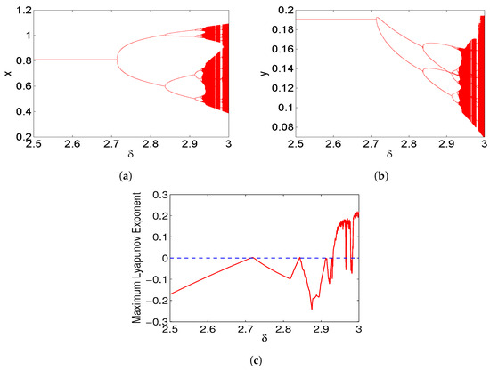
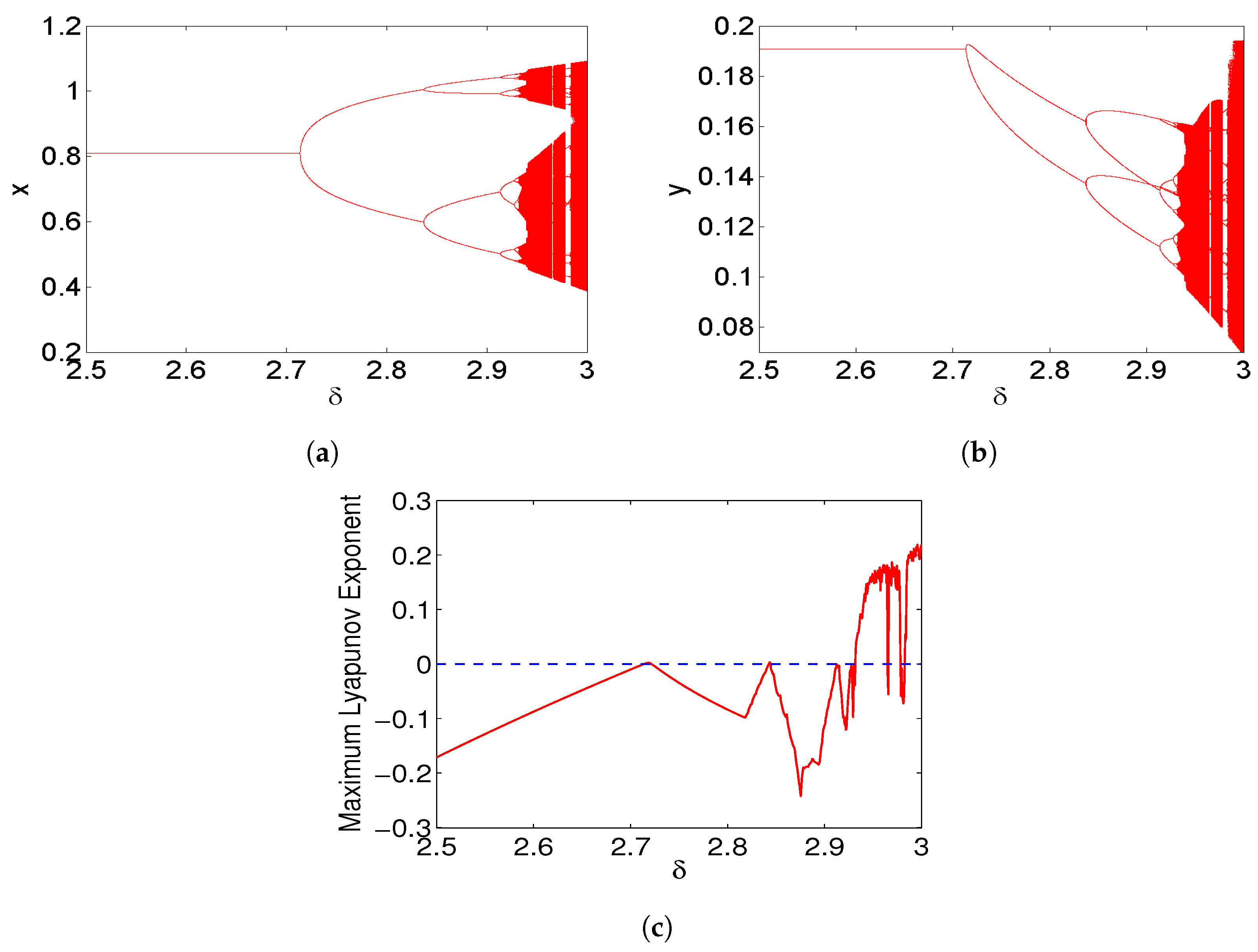
Fix $\gamma =1$, $m=1$, $\alpha =0.91$, $\beta =1$, since $0<\alpha <m\gamma$, then there is a unique positive fixed point $E_2(0.80918,0.19082)$ and we have ${\zeta }_1=-0.92254$, ${\zeta }_2=0.13673>0$, ${\lambda }_1=-1$, ${\lambda }_2\approx 0.49656$, satisfying $|{\lambda }_2|\ne 1$, ${\delta }_1={\displaystyle \frac{-{\zeta }_1-\sqrt{\Delta }}{{\zeta }_2}}\approx 2.71362$, ${\alpha }_1\approx -1.47405\ne 0$, ${\alpha }_2\approx 0.87499>0$. We can also easily obtain that ${\zeta }_1<-2\sqrt{{\zeta }_2}$, when $0<\delta <{\delta }_1$, and the conditions of Theorem 2 (I)(i) are satisfied. Hence, the fixed point $E_2(0.80918,0.19082)$ is a sink that is stable when $0<\delta <{\delta }_1$. According to Theorem 7, system (3) undergoes a supercritical flip bifurcation at $E_2(0.80918,0.19082)$ when δ crosses through the critical value ${\delta }_1$. That is, when $\delta >{\delta }_1$, $E_2(0.80918,0.19082)$ becomes unstable and a period-2 orbit appears as shown in Figure 4a,b. In addition, we observe a cascade of period-doublings. The maximum Lyapunov exponent has been computed and is shown in Figure 4c. The exponent implies that chaotic sets exist when $\delta ⪆2.93$. The phase portraits corresponding to Figure 4a,b are displayed in Figure 5. When δ is in the range of $(2.71362,2.93)$, there are orbits with periods of 2, 4, 8, and 16, and when $\delta ⪆2.93$, the chaotic sets can be seen.

Figure 4. (a) A bifurcation diagram in the $(\delta ,x)$ plane. (b) A bifurcation diagram in the $(\delta ,y)$ plane. (c) The maximum Lyapunov exponent corresponding to (a,b). Here, the values are set as follows: $\gamma =1$, $m=1$, $\alpha =0.91$, $\beta =1$ and the initial value is $(0.8,0.2)$.

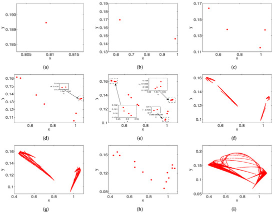
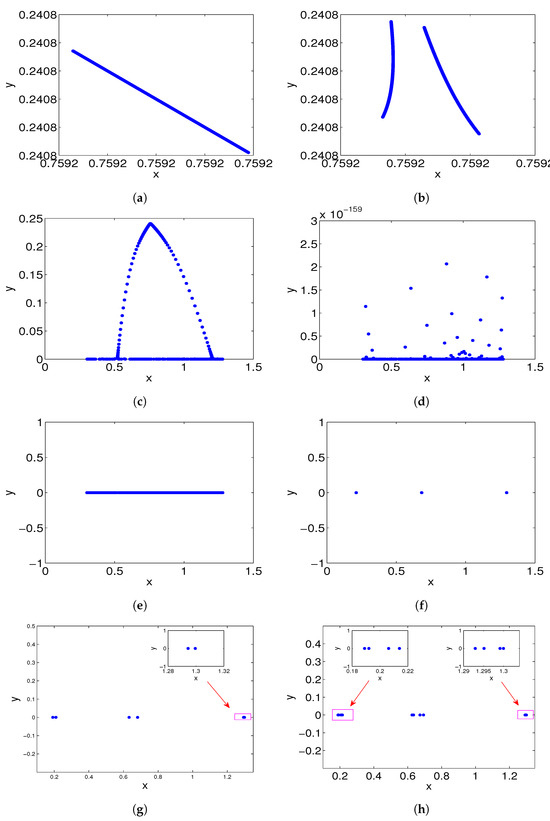
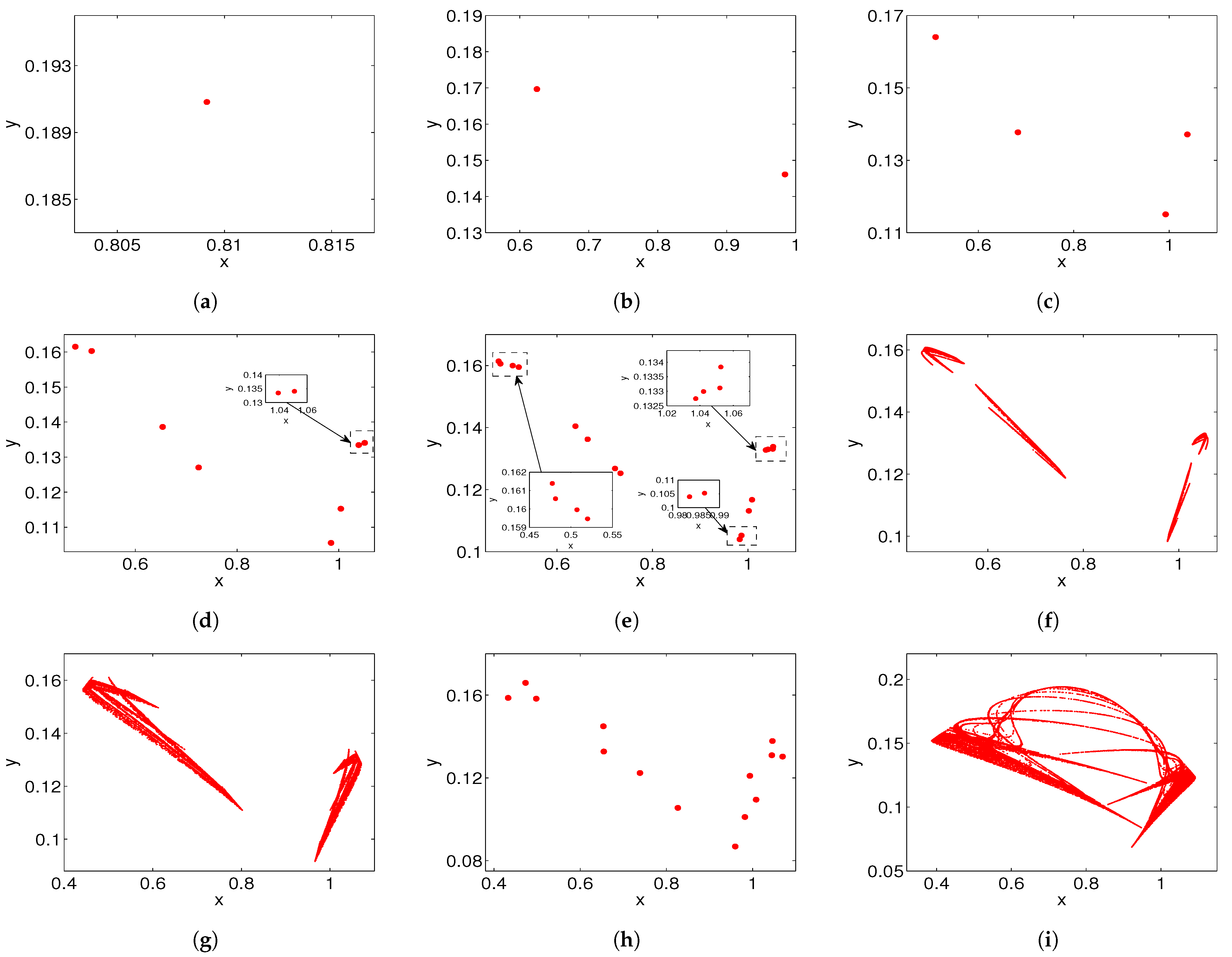
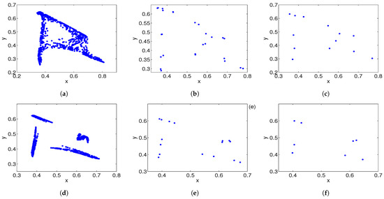
Figure 5. Phase portraits for different values of $\delta$ corresponding to Figure 4, with the initial value being $(0.8,0.2)$. (a) The phase portrait of the fixed point when $\delta =2.6$. (b) The phase portrait of the period-2 when $\delta =2.8$. (c) The phase portrait of the period-4 when $\delta =2.9$. (d) The phase portrait of the period-8 when $\delta =2.926$. (e) The phase portrait of the period-16 when $\delta =2.93$. (f) The chaotic set when $\delta =2.93$. (g) The chaotic set when $\delta =2.95$. (h) The phase portrait of the period-14 when $\delta =2.98$. (i) The chaotic set when $\delta =3.00$.

3.5. Neimark–Sacker Bifurcation around the Positive Fixed Points $E_k$

Next, we will utilize the bifurcation theorem [39,40] to discuss the Neimark–Sacker bifurcation of system (3). The result of this subsection is partly dependent on the following Lemma 3.

Lemma 3.

Let $F_{\alpha }$ be a one parameter family of map of ${\mathbb{R}}^2$ satisfying

(i)

$F_{\alpha }\left(0\right)=0$ for α near 0;

(ii)

$D{F}_{\alpha }\left(0\right)$ has two complex eigenvalues $\lambda \left(\alpha \right)$, $\overline{\lambda }\left(\alpha \right)$ for α near 0 with $\left|\lambda \right(0\left)\right|=1$;

(iii)

${\displaystyle \frac{\mathrm{d}\left|\lambda \right(\alpha \left)\right|}{\mathrm{d}\alpha }}{|}_{\alpha =0}>0$;

(iv)

$\lambda =\lambda \left(0\right)$ is not an mth root of unity for $m=1,2,3,4$.

Then, there is a smooth α-dependent change in coordinates, bringing $F_{\alpha }$ into the form

$$F_{\alpha }\left(X\right)=G_{\alpha }\left(U\right)+{\mathcal{O}\left(\right|U|}^5),$$

where $U\in {\mathbb{R}}^2$, $U=(u,v)$ and $G=(g_1,g_2)$.

Moreover, for all sufficiently small positive (negative) α, $F_{\alpha }$ has an attracting (repelling) invariant circle if $l\left(0\right)<0$ ($l\left(0\right)>0$), respectively, and $l\left(0\right)$ is given by following formula

$$l\left(0\right)=-\mathrm{Re}\left[{\displaystyle \frac{(1-2\lambda ){\overline{\lambda }}^2}{1-\lambda }}{\gamma }_{20}{\gamma }_{11}\right]-{\displaystyle \frac{1}{2}}|{\gamma }_{11}{|}^2-{\left|{\gamma }_{02}\right|}^2+\mathrm{Re}\left(\overline{\lambda }{\gamma }_{21}\right),$$

where

$$\begin{array}{c}{\gamma }_{20}={\displaystyle \frac{1}{8}}\left[(g_{1uu}-g_{1vv}+2g_{2uv})+\mathrm{i}(g_{2uu}-g_{2vv}-2g_{1uv})\right],\hfill \\ {\gamma }_{11}={\displaystyle \frac{1}{4}}\left[(g_{1uu}+g_{1vv})+\mathrm{i}(g_{2uu}+g_{2vv})\right],\hfill \\ {\gamma }_{02}={\displaystyle \frac{1}{8}}\left[(g_{1uu}-g_{1vv}-2g_{2uv})+\mathrm{i}(g_{2uu}-g_{2vv}+2g_{1uv})\right],\hfill \\ {\gamma }_{21}={\displaystyle \frac{1}{16}}\left[(g_{1uuu}+g_{1uvv}+g_{2uuv}+g_{2vvv})+\mathrm{i}(g_{2uuu}+g_{2uvv}-g_{1uuv}-g_{1vvv})\right].\hfill \end{array}$$

From Theorem 1, the eigenvalues of the boundary fixed point $E_0(1,0)$ are ${\lambda }_1=1+m\delta -{\displaystyle \frac{\alpha \delta }{\gamma }}$, ${\lambda }_2=1-\delta$. $E_0$ does not have two complex eigenvalues. Hence, according to bifurcation theorem, system (3) can not undergo a Neimark–Sacker bifurcation at $E_0(1,0)$.

Recall that Theorem 3 (III), the fixed point $E_k(x_k,y_k)$$(k=1,2,3)$ may undergo a Neimark–Sacker bifurcation when ${\zeta }_{2k}>0$, $-2\sqrt{{\zeta }_{2k}}<{\zeta }_{1k}<0$ and $\delta =\overline{\delta }=-{\displaystyle \frac{{\zeta }_{1k}}{{\zeta }_{2k}}}$. That is $\Delta =p^2\left(\delta \right)-4q\left(\delta \right)={\left(-{\zeta }_{1k}\delta -2\right)}^2-4\left({\zeta }_{2k}{\delta }^2+{\zeta }_{1k}\delta +1\right)={\delta }^2\left({\zeta }_{1k}^2-4{\zeta }_{2k}\right)<0$; hence, the eigenvalues of the characteristic Equation (6) evaluated at the positive fixed point $E_k(x_k,y_k)$ are

$$\begin{array}{c}{\lambda }_{1,2}\left(\delta \right)={\displaystyle \frac{-p\left(\delta \right)\pm \sqrt{p^2\left(\delta \right)-4q\left(\delta \right)}}{2}}={\displaystyle \frac{-p\left(\delta \right)\pm \mathrm{i}\sqrt{4q\left(\delta \right)-p^2\left(\delta \right)}}{2}},\hfill \end{array}$$

where ${\mathrm{i}}^2=-1$. Then

$$\begin{array}{c}|{\lambda }_{1,2}\left(\delta \right)|=\sqrt{{\left({\displaystyle \frac{-p\left(\delta \right)}{2}}\right)}^2+{\left({\displaystyle \frac{\sqrt{4q\left(\delta \right)-p{\left(\delta \right)}^2}}{2}}\right)}^2}=\sqrt{q\left(\delta \right)},\hfill \end{array}$$

hence $|{\lambda }_{1,2}\left(\overline{\delta }\right)|=\sqrt{q\left(\overline{\delta }\right)}=\sqrt{{\zeta }_{2k}{\left(-{\displaystyle \frac{{\zeta }_{1k}}{{\zeta }_{2k}}}\right)}^2+{\zeta }_{1k}\left(-{\displaystyle \frac{{\zeta }_{1k}}{{\zeta }_{2k}}}\right)+1}$ = 1.

Furthermore, due to ${\zeta }_{1k}<0$, the transversality condition

$$\begin{array}{c}d={\displaystyle \frac{\mathrm{d}|{\lambda }_{1,2}\left(\delta \right)|}{\mathrm{d}\delta }}{|}_{\delta =\overline{\delta }}={\displaystyle \frac{2{\zeta }_{2k}\delta +{\zeta }_{1k}}{2\sqrt{{\zeta }_{2k}{\delta }^2+{\zeta }_{1k}\delta +1}}}{|}_{\delta =\overline{\delta }}={\displaystyle \frac{2{\zeta }_{2k}\overline{\delta }+{\zeta }_{1k}}{2}}=-{\displaystyle \frac{{\zeta }_{1k}}{2}}>0.\hfill \end{array}$$

Furthermore, if $p\left(\overline{\delta }\right)$ is neither 0 nor 1, this will cause

$$\begin{array}{c}\overline{\delta }\ne -{\displaystyle \frac{2}{{\zeta }_{1k}}}\mathrm{and}\overline{\delta }\ne -{\displaystyle \frac{3}{{\zeta }_{1k}}},\hfill \end{array}$$

(26)

then we have ${\lambda }_{1,2}^n\left(\overline{\delta }\right)\ne 1$, $n=1,2,3,4$.

Next, we will verify the other non-degeneracy condition of Neimark–Sacker bifurcation. Letting $u_n=x_n-x_k$, $v_n=y_n-y_k$, we turn the fixed point $(x_k,y_k)$ into $O(0,0)$ and carry out an expansion on the right-hand side of Equation (3)

$$\left\{\begin{array}{c}{u}_{n+1}=(1-\delta x_k)u_n-\delta x_k{v}_n-\delta u_n^2-\delta u_n{v}_n,\hfill \\ v_{n+1}={\displaystyle \frac{\beta \delta y_k^2}{x_k^2}}{u}_n+(1+\delta m-{\displaystyle \frac{\delta \gamma \alpha }{{(\gamma +y_k)}^2}}-{\displaystyle \frac{2\beta \delta y_k}{x_k}})v_n-{\displaystyle \frac{\beta \delta y_k^2}{x_k^3}}{u}_n^2+{\displaystyle \frac{2\beta \delta y_k}{x_k^2}}{u}_n{v}_n+\left({\displaystyle \frac{\delta \gamma \alpha }{{(\gamma +y_k)}^3}}-{\displaystyle \frac{\beta \delta }{x_k}}\right)v_n^2\hfill \\ +{\displaystyle \frac{\beta \delta y_k^2}{x_k^4}}{u}_n^3-{\displaystyle \frac{2\beta \delta y_k}{x_k^3}}{u}_n^2{v}_n+{\displaystyle \frac{\beta \delta }{x_k^2}}{u}_n{v}_n^2-{\displaystyle \frac{\delta \gamma \alpha }{{(\gamma +y_k)}^4}}{v}_n^3+\mathcal{O}\left(\parallel (u_n,v_n){\parallel }^4\right).\hfill \end{array}\right.$$

(27)

Let

$$T=\left(\begin{array}{cc}-\delta x_k& 0\\ -{\displaystyle \frac{1}{2}}p-1+\delta x_k& -{\displaystyle \frac{\sqrt{4q-p^2}}{2}}\end{array}\right),$$

and use the translation

$$\left(\begin{array}{c}{u}_n\\ v_n\end{array}\right)=T\left(\begin{array}{c}{\phi }_n\\ {\psi }_n\end{array}\right),$$

(28)

then map (28) becomes

$$\left(\begin{array}{c}{\phi }_{n+1}\\ {\psi }_{n+1}\end{array}\right)=\left(\begin{array}{cc}-{\displaystyle \frac{p}{2}}& -{\displaystyle \frac{\sqrt{4q-p^2}}{2}}\\ {\displaystyle \frac{\sqrt{4q-p^2}}{2}}& -{\displaystyle \frac{p}{2}}\end{array}\right)\left(\begin{array}{c}{\phi }_n\\ {\psi }_n\end{array}\right)+\left(\begin{array}{c}\widehat{f}\left({\phi }_n,{\psi }_n\right)\\ \widehat{g}\left({\phi }_n,{\psi }_n\right)\end{array}\right),$$

(29)

where

$$\begin{array}{cc}\widehat{f}\left({\phi }_n,{\psi }_n\right)\hfill & ={\displaystyle \frac{1}{2}}\delta (p+2){\phi }_n^2+{\displaystyle \frac{1}{2}}\delta \sqrt{4q-p^2}{\phi }_n{\psi }_n,\hfill \\ \widehat{g}\left({\phi }_n,{\psi }_n\right)\hfill & =\left({\displaystyle \frac{\delta \alpha \gamma {(2-2\delta x_k+p)}^2}{2{(\gamma +y_k)}^3\sqrt{4q-p^2}}}-{\displaystyle \frac{4\beta {\delta }^3(x_k-2y_k)-2{\delta }^2(x_k+2\beta )(p+2)+\delta {(p+2)}^2}{2\sqrt{4q-p^2}}}+{\displaystyle \frac{(4{\delta }^2{y}_k^2-4\delta y_k(p+2)-{(p+2)}^2)\beta \delta }{2x_k\sqrt{4q-p^2)}}}\right){\phi }_n^2\hfill \\ \hfill & +\left({\delta }^2{x}_k-{\displaystyle \frac{\beta \delta (2\delta y_k+p+2)}{x_k}}+2\beta {\delta }^2-\delta -{\displaystyle \frac{1}{2}}\delta p+{\displaystyle \frac{\delta \gamma \alpha (2-2\delta x_k+p)}{{(\gamma +y_k)}^3}}\right){\phi }_n{\psi }_n\hfill \\ \hfill & +\left({\displaystyle \frac{\delta \alpha \gamma \sqrt{4q-p^2}}{2{(\gamma +y_k)}^3}}-{\displaystyle \frac{\beta \delta \sqrt{4q-p^2}}{2x_k}}\right){\psi }_n^2+\left({\displaystyle \frac{\beta {\delta }^2(2-2\delta y_k+p)}{x_k}}-2\beta {\delta }^3-{\displaystyle \frac{3\delta \gamma \alpha {(2-2\delta x_k+p)}^2}{4{(\gamma +y_k)}^4}}\right){\phi }_n^2{\psi }_n\hfill \\ \hfill & +\left({\displaystyle \frac{\beta {\delta }^2\sqrt{4q-p^2}}{2x_k}}-{\displaystyle \frac{3\delta \alpha \gamma (2-2\delta x_k+p)\sqrt{4q-p^2}}{4{(\gamma +y_k)}^4}}\right){\phi }_n{\psi }_n^2+{\displaystyle \frac{\delta \alpha \gamma (p^2-4q)}{4{(\gamma +y_k)}^4}}{\psi }_n^3\hfill \\ \hfill & +\left({\displaystyle \frac{\beta {\delta }^2{(2-2\delta y_k+p)}^2}{2\sqrt{4q-p^2}{x}_k}}-{\displaystyle \frac{2\beta {\delta }^3(p+2-\delta (x_k+2y_k))}{\sqrt{4q-p^2}}}-{\displaystyle \frac{\delta \alpha \gamma {(2-2\delta x_k+p)}^3}{4\sqrt{4q-p^2}{(\gamma +y_k)}^4}}\right){\phi }_n^3+\mathcal{O}\left(\parallel ({\phi }_n,{\psi }_n){\parallel }^4\right),\hfill \end{array}$$

For map (29) to undergo a Neimark–Sacker bifurcation, the following coefficient $l\left(0\right)$ must not be zero and

$$l\left(0\right)=-\mathrm{Re}\left[{\displaystyle \frac{\left(1-2\lambda \right){\overline{\lambda }}^2}{1-\lambda }}{\vartheta }_{11}{\vartheta }_{20}\right]-{\displaystyle \frac{1}{2}}|{\vartheta }_{11}{|}^2-{\left|{\vartheta }_{02}\right|}^2+\mathrm{Re}\left(\overline{\lambda }{\vartheta }_{21}\right),$$

where

$$\begin{array}{c}{\vartheta }_{11}={\displaystyle \frac{1}{4}}\left[\left({\widehat{f}}_{{\phi }_n{\phi }_n}+{\widehat{f}}_{{\psi }_n{\psi }_n}\right)+\mathrm{i}\left(\phantom{\widehat{f}}{\widehat{g}}_{{\phi }_n{\phi }_n}+{\widehat{g}}_{{\psi }_n{\psi }_n}\right)\right],\hfill \\ {\vartheta }_{20}={\displaystyle \frac{1}{8}}\left[\left({\widehat{f}}_{{\phi }_n{\phi }_n}-{\widehat{f}}_{{\psi }_n{\psi }_n}+2{\widehat{g}}_{{\phi }_n{\psi }_n}\right)+\mathrm{i}\left({\widehat{g}}_{{\phi }_n{\phi }_n}-{\widehat{g}}_{{\psi }_n{\psi }_n}-2{\widehat{f}}_{{\phi }_n{\psi }_n}\right)\right],\hfill \\ {\vartheta }_{02}={\displaystyle \frac{1}{8}}\left[\left({\widehat{f}}_{{\phi }_n{\phi }_n}-{\widehat{f}}_{{\psi }_n{\psi }_n}-2{\widehat{g}}_{{\phi }_n{\psi }_n}\right)+\mathrm{i}\left({\widehat{g}}_{{\phi }_n{\phi }_n}-{\widehat{g}}_{{\psi }_n{\psi }_n}+2{\widehat{f}}_{{\phi }_n{\psi }_n}\right)\right]\hfill \end{array}$$

and

$$\begin{array}{c}{\vartheta }_{21}={\displaystyle \frac{1}{16}}\left[\left({\widehat{f}}_{{\phi }_n{\phi }_n{\phi }_n}+{\widehat{f}}_{{\phi }_n{\psi }_n{\psi }_n}+{\widehat{g}}_{{\phi }_n{\phi }_n{\psi }_n}+{\widehat{g}}_{{\psi }_n{\psi }_n{\psi }_n}\right)+\mathrm{i}\left({\widehat{g}}_{{\phi }_n{\phi }_n{\phi }_n}+{\widehat{g}}_{{\phi }_n{\psi }_n{\psi }_n}-{\widehat{f}}_{{\phi }_n{\phi }_n{\psi }_n}-{\widehat{f}}_{{\psi }_n{\psi }_n{\psi }_n}\right)\right].\hfill \end{array}$$

Thus, by some computations we have

$$\begin{array}{c}l\left(0\right)={\displaystyle \frac{M_1}{32}}\left[{\widehat{g}}_{{\phi }_n{\phi }_n}^2-{\widehat{g}}_{{\psi }_n{\psi }_n}^2-2({\widehat{g}}_{{\psi }_n{\psi }_n}+{\widehat{g}}_{{\phi }_n{\phi }_n}){\widehat{f}}_{{\phi }_n{\psi }_n}-{\widehat{f}}_{{\phi }_n{\phi }_n}^2-2{\widehat{f}}_{{\phi }_n{\phi }_n}{\widehat{g}}_{{\phi }_n{\psi }_n}\right]\hfill \\ +{\displaystyle \frac{M_2}{16}}\left[\left({\widehat{f}}_{{\phi }_n{\phi }_n}+{\widehat{g}}_{{\phi }_n{\psi }_n}\right){\widehat{g}}_{{\phi }_n{\phi }_n}-{\widehat{f}}_{{\phi }_n{\phi }_n}{\widehat{f}}_{{\phi }_n{\psi }_n}+{\widehat{g}}_{{\psi }_n{\psi }_n}{\widehat{g}}_{{\phi }_n{\psi }_n}\right]-{\displaystyle \frac{p}{32}}({\widehat{g}}_{{\phi }_n{\phi }_n{\psi }_n}+{\widehat{g}}_{{\psi }_n{\psi }_n{\psi }_n})\hfill \\ +{\displaystyle \frac{\sqrt{4q-p^2}}{32}}\left({\widehat{g}}_{{\phi }_n{\phi }_n{\phi }_n}+{\widehat{g}}_{{\phi }_n{\psi }_n{\psi }_n}\right)-{\displaystyle \frac{3}{64}}{\widehat{g}}_{{\phi }_n{\phi }_n}^2-{\displaystyle \frac{1}{32}}(2{\widehat{f}}_{{\phi }_n{\psi }_n}+{\widehat{g}}_{{\psi }_n{\psi }_n}){\widehat{g}}_{{\phi }_n{\phi }_n}-{\displaystyle \frac{1}{16}}{\widehat{f}}_{{\phi }_n{\psi }_n}^2\hfill \\ +{\displaystyle \frac{1}{16}}{\widehat{f}}_{{\phi }_n{\psi }_n}{\widehat{g}}_{{\psi }_n{\psi }_n}-{\displaystyle \frac{3}{64}}{\widehat{f}}_{{\phi }_n{\phi }_n}^2+{\displaystyle \frac{1}{16}}{\widehat{f}}_{{\phi }_n{\phi }_n}{\widehat{g}}_{{\phi }_n{\psi }_n}-{\displaystyle \frac{3}{64}}{\widehat{g}}_{{\psi }_n{\psi }_n}^2-{\displaystyle \frac{1}{16}}{\widehat{g}}_{{\phi }_n{\psi }_n}^2,\hfill \end{array}$$

where

$$\begin{array}{c}{M}_1={\displaystyle \frac{(p^3+(2q+1)p^2-pq-4q^2-2q)}{2(q+p+1)}},M_2={\displaystyle \frac{(p^2+(2q+1)p+q)\sqrt{4q-p^2}}{2(q+p+1)}},\hfill \\ {\widehat{f}}_{{\phi }_n{\phi }_n}=\delta (p+2),{\widehat{f}}_{{\phi }_n{\psi }_n}={\displaystyle \frac{1}{2}}\delta \sqrt{4q-p^2},{\widehat{g}}_{{\psi }_n{\psi }_n}={\displaystyle \frac{\delta \alpha \gamma \sqrt{4q-p^2}}{{(\gamma +y_k)}^3}}-{\displaystyle \frac{\beta \delta \sqrt{4q-p^2}}{x_k}},\hfill \\ {\widehat{g}}_{{\phi }_n{\phi }_n}={\displaystyle \frac{\beta \delta (4{\delta }^2{y}_k^2-4\delta y_k(p+2)-{(p+2)}^2)}{x_k\sqrt{4q-p^2}}}-{\displaystyle \frac{4\beta {\delta }^3(x_k-2y_k)-2{\delta }^2(x_k+2\beta )(p+2)+\delta {(p+2)}^2}{\sqrt{4q-p^2}}}+{\displaystyle \frac{\delta \alpha \gamma {(2-2\delta x_k+p)}^2}{{(\gamma +y_k)}^3\sqrt{4q-p^2}}},\hfill \\ {\widehat{g}}_{{\phi }_n{\psi }_n}={\delta }^2{x}_k-{\displaystyle \frac{\beta \delta (2\delta y_k+p+2)}{x_k}}+2\beta {\delta }^2-\delta -{\displaystyle \frac{1}{2}}\delta p+{\displaystyle \frac{\delta \alpha \gamma (2-2\delta x_k+p)}{{(\gamma +y_k)}^3}},\hfill \\ {\widehat{g}}_{{\phi }_n{\phi }_n{\phi }_n}={\displaystyle \frac{3\beta {\delta }^2{(2-2\delta y_k+p)}^2}{x_k\sqrt{4q-p^2}}}-{\displaystyle \frac{12\beta {\delta }^3(2-(x_k+2y_k)\delta +p)}{\sqrt{4q-p^2}}}-{\displaystyle \frac{3\delta \alpha \gamma {(2-2\delta x_k+p)}^3}{2{(\gamma +y_k)}^4\sqrt{4q-p^2}}},\hfill \\ {\widehat{g}}_{{\phi }_n{\psi }_n{\psi }_n}={\displaystyle \frac{\beta {\delta }^2\sqrt{4q-p^2}}{x_k}}-{\displaystyle \frac{3\delta \alpha \gamma (2-2\delta x_k+p)\sqrt{4q-p^2}}{2{(\gamma +y_k)}^4}},{\widehat{g}}_{{\psi }_n{\psi }_n{\psi }_n}={\displaystyle \frac{3\delta \alpha \gamma (p^2-4q)}{2{(\gamma +y_k)}^4}},\hfill \\ {\widehat{g}}_{{\phi }_n{\phi }_n{\psi }_n}={\displaystyle \frac{2\beta {\delta }^2(2-2\delta y_k+p))}{x_k}}-4\beta {\delta }^3-{\displaystyle \frac{3\delta \alpha \gamma {(2-2\delta x_k+p)}^2}{2{(\gamma +y_k)}^4}}.\hfill \end{array}$$

Theorem 8.

Map (3) will undergo a Neimark–Sacker bifurcation at $E_k(x_k,y_k)$ when δ varies in a small neighborhood of $\overline{\delta }$, provided that the conditions ${\zeta }_{2k}>0$, $-2\sqrt{{\zeta }_{2k}}<{\zeta }_{1k}<0$, $\delta =\overline{\delta }=-{\displaystyle \frac{{\zeta }_{1k}}{{\zeta }_{2k}}}$$(k=1,2,3)$ and Equation (26) hold and $l\left(0\right)\ne 0$. Moreover, because $d={\displaystyle \frac{\mathrm{d}|{\lambda }_{1,2}\left(\delta \right)|}{\mathrm{d}\delta }}{|}_{\delta =\overline{\delta }}>0$, when $l\left(0\right)<0$ (resp. $l\left(0\right)>0$), an attracting (resp. repelling) invariant closed curve will bifurcate from the fixed point for $\delta >\overline{\delta }$ (resp. $\delta <\overline{\delta }$).

Example 5.

Fix $\gamma =1.3$, $m=2.5$, $\alpha =3.18133$, $\beta =0.5$, we have the fixed point $E_2(0.369896,$$0.630104)$, ${\zeta }_{12}=-0.683532<0$, ${\zeta }_{22}=0.652692>0$, the critical parameter value $\overline{\delta }=-{\displaystyle \frac{{\zeta }_{12}}{{\zeta }_{22}}}=1.047250$. Moreover, the eigenvalues $\lambda =0.642086\pm 0.766633\mathrm{i}$ and $l\left(0\right)=-0.5881410<0$. According to Theorem 8, a Neimark–Sacker bifurcation occurs in system (3) at $E_2(0.369896,0.630104)$.

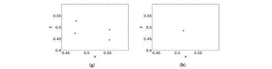
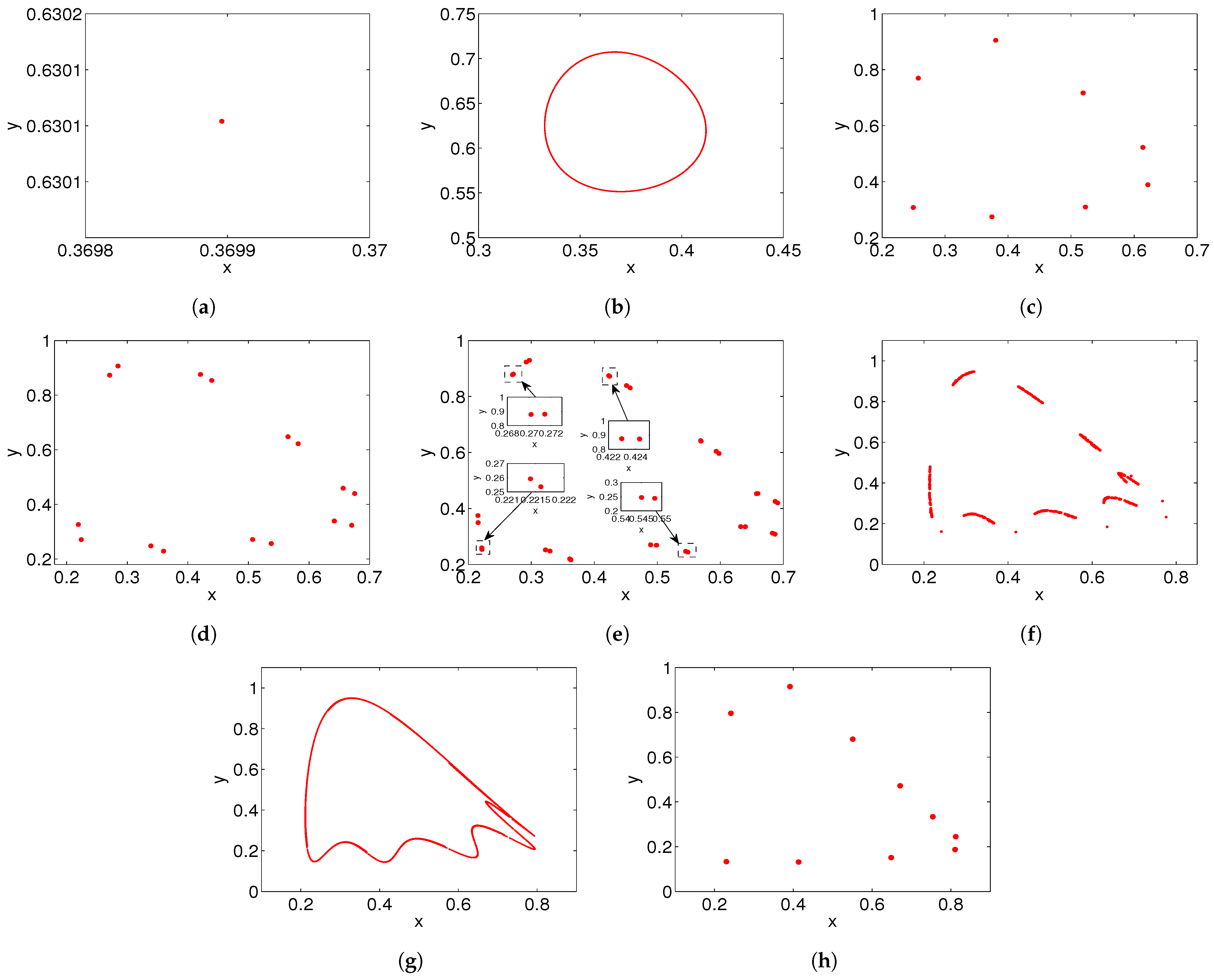
The bifurcation diagram of system (3) for $1\le \delta \le 1.4$ is presented in Figure 6a with a initial value $(x_0,y_0)=(0.7,0.3)$. When $1\le \delta <1.4$, there is a stable fixed point. As shown in Figure 6a, a Neimark–Sacker bifurcation occurs at $\delta ={\delta }^{*}=1.047250$ and an attracting invariant cycle bifurcates from the fixed point. The maximum Lyapunov exponents are in Figure 6b. As δ increases, the cycle first becomes bigger and then disappears. Then, system (3) has period-8, -10, -16, -32 orbits. The phase portraits are in Figure 7. In Figure 7e, there are a total of 8 clusters of point sets. Each cluster has four points. In each cluster, two points are difficult to distinguish. We have enlarged the two indistinguishable points in four of the clusters. For the remaining four clusters, we did not enlarge and display them again.

Figure 6. (a) A bifurcation diagram in the $(\delta ,x)$ plane. (b) The maximum Lyapunov exponent corresponding to (a).

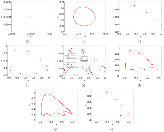
Figure 7. (a) There is a stable point when $\delta =1.04$. (b) There is a limit cycle when $\delta =1.05$. (c) There are period-8 points when $\delta =1.13$. (d) There are period-16 points when $\delta =1.2$. (e) There are period-32 points when $\delta =1.215$. (f) There is chaos when $\delta =1.23$. (g) There is chaos when $\delta =1.24$. (h) There are period-10 points when $\delta =1.25$.

4. Codimension 2 Bifurcations

4.1. Fold–Flip Bifurcation

In this subsection, we will consider the codimension 2 bifurcation of system (3) by choosing $\delta$ and m as bifurcation parameters. If $\delta =2$, $\alpha =m\gamma$ or $\delta =-{\displaystyle \frac{2}{{\zeta }_{1k}}}$$({\zeta }_{1k}<0)$, ${\zeta }_{2k}=0$, i.e., $\alpha ={\displaystyle \frac{2{(\gamma +y_1)}^2\left(-\frac{3}{2}\beta y_1^2+\left(\left(\frac{1}{2}m-2\beta \right)x_1+\beta \right)y_1+m{x}_1\left(x-\frac{1}{2}\right)\right)}{\gamma x_1(2x_1+y_1-1)}}$, there exist two critical eigenvalues ${\lambda }_1=1$, ${\lambda }_2=-1$ at the fixed point $E_0(1,0)$ or $E_1(x_1,y_1)$. From Theorem 1 (IV)(iv) or Theorem 3 (IV), a fold–flip bifurcation may occur at $E_0$ or $E_1$. For simplicity, let $E^{*}(x^{*},y^{*})$ denote the fixed point $E_1(x_1,y_1)$ or $E_0(1,0)$, ${\delta }^{*}$ denote 2 or $-{\displaystyle \frac{2}{{\zeta }_{1k}}}$, and ${\alpha }^{*}$ denote $m\gamma$ or ${\displaystyle \frac{2{(\gamma +y_1)}^2\left(-\frac{3}{2}\beta y_1^2+\left(\left(\frac{1}{2}m-2\beta \right)x_1+\beta \right)y_1+m{x}_1\left(x-\frac{1}{2}\right)\right)}{\gamma x_1(2x_1+y_1-1)}}$.

Let $u_{1,n}=x_n-x^{*}$, $u_{2,n}=y_n-y^{*}$, $\widehat{\delta }=\delta -{\delta }^{*}$, and $\widehat{\alpha }=\alpha -{\alpha }^{*}$. Then, we transform $E^{*}(x^{*},y^{*})$ to $O(0,0)$ and expand the right-hand side of system (3)

$$\left(\begin{array}{c}{u}_{1,n+1}\\ u_{2,n+1}\end{array}\right)=\left(\begin{array}{cc}1-{\delta }^{*}{b}_{11}& -{\delta }^{*}{b}_{12}\\ {\delta }^{*}{b}_{21}& 1+{\delta }^{*}{b}_{22}\end{array}\right)\left(\begin{array}{c}{u}_{1,n}\\ u_{2,n}\end{array}\right)+\left(\begin{array}{c}-b_{11}\widehat{\delta }{u}_{1,n}-b_{12}\widehat{\delta }{u}_{2,n}+f\left(u_{1,n},u_{2,n}\right)\\ L_2+b_{21}\widehat{\delta }{u}_{1,n}-b_{22}\widehat{\delta }{u}_{2,n}-b_{23}\widehat{\delta }\widehat{\alpha }{u}_{2,n}+g\left(u_{1,n},u_{2,n}\right)\end{array}\right),$$

(30)

where

$$\begin{array}{c}{b}_{11}=b_{12}=x^{*},b_{21}={\displaystyle \frac{\beta y^{*2}}{x^{*2}}},b_{22}=m-{\displaystyle \frac{2\beta y^{*}}{x^{*}}}-{\displaystyle \frac{\gamma (\widehat{\alpha }+{\alpha }^{*})}{{(\gamma +y^{*})}^2}},L_2=-{\displaystyle \frac{\widehat{\alpha }{y}^{*}\left(\widehat{\delta }+{\delta }^{*}\right)}{\gamma +y^{*}}},\hfill \\ f(u_{1,n},u_{2,n})=-\left(\widehat{\delta }+{\delta }^{*}\right)u_{1,n}^2-\left(\widehat{\delta }+{\delta }^{*}\right)u_{1,n}{u}_{2,n},\hfill \\ g(u_{1,n},u_{2,n})=-{\displaystyle \frac{\beta y^{*2}\left(\widehat{\delta }+{\delta }^{*}\right)}{x^{*3}}}{u}_{1,n}^2+{\displaystyle \frac{2\beta \left(\widehat{\delta }+{\delta }^{*}\right)y^{*}}{x^{*2}}}{u}_{1,n}{u}_{2,n}+\left({\displaystyle \frac{\gamma \left(\widehat{\delta }+{\delta }^{*}\right)\left(\widehat{\alpha }+{\alpha }^{*}\right)}{{(\gamma +y^{*})}^3}}-{\displaystyle \frac{\gamma \widehat{\alpha }\widehat{\delta }}{{\left(\gamma +y^{*}\right)}^3}}-{\displaystyle \frac{\beta \left(\widehat{\delta }+{\delta }^{*}\right)}{x^{*}}}\right)u_{2,n}^2\hfill \\ -{\displaystyle \frac{2\beta {\delta }^{*}{y}^{*}}{x^{*3}}}{u}_{1,n}^2{u}_{2,n}+{\displaystyle \frac{\beta {\delta }^{*}}{x^{*2}}}{u}_{1,n}{u}_{2,n}^2-{\displaystyle \frac{{\delta }^{*}{\alpha }^{*}\gamma }{{(\gamma +y^{*})}^4}}{u}_{2,n}^3+{\displaystyle \frac{\beta {\delta }^{*}{y}^{*2}}{x^{*4}}}{u}_{1,n}^3+\mathcal{O}\left(\parallel (u_{1,n},u_{2,n}){\parallel }^4\right).\hfill \end{array}$$

For simplicity, let $\kappa ={\left(\widehat{\delta },\widehat{\alpha }\right)}^T$. We construct a matrix $T_1=\left(\begin{array}{cc}{b}_{12}& -{\delta }^{*}{b}_{12}\\ -b_{11}& -2+{\delta }^{*}{b}_{11}\end{array}\right)$, with the non-singular linear coordinate transformation

$$\left(\begin{array}{c}{u}_{1,n}\\ u_{2,n}\end{array}\right)=T_1\left(\begin{array}{c}{v}_{1,n}\\ v_{2,n}\end{array}\right).$$

(31)

system (30) can be written as

$$\left(\begin{array}{c}{v}_{1,n+1}\\ v_{2,n+1}\end{array}\right)={\Lambda }_0\left(\kappa \right)+{\Lambda }_1\left(\kappa \right)\left(\begin{array}{c}{v}_{1,n}\\ v_{2,n}\end{array}\right)+\left(\begin{array}{c}{f}_1\left(v_{1,n},v_{2,n}\right)\\ g_1\left(v_{1,n},v_{2,n}\right)\end{array}\right),$$

(32)

where

$$\begin{array}{c}{\Lambda }_0\left(\kappa \right)=\left(\begin{array}{c}-{\displaystyle \frac{{\delta }^{*}}{2}}{L}_2\\ -{\displaystyle \frac{1}{2}}{L}_2\end{array}\right),\hfill \\ {\Lambda }_1\left(\kappa \right)=\left(\begin{array}{cc}1& \widehat{\delta }[2+{\delta }^{*}(b_{22}-b_{11})]\\ 0& -1+\widehat{\delta }(b_{22}-b_{11})\end{array}\right),\hfill \\ f_1(v_{1,n},v_{2,n})=f_{20}{v}_{1,n}^2+f_{11}{v}_{1,n}{v}_{2,n}+f_{02}{v}_{2,n}^2+f_{30}{v}_{1,n}^3+f_{21}{v}_{1,n}^2{v}_{2,n}+f_{12}{v}_{1,n}{v}_{2,n}^2\hfill \\ +f_{03}{v}_{2,n}^3+\mathcal{O}\left(\parallel (v_{1,n},v_{2,n}){\parallel }^4\right),\hfill \\ g_1(v_{1,n},v_{2,n})=g_{20}{v}_{1,n}^2+g_{11}{v}_{1,n}{v}_{2,n}+g_{02}{v}_{2,n}^2+g_{30}{v}_{1,n}^3+g_{21}{v}_{1,n}^2{v}_{2,n}+g_{12}{v}_{1,n}{v}_{2,n}^2\hfill \\ +g_{03}{v}_{2,n}^3+\mathcal{O}\left(\parallel (v_{1,n},v_{2,n}){\parallel }^4\right).\hfill \end{array}$$

(33)

and the coefficients of $f_1(v_{1,n},v_{2,n})$ and $g_1(v_{1,n},v_{2,n})$ are given in Appendix E.

The eigenvectors of ${\Lambda }_1\left(\kappa \right)$ corresponding to the eigenvalues ${\lambda }_1\left(\kappa \right)=1$ and ${\lambda }_2\left(\kappa \right)=-1+{\delta }^{*}(b_{22}-b_{11})$ are $q_0\left(\kappa \right)={\left(1,0\right)}^T$ and $q_1\left(\kappa \right)={\left(\widehat{\delta }[2+{\delta }^{*}(b_{22}-b_{11})],-2+\widehat{\delta }(b_{22}-b_{11})\right)}^T$, respectively, which satisfy ${\Lambda }_1\left(0\right)q_0\left(0\right)=q_0\left(0\right)$, ${\Lambda }_1\left(0\right)q_1\left(0\right)=-q_1\left(0\right)$. At the same time, the eigenvectors of ${\Lambda }_1{\left(\kappa \right)}^T$ corresponding to the eigenvalues ${\lambda }_1\left(\kappa \right)$ and ${\lambda }_2\left(\kappa \right)$ are $p_0\left(\kappa \right)={\left(1,-1\right)}^T$ and $p_1\left(\kappa \right)={\left(0,1\right)}^T$, which satisfy ${\Lambda }_1{\left(0\right)}^T{p}_0\left(0\right)=p_0\left(0\right)$ and ${\Lambda }_1{\left(0\right)}^T{p}_1\left(0\right)=-p_1\left(0\right)$. These four vectors satisfy the following equalities

$$⟨p_0,q_0⟩=⟨p_1,q_1⟩=1,⟨p_0,q_1⟩=⟨p_1,q_0⟩=0,$$

where $⟨.,.⟩$ is the standard scalar product in ${\mathbb{R}}^2$. Once $q_0$ and $q_1$ are chosen, any ${\varrho }_n={(v_{1,n},v_{2,n})}^T\in {\mathbb{R}}^2$ can be uniquely written as ${\varrho }_n=w_{1,n}{q}_0+w_{2,n}{q}_1$ with $(w_{1,n},w_{2,n})\in {\mathbb{R}}^2$. We can calculate $w_{1,n}$ and $w_{2,n}$ explicitly

$$w_{1,n}=⟨p_0,{\varrho }_n⟩,w_{2,n}=⟨p_1,{\varrho }_n⟩.$$

In the coordinates $(w_{1,n},w_{2,n})$, map (32) can be be written as

$$\left(\begin{array}{c}{w}_{1,n+1}\\ w_{2,n+1}\end{array}\right)=\phi (w_n,\kappa )=\left(\begin{array}{c}{\theta }_1\left(\kappa \right)\\ {\theta }_2\left(\kappa \right)\end{array}\right)+\left(\begin{array}{cc}1& 0\\ 0& -1+\widehat{\delta }(b_{22}-b_{11})\end{array}\right)\left(\begin{array}{c}{w}_{1,n}\\ w_{2,n}\end{array}\right)+\left(\begin{array}{c}F(w_{1,n},w_{2,n})\\ G(w_{1,n},w_{2,n})\end{array}\right),$$

(34)

where the expressions of ${\theta }_1\left(\kappa \right)$, ${\theta }_2\left(\kappa \right)$, $F(w_{1,n},w_{2,n})$ and $G(w_{1,n},w_{2,n})$ are given in Appendix F.

When $\kappa ={(0,0)}^T$, map (34) can be expressed as

$$\left(\begin{array}{c}{w}_{1,n+1}\\ w_{2,n+1}\end{array}\right)=\left(\begin{array}{cc}1& 0\\ 0& -1\end{array}\right)\left(\begin{array}{c}{w}_{1,n}\\ w_{2,n}\end{array}\right)+\left(\begin{array}{c}{\tilde{f}}_1(w_{1,n},w_{2,n})\\ {\tilde{g}}_1(w_{1,n},w_{2,n})\end{array}\right),$$

(35)

where

$$\begin{array}{c}{\tilde{f}}_1(w_{1,n},w_{2,n})={\tilde{f}}_{20}{w}_{1,n}^2+{\tilde{f}}_{11}{w}_{1,n}{w}_{2,n}+{\tilde{f}}_{02}{w}_{2,n}^2+{\tilde{f}}_{30}{w}_{1,n}^3+{\tilde{f}}_{21}{w}_{1,n}^2{w}_{2,n}+{\tilde{f}}_{12}{w}_{1,n}{w}_{2,n}^2\hfill \\ +{\tilde{f}}_{03}{w}_{2,n}^3+\mathcal{O}\left(\parallel (w_{1,n},w_{2,n}){\parallel }^4\right),\hfill \\ {\tilde{g}}_1(w_{1,n},w_{2,n})={\tilde{g}}_{20}{w}_{1,n}^2+{\tilde{g}}_{11}{v}_{1,n}{v}_{2,n}+{\tilde{g}}_{02}{v}_{2,n}^2+{\tilde{g}}_{30}{w}_{1,n}^3+{\tilde{g}}_{21}{w}_{1,n}^2{w}_{2,n}+{\tilde{g}}_{12}{w}_{1,n}{w}_{2,n}^2\hfill \\ +{\tilde{g}}_{03}{w}_{2,n}^3+\mathcal{O}\left(\parallel (w_{1,n},w_{2,n}){\parallel }^4\right),\hfill \\ {\tilde{f}}_{ij}=f_{ij}{{|}_{(\kappa =\mathbf{0})},{\tilde{g}}_{ij}=g_{ij}|}_{(\kappa =\mathbf{0})}.\hfill \end{array}$$

If

$$g_{11}\ne 0,$$

(36)

according to Proposition 2.1.1 in [41], near the origin, map (35) is smoothly equivalent to the map

$$\begin{array}{c}\left(\begin{array}{c}{x}_{1,n+1}\\ x_{2,n+1}\end{array}\right)\mapsto \left(\begin{array}{c}{x}_{1,n}+{\displaystyle \frac{1}{2}}a\left(0\right)x_{1,n}^2+{\displaystyle \frac{1}{2}}b\left(0\right)x_{2,n}^2+{\displaystyle \frac{1}{6}}c\left(0\right)x_{1,n}^3+{\displaystyle \frac{1}{2}}d\left(0\right)x_{1,n}{x}_{2,n}^2\\ -x_{2,n}+x_{1,n}{x}_{2,n}\end{array}\right)\hfill \\ +\mathcal{O}\left(\parallel (x_{1,n},x_{2,n}){\parallel }^4\right),\hfill \end{array}$$

(37)

where

$$\begin{array}{c}a\left(0\right)={\displaystyle \frac{2{\tilde{f}}_{20}}{{\tilde{g}}_{11}}},b\left(0\right)=2{\tilde{f}}_{02}{\tilde{g}}_{11},c\left(0\right)={\displaystyle \frac{1}{{\tilde{g}}_{11}^2}}(6{\tilde{f}}_{30}+3{\tilde{f}}_{11}{\tilde{g}}_{20}),\hfill \\ d\left(0\right)={\displaystyle \frac{3{\tilde{f}}_{02}(4{\tilde{g}}_{02}{\tilde{g}}_{20}+4{\tilde{g}}_{21}-4{\tilde{f}}_{11}{\tilde{g}}_{20})-{\tilde{f}}_{20}(12{\tilde{g}}_{02}^2+12{\tilde{g}}_{03})}{3{\tilde{g}}_{11}}}-{\tilde{f}}_{11}^2+2{\tilde{f}}_{12}+{\tilde{f}}_{11}{\tilde{g}}_{02}-4{\tilde{g}}_{02}^2-4{\tilde{g}}_{03}.\hfill \end{array}$$

Define $\left(\begin{array}{c}w\\ \kappa \end{array}\right)\mapsto \varphi (w,\kappa )=\left(\begin{array}{c}\phi (w,\kappa )-v\\ \mathrm{Det}{\phi }_w(w,\kappa )+1\\ \mathrm{Tr}{\phi }_w(w,\kappa )\end{array}\right),w=\left(\begin{array}{c}{w}_1\\ w_2\end{array}\right),\kappa =\left(\begin{array}{c}\widehat{\delta }\\ \widehat{\alpha }\end{array}\right).$ For map (34), we have

$${\displaystyle \frac{\partial \varphi }{\partial (w,\kappa )}}{|}_{(w=\kappa =\mathbf{0})}=\left(\begin{array}{cccc}0& 0& M_1& M_2\\ 0& -2& N_1& N_2\\ W_1+W_2& V_1+V_2& N_3& 0\\ W_1-W_2& V_1-V_2& N_3& 0\end{array}\right),$$

(38)

where

$$\begin{array}{c}{M}_1={\displaystyle \frac{{\tilde{b}}_{22}{\delta }^{*}+x^{*}{\delta }^{*}-2}{2}},M_2=-{\displaystyle \frac{{\delta }^{*2}{y}^{*}}{2(\gamma +y^{*})}},N_1={\displaystyle \frac{x^{*}+{\tilde{b}}_{22}}{2}},N_2=-{\displaystyle \frac{{\delta }^{*}{y}^{*}}{2(\gamma +y^{*})}},\hfill \\ W_1=-{\displaystyle \frac{{\delta }^{*2}({\delta }^{*}+1)}{16}}-{\displaystyle \frac{\beta [x^{*2}{\delta }^{*}-{\delta }^{*}(y^{*2}{\delta }^{*2}+2x^{*}{y}^{*}{\delta }^{*})]}{16x^{*3}}}+{\displaystyle \frac{{\delta }^{*}(2{\delta }^{*}+1)}{16x^{*}}}-{\displaystyle \frac{\beta y^{*}{\delta }^{*}(-y^{*}{\delta }^{*}+x^{*})}{8x^{*4}}}+{\displaystyle \frac{{\delta }^{*}{\alpha }^{*}\gamma }{16{(\gamma +y^{*})}^3}},\hfill \\ W_2={\displaystyle \frac{1}{4}}{\delta }^{*3}({\delta }^{*}+1)-{\displaystyle \frac{{\delta }^{*}(3x^{*2}{\delta }^{*2}+2x^{*2}{\delta }^{*}-6x^{*}{\delta }^{*}-2x^{*}+4)}{2x^{*3}}}+{\displaystyle \frac{{\delta }^{*2}\beta {(-y^{*}{\delta }^{*}+x^{*})}^2}{4x^{*3}}}-{\displaystyle \frac{\gamma {\alpha }^{*}{\delta }^{*2}}{4{(\gamma +y^{*})}^3}}+{\displaystyle \frac{\beta y^{*}{\delta }^{*2}(-x^{*}{y}^{*}{\delta }^{*}+x^{*2}+y^{*})}{x^{*5}}},\hfill \\ V_1=-{\displaystyle \frac{1}{4}}{\delta }^{*}\left\{-{\displaystyle \frac{1}{4}}{\delta }^{*2}({\delta }^{*}+1)+{\displaystyle \frac{4x^{*}{\delta }^{*2}+3x^{*}{\delta }^{*}-4{\delta }^{*}-2}{4x^{*2}}}-{\displaystyle \frac{{\delta }^{*}\beta {(-y^{*}{\delta }^{*}+x^{*})}^2}{4x^{*3}}}-{\displaystyle \frac{\beta y^{*}{\delta }^{*}(-y^{*}{\delta }^{*}+x^{*})}{2x^{*4}}}\right\}\hfill \\ +{\displaystyle \frac{1}{32}}{\delta }^{*2}({\delta }^{*}+1)+{\displaystyle \frac{{\delta }^{*}\beta {(-y^{*}{\delta }^{*}+x^{*})}^2}{32x^{*3}}}-{\displaystyle \frac{{\delta }^{*}{\alpha }^{*}\gamma }{32{(\gamma +y^{*})}^3}},\hfill \\ V_2={\displaystyle \frac{1}{4}}{\delta }^{*}\left\{-{\displaystyle \frac{1}{4}}{\delta }^{*2}({\delta }^{*}+1)+{\displaystyle \frac{4x^{*}{\delta }^{*2}+3x^{*}{\delta }^{*}-4{\delta }^{*}-2}{4x^{*2}}}-{\displaystyle \frac{{\delta }^{*}\beta {(-y^{*}{\delta }^{*}+x^{*})}^2}{4x^{*3}}}-{\displaystyle \frac{\beta y^{*}{\delta }^{*}(-y^{*}{\delta }^{*}+x^{*})}{2x^{*4}}}\right\},\hfill \\ N_3={\tilde{b}}_{22}-x^{*},{\tilde{b}}_{22}=m-{\displaystyle \frac{2\beta y^{*}}{x^{*}}}-{\displaystyle \frac{\gamma {\alpha }^{*}}{{(\gamma +y^{*})}^2}}.\hfill \end{array}$$

If

$$\mathrm{Det}\left({\displaystyle \frac{\partial \varphi }{\partial (w,\kappa )}}\right){|}_{w=\kappa =\mathbf{0}}\ne 0,$$

(39)

near the origin, map (34) is smoothly equivalent to a standard form of fold–flip bifurcation

$$\left\{\begin{array}{c}{x}_{1,n+1}={\mu }_1\left(\kappa \right)+(1+{\mu }_2\left(\kappa \right))x_{1,n}+{\displaystyle \frac{1}{2}}a\left(\kappa \right)x_{1,n}^2+{\displaystyle \frac{1}{2}}b\left(\kappa \right)x_{2,n}^2+{\displaystyle \frac{1}{6}}c\left(\kappa \right)x_{1,n}^3+{\displaystyle \frac{1}{2}}d\left(\kappa \right)x_{1,n}{x}_{2,n}^2,\hfill \\ x_{2,n+1}=-x_{2,n}+x_{1,n}{x}_{2,n}.\hfill \end{array}\right.$$

(40)

Theorem 9.

If $\delta =2$, $\alpha =m\gamma$, or $\delta =-{\displaystyle \frac{2}{{\zeta }_{1k}}}$$({\zeta }_{1k}<0)$, ${\zeta }_{2k}=0$, and conditions (36) and (39) hold, then map (3) undergoes a fold–flip bifurcation at $E^{*}$.

Example 6.

Fix $\gamma =2$, $m=1$, $\beta =0.8$. We have the critical parameter values ${\alpha }^{*}=2$, ${\delta }^{*}=2$ and the fixed point $E_0(1,0)$. The eigenvalues are ${\lambda }_{1,2}=\pm 1$ and $g_{11}=0.006105\ne 0$, $\mathrm{Det}\left({\displaystyle \frac{\partial \varphi }{\partial (w,\kappa )}}\right){|}_{w=\kappa =\mathbf{0}}=6.770433\ne 0$. According to Theorem 9, $E_0$ is a fold–flip point.

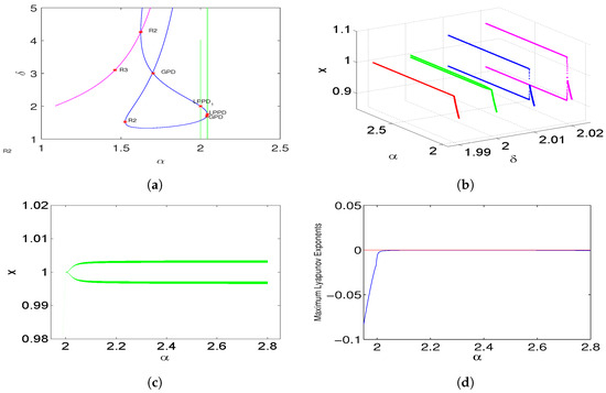
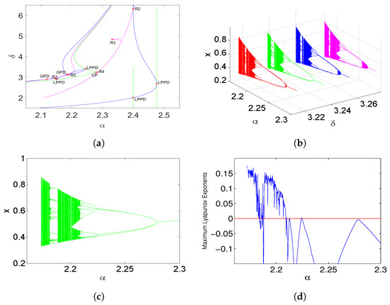
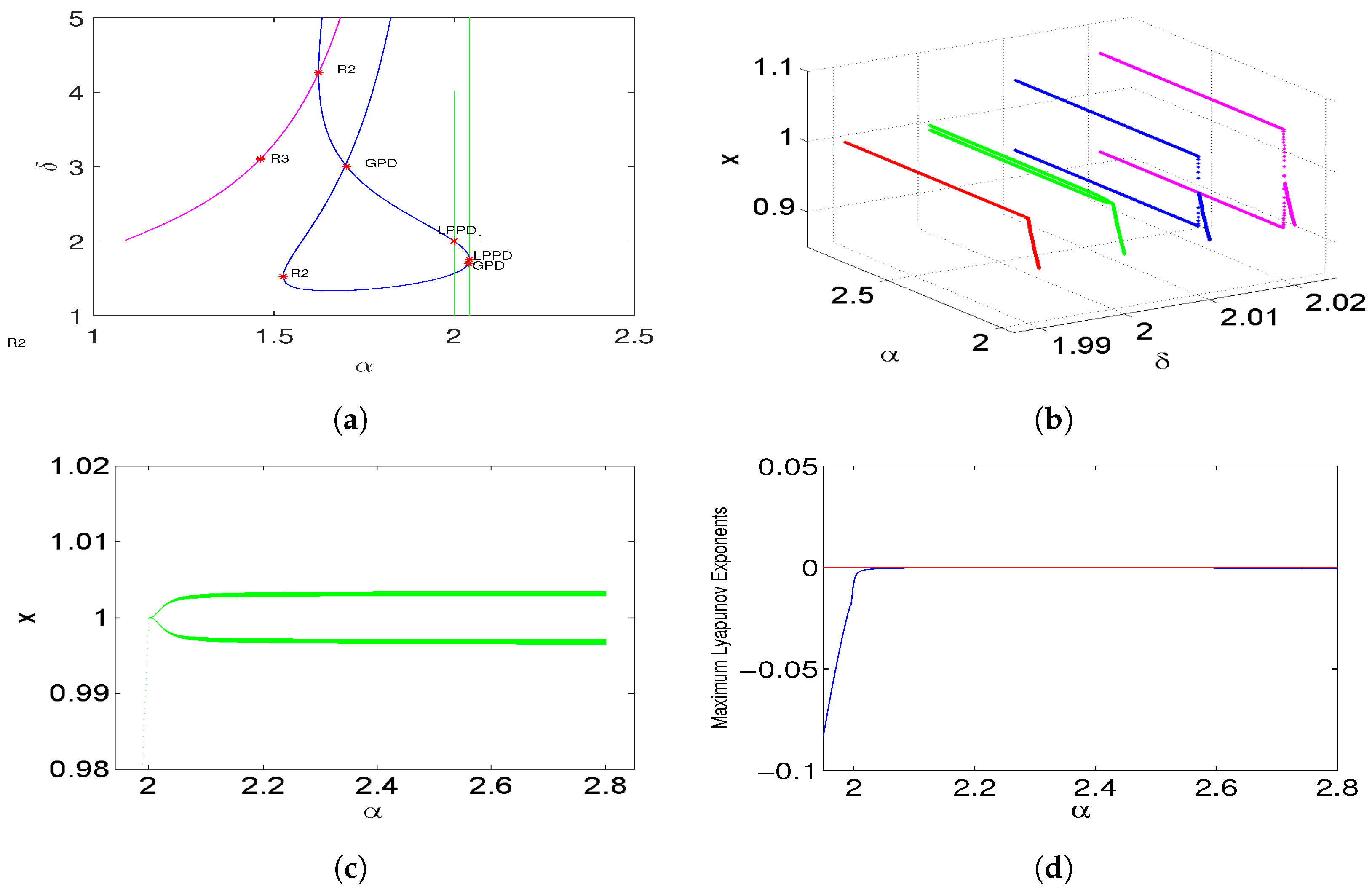
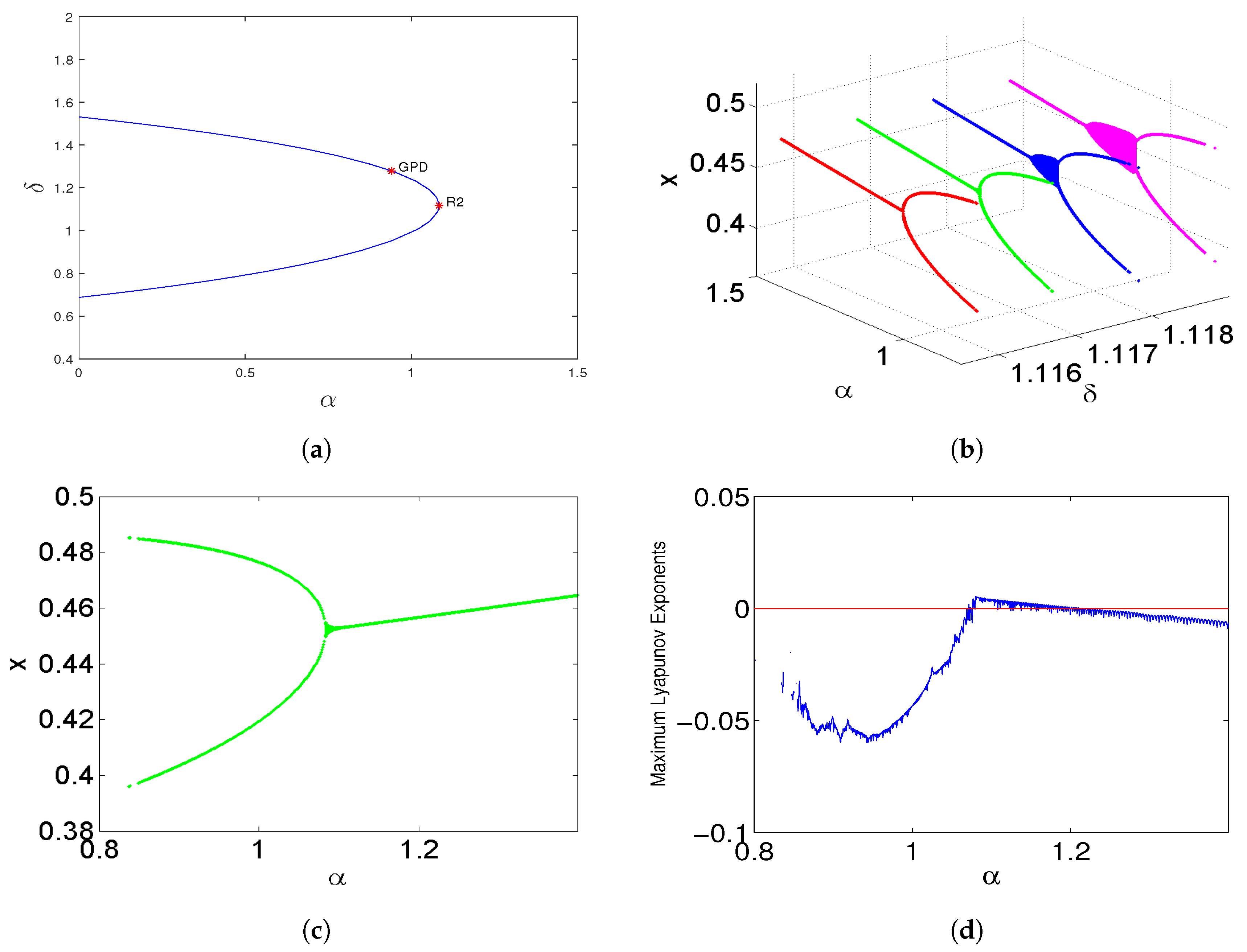
The period doubling continuation curve in the $(\delta ,\alpha )$ plane is shown in Figure 8a. There are two fold–flip bifurcation points, two generalized period doubling points, two 1:2 resonance points, and a 1:3 resonance point. They are marked as LPPD, GPD, R2, and R3, respectively, in Figure 8a. Figure 8b shows a 3-dimensional bifurcation diagram in $(\delta ,\alpha ,x)$ space near $E_0$. Here, δ and α change in a neighborhood of $({\delta }^{*},{\alpha }^{*})=(2,2)$, which is the ${\mathrm{LPPD}}_1$ point in Figure 8a. Figure 8c shows a bifurcation diagram in the $(\alpha ,x)$ plane. Here, $\delta ={\delta }^{*}=2$ and α is the varying parameter. This corresponds to the left bifurcation diagram in Figure 8b. The Lyapunov exponents for the bifurcation diagram in Figure 8c are calculated in Figure 8d.

Figure 8. (a) Continuation curve diagram in the $(\delta ,\alpha ,x)$ plane. The green, blue, and magenta lines represent the LP, PD, and NS continuation curves, respectively. LPPD—fold–flip bifurcation, R2—1:2 resonance, R3—1:3 resonance, GPD—general period double. ${\mathrm{LPPD}}_1$ for $(x,y,\alpha ,\delta )$ is $(1,0,2,2)$. (b) Bifurcation diagram in the $(\delta ,\alpha ,x)$ plane. From left to right, the values of parameter $\delta$ are 1.99, 2, 2.01, and 2.02, respectively. (c) Bifurcation diagram in the $(\delta ,x)$ plane when $\delta ={\delta }^{*}=2$. (d) Maximum Lyapunov exponent corresponding to (c).

Example 7.

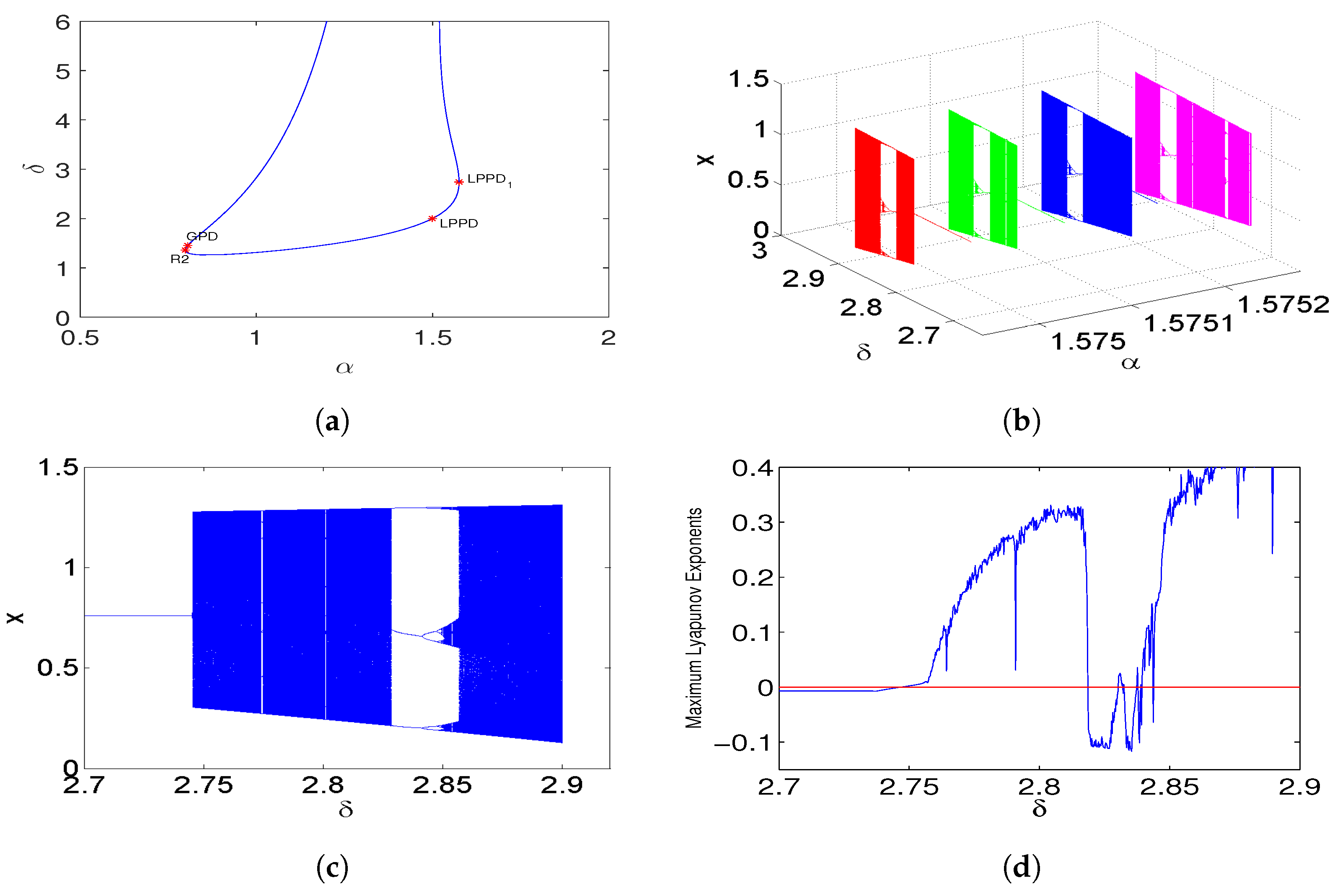
When we fix $\gamma =1.5$, $m=1$, and $\beta =0.3$, we obtain $E_1(0.759544,0.240456)$ and the critical parameter values ${\alpha }^{*}=1.575182$ and ${\delta }^{*}=2.741670$. Moreover, we calculate that ${\lambda }_1=1$, ${\lambda }_2=-1$, $g_{11}=2.808647$, and $\mathrm{Det}\left({\displaystyle \frac{\partial \varphi }{\partial (w,\kappa )}}\right){|}_{w=\kappa =\mathbf{0}}=-2.134977$. According to Theorem 9, map (3) has a fold–flip bifurcation at $E_1$, which is ${\mathrm{LPPD}}_1$ in Figure 9a. Figure 9a shows the PD continuation curve diagram in $(\delta ,\alpha ,x)$ space. Figure 9b is the bifurcation diagram in $(\alpha ,\delta ,x)$ space. Figure 9c is the bifurcation diagram in the $(\delta ,x)$ plane when $\alpha ={\alpha }^{*}=1.57516$. Figure 9d is the maximum Lyapunov exponent corresponding to Figure 9c. Phase portraits for various values of δ corresponding to Figure 9c are given in Figure 10.

Figure 9. (a) PD continuation curve diagram in $(\delta ,\alpha ,x)$ space. The values of $(x,y,\alpha ,\delta )$ at ${\mathrm{LPPD}}_1$ are $(0.759544,0.240456,1.575182,2.741670)$. (b) Bifurcation diagram in $(\delta ,\alpha ,x)$ space. From left to right, the parameter $\delta$ takes the values 1.574982, 1.575082, 1.575182, and 1.575282, respectively. (c) Bifurcation diagram in the $(\alpha ,x)$ plane when $\alpha$ is equal to its value at the critical point, i.e., $\alpha ={\alpha }^{*}=1.575182$. (d) The maximum Lyapunov exponent corresponding to the diagram in (c).

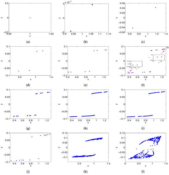
Figure 10. Phase portraits for various values of $\delta$ corresponding to Figure 9c are as follows: (a) Fold–flip bifurcation phase portrait when $\delta =2.74167$. (b) Period-2 phase portrait for $\delta =2.745$. (c) Chaotic behavior for $\delta =2.476$. (d) Chaotic behavior for $\delta =2.477$. (e) Chaotic behavior for $\delta =2.479$. (f) Period-3 phase portrait for $\delta =2.83$. (g) Period-6 phase portrait for $\delta =2.847$. (h) Period-12 phase portrait for $\delta =2.849$.

4.2. 1:2 Resonance

In this subsection, we will consider the 1:2 resonance of map (3) by choosing $\delta$ and $\alpha$ as bifurcation parameters. Based on Theorem 1 (IV)(v) or Theorem 3 (V), if $\delta =2$, $\alpha =(m+1)\gamma$ or $\delta =-{\displaystyle \frac{4}{{\zeta }_{1k}}}$, ${\zeta }_{1k}<0$ and ${\zeta }_{2k}={\displaystyle \frac{{\zeta }_{1k}^2}{4}}$, map (3) exist two critical eigenvalues ${\lambda }_1=-1$, ${\lambda }_2=-1$ at the fixed point $E_0(1,0)$, or $E_k(x_k,y_k)$$(k=1,2,3)$, respectively. Thus a codimension 2 bifurcation associated with 1:2 strong resonance may occur at $E_0$ or $E_k$, respectively. For simplicity, we let $E^{*}(x^{*},y^{*})$ denote the fixed point $E_0(1,0)$ or $E_k(x_k,y_k)$, ${\delta }^{*}$ and ${\alpha }^{*}$ denote critical parameter values.

For convenience, we rewrite the above parameters as $\delta ={\delta }^{*}$ and $\alpha ={\alpha }^{*}$. Further, we denote $\kappa ={(\delta ,\alpha )}^T$, ${\kappa }^{*}={({\delta }^{*},{\alpha }^{*})}^T$.

Let $u_{1,n}=x_n-x^{*}$ and $u_{2,n}=y_n-y^{*}$. Then, we transform $E^{*}(x^{*},y^{*})$ to $O(0,0)$ and expand the right-hand side of system (3)

$$\left(\begin{array}{c}{u}_{1,n+1}\\ u_{2,n+1}\end{array}\right)=\left(\begin{array}{cc}1-\delta c_{11}& -\delta c_{12}\\ \delta c_{21}& 1+\delta c_{22}\end{array}\right)\left(\begin{array}{c}{u}_{1,n}\\ u_{2,n}\end{array}\right)+\left(\begin{array}{c}f\left(u_{1,n},u_{2,n}\right)\\ g\left(u_{1,n},u_{2,n}\right)\end{array}\right)$$

(41)

where

$$\begin{array}{c}{c}_{11}=c_{12}=x^{*},c_{21}={\displaystyle \frac{\beta y^{*2}}{x^{*2}}},c_{22}=-{\displaystyle \frac{\beta y^{*}}{x^{*}}}+{\displaystyle \frac{y^{*}\alpha }{{(\gamma +y^{*})}^2}},f(u_n,v_n)=-\delta u_{1,n}^2-\delta u_{1,n}{u}_{2,n},\hfill \\ g(u_n,v_n)=-{\displaystyle \frac{\beta y^{*2}\delta }{x^{*3}}}{u}_{1,n}^2+{\displaystyle \frac{2\beta \delta y^{*}}{x^{*2}}}{u}_{1,n}{u}_{2,n}+\left({\displaystyle \frac{\delta \alpha }{{(\gamma +y^{*})}^2}}+{\displaystyle \frac{y^{*}\alpha }{{\left(\gamma +y^{*}\right)}^3}}-{\displaystyle \frac{\beta \delta }{x^{*}}}\right)u_{2,n}^2+{\displaystyle \frac{\beta \delta y^{*2}}{x^{*4}}}{u}_{1,n}^3\hfill \\ -{\displaystyle \frac{2\beta \delta y^{*}}{x^{*3}}}{u}_{1,n}^2{u}_{2,n}+{\displaystyle \frac{\beta \delta }{x^{*2}}}{u}_{1,n}{u}_{2,n}^2+\left(-{\displaystyle \frac{\delta \alpha y^{*}}{{(\gamma +y^{*})}^4}}-{\displaystyle \frac{1}{{(\gamma +y^{*})}^3}}\right)u_{2,n}^3+\mathcal{O}\left(\parallel (u_{1,n},u_{2,n}){\parallel }^4\right).\hfill \end{array}$$

(42)

We denote $A\left(\kappa \right)=\left(\begin{array}{cc}1-\delta c_{11}& -\delta c_{12}\\ \delta c_{21}& 1+\delta c_{22}\end{array}\right)$, and $A_1=A\left({\kappa }^{*}\right)$. The eigenvalue of $A_1$ is $-1$. The corresponding eigenvector is $q_2={\left(-\delta c_{12},-2+\delta c_{11}\right)}^T$ and the generalized eigenvector is $q_3={(0,1)}^T$. They satisfy $A_1{q}_2=-q_2$ and $A_1{q}_3=-q_3+q_2$. At the same time, for $A_1^T$ with the eigenvalue $-1$, the eigenvector is and the generalized eigenvector is $p_2={\left({\displaystyle \frac{1}{-\delta c_{12}}},0\right)}^T$. They satisfy $A_1^T{p}_3=-p_3$ and $A_1^T{p}_2=-p_2+p_3$. These four vectors satisfy the following equations:

$$⟨p_2,q_2⟩=⟨p_3,q_3⟩=1,⟨p_2,q_3⟩=⟨p_3,q_2⟩=0,$$

where $⟨.,.⟩$ is the standard scalar product in ${\mathbb{R}}^2$.

Make an invertible linear transformation

$$\left(\begin{array}{c}{u}_{1,n}\\ u_{2,n}\end{array}\right)=v_{1,n}{q}_2+v_{2,n}{q}_3=\left(\begin{array}{cc}-\delta c_{12}& 0\\ -2+\delta c_{11}& 1\end{array}\right)\left(\begin{array}{c}{v}_{1,n}\\ v_{2,n}\end{array}\right).$$

In the coordinates $(v_{1,n},v_{2,n})$, the map has the form:

$$\left(\begin{array}{c}{v}_{1,n+1}\\ v_{2,n+1}\end{array}\right)=\left(\begin{array}{cc}-1& 1\\ d_{10}\left(\kappa \right)& -1+d_{01}\left(\kappa \right)\end{array}\right)\left(\begin{array}{c}{v}_{1,n}\\ v_{2,n}\end{array}\right)+\left(\begin{array}{c}{f}_1(v_{1,n},v_{2,n},\kappa )\\ g_1(v_{1,n},v_{2,n},\kappa )\end{array}\right),$$

(43)

where

$$\begin{array}{c}{f}_1(v_{1,n},v_{2,n})=2\delta v_{1,n}^2-\delta v_{1,n}{v}_{2,n},\hfill \\ g_1(v_{1,n},v_{2,n})=g_{20}{v}_{1,n}^2+g_{11}{v}_{1,n}{v}_{2,n}+g_{02}{v}_{2,n}^2+g_{30}{v}_{1,n}^3+g_{21}{v}_{1,n}^2{v}_{2,n}+g_{12}{v}_{1,n}{v}_{2,n}^2+g_{03}{v}_{2,n}^3+\mathcal{O}(\parallel v_n{\parallel }^4),\hfill \\ d_{10}\left(\kappa \right)=(c_{11}{c}_{22}-c_{12}{c}_{21}){\delta }^2+2(c_{11}-c_{22})\delta -4,d_{01}\left(\kappa \right)=-(c_{11}+c_{22})\delta +4,\hfill \\ g_{20}={\displaystyle \frac{\delta \alpha \gamma {(\delta -2)}^2}{{(y^{*}+\gamma )}^3}}+{\displaystyle \frac{4\delta \beta (y^{*}\delta -1)}{x^{*}}}-\delta (\beta y^{*}{\delta }^2-4+(2x^{*}-4\beta )\delta ),\hfill \\ g_{11}={\displaystyle \frac{2\delta \alpha \gamma (x^{*}\delta -2)}{{(y^{*}+\gamma )}^3}}-{\displaystyle \frac{2\delta \beta (y^{*}\delta -2)}{x^{*}}}+(-2+(x^{*}-2\beta )\delta )\delta ,g_{02}=-{\displaystyle \frac{\beta \delta }{x}}+{\displaystyle \frac{(\alpha \gamma \delta }{{(y^{*}+\gamma )}^3}},\hfill \\ g_{30}=-{\displaystyle \frac{\delta \alpha \gamma {(x^{*}\delta -2)}^3}{{(y^{*}+\gamma )}^4}}-{\displaystyle \frac{{\delta }^2\beta {(y^{*}\delta -2)}^2}{x^{*}}}-{\delta }^3[-4+(1+y^{*})\delta ]\beta ,\hfill \\ g_{21}=-{\displaystyle \frac{3\delta \alpha \gamma {(x^{*}\delta -2)}^2}{{(y^{*}+r)}^4}}-{\displaystyle \frac{2{\delta }^2\beta (y^{*}\delta -2)}{x^{*}}}-2{\delta }^3\beta ,g_{12}=-{\displaystyle \frac{3\delta \alpha \gamma (x^{*}\delta -2)}{{(y^{*}+\gamma )}^4}}-{\displaystyle \frac{{\delta }^2\beta }{x^{*}}},g_{03}=-{\displaystyle \frac{\delta \alpha \gamma }{{(y^{*}+\gamma )}^4}}.\hfill \end{array}$$

If we denote by

$$\left\{\begin{array}{c}{\rho }_1=d_{10}\left(k\right),\hfill \\ {\rho }_2=d_{01}\left(k\right),\hfill \end{array}\right.$$

(44)

then ${\rho }_1\left({\kappa }^{*}\right)={\rho }_2\left({\kappa }^{*}\right)=0$. Map (43) can be rewritten as

$$\left(\begin{array}{c}{v}_{1,n+1}\\ v_{2,n+1}\end{array}\right)=\left(\begin{array}{cc}-1& 1\\ {\rho }_1& -1+{\rho }_2\end{array}\right)\left(\begin{array}{c}{v}_{1,n}\\ v_{2,n}\end{array}\right)+\left(\begin{array}{c}{f}_1(v_{1,n},v_{2,n},\kappa )\\ g_1(v_{1,n},v_{2,n},\kappa )\end{array}\right).$$

(45)

Now we take the following transformation

$$\left\{\begin{array}{c}{v}_{1,n}=w_{1,n}+\sum m_{ij}\left(\rho \right)w_{1,n}^i{w}_{2,n}^j,\hfill \\ v_{2,n}=w_{2,n}+\sum n_{ij}\left(\rho \right)w_{1,n}^i{w}_{2,n}^j.\hfill \end{array}\right.$$

(46)

Fixing $\rho =\mathbf{0}$, to simplify notation, denote $m_{ij}\left(\mathbf{0}\right)=m_{ij}$, $n_{ij}\left(\mathbf{0}\right)=n_{ij}$, $f_{ij}\left(\mathbf{0}\right)=m_{ij}$, $g_{ij}\left(\mathbf{0}\right)=m_{ij}$, where

$$\begin{array}{c}{m}_{20}=\delta +{\displaystyle \frac{g_{20}}{4}},m_{11}={\displaystyle \frac{1}{2}}\delta +{\displaystyle \frac{1}{2}}{g}_{20}+{\displaystyle \frac{1}{4}}{g}_{11},m_{02}={\displaystyle \frac{1}{8}}{g}_{20}+{\displaystyle \frac{1}{4}}{g}_{02}+{\displaystyle \frac{1}{4}}{g}_{11}-{\displaystyle \frac{1}{4}}\delta ,\hfill \\ m_{30}={\displaystyle \frac{1}{12}}{g}_{11}^2+{\displaystyle \frac{1}{24}}(6g_{02}+4g_{20}+6\delta )g_{11}+{\displaystyle \frac{1}{24}}{g}_{20}^2+{\displaystyle \frac{1}{24}}(6g_{02}+2\delta )g_{20}-{\displaystyle \frac{5}{3}}{\delta }^2+{\displaystyle \frac{1}{6}}{g}_{12},\hfill \\ m_{21}=-{\displaystyle \frac{17}{4}}{\delta }^2+{\displaystyle \frac{1}{16}}(4g_{02}+10g_{11}-2g_{20})\delta +{\displaystyle \frac{1}{2}}{g}_{02}^2+{\displaystyle \frac{1}{16}}(18g_{11}+12g_{20})g_{02}+{\displaystyle \frac{3}{8}}{g}_{11}^2+{\displaystyle \frac{9}{16}}{g}_{11}{g}_{20},\hfill \\ +{\displaystyle \frac{1}{8}}{g}_{20}^2+{\displaystyle \frac{1}{2}}{g}_{03}+{\displaystyle \frac{1}{2}}{g}_{12},\hfill \\ m_{12}={\displaystyle \frac{7}{24}}{g}_{11}^2+{\displaystyle \frac{1}{48}}(42g_{02}+19g_{20}+6\delta )g_{11}+{\displaystyle \frac{1}{12}}{g}_{20}^2+{\displaystyle \frac{1}{48}}(24g_{02}-16\delta )g_{20}+{\displaystyle \frac{1}{2}}{g}_{02}^2-{\displaystyle \frac{7}{3}}{\delta }^2+{\displaystyle \frac{1}{2}}{g}_{03}+{\displaystyle \frac{1}{3}}{g}_{12},\hfill \\ n_{20}={\displaystyle \frac{g_{20}}{2}},n_{11}={\displaystyle \frac{g_{20}}{2}}+{\displaystyle \frac{g_{11}}{2}},n_{02}={\displaystyle \frac{g_{11}}{4}}+{\displaystyle \frac{g_{02}}{2}},n_{30}=-{\displaystyle \frac{1}{2}}\delta (8\delta +g_{20}),n_{03}\left(\rho \right)=m_{03}\left(\rho \right)=0,\hfill \\ n_{21}={\displaystyle \frac{1}{4}}{g}_{11}^2+{\displaystyle \frac{1}{8}}(6g_{02}+4g_{20}+2\delta )g_{11}+{\displaystyle \frac{1}{8}}{g}_{20}^2+{\displaystyle \frac{1}{8}}(6g_{02}-8\delta )g_{20}-6{\delta }^2+{\displaystyle \frac{1}{2}}{g}_{12},\hfill \\ n_{12}={\displaystyle \frac{1}{8}}{g}_{20}^2+{\displaystyle \frac{1}{8}}(6g_{02}+5g_{11}-4\delta )g_{20}+g_{02}^2+{\displaystyle \frac{3}{2}}{g}_{02}{g}_{11}+{\displaystyle \frac{1}{2}}{g}_{11}^2-2{\delta }^2+g_{03}+{\displaystyle \frac{1}{2}}{g}_{12}.\hfill \end{array}$$

The normal form of 1:2 resonance for map (45) can be obtained as

$$\left(\begin{array}{c}{w}_{1,n+1}\\ w_{2,n+1}\end{array}\right)=\left(\begin{array}{cc}-1& 1\\ {\rho }_1& -1+{\rho }_2\end{array}\right)\left(\begin{array}{c}{w}_{1,n}\\ w_{2,n}\end{array}\right)+\left(\begin{array}{c}0\\ C\left(\rho \right)w_{1,n}^3+D\left(\rho \right)w_{1,n}^2{w}_{2,n}+\mathcal{O}\left(\parallel (w_{1,n},w_{2,n}){\parallel }^4\right)\end{array}\right),$$

(47)

in which

$$\begin{array}{c}C\left(\rho \right)=\left[{\displaystyle \frac{1}{24}}{g}_{20}^2+{\displaystyle \frac{1}{12}}(3g_{02}+2g_{11}+\delta )g_{20}+{\displaystyle \frac{1}{4}}{g}_{11}{g}_{02}+{\displaystyle \frac{1}{12}}{g}_{11}^2+{\displaystyle \frac{1}{4}}{g}_{11}\delta -{\displaystyle \frac{5}{3}}{\delta }^2+{\displaystyle \frac{1}{6}}{g}_{12}\right]{\rho }_1+\left(-{\displaystyle \frac{1}{2}}\delta g_{20}-4{\delta }^2\right){\rho }_2\hfill \\ +{\displaystyle \frac{1}{2}}{g}_{20}^2+{\displaystyle \frac{1}{2}}(4\delta +g_{11})g_{20}+g_{30},\hfill \\ D\left(\rho \right)=\left[{\displaystyle \frac{1}{8}}{g}_{20}^2+{\displaystyle \frac{1}{16}}(12g_{02}+9g_{11}-2\delta )g_{20}+{\displaystyle \frac{3}{8}}{g}_{11}^2+{\displaystyle \frac{1}{8}}(9g_{02}+5\delta )g_{11}+{\displaystyle \frac{1}{2}}{g}_{02}^2+{\displaystyle \frac{1}{4}}\delta g_{02}-{\displaystyle \frac{17}{4}}{\delta }^2+{\displaystyle \frac{1}{2}}{g}_{03}\right.\hfill \\ \left.+{\displaystyle \frac{1}{2}}{g}_{12}\right]{\rho }_1+\left[{\displaystyle \frac{1}{8}}{g}_{20}^2+{\displaystyle \frac{1}{4}}(2g_{11}-4\delta +3g_{02})g_{20}+{\displaystyle \frac{1}{4}}{g}_{11}^2+{\displaystyle \frac{1}{4}}(\delta +3g_{02})g_{11}-6{\delta }^2+{\displaystyle \frac{1}{2}}{g}_{12}\right]{\rho }_2\hfill \\ +g_{20}^2+{\displaystyle \frac{1}{4}}\left(5g_{11}+10\delta +4g_{02}\right)g_{20}+{\displaystyle \frac{1}{2}}{g}_{11}^2+g_{11}\delta +12{\delta }^2+g_{21}.\hfill \end{array}$$

Represent the normal form map (47) as

$$w\mapsto {\Phi }_{\rho }\left(w\right).$$

Then, we will make an approximation of this map by means of a flow. When $\rho =\mathbf{0}$,

$$\left(\begin{array}{c}{w}_{1,n}\\ w_{2,n}\end{array}\right)\mapsto \left(\begin{array}{cc}-1& 1\\ 0& -1\end{array}\right)\left(\begin{array}{c}{w}_{1,n}\\ w_{2,n}\end{array}\right)$$

has negative eigenvalues, so the map ${\Phi }_{\rho }$ cannot be approximated by a flow. Nevertheless, the second iteration ${\Phi }_{\rho }^2$ can be approximated by the unit-time shift of a flow. The form of the map ${\Phi }_{\rho }^2$ is as

$$\left(\begin{array}{c}{w}_1\\ w_2\end{array}\right)\mapsto \left(\begin{array}{cc}-1+{\rho }_1& -2+{\rho }_2\\ -2{\rho }_1+{\rho }_1{\rho }_2& 1+{\rho }_1-2{\rho }_2+{\rho }_2^2\end{array}\right)\left(\begin{array}{c}{w}_1\\ w_2\end{array}\right)+\left(\begin{array}{c}F(w,\rho )\\ G(w,\rho )\end{array}\right),$$

(48)

where $F(w,\rho )=C\left(\rho \right)w_1^3+D\left(\rho \right)w_1^2{w}_2$, $G(w,\rho )=(-2C\left(\rho \right)+{\rho }_{1}D\left(\rho \right)+{\rho }_{2}C\left(\rho \right))w_1^3+(3C\left(\rho \right)-2D\left(\rho \right)-2{\rho }_{1}D\left(\rho \right)+{\rho }_{2}D\left(\rho \right))w_1^2{w}_2+$$(-3C\left(\rho \right)+2D\left(\rho \right)+{\rho }_{1}D\left(\rho \right)-2{\rho }_{2}D\left(\rho \right))w_1{w}_2^2+(C\left(\rho \right)-D\left(\rho \right)+{\rho }_{2}D\left(\rho \right))w_2^3+{\mathcal{O}(\parallel w\parallel }^4)$.

When $\parallel \rho \parallel$ is sufficiently small, map (48) is close to the identity map and can be approximated by a flow according to [40]. Due to that,

$${\displaystyle e^{{\Psi }_{\rho }}=I+{\Sigma }_{k=1}\frac{1}{k!}{\Psi }_{\rho }^k=\left(\begin{array}{cc}1+{\rho }_1& -2+{\rho }_2\\ -2{\rho }_1+{\rho }_1{\rho }_2& 1+{\rho }_1-2{\rho }_2+{\rho }_2^2\end{array}\right),}$$

(49)

where

$${\Psi }_{\rho }^k\left(\begin{array}{cc}1+{\rho }_1& -2-{\displaystyle \frac{2}{3}}{\rho }_1-{\rho }_2\\ -2{\rho }_1+{\rho }_1{\rho }_2& -{\rho }_1-2{\rho }_2\end{array}\right)+{\mathcal{O}(\parallel \rho \parallel }^2),$$

(50)

and there is no quadratic term in map (48).

We assume that the approximating cubic system has the form

$$\begin{array}{c}\left(\begin{array}{c}{\dot{w}}_1\\ {\dot{w}}_2\end{array}\right)=\Psi \left(\begin{array}{c}{w}_1\\ w_2\end{array}\right)+\left(\begin{array}{c}{F}_{30}\left(\rho \right)w_1^3+F_{21}\left(\rho \right)w_1^2{w}_2+F_{12}\left(\rho \right)w_1{w}_2^2+F_{03}\left(\rho \right)w_2^3\\ G_{30}\left(\rho \right)w_1^3+G_{21}\left(\rho \right)w_1^2{w}_2+G_{12}\left(\rho \right)w_1{w}_2^2+G_{03}\left(\rho \right)w_2^3\end{array}\right)+{\mathcal{O}(\parallel w\parallel }^4)\hfill \\ =\Psi \left(\begin{array}{c}{w}_1\\ w_2\end{array}\right)+H_{\rho }(w_1,w_2)+{\mathcal{O}(\parallel w\parallel }^4),\hfill \end{array}$$

(51)

where $F_{ij}\left(\rho \right)$ and $G_{ij}\left(\rho \right)$ with $i+j=3$ are unknown coefficients that need to be defined. For the sake of simplified notation, we let $F_{ij}\left(\rho \right)=F_{ij}$ and $G_{ij}\left(\rho \right)=G_{ij}$, which will be provided later. Now, let us carry out three Picard iterations for system (51). Since the system (51) has no quadratic terms, we obtain

$$\begin{array}{c}{\left(\begin{array}{c}{w}_1\\ w_2\end{array}\right)}^{\left(1\right)}\left(\theta \right)={\left(\begin{array}{c}{w}_1\\ w_2\end{array}\right)}^{\left(2\right)}\left(\theta \right)=e^{{\Psi }_{\rho }\theta }\left(\begin{array}{c}{w}_1\\ w_2\end{array}\right)\hfill \\ =\left(\begin{array}{cc}1-\theta {\rho }_1+2{\theta }^2{\rho }_1+{\mathcal{O}(\parallel \rho \parallel }^2)& -\theta (2+{\displaystyle \frac{3}{2}}{\rho }_1+{\rho }_2)+2{\theta }^2({\rho }_1+{\rho }_2)+{\mathcal{O}(\parallel \rho \parallel }^2)\\ -2{\rho }_1\theta +{\mathcal{O}(\parallel \rho \parallel }^2)& 1-\theta ({\rho }_1+2{\rho }_2)+2{\theta }^2{\rho }_1+{\mathcal{O}(\parallel \rho \parallel }^2)\end{array}\right).\hfill \end{array}$$

(52)

The third iteration yields

$$\begin{array}{c}{\displaystyle {\left(\begin{array}{c}{w}_1\\ w_2\end{array}\right)}^{\left(3\right)}\left(\theta \right)=e^{{\Psi }_{\rho }\theta }\left(\begin{array}{c}{w}_1\\ w_2\end{array}\right)+{\int }_0^{\theta }{e}^{{\Psi }_{\rho }(\theta -t)}H\left(w_1^{\left(2\right)},w_2^{\left(2\right)}\right)\mathrm{d}t.}\hfill \end{array}$$

(53)

Letting $\theta =1$, we obtain

$$\begin{array}{c}{\left(\begin{array}{c}{w}_1\\ w_2\end{array}\right)}^{\left(3\right)}\left(1\right)\hfill \\ =\left(\begin{array}{c}(1+{\rho }_1)w_1+(-2+{\rho }_2)w_2+r_{30}{w}_1^3+r_{21}{w}_1^2{w}_2+r_{12}{w}_1{w}_2^2+r_{03}{w}_2^3+\mathcal{O}\left(\parallel (w_1,w_2){\parallel }^4\right)\\ (-2{\rho }_1+{\rho }_1{\rho }_2)w_1+(1+{\rho }_1-2{\rho }_2+{\rho }^2)w_2+s_{30}{w}_1^3+s_{21}{w}_1^2{w}_2+s_{12}{w}_1{w}_2^2+s_{03}{w}_2^3+\mathcal{O}\left(\parallel (w_1,w_2){\parallel }^4\right)\end{array}\right),\hfill \end{array}$$

(54)

where

$$\begin{array}{c}{r}_{30}=F_{30}-G_{30},r_{21}=-3F_{30}-F_{21}+2G_{30}-G_{21},r_{12}=4F_{30}-2F_{21}+F_{12}-2G_{30}+{\displaystyle \frac{4}{3}}{G}_{21}-G_{12},\hfill \\ r_{03}=-2F_{30}+{\displaystyle \frac{4}{3}}{F}_{21}-F_{12}+F_{03}+{\displaystyle \frac{4}{5}}{G}_{30}-{\displaystyle \frac{2}{3}}(G_{21}-G_{12})-G_{03},s_{30}=G_{30},s_{21}=-3G_{30}+G_{21},\hfill \\ s_{12}=4G_{30}-2G_{21}+G_{12},s_{03}=-2G_{30}+{\displaystyle \frac{4}{3}}{G}_{21}-G_{12}+G_{03}.\hfill \end{array}$$

Based on Equations (48), (51) and (54), we obtain

$$\begin{array}{c}{F}_{30}=-C\left(\rho \right),F_{21}=-2C\left(\rho \right)-D\left(\rho \right),F_{12}=-C\left(\rho \right)-{\displaystyle \frac{4}{3}}D\left(\rho \right),F_{03}=-{\displaystyle \frac{1}{15}}C\left(\rho \right)-{\displaystyle \frac{4}{3}}D\left(\rho \right),\hfill \\ G_{30}=-2C\left(\rho \right),G_{21}=-3C\left(\rho \right)-2D\left(\rho \right),G_{12}=-C\left(\rho \right)-2D\left(\rho \right),G_{03}=-{\displaystyle \frac{1}{3}}D\left(\rho \right).\hfill \end{array}$$

Then, we obtain ${\Psi }_{\rho }^2={\psi }_{\rho }^1+\mathcal{O}\left(\parallel (w_1,w_2){\parallel }^4\right)$, where ${\psi }_{\rho }^1$ represents the flow of the system (51) and can be further simplified.

Let

$$\left\{\begin{array}{c}{v}_1=w_1+\left({\displaystyle \frac{1}{6}}{F}_{12}\left(\rho \right)+{\displaystyle \frac{1}{12}}{G}_{12}\left(\rho \right)\right)w_1^3+\left({\displaystyle \frac{1}{4}}{F}_{12}\left(\rho \right)+{\displaystyle \frac{1}{4}}{G}_{03}\left(\rho \right)\right)w_1^2{w}_2+{\displaystyle \frac{1}{2}}{F}_{03}\left(\rho \right)w_1{w}_2^2,\hfill \\ v_2=-{\rho }_1{w}_1-\left(2+{\displaystyle \frac{2}{3}}{\rho }_1+{\rho }_2\right)w_2+F_{30}\left(\rho \right)w_1^3-{\displaystyle \frac{1}{2}}{G}_{12}\left(\rho \right)w_1^2{w}_2-G_{03}{w}_1{w}_2^2.\hfill \end{array}\right.$$

Then, we can obtain

$$\begin{array}{c}\left(\begin{array}{c}{\dot{v}}_1\\ {\dot{v}}_2\end{array}\right)=\left(\begin{array}{cc}0& 1\\ 4{\rho }_1+{\mathcal{O}(\parallel \rho \parallel }^2)& -2{\rho }_1-2{\rho }_2+{\mathcal{O}(\parallel \rho \parallel }^2)\end{array}\right)\left(\begin{array}{c}{v}_1\\ v_2\end{array}\right)+\left(\begin{array}{c}0\\ C_1\left(\rho \right)v_1^3+D_1\left(\rho \right)v_1^2{v}_2\end{array}\right),\hfill \end{array}$$

(55)

in which

$$\begin{array}{c}{C}_1\left(\rho \right)=\left[-3\delta g_{11}-13\delta g_{20}-{\displaystyle \frac{31}{6}}{g}_{20}{g}_{11}+g_{02}{g}_{11}-3g_{20}{g}_{02}-4g_{21}-{\displaystyle \frac{5}{3}}{g}_{30}-{\displaystyle \frac{14}{3}}{g}_{20}^2-{\displaystyle \frac{5}{3}}{g}_{11}^2-{\displaystyle \frac{164}{3}}{\delta }^2+{\displaystyle \frac{2}{3}}{g}_{12}\right]{\rho }_1\hfill \\ +\left(-16{\delta }^2+2\delta g_{20}+g_{11}{g}_{20}+g_{20}^2+2g_{30}\right){\rho }_2+8\delta g_{20}+2g_{20}{g}_{11}+2g_{20}^2+4g_{30},\hfill \\ D_1\left(\rho \right)=\left[-{\displaystyle \frac{1}{2}}\delta g_{02}-g_{02}^2-g_{03}-{\displaystyle \frac{13}{12}}\delta g_{11}+{\displaystyle \frac{89}{12}}\delta g_{20}+{\displaystyle \frac{5}{6}}{g}_{20}{g}_{11}-{\displaystyle \frac{15}{4}}{g}_{02}{g}_{11}-{\displaystyle \frac{4}{3}}{g}_{20}{g}_{02}+{\displaystyle \frac{5}{3}}{g}_{21}+{\displaystyle \frac{7}{4}}{g}_{30}+{\displaystyle \frac{49}{24}}{g}_{20}^2\right.\hfill \\ \left.-{\displaystyle \frac{5}{12}}{g}_{11}^2+{\displaystyle \frac{77}{2}}{\delta }^2-2g_{12}\right]{\rho }_1+\left[-{\displaystyle \frac{3}{2}}{g}_{02}{g}_{11}-{\displaystyle \frac{1}{2}}{g}_{20}{g}_{02}+{\displaystyle \frac{1}{2}}\delta g_{11}-g_{12}+g_{21}+{\displaystyle \frac{1}{2}}{g}_{20}{g}_{11}+{\displaystyle \frac{17}{2}}\delta g_{20}+g_{20}^2\right.\hfill \\ \left.+48{\delta }^2+{\displaystyle \frac{1}{2}}{g}_{30}\right]{\rho }_2-2g_{20}{g}_{02}-{\displaystyle \frac{11}{2}}{g}_{20}{g}_{11}-2g_{21}-6g_{30}-2\delta g_{11}-17\delta g_{20}-24{\delta }^2-g_{11}^2-5g_{20}^2.\hfill \end{array}$$

According to Theorem 9.3 in [40], the unit-time flow of system (51) can be used to approximate ${\Psi }_{\rho }^2$. Next, we will consider the bifurcations of the approximating system (51).

We make the assumption that non-degeneracy conditions

$$C_1\left(0\right)\ne 0,D_1\left(0\right)\ne 0.$$

(56)

Suppose that $D_1\left(0\right)<0$ (otherwise, reverse time). Based on the result of the 1:2 resonance in [40], we conclude that system (3) has a 1:2 resonance at $E^{*}$ at $\kappa ={\kappa }^{*}$ under condition (52), and the bifurcation behavior of system (3) can be approximated by system (51). In order to scale the variables, parameters, and time in system (51), we introduce

$$x_1={\displaystyle \frac{-D_1\left(\rho \right)}{\sqrt{\pm C_1\left(\rho \right)}}}{v}_1,x_2={\displaystyle \frac{D_1^2\left(\rho \right)}{C_1\left(\rho \right)\sqrt{\pm C_1\left(\rho \right)}}}{v}_2,t={\displaystyle \frac{-C_1\left(\rho \right)}{D_1\left(\rho \right)}}\tau .$$

(57)

where we use “+” if $C_1\left(0\right)>0$ and “−” if $C_1\left(0\right)<0$.

Under this transformation, system (51) can be written as

$$\left\{\begin{array}{c}{\displaystyle \frac{\mathrm{d}{x}_1}{\mathrm{d}t}}=x_2,\hfill \\ {\displaystyle \frac{\mathrm{d}{x}_2}{\mathrm{d}t}}={ϵ}_1{x}_1+{ϵ}_2{x}_2\pm x_1^3-x_1^2{x}_2,\hfill \end{array}\right.$$

(58)

where “+” for $C_1\left(0\right)>0$, “−” for $C_1\left(0\right)<0$, and

$${ϵ}_1=(4{\rho }_1+{\mathcal{O}(\parallel \rho \parallel }^2\left)\right){\displaystyle \frac{D_1^2\left(\rho \right)}{C_1^2\left(\rho \right)}},{ϵ}_2=2({\rho }_1+{\rho }_2+{\mathcal{O}(\parallel \rho \parallel }^2\left)\right){\displaystyle \frac{D_1\left(\rho \right)}{C_1\left(\rho \right)}}.$$

(59)

Due to that

$$\mathrm{Det}\left({\displaystyle \frac{\partial ϵ}{\partial \rho }}\right){|}_{\rho =\mathbf{0}}={\displaystyle \frac{8D_1^3\left(\rho \right)}{C_1^3\left(\rho \right)}}\ne 0,$$

and therefore Equation (54) is locally invertible. We can solve ${\rho }_1$ and ${\rho }_2$ from Equation (59) as follows

$$\left\{\begin{array}{c}{\rho }_1={\displaystyle \frac{C_1^2\left(0\right)}{4D_1^2\left(0\right)}}{ϵ}_1+{\mathcal{O}(\parallel ϵ\parallel }^2),\hfill \\ {\rho }_2=-{\displaystyle \frac{C_1^2\left(0\right)}{4D_1^2\left(0\right)}}{ϵ}_1+{\displaystyle \frac{C_1\left(0\right)}{2D_1\left(0\right)}}{ϵ}_2+{\mathcal{O}(\parallel ϵ\parallel }^2).\hfill \end{array}\right.$$

(60)

Using the result from [40], we enumerate the possible bifurcation behaviors of the approximating system (53) in the vicinity of the origin.

(i)

There is a pitchfork bifurcation curve

$$F=\left\{({ϵ}_1,{ϵ}_2)\right|{ϵ}_1=0\};$$

(61)

(ii)

There is a non-degenerate Hopf bifurcation curve

$$H=\left\{({ϵ}_1,{ϵ}_2)\right|{ϵ}_2=0,{ϵ}_1<0\};$$

(62)

(iii)

There is a heteroclinic Hopf bifurcation curve

$$CH=\left\{({ϵ}_1,{ϵ}_2)\right|{ϵ}_2=-{\displaystyle \frac{1}{5}}{ϵ}_1+\mathcal{O}\left({ϵ}_1\right),{ϵ}_1<0\}.$$

(63)

Theorem 10.

If the conditions $\delta =2$$\alpha =(m+1)\gamma$ or $\delta =-{\displaystyle \frac{4}{{\zeta }_{1k}}}$, ${\zeta }_{2k}={\displaystyle \frac{{\zeta }_{1k}^2}{4}}$, and ${\zeta }_{1k}<0$ are satisfied, and also $C_1\left(0\right)\ne 0$ and $D_1\left(0\right)\ne 0$, then system (3) has a 1:2 strong resonance at $E^{*}$. Moreover, near $E^{*}$, the system has these bifurcation behaviors:

(i)

there is a flip bifurcation curve like the pitchfork bifurcation curve in (61). Crossing this curve makes a stable period-2 cycle come from $E^{*}$.

(ii)

there is a non-degenerate Neimark–Sacker bifurcation curve like in (62). Crossing it leads to a stable closed invariant cycle around $E^{*}$.

(iii)

there is a homoclinic structure. This means there are long-period cycles that appear and disappear through fold bifurcations in a very narrow parameter region around $CH$ in (63).

Example 8.

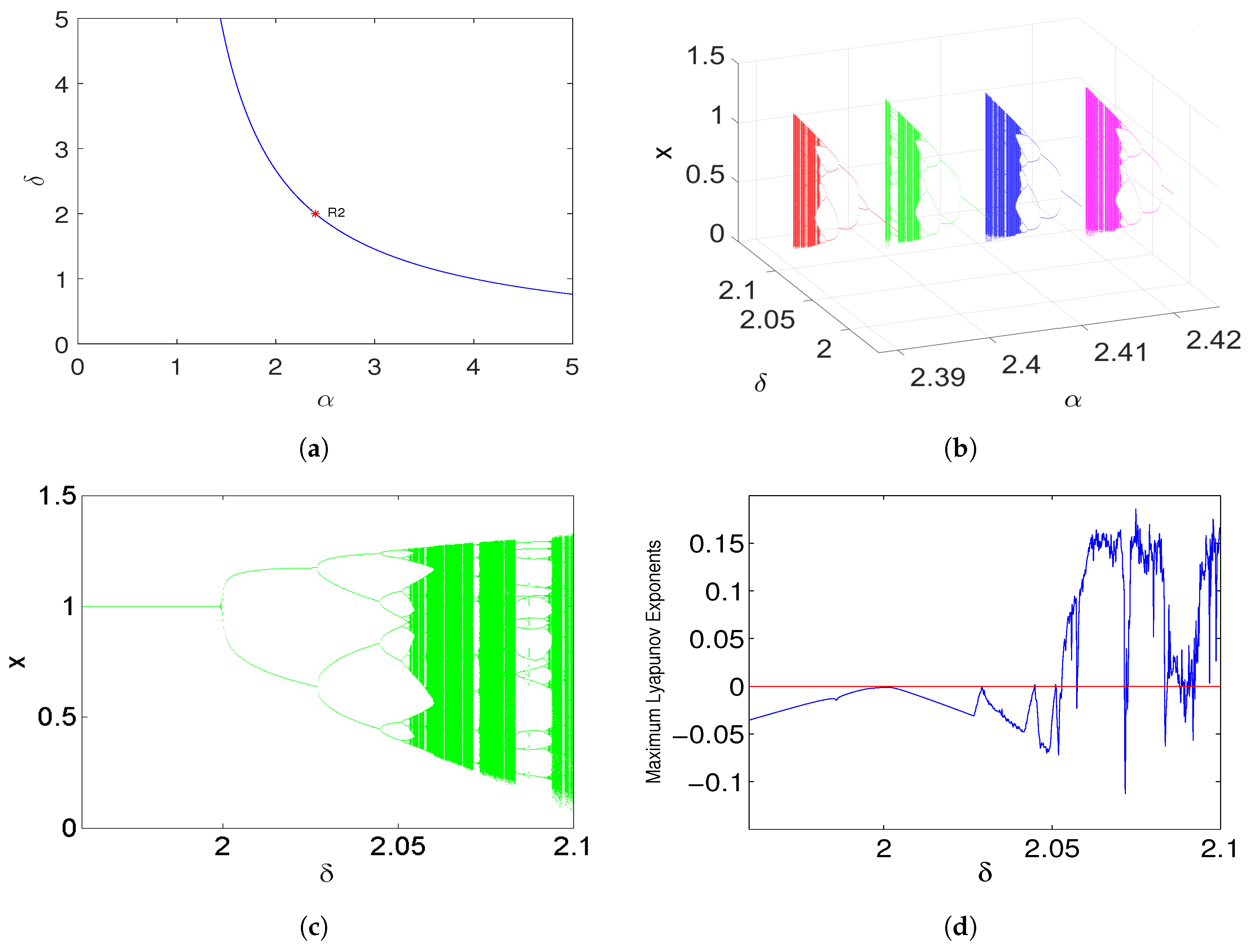
For $E_0(1,0)$, set $\gamma =1.6$, $m=0.5$, and $\beta =0.8$. Then, we have ${\alpha }^{*}=2.4$ and ${\delta }^{*}=2$. Also, ${\lambda }_1={\lambda }_2=-1$, $C_1\left(0\right)=46.080000\ne 0$, and $D_1\left(0\right)=122.720000$. From Theorem 10, system (3) has a 1:2 strong resonance at $E_0(1,0)$ (that is R2 in Figure 11a).

Figure 11. (a) PD continuation curve diagram in the $(\alpha ,\delta )$ plane. For $(x,y,\alpha ,\delta )$, the value of R2 is $(1,0,2.4,2)$. (b) Bifurcation diagram in $(\delta ,\alpha ,x)$ space. The parameter $\alpha$ takes the values 2.39, 2.40, 2.41, and 2.42 from left to right, respectively. (c) Bifurcation diagram in the $(\delta ,x)$ plane when $\alpha ={\alpha }^{*}=2.4$. (d) The maximum Lyapunov exponent corresponding to (c).

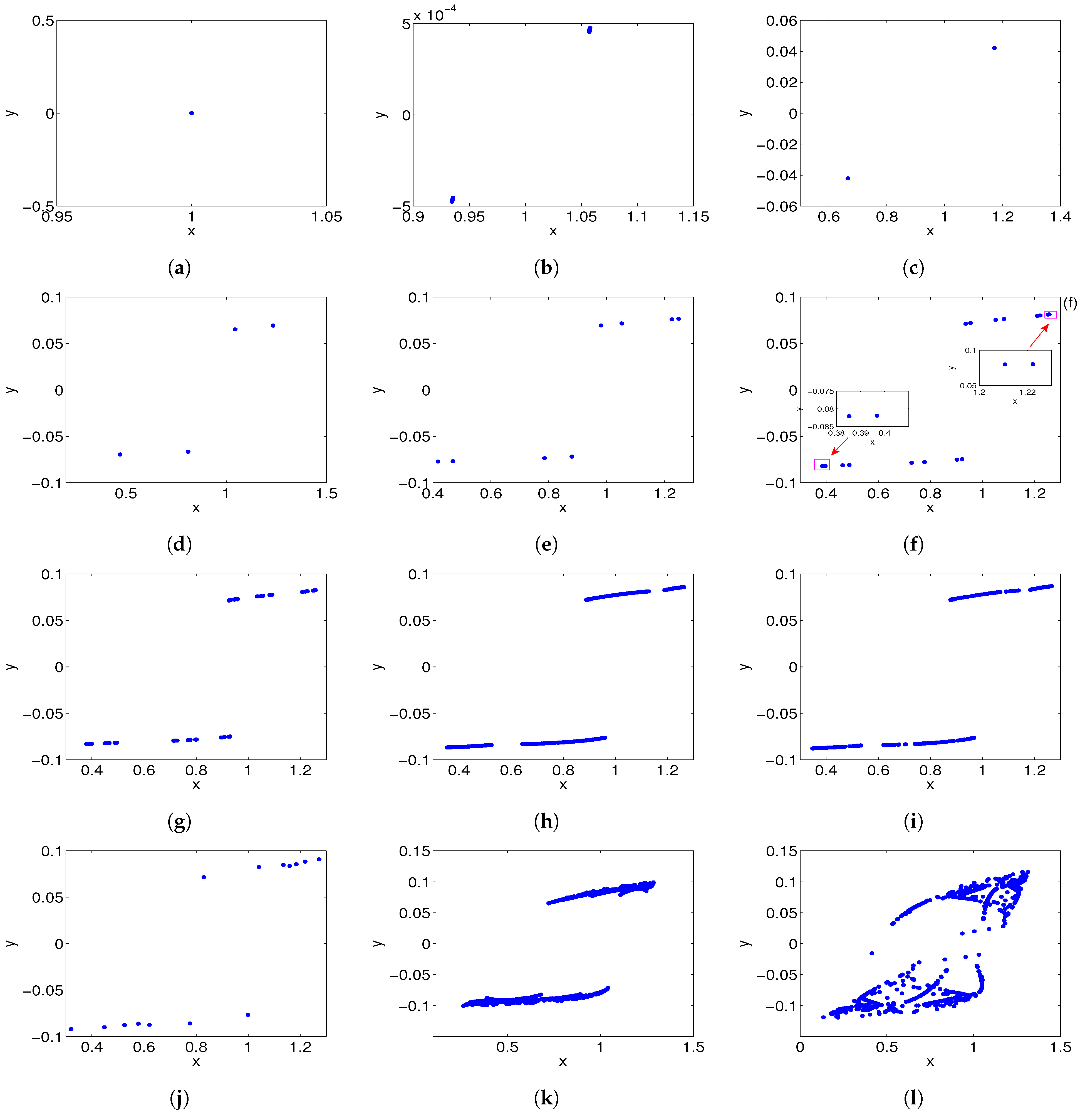
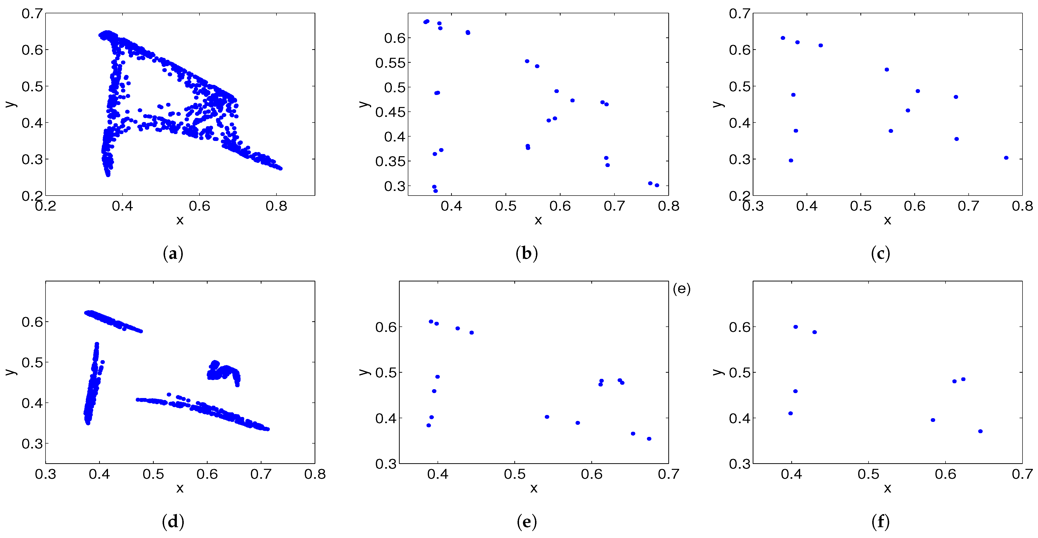
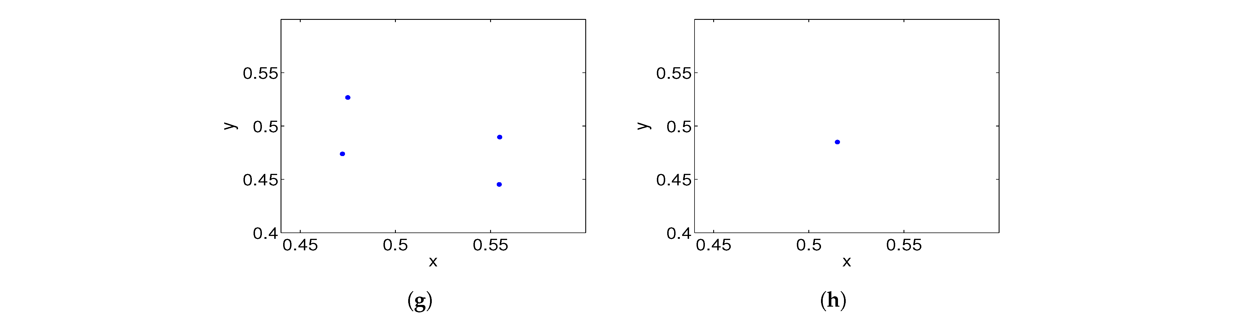
The continuation of the PD curve for the two control parameters δ and α is plotted in Figure 11a. A 1:2 strong resonance (R2) is found. Figure 11b shows a 3D bifurcation diagram in $(\delta ,\alpha ,x)$ space near $E^{*}$ when δ and α change near $({\delta }^{*},{\alpha }^{*})=(2,2.4)$ (the R2 point in Figure 11a). Figure 11c is a 2D bifurcation diagram in the $(\delta ,x)$ plane when $\alpha ={\alpha }^{*}=2.4$ and δ changes from 0 to 2.1. Figure 11d has the maximum Lyapunov exponents for Figure 11c. Some of these exponents are negative and some are positive, which means system (3) has chaotic behavior near the 1:2 strong resonance point $E^{*}$. Figure 12a–l show the phase portraits of system (3) near $E^{*}$ with different δ and α values.

Figure 12. The phases corresponding to Figure 11c are as follows: (a) when $\delta =1.99$; (b) the 1:2 resonance phase at $\delta =2$; (c) the phase portrait of period-3 at $\delta =2.02$; (d) the phase portrait of period-4 at $\delta =2.04$; (e) the phase portrait of period-8 at $\delta =2.047$; (f) the phase portrait of period-16 at $\delta =2.052$; (g) the phase portrait of period-48 at $\delta =2.053$; (h) chaotic behavior at $\delta =2.057$; (i) chaotic behavior at $\delta =2.058$; (j) the phase portrait of period-14 at $\delta =2.063$; (k) chaotic behavior at $\delta =2.07$; (l) chaotic behavior at $\delta =2.094$.

Example 9.

Fixing $\gamma =1.5$, $m=3.8$, $\beta =2.7$, we have $E_2(0.452192,0.547808)$ and ${\alpha }^{*}=1.083465$, ${\delta }^{*}=1.116828$. Then, $C_1\left(0\right)=40.319888\ne 0$, $D_1\left(0\right)=146.440431$. According to Theorem 10, system (3) has a 1:2 strong resonance at $E_2$, which is R2 as shown in Figure 13a.

Figure 13. (a) Continuation curve diagram in the $(\alpha ,\delta )$ plane. The magenta line shows the NS continuation curve. For $(x,y,\alpha ,\delta )$, the value of R2 is $(0.452192,0.547808,1.083465,1.116828)$. (b) Bifurcation diagram in $(\delta ,\alpha ,x)$ space. The values of the parameter $\delta$ from left to right are 1.115828, 1.116828, 1.117828, and 1.118828. (c) 1:2 strong resonance bifurcation diagram in the $(\alpha ,x)$ plane when $\delta ={\delta }^{*}=1.116828$. (d) The maximum Lyapunov exponent corresponding to (c).

Figure 13a is PD continuation curve diagram in the $(\alpha ,\delta )$ plane. The 1:2 strong reasonance point R2, which will be showed in Figure 13b, and a GPD point are detected. Figure 13b is bifurcation diagram in the $(\delta ,\alpha ,x)$ plane. From left to right, $\delta =1.11583,1.11683,1.11783,$$1.11883$. Figure 13c is bifurcation diagram in the $(\alpha ,x)$ plane when $\delta ={\delta }^{*}=1.116828$. Figure 13d is the maximum Lyapunov exponent corresponding to Figure 13c.

4.3. 1:4 Strong Resonance

In this subsection, we will consider the 1:4 resonance of map (3) by selecting two parameters, $\delta$ and $\alpha$, as bifurcation parameters. Based on Theorem 3 (VI), if $\delta =-{\displaystyle \frac{2}{{\zeta }_{1k}}}$, ${\zeta }_{1k}<0$, and ${\zeta }_{2k}={\displaystyle \frac{{\zeta }_{1k}^2}{2}}$, map (3) has two critical eigenvalues ${\lambda }_1=\mathrm{i}$, ${\lambda }_2=-\mathrm{i}$ at the fixed point $E_k(x_k,y_k)$$(k=1,2,3)$. Thus, a codimension 2 bifurcation associated with the 1:4 strong resonance may occur at $E_k$. For simplicity, we let $E^{*}(x^{*},y^{*})$$(k=1,2,3)$ denote the fixed point $E_k(x_k,y_k)$, and ${\delta }^{*}$ and ${\alpha }^{*}$ denote critical parameter values.

Similar to Section 4.2, by translating $E_k$$(k=1,2,3)$ into $O(0,0)$ and expanding the right side of the map into a Taylor series, we can obtain

$$\left(\begin{array}{c}{u}_{1,n+1}\\ u_{2,n+1}\end{array}\right)=\left(\begin{array}{cc}1+\delta c_{11}& \delta c_{12}\\ \delta c_{21}& 1+\delta c_{22}\end{array}\right)\left(\begin{array}{c}{u}_{1,n}\\ u_{2,n}\end{array}\right)+\left(\begin{array}{c}\delta F_1\left(u_{1,n},u_{2,n}\right)\\ \delta F_2\left(u_{1,n},u_{2,n}\right)\end{array}\right),$$

(64)

where all the letters mean the same as Equation (42). The Jacobian matrix at $E^{*}$ is $J\left(ϵ\right)=\left(\begin{array}{cc}1+\delta d_{11}& \delta d_{12}\\ \delta d_{21}& 1+\delta d_{22}\end{array}\right)$. We set $A_1=A\left({ϵ}_{*}\right)$, then $A_1{q}_4={\lambda }_1{q}_4$, $A_1^T{p}_4={\overline{\lambda }}_1{p}_4$, where ${\lambda }_1=\mathrm{i}$, $q_4={\left(q_{41},q_{42}\right)}^T={(\delta c_{12},-1-\delta c_{11}+\mathrm{i})}^T$, $p_4={\left(p_{41},p_{42}\right)}^T={\left({\displaystyle \frac{-1+(1+\delta c_{11})\mathrm{i}}{2\delta c_{12}}},{\displaystyle \frac{\mathrm{i}}{2}}\right)}^T$ and $⟨p_4,q_4⟩=1$, where $⟨.,.⟩$ represents the standard scalar product in ${\mathbb{R}}^2$.

Let $U={(u_1,u_2)}^T=z{q}_4+\overline{z}{\overline{q}}_4\in {\mathbb{R}}^2$. Map (64) can be written in the complex form as follow:

$$\begin{array}{c}{\displaystyle z(n+1)={\lambda }_{1}z\left(n\right)+\sum _{2\le i+j\le 3}{\alpha }_{i,j}{z}^i\left(n\right){\overline{z}}^j\left(n\right)+\mathcal{O}\left(\parallel (z\left(n\right),\overline{z}\left(n\right)){\parallel }^4\right),}\hfill \end{array}$$

(65)

where ${\lambda }_1=\mathrm{i}$ and

$$\begin{array}{c}{\alpha }_{20}=(f_{11}{q}_{41}{q}_{42}+f_{20}{q}_{41}^2){\overline{p}}_{41}+(g_{02}{q}_{42}^2+g_{11}{q}_{41}{q}_{42}+g_{20}{q}_{41}^2){\overline{p}}_{42},\hfill \\ {\alpha }_{11}=(f_{11}{q}_{41}{\overline{q}}_{42}+f_{11}{\overline{q}}_{41}{q}_{42}+2f_{20}{q}_{41}{\overline{q}}_{41}){\overline{p}}_{41}+(2g_{02}{q}_{42}{\overline{q}}_{42}+g_{11}{q}_{41}{\overline{q}}_{42}+g_{11}{\overline{q}}_{41}{q}_{42}+2g_{20}{q}_{41}{\overline{q}}_{41}){\overline{p}}_{42},\hfill \\ {\alpha }_{02}=(f_{11}{\overline{q}}_{41}{\overline{q}}_{42}+f_{20}{\overline{q}}_{41}^2){\overline{p}}_{41}+(g_{02}{\overline{q}}_{42}^2+g_{11}{\overline{q}}_{41}{\overline{q}}_{42}+g_{20}{\overline{q}}_{41}^2){\overline{p}}_{42},\hfill \\ {\alpha }_{30}={\overline{p}}_{42}(g_{03}{q}_{42}^3+g_{12}{q}_{41}{q}_{42}^2+g_{21}{q}_{41}^2{q}_{42}+g_{30}{q}_{41}^3),\hfill \\ {\alpha }_{21}=(3{\overline{p}}_{42}{g}_{03}{\overline{q}}_{42}+{\overline{p}}_{42}{g}_{12}{\overline{q}}_{41})q_{42}^2+2{\overline{p}}_{42}{q}_{42}(g_{12}{\overline{q}}_{42}+g_{21}{\overline{q}}_{41})q_{41}+{\overline{p}}_{42}(g_{21}{\overline{q}}_{42}+3g_{30}{\overline{q}}_{41})q_{41}^2,\hfill \\ {\alpha }_{12}=(3{\overline{p}}_{42}{g}_{03}{q}_{42}+{\overline{p}}_{42}{g}_{12}{q}_{41}){\overline{q}}_{42}^2+2{\overline{p}}_{42}{\overline{q}}_{42}(g_{12}{q}_{42}+g_{21}{q}_{41}){\overline{q}}_{41}+{\overline{p}}_{42}(g_{21}{q}_{42}+3g_{30}{q}_{41}){\overline{q}}_{41}^2,\hfill \\ {\alpha }_{03}={\overline{p}}_{42}(g_{03}{\overline{q}}_{42}^3+g_{12}{\overline{q}}_{41}{\overline{q}}_{42}^2+g_{21}{\overline{q}}_{41}^2{\overline{q}}_{42}+g_{30}{q}_{41}^3).\hfill \end{array}$$

(66)

and ${\overline{\alpha }}_{ij}$ is the complex conjugate of ${\alpha }_{ij}$.

To establish the normal form for 1:4 strong resonance, we will get rid of some quadratic terms in map (65) with the transformation

$$z\left(n\right)=\phi \left(n\right)+{\displaystyle \frac{{\beta }_{20}}{2}}{\phi }^2\left(n\right)+{\beta }_{11}\phi \left(n\right)\overline{\phi }\left(n\right)+{\displaystyle \frac{{\beta }_{02}}{2}}{\overline{\phi }}^2\left(n\right),$$

(67)

and its inverse transformation

$$\begin{array}{c}\phi \left(n\right)=z\left(n\right)-{\displaystyle \frac{{\beta }_{20}}{2}}{z}^2\left(n\right)+{\beta }_{11}z\left(n\right)\overline{z}\left(n\right)+{\displaystyle \frac{{\beta }_{02}}{2}}{\overline{z}}^2\left(n\right)+{\displaystyle \frac{1}{2}}\left({\beta }_{20}^2+{\beta }_{11}{\overline{\beta }}_{02}\right)z^3\left(n\right)+\left(|{\beta }_{11}{|}^2+{\displaystyle \frac{3}{2}}{\beta }_{11}{\beta }_{20}\right.\hfill \\ \left.+{\displaystyle \frac{1}{2}}{\left|{\beta }_{11}\right|}^2\right)z^2\left(n\right)\overline{z}\left(n\right)+\left({\beta }_{02}\left|{\beta }_{11}\right|+{\beta }_{11}^2+{\displaystyle \frac{1}{2}}{\beta }_{11}{\overline{\beta }}_{20}+{\displaystyle \frac{1}{2}}{\beta }_{20}{\beta }_{02}\right)z\left(n\right){\overline{z}}^2\left(n\right)\hfill \\ +{\displaystyle \frac{1}{2}}\left({\beta }_{11}{\beta }_{02}+{\beta }_{02}{\overline{\beta }}_{20}\right){\overline{z}}^3\left(n\right)+\mathcal{O}\left(\parallel (z\left(n\right),\overline{z}\left(n\right)){\parallel }^4\right).\hfill \end{array}$$

(68)

Combining map (67) and (68), we will transform map (65) into the following form

$$\begin{array}{c}\phi (n+1)={\lambda }_1ϵ\left(n\right)+\sum _{2\le i+j\le 3}{\gamma }_{i,j}{\phi }^i\left(n\right){\overline{\phi }}^j\left(n\right)+\mathcal{O}\left(\parallel (\phi \left(n\right),\overline{\phi }\left(n\right)){\parallel }^4\right),\hfill \end{array}$$

(69)

where

$$\begin{array}{c}{\gamma }_{20}={\displaystyle \frac{1+\mathrm{i}}{2}}{\beta }_{20}+{\alpha }_{20},{\gamma }_{11}=(-1+\mathrm{i}){\beta }_{11}+{\alpha }_{11},{\gamma }_{02}={\displaystyle \frac{1+\mathrm{i}}{2}}{\beta }_{02}+{\alpha }_{02},\hfill \\ {\gamma }_{30}={\displaystyle \frac{1-\mathrm{i}}{2}}{\beta }_{20}^2+(1-\mathrm{i}){\alpha }_{20}{\beta }_{20}-{\displaystyle \frac{1+\mathrm{i}}{2}}{\beta }_{11}{\overline{\beta }}_{02}+{\displaystyle \frac{1}{2}}{\alpha }_{11}{\overline{\beta }}_{02}+\mathrm{i}{\beta }_{11}{\overline{\alpha }}_{02}+{\alpha }_{30},\hfill \\ {\gamma }_{21}={\displaystyle \frac{1+3\mathrm{i}}{2}}{\beta }_{20}{\beta }_{11}+(2+\mathrm{i}){\alpha }_{20}{\beta }_{11}-\mathrm{i}{\overline{\alpha }}_{11}{\beta }_{11}+{\displaystyle \frac{1-2\mathrm{i}}{2}}{\alpha }_{11}{\beta }_{20}+{\overline{\beta }}_{11}{\alpha }_{11}+{\displaystyle \frac{1}{2}}{\alpha }_{02}{\overline{\beta }}_{02}\hfill \\ +\mathrm{i}{\overline{\alpha }}_{02}{\beta }_{02}+{\displaystyle \frac{\mathrm{i}+1}{2}}|{\beta }_{02}{|}^2+(\mathrm{i}-1){\left|{\beta }_{11}\right|}^2+{\alpha }_{21},\hfill \\ {\gamma }_{12}=(-1-\mathrm{i}){\beta }_{11}^2-{\displaystyle \frac{1+\mathrm{i}}{2}}{\overline{\beta }}_{20}{\beta }_{11}+(1+\mathrm{i}){\alpha }_{11}{\beta }_{11}-\mathrm{i}{\overline{\alpha }}_{20}{\beta }_{11}+(1-\mathrm{i}){\overline{\beta }}_{11}{\beta }_{02}+\mathrm{i}{\overline{\alpha }}_{11}{\beta }_{02}\hfill \\ +2{\alpha }_{20}{\beta }_{02}+{\displaystyle \frac{1-\mathrm{i}}{2}}{\beta }_{20}{\beta }_{02}-\mathrm{i}{\beta }_{20}{\alpha }_{02}+2{\overline{\beta }}_{11}{\alpha }_{02}+{\displaystyle \frac{1}{2}}{\overline{\beta }}_{20}{\alpha }_{11}+{\alpha }_{12},\hfill \\ {\gamma }_{03}={\displaystyle \frac{1+\mathrm{i}}{2}}{\overline{\beta }}_{20}{\beta }_{02}+{\displaystyle \frac{\mathrm{i}-1}{2}}{\beta }_{11}{\beta }_{02}+\mathrm{i}{\overline{\alpha }}_{20}{\beta }_{02}+{\displaystyle \frac{1}{2}}{\alpha }_{11}{\beta }_{02}+\mathrm{i}{\beta }_{11}{\alpha }_{02}+{\overline{\beta }}_{20}{\alpha }_{02}+{\alpha }_{03}.\hfill \end{array}$$

We choose

$$\begin{array}{c}{\beta }_{20}=-{\displaystyle \frac{2{\alpha }_{20}}{1+\mathrm{i}}},{\beta }_{11}={\displaystyle \frac{{\alpha }_{11}}{1-\mathrm{i}}},{\beta }_{02}=-{\displaystyle \frac{2{\alpha }_{02}}{1+\mathrm{i}}},\hfill \end{array}$$

(70)

Then, map (69) becomes

$$\begin{array}{c}\phi (n+1)={\lambda }_1\phi \left(n\right)+\sum _{i+j=3}{\gamma }_{i,j}{\phi }^i\left(n\right){\overline{\phi }}^j\left(n\right)+\mathcal{O}\left(\parallel (\phi \left(n\right),\overline{\phi }\left(n\right)){\parallel }^4\right).\hfill \end{array}$$

(71)

Next, with the intention of eliminating the cubic terms, we employ a transformation

$$\phi \left(n\right)=\varphi \left(n\right)+{\displaystyle \frac{{\beta }_{30}}{6}}{\varphi }^3\left(n\right)+{\displaystyle \frac{{\beta }_{21}}{2}}\varphi \left(n\right)\overline{\varphi }\left(n\right)+{\displaystyle \frac{{\beta }_{03}}{6}}{\overline{\varphi }}^3\left(n\right),$$

(72)

The inverse transformation of map (72) can be obtained

$$\begin{array}{c}\varphi \left(n\right)=\phi \left(n\right)-{\displaystyle \frac{{\beta }_{30}}{6}}{\phi }^3\left(n\right)-{\displaystyle \frac{{\beta }_{21}}{2}}\phi \left(n\right)\overline{\phi }\left(n\right)-{\displaystyle \frac{{\beta }_{03}}{6}}{\overline{\phi }}^3\left(n\right)+\mathcal{O}\left(\parallel (\phi \left(n\right),\overline{\phi }\left(n\right)){\parallel }^4\right).\hfill \end{array}$$

(73)

By map (72) and (73), map (71) can be transformed into the following form:

$$\begin{array}{c}\varphi (n+1)={\lambda }_1\varphi \left(n\right)+{\displaystyle \sum _{i+j=3}}{\xi }_{i,j}{\varphi }^i\left(n\right){\overline{\varphi }}^j\left(n\right)+\mathcal{O}\left(\parallel (\varphi \left(n\right),\overline{\varphi }\left(n\right)){\parallel }^4\right),\hfill \end{array}$$

(74)

in which

$$\begin{array}{c}{\xi }_{30}={\gamma }_{30}+{\displaystyle \frac{\mathrm{i}}{3}}{\beta }_{30},{\xi }_{21}={\gamma }_{21},{\xi }_{12}={\gamma }_{12}+\mathrm{i}{\beta }_{12},{\xi }_{03}={\gamma }_{03}.\hfill \end{array}$$

Then, map (74) can be reduced into the following form:

$$\begin{array}{c}\varphi (n+1)={\lambda }_1\varphi \left(n\right)+{\alpha }_{02}{\overline{\varphi }}^2\left(n\right)+{\xi }_{21}{\varphi }^2\left(n\right)\overline{\varphi }\left(n\right)+{\xi }_{03}{\overline{\varphi }}^3\left(n\right)+\mathcal{O}\left(\parallel (\varphi \left(n\right),\overline{\varphi }\left(n\right)){\parallel }^4\right)\hfill \end{array}$$

(75)

by taking ${\beta }_{30}=3\mathrm{i}{\gamma }_{30}$, ${\beta }_{21}=0$, ${\beta }_{12}=\mathrm{i}{\gamma }_{12}$, ${\alpha }_{03}=0$.

Defining

$$\begin{array}{c}{\zeta }_1\left(ϵ\right)=-2\mathrm{i}{\xi }_{21},{\zeta }_2\left(ϵ\right)=-{\displaystyle \frac{2\mathrm{i}}{3}}{\xi }_{03}.\hfill \end{array}$$

(76)

If ${\zeta }_2\left(ϵ\right)\ne 0$, letting ${\zeta }_3={\displaystyle \frac{{\zeta }_1}{|{\zeta }_2|}}$, from [40], we can obtain the following theorem.

Theorem 11.

If $\delta =-{\displaystyle \frac{2}{{\zeta }_{1k}}}$, ${\zeta }_{1k}<0$, ${\zeta }_{2k}={\displaystyle \frac{{\zeta }_{1k}^2}{2}}$, and conditions ${\zeta }_2\ne 0$, $\mathrm{Re}\left({\zeta }_3\right)\ne 0$, $\mathrm{Im}\left({\zeta }_3\right)\ne 0$ hold, system (3) undergoes the 1:4 strong resonance bifurcation at $E_2^{*}$.

Example 10.

Fixing $\gamma =2$, $m=1.2$, $\beta =0.3$, at the fixed point $E^{*}(0.516874,0.483126)$, we have ${\lambda }_{1,2}=\pm \mathrm{i}$, ${\zeta }_1=14324.50649-245.1345104\mathrm{i}$, ${\zeta }_2=-6.680239467+2.204687653\mathrm{i}$ and ${\zeta }_3=8.968040994-0.1534696040\mathrm{i}$. Then, ${\zeta }_2\ne 0$, $\mathrm{Re}\left({\zeta }_3\right)\ne 0$ and $\mathrm{Im}\left({\zeta }_3\right)\ne 0$. According to Theorem 11, system (3) has a 1:4 strong resonance bifurcation at $E^{*}$.

Figure 14a exhibits the continuation curve diagram in the $(\alpha ,\delta )$ plane. In Figure 14a, R4, which is shown in Figure 14b, is detected. Figure 14b is a bifurcation diagram in the $(\delta ,\alpha ,x)$ plane. From left to right, the values of parameter δ are 3.214272, 3.234272, 3.254272, 3.274272, respectively. Figure 14c is a bifurcation diagram in the $(\alpha ,x)$ plane when $\delta ={\delta }^{*}=3.234272$. Figure 14d is the maximum Lyapunov exponent corresponding to Figure 14c. Figure 15 is the phase corresponding to Figure 14c.

Figure 14. (a) Continuation curve diagram in the $(\alpha ,\delta )$ plane. The magenta line represents the NS continuation curve. R4 for $(x,y,\alpha ,\delta )$ is $(0.516874,0.483126,2.283431,3.234272)$. (b) Bifurcation diagram in the $(\delta ,\alpha ,x)$ plane. From left to right, the values of parameter $\delta$ are 3.214272, 3.234272, 3.254272, 3.274272, respectively. (c) 1:4 strong resonance bifurcation diagram in the $(\alpha ,x)$ plane with $\delta ={\delta }^{*}=3.234272$. (d) Maximum Lyapunov exponent corresponding to (c).

Figure 15. The phase corresponding to Figure 14c is as follows: (a) Chaos occurs when $\alpha =2.18$. (b) The phase portrait is of period-26 when $\alpha =2.183$. (c) The phase portrait is of period-13 when $\alpha =2.187$. (d) Chaos occurs when $\alpha =2.2$. (e) The phase portrait is of period-16 when $\alpha =2.21$. (f) The phase portrait is of period-8 when $\alpha =2.22$. (g) The phase portrait is of period-4 when $\alpha =2.27$. (h) There is a stable fixed point when $\alpha =2.28$.

5. Two-Parameter Plane Plots

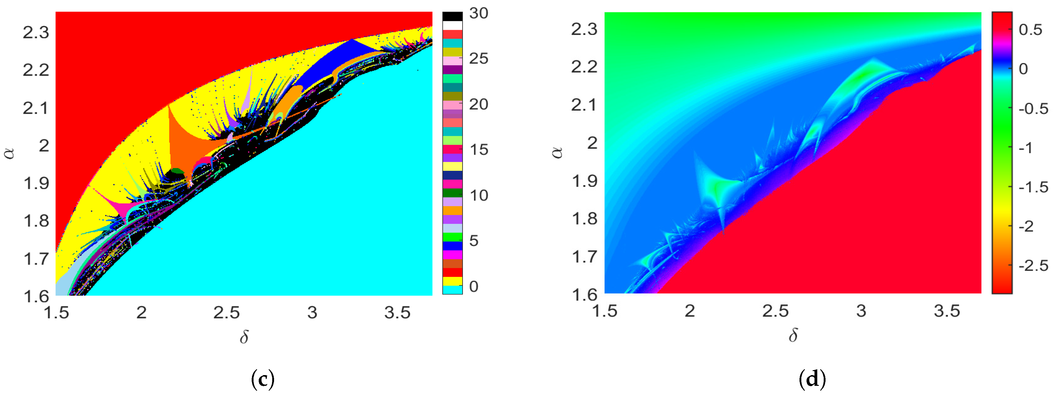
In this section, we look into some two-parameter planes for system (3) by using the method described in [42]. We pick two cases (1:2 strong resonance and 1:4 strong resonance) from the bifurcation scenarios mentioned above for further discussion. When discussing 1:2 strong resonance, we put the one-parameter sequence into the $(\delta ,\alpha )$ parameter plane. Figure 16a,b shows a group of global views in different two-parameter planes, and the fixed parameter values are the same as in Example 8. Figure 16c,d is similar to Figure 16a,b, but it is about the 1:4 strong resonance in Example 9. All the results are obtained by dividing the parameter interval into a grid with $800\times 800$ equally spaced points. For each point in the two-parameter planes on the left of Figure 16, an orbit can go to a quasi-periodic, a periodic attractor, a chaotic state, or an attractor at infinity (divergence). These are shown by the numbers on the colorbar. The cyanine area is for divergence (the number is $-1$), and the black area is for chaos (the number is 30). The colors on the right of Figure 16 are related to the values of the maximum Lyapunov exponents, and red means the area where the maximum Lyapunov exponents diverge (the number is 1). The two-parameter plane plots show the complex dynamic behaviors of the discrete system (3) when the integral step size $\delta$ and other parameters are changed.

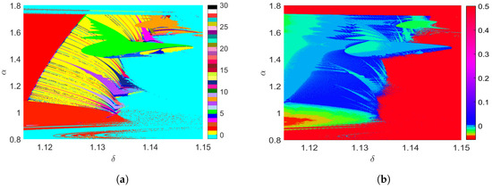
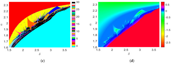
Figure 16. (a) Some two-parameter planes for system (3). The left panel shows a global view of different parameter planes. The numbers represent periods, and the cyanine area is the divergence region (marked with $-1$). The right panel shows the Lyapunov phase diagrams of the parameter planes, where the numbers show the magnitude of the largest Lyapunov exponent. (a,b) are the global views for the 1:2 strong resonance. (c,d) are the global views for the 1:4 strong resonance.

6. Conclusions

In this paper, we studied the complex behaviors of the predator–prey system (3) as a discrete-time system. We mainly analyzed codimension 1 and codimension 2 bifurcations. There are four types in codimension 1 bifurcations: transcritical, fold, flip, and Neimark–Sacker. And there are three types in codimension 2 bifurcations: fold–flip, 1:2, and 1:4 strong resonances. We found that the discretized step size $\delta$ greatly affects the stability of the fixed points of the model.

Compared with the continuous-time model Equation (2) investigated in [24], more detailed theoretical proofs and numerical simulations of phase portraits, single-parameter bifurcations, two-parameter bifurcations, maximum Lyapunov exponents, and two-parameter plane plots are employed to reveal the dynamics of the discrete-time model Equation (3). These not only demonstrate the stability of fixed points but also reveal richer codimension 1 and codimension 2 bifurcation structures. Specifically speaking, the fold–flip bifurcation and resonance bifurcations occurring at the fixed point $E_k$ imply that the discrete system may undergo complex codimension 2 bifurcations near $E_k$. Also, system (3) has some interesting behaviors, like orbits of period-7, -14, -21, invariant cycles, flip bifurcation cascades in period-2, -4, -8 orbits, and chaotic sets. This means the predator–prey system is not stable when there is chaos. Especially, if the prey is in chaos, the predator will either die out or move towards a stable fixed point in the end. The continuous-time model cannot display all the dynamics of low-dimensional predator–prey models, such as chaos. Through the theoretical analysis and numerical simulations provided in this paper, we have observed a rich dynamic behavior that was not observed in the original continuous case proposed in [24]. These complex dynamical behaviors could be useful for understanding the dynamics of the low dimension predator–prey system. This shows that the discrete-time dynamical model has a more significant research value.

In this paper, we mainly study the dynamics of the model discretized by the forward Euler’s method. Using other discretization methods, such as the fourth-order Runge–Kutta method, the explicit midpoint method and so on, the dynamics of the model are worth considering for future research.

References

- Bazykin, A.D. Structural and Dynamic Stability of Model Predator-Prey Systems; International Institute for Applied Systems Analysis: London, UK, 1976. [Google Scholar]
- Reynolds-Hogland, M.J.; Hogland, J.S.; Mitchell, M.S. Evaluating intercepts from demographic models to understand resource limitation and resource thresholds. Ecol. Model. 2008, 211, 424–432. [Google Scholar] [CrossRef]
- Qin, W.J.; Tang, S.Y.; Cheke, R.A. The effects of resource limitation on a predator-prey model with control measures as nonlinear pulses. Math. Probl. Eng. 2014, 2014, 99–114. [Google Scholar] [CrossRef]
- Real, L.A. The kinetics of functional response. Am. Nat. 1977, 111, 289–300. [Google Scholar] [CrossRef]
- Xu, R.; Chaplain, M.A.J.; Davidson, F.A. Periodic solutions for a predator-prey model with Holling-type functional response and time delays. Appl. Math. Comput. 2005, 161, 637–654. [Google Scholar] [CrossRef]
- Ma, Z.; Wang, S. A delay-induced predator-prey model with Holling type functional response and habitat complexity. Nonlinear Dynam. 2018, 93, 1519–1544. [Google Scholar] [CrossRef]
- Xie, Y.; Wang, Z.; Meng, B.; Huang, X. Dynamical analysis for a fractional-order prey-predator model with Holling III type functional response and discontinuous harvest. Appl. Math. Lett. 2020, 106, 106342. [Google Scholar] [CrossRef]
- Hu, D.P.; Li, Y.Y.; Liu, M.; Bai, Y.Z. Stability and Hopf bifurcation for a delayed predator-prey model with stage structure for prey and Ivlev-type functional response. Nonlinear Dynam. 2020, 99, 3323–3350. [Google Scholar] [CrossRef]
- Wang, X.Y.; Zanette, L.; Zou, X.F. Modelling the fear effect in predator-prey interactions. J. Math. Biol. 2016, 73, 1179–1204. [Google Scholar] [CrossRef]
- Panday, P.; Samanta, S.; Pal, N.; Chattopadhyay, J. Delay induced multiple stability switch and chaos in a predator-prey model with fear effect. Math. Comput. Simulat. 2020, 172, 134–158. [Google Scholar] [CrossRef]
- Sarkar, K.; Khajanchi, S. Impact of fear effect on the growth of prey in a predator-prey interaction model. Ecol. Complex. 2020, 42, 100826. [Google Scholar] [CrossRef]
- Martin, A.; Ruan, S.G. Predator-prey models with delay and prey harvesting. J. Math. Biol. 2001, 43, 247–267. [Google Scholar] [CrossRef] [PubMed]
- Liu, M.; Meng, F.W.; Hu, D.P. Impacts of multiple time delays on a gene regulatory network mediated by small noncoding RNA. Int. J. Bifurc. Chaos 2020, 30, 2050069. [Google Scholar] [CrossRef]
- Ruan, S.G. On nonlinear dynamics of predator-prey models with discrete delay. Math. Model. Nat. Phenom. 2009, 4, 140–188. [Google Scholar] [CrossRef]
- Xu, R.; Gan, Q.T.; Ma, Z.E. Stability and bifurcation analysis on a ratio-dependent predator-prey model with time delay. J. Comput. Appl. Math. 2009, 230, 187–203. [Google Scholar] [CrossRef]
- Garain, K.; Mandal, P.S. Bubbling and hydra effect in a population system with Allee effect. Ecol. Complex. 2021, 47, 100939. [Google Scholar] [CrossRef]
- Liu, W.; Jiang, Y.L. Bifurcation of a delayed Gause predator-prey model with Michaelis-Menten type harvesting. J. Theor. Biol. 2018, 438, 116–132. [Google Scholar] [CrossRef] [PubMed]
- May, R.M.; Beddington, J.R.; Clark, C.W.; Holt, S.J.; Laws, R.M. Management of multispecies fisheries. Science 1979, 205, 267–277. [Google Scholar] [CrossRef]
- Xiao, D.M.; Jennings, L.S. Bifurcations of a ratio-dependent predator-prey system with constant rate harvesting. SIAM J. Appl. Math. 2005, 65, 737–753. [Google Scholar] [CrossRef]
- Baek, H. Spatiotemporal dynamics of a predator-prey system with linear harvesting rate. Math. Probl. Eng. 2014, 2014, 625973. [Google Scholar] [CrossRef]
- Wang, Y.; Zhou, X.; Jiang, W.H. Bifurcations in a diffusive predator-prey system with linear harvesting. Chaos Soliton. Fract. 2023, 169, 113286. [Google Scholar] [CrossRef]
- Clark, C.W.; Mangel, M. Aggregation and fishery dynamics: A theoretical study of schooling and the Purse Seine tuna fisheries. Fish. Bull. 1979, 77, 317–337. [Google Scholar]
- Gupta, R.P.; Chandra, P. Bifurcation analysis of modified Leslie-Gower predator-prey model with Michaelis-Menten type prey harvesting. J. Math. Anal. Appl. 2013, 398, 278–295. [Google Scholar] [CrossRef]
- Hu, D.P.; Cao, H.J. Stability and bifurcation analysis in a predator-prey system with Michaelis-Menten type predator harvesting. Nonlinear Anal. Real World Appl. 2017, 33, 58–82. [Google Scholar] [CrossRef]
- Atabaigi, A. Multiple bifurcations and dynamics of a discrete-time predator-prey system withgroup defense and non-monotonic functional response. Differ. Equat. Dyn. Sys. 2020, 28, 107–132. [Google Scholar] [CrossRef]
- Gupta, R.P.; Chandra, P.; Banerjee, M. Dynamical complexity of a prey-predator model with nonlinear predator harvesting. Discret. Cont. Dyn. Sys. B 2015, 20, 423–443. [Google Scholar] [CrossRef]
- Khan, M.S.; Abbas, M.; Bonyah, E.; Qi, H.X. Michaelis-Menten-Type prey harvesting in discrete modified Leslie-Gower predator-prey model. J. Funct. Space 2022, 2022, 1–23. [Google Scholar] [CrossRef]
- Cheng, L.F.; Cao, H.J. Bifurcation analysis of a discrete-time ratio-dependent predator-prey model with Allee effect. Commun. Nonlinear Sci. Numer. Simul. 2016, 38, 288–302. [Google Scholar] [CrossRef]
- Huang, J.C.; Liu, S.H.; Ruan, S.G.; Xiao, D.M. Bifurcations in a discrete predator-prey model with nonmonotonic functional response. J. Math. Anal. Appl. 2018, 464, 201–230. [Google Scholar] [CrossRef]
- Hu, D.P.; Yu, X.; Zheng, Z.W.; Zhang, C.; Liu, M. Multiple bifurcations in a discrete Bazykin predator-prey model with predator intraspecific interactions and ratio-dependent functional response. Qual. Theor. Dyn. Syst. 2023, 22, 99. [Google Scholar] [CrossRef]
- Hu, D.P.; Liu, X.X.; Li, K.; Liu, M.; Yu, X. Codimension-two bifurcations of a simplified discrete-time SIR model with nonlinear incidence and recovery rates. Mathematics 2023, 11, 4142. [Google Scholar] [CrossRef]
- Hu, D.P.; Cao, H.J. Bifurcation and chaos in a discrete-time predator-prey system of Holling and Leslie type. Commun. Nonlinear Sci. Numer. Simul. 2015, 22, 702–715. [Google Scholar] [CrossRef]
- Liu, X.L.; Xiao, D.M. Complex dynamic behaviors of a discrete-time predator-prey system. Chaos Solitons Fractals 2007, 32, 80–94. [Google Scholar] [CrossRef]
- He, Z.M.; Lai, X. Bifurcation and chaotic behavior of a discrete-time predator-prey system. Nonlinear Anal. Real World Appl. 2011, 12, 403–417. [Google Scholar] [CrossRef]
- Yuan, L.G.; Yang, Q.G. Bifurcation, invariant curve and hybrid control in a discrete-time predator-prey system. Appl. Math. Model. 2015, 39, 2345–2362. [Google Scholar] [CrossRef]
- Govaerts, W.; Kuznetsov, Y.A.; Khoshsiar Ghaziani, R.; Meijer, H.G.E. Cl Matcontm: A Toolbox for Continuation and Bifurcation of Cycles of Maps; Universiteit Gent: Ghent, Belgium; Utrecht University: Utrecht, The Netherlands, 2008. [Google Scholar]
- Kuznetsov, Y.A.; Meijer, H.G.E. Numerical Bifurcation Analysis of Maps: From Theory to Software; Cambridge University Press: Cambridge, UK, 2019. [Google Scholar]
- Guckenheimer, J.; Holmes, P. Nonlinear Oscillations, Dynamical Systems, and Bifurcations of Vector Fields; Applied Mathematical Sciences 42; Springer: New York, NY, USA, 1983. [Google Scholar]
- Wiggins, S. Introduction to Applied Nonlinear Dynamical Systems and Chaos, 2nd ed.; Texts in Applied Mathematics; Springer: New York, NY, USA, 2003; Volume 2. [Google Scholar]
- Kuznetsov, Y.A. Elements of Applied Bifurcation Theory, 3rd ed.; Applied Mathematical Sciences 112; Springer: New York, NY, USA, 2004. [Google Scholar]
- Kuznetsov, Y.A.; Meijer, H.G.E.; Veen, L. The fold-flip bifurcation. Int. J. Bifurc. Chaos 2004, 39, 2253–2282. [Google Scholar] [CrossRef]
- Wang, F.J.; Cao, H.J. Model locking and quaiperiodicity in a discrete-time Chialvo neuron model. Commun. Nonlinear Sci. Numer. Simul. 2018, 56, 481–489. [Google Scholar] [CrossRef]
Disclaimer/Publisher’s Note: The statements, opinions and data contained in all publications are solely those of the individual author(s) and contributor(s) and not of MDPI and/or the editor(s). MDPI and/or the editor(s) disclaim responsibility for any injury to people or property resulting from any ideas, methods, instructions or products referred to in the content. |
© 2024 by the authors. Licensee MDPI, Basel, Switzerland. This article is an open access article distributed under the terms and conditions of the Creative Commons Attribution (CC BY) license (https://creativecommons.org/licenses/by/4.0/).