Abstract
This article presents a data-driven methodology for modeling lithium-ion batteries, which includes the estimation of the open-circuit voltage and state of charge. Using the proposed methodology, the dynamics of a battery cell can be captured without the need for explicit theoretical models. This approach only requires the acquisition of two easily measurable variables: the discharge current and the terminal voltage. The acquired data are used to build a linear differential system, which is algebraically manipulated to form a space-state representation of the battery cell. The resulting model was tested and compared against real discharging curves. Preliminary results showed that the battery’s state of charge can be computed with limited precision using a model that considers a constant open-circuit voltage. To improve the accuracy of the identified model, a modified recursive least-squares algorithm is implemented inside the data-driven method to estimate the battery’s open-circuit voltage. These last results showed a very precise tracking of the real battery discharging dynamics, including the terminal voltage and state of charge. The proposed data-driven methodology could simplify the implementation of adaptive control strategies in larger-scale solutions and battery management systems with the interconnection of multiple battery cells.
Keywords:
data-driven modeling; energy storage; lithium-ion batteries; battery modeling; open-circuit voltage estimation MSC:
93C05; 93B30; 93C57; 93C95; 94-10
1. Introduction
Energy storage systems have significantly increased their presence in recent years due to the growth of renewable energy-based systems, resulting in reduced CO2 emissions. These systems encompass supercapacitors, batteries, and fuel cells, with batteries being the most popular choice due to their flexibility and scalability. Lithium-ion-based batteries are widely used for applications where high power density is necessary, such as in electric vehicles (EVs).
Systems based on lithium-ion batteries (LIBs) require components that guarantee safe and efficient charging and discharging processes. Battery management systems (BMSs) are used to guarantee a balanced charge/discharge of every cell in a battery bank. The BMS also monitors the battery state of charge (SoC) and sometimes the state of health (SoH). These parameters are essential in controlling processes such as charging and discharging cycles, voltage balancing, power control, and battery protection, as well as in diagnosis and fault evaluation.
The SoC refers to the actual charge level in a battery compared to its total capacity, which cannot be measured directly and must be estimated through techniques that, in most cases, emulate the battery behavior. However, predicting the electrical battery behavior is challenging due to intrinsic factors (materials and manufacturing processes) and extrinsic factors (environmental and implementation factors), which turn the battery into a highly nonlinear system, leading to quite complex models [1].
Several models, such as the equivalent circuit model (ECM), have been developed to address optimal SoC estimation. This type of model helps to determine the characteristic curve of OCV during charge/discharge cycles and under specific conditions [2]. Subsequently, this dataset is used for battery parameterization, ensuring the adequate performance of BMS schemes.
An alternative to traditional SoC estimation, reported in several works, consists of applying heuristic estimation techniques [3,4] as an online estimation. These techniques require the use of a platform that acquires and processes data to establish relationships and rules related to the processes of the system under evaluation. These algorithms commonly consider the system a “black box” where input and output parameters are identified [5]. They are of practical interest in obtaining a sufficiently accurate estimation of the battery SoC as they only require measurements of essential parameters, including current, voltage, and temperature.
The present work focuses on modeling a battery cell as a black-box system utilizing a data-driven approach consisting of estimation algorithms based on data collection and analysis. The proposed method aims to identify unknown system variables, such as the open-circuit voltage (OCV), demonstrating that a partial representation can reconstruct system state trajectories from data without relying on an explicit theoretical model. The contributions of this work can be summarized as follows:
- Develop a data-driven methodology to obtain a state-space model without needing full knowledge of all battery parameters.
- State-space representation model of a battery cell suitable for variable identification, such as battery OCV.
Finally, a way is shown to determine matrix A for determining key characteristics of the system, such as system dynamics, stability, and transient response. The organization of the paper is as follows: Section 2 briefly describes equivalent electric circuits; Section 3 presents reported algorithms for SoC estimation in the literature; Section 4 explains the methodology for the proposed data-driven method; Section 5 shows the experimental results and discussion; finally, conclusions and future work are discussed in Section 6.
2. Modeling Methods Based on Equivalent (Electric) Circuits
Most ECMs reported in the battery literature focus on describing the nonlinear dynamic behavior of batteries to obtain the SoC curve. In these models, nonlinearities are characterized by specific interconnections of electric elements such as voltage/current sources, capacitors, and resistors, where each of these elements is related to particular dynamics of energy, such as diffusion, potential gradient, electrode ohmic impedance, and capacitive internal impedance, among others, with the aim of finding a balance between computational efficiency, accuracy, and ease of implementation [6]. The most popular ECMs found in the battery literature are:
- Internal resistance model (Rint) [2]. This model introduces the voltage drop observed at the battery terminals. Although this model effectively describes the behavior in the linear zone of the battery with relatively low computational complexity, it has limited accuracy in the evaluation of the polarization phenomenon and is highly susceptible to load changes.
- Randles model. This considers the OCV as the state variable of a large capacitor with a resistor connected in parallel. The resistor emulates the intrinsic discharge process of the battery and allows the generation of an accurate SoC curve during charge/discharge cycles [7].
- The Thevenin model (nRC) is an extension of the Rint model, where n networks of type are connected in series, improving the transient response during power changes while increasing the accuracy in the linear zone of the OCV, which is assumed constant [8,9].
- Partnership for a new generation model (PNGV) is a slightly improved version of the Thevenin model. This model adds equivalent capacitance in series with internal resistance to accurately describe the variations in the OCV when the SoC is within the range of 0–20%. It should be noted that this model is only valid during the discharging process [10,11].
- The fractional order model (FOM) was developed based on Thevenin’s approximation. This model only considers circuits with one or two arrays. It was designed to emulate the double-layer effect and solid-state diffusion, which are associated with the electrodes and the battery electrolyte in LIBs [7,12,13].
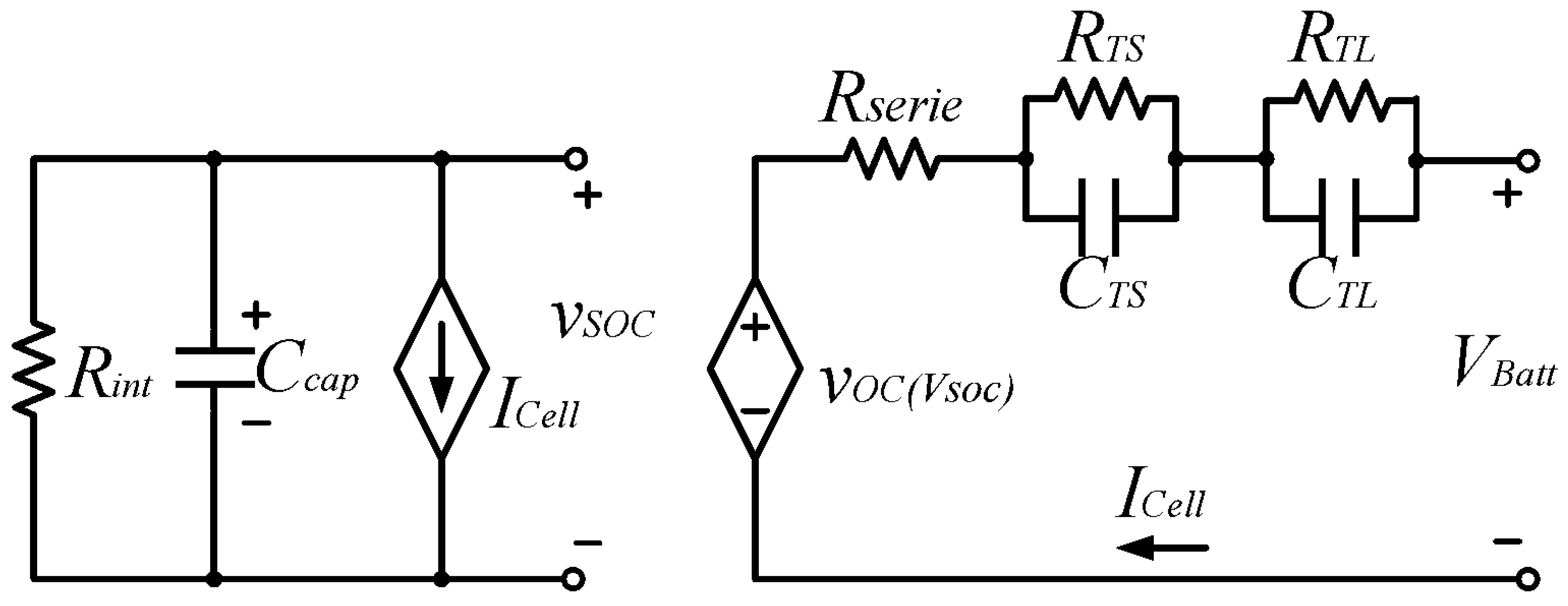
In [8], an ECM based on the Thevenin model (see Figure 1) was proposed to capture most of the nonlinear dynamics of the battery, including nonlinear open-circuit voltage, current-dependent capacity, cycle number, storage time, and transient response due to changes in the demand power. Although this model proves to be quite practical, it does not consider temperature changes or include the actual battery SoH, leading to a significant miscalculation of the SoC.

Figure 1.
Accurate 1RC Thevenin battery model [8,14,15].
3. Recursive Bayesian and Heuristic SoC Estimation Algorithms
Changes in temperature, current, and voltage strongly affect the performance of battery-based systems. These variations can introduce considerable errors in the ECM response. Estimation algorithms enable the adjustment of battery parameters to improve the matching between observed and predicted data, thereby enhancing the accuracy of the estimated SoC. In addition, these algorithms also allow for the estimation of the uncertainty associated with the predictions of the model. Table 1 describes the characteristics of some algorithms along with some research contributions reported in the literature.

Table 1.
Summary of recursive Bayesian and heuristic SoC estimation algorithms.
3.1. Kalman Filter-Based Methods
The Kalman filter (KF) is commonly used as an SoC estimation technique. It is particularly useful for handling a certain degree of uncertainty and provides weighted estimates. Moreover, it allows the adjustment of estimates after changes in the system conditions or battery characteristics. Depending on the desired characteristics of the SoC estimation, some variants of the KF have been developed. Finally, although the KF can handle nonlinear systems, sometimes linearization of the model is required, potentially introducing errors in the estimation [27].
3.2. Heuristic Algorithms in SoC Estimation
Heuristic techniques employed for SoC estimation in LIBs have gained significant attention in recent years, primarily because they do not explicitly need a model to represent the system dynamics. The strategies delineated in the existing literature following this approach focus on scanning the input–output relationship to assess the proposed system [28]. Generally, these algorithms showcase remarkable attributes such as high adaptability, nonlinear mapping, flexibility, machine learning capabilities, scalability, noise handling prowess, and an empirical orientation. Within the domain of SoC estimation, these methodologies focus on crucial aspects such as data collection, model training, and the eventual identification of parameters of interest [15]. They are typically used during the discharge process and leverage variables such as demand current, terminal voltage, and battery temperature as key determinants.
3.3. Hybrid Methods
The application of combined approaches has also been considered mainly to increase the accuracy and robustness in the estimation of the SoC. In this case, an optimization strategy is used to incorporate both model-based and data-based methods, achieving improvements in performance and obtaining more accurate results [29,30]. The most popular combined approaches include particle swarm optimization (PSO), genetic algorithms (GAs), and combinations using neural networks (NNs) and Thevenin equivalent circuits [31].
4. Methodology
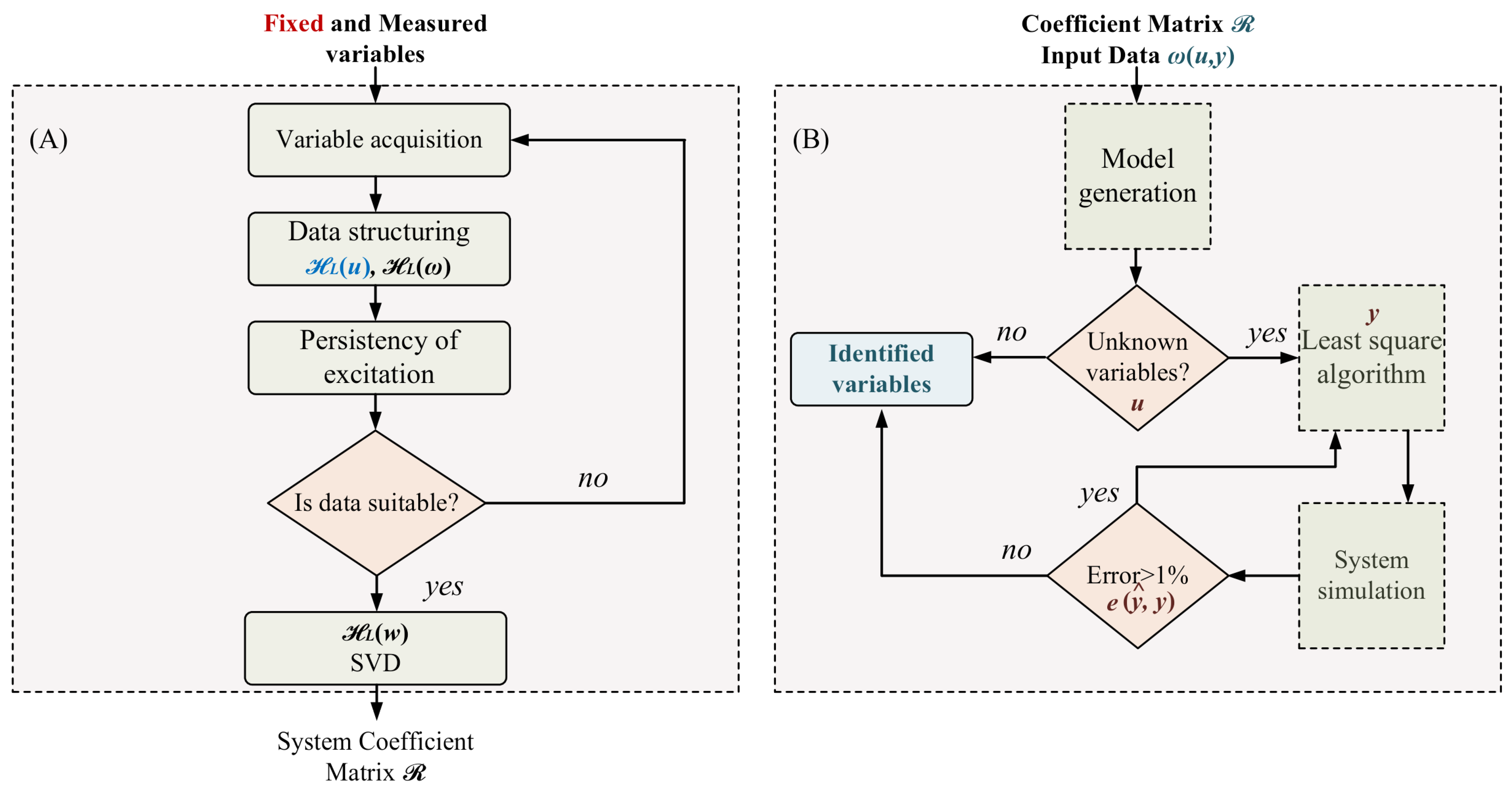
In this section, we outline the proposed data-driven modeling approach. For this, a model is built by gathering and analyzing the measured data from an LIB. The resulting model takes the form of a state-space representation characterizing the battery behavior. Figure 2 illustrates the overall process, comprising the following two main parts: Part A focuses on data gathering, structuring, and analysis; while part B addresses the model selection, validation, and implementation.
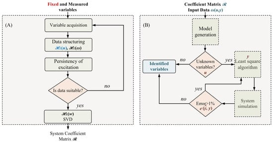
Figure 2.
Block diagram of the data-driven parameter identification algorithm. (A) Data acquisition and processing; identification of the matrix. (B) Identification, validation, and estimation of unknown system variables.
4.1. Data-Based System Modeling
Control systems can automatically adapt and adjust their operation to optimize performance, improve efficiency, and ensure safe operation by collecting and analyzing real-time data. The data-driven approach is a methodology based on acquiring specific data from the system under evaluation. In the data acquisition process, it is crucial to ensure that the sampling time is aligned with the system’s dynamics and to establish an optimal sampling window. The available measurement data vector is comprised of inputs and outputs , where the length is T and corresponds to the sequence of the series. Then, we can define a finite-dimensional signal vector space as , and it is classified and stored in a mapping discrete-time vector , that is,
For linear, time-invariant, continuous-time systems, the system’s behavior can be accurately represented through differential equations. A dynamical system is referred to as if it is a linear vector subspace that encapsulates the system’s behavior within and remains invariant over time, under the following conditions:
This characteristic guarantees that the system’s behavior stays unchanged over time [32,33]. Numerous systems can be modeled using differential equations and take the general form
In this context, and represent functions that describe the dynamics of the system. A specific representation of a linear, time-invariant, continuous-time differential system is defined by the solution set of a system of linear differential equations with constant coefficients [32]:
This uses constant matrices , which encapsulate the information related to the system’s state trajectories. Alternatively, if we treat the derivatives in Equation (4) as a finite difference approximation, the system can be expressed in the discrete domain as
where N is the maximum degree of the derivative and (with ) contains the information corresponding to the variables of the system and will help to find the state representation [32,34]. Expression (5) can also be described as a kernel representation in terms of the shift operator , this operator can be applied to a function in the form . This results in
where N is the maximum degree of the shift operator and ]. Note that to solve (6) it is necessary to find the value of the coefficient matrix . To achieve this, the following two Hankel matrices are constructed:
where , with N being determined by the number of states in the system. The matrix contains the vector associated with the system input. It is used to determine whether the measurement data can fully reveal the behavior of the system, in other words, if they are persistently exciting of order L, which yields a full row rank [35].
If the data are acceptable, then a singular value decomposition (SVD) of with dimensions is performed, which generates three simple matrices, and thus, its SVD is expressed as
where is a diagonal matrix that contains singular values and has the form
with and being orthogonal. If (9) is left-side multiplied by , then
This means that contains some values, referred to as annihilators, that make the values in zero, and thus, it can be partitioned as , where concentrates such annihilators. Moreover, from (6), it can be deduced that is also an annihilator, and thus,
with of dimension , , and . Once has been identified, the next step consists of partitioning the matrix as follows:
From (6), and based on partition (13), the resulting equation is given by
whose maximum delay degree is now constrained by the length of L.
From (14), a space mapping can be obtained through a technique called shift and cut [32], which applies a time displacement to obtain the system state variables as follows:
The resulting set of equations in (15) are used to approximate a state-space representation of the system. Applying a delay operator , and using (14), the resulting system can be expressed as
Consider the output equation in (15) , where . To ensure the operation is valid, must be partitioned into with and ; notice that is always square.
The output equation is obtained after developing the last equation of the state vector description (15), this yields
The resulting expression for the output equation, in the form analogous to (in continuous time), can be recovered by multiplying the state vector x by the output matrix , and adding the contribution of the input u multiplied by the direct transmission matrix , which yields
This expression describes how the states and inputs influence the output of the system. In summary, the state-space representation is given by (16) and (18).
Furthermore, based on the representations (16) and (18), it is possible to compute the system’s eigenvalues along with its time constant. This requires the computation of matrix A out of the generated system given by
which can be rewritten as
Now, considering that the state equation structure of a finite difference system is
then matrix and B turns out to be
4.2. Linear Recursive Estimator
The use of an estimation algorithm is suggested if one of the input variables is unknown, which typically happens with the OCV when trying to model batteries; these can be considered tracking problems in a similar way to how they are described in [33,36]. In the present work, a recursive least-squares algorithm is preferred for this task given its simplicity. It is important to note that the notation used in this particular section is only intended to illustrate the structure of the estimator that is used.
A set of noisy signals measured at a discrete time instant n and collected in a vector can be represented by the following linear combination:
where is the system state, is an matrix representing the impulse response; is the noise; and thus, the term contains the projected values [37,38].
Consider now the following general recursive least-squares estimator [33,39,40]:
where is the estimate, and is the estimator gain matrix. Notice that (23) is formed by two elements, namely, an estimated term , and a correction term for future approximations that involves the prediction error, that is,
where the matrix , whose diagonal values represent the variance of the model parameters, serves as a reference to quantify the uncertainty of the parameters to be estimated and of the observations of the system. It is a simplified variant of the Riccati equation aimed at minimizing the mean squared error between the observations and the model predictions. While the matrix helps to determine how much the model parameters adjust in response to new observations, the contribution of this matrix depends on the uncertainty in the system parameters. This matrix is used to quantify the uncertainty in the estimated model parameters. This matrix is expressed as follows [39,41]:
Finally, the error variable is given by
This estimator allows a fine-tuning of the acquired model to establish the connection between independent variables and the dependent variable, which is currently unknown. The outcome of this process yields optimal parameter values for the refined model. Once these values are determined, the model is adjusted and can then be used to forecast outcomes for new observations.
5. Experiments and Results Discussion
5.1. Battery Model Identification
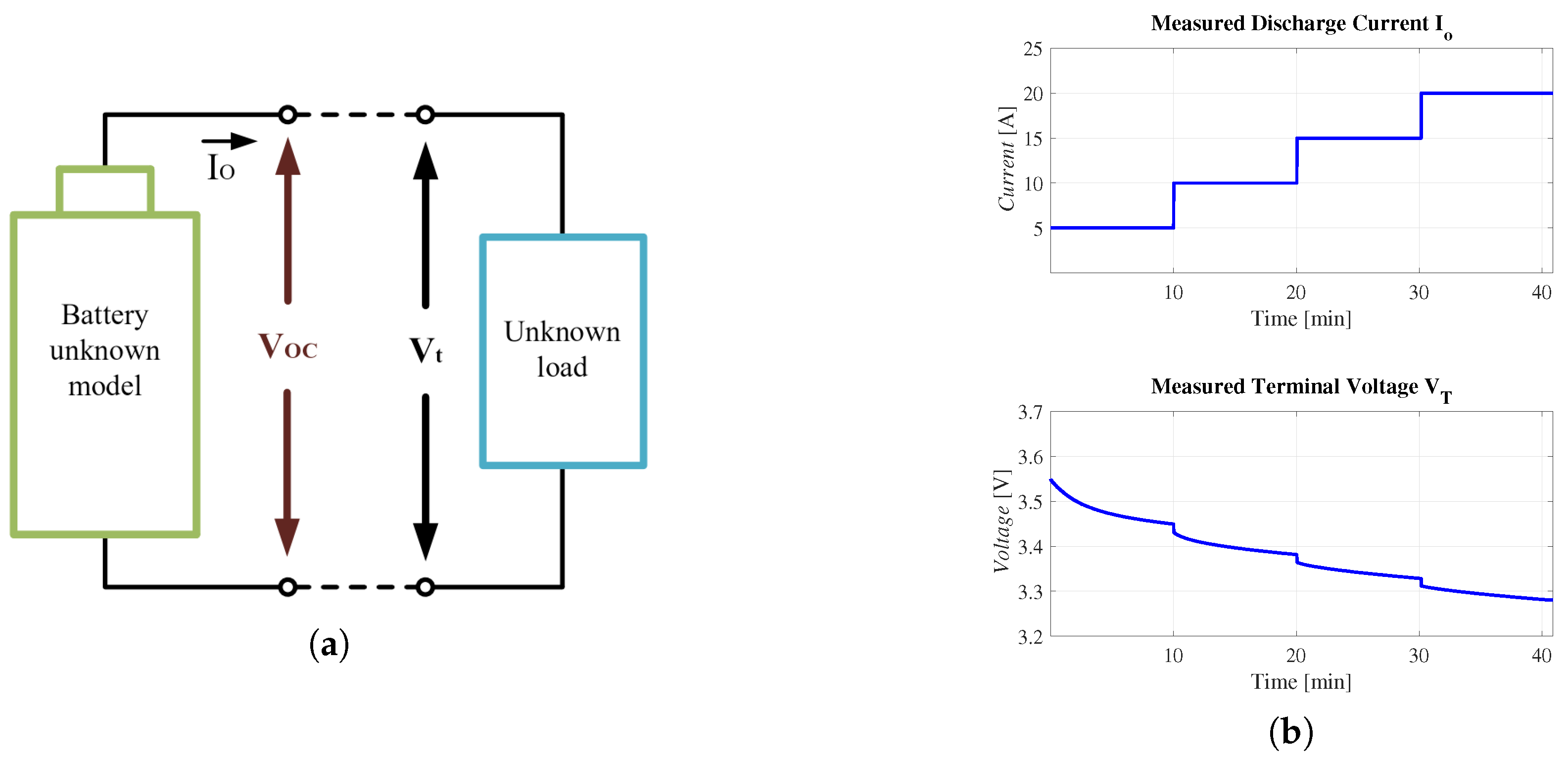
Consider the system shown in Figure 3a, which comprises a battery and an unknown load. The parameters of interest to obtain a state-space system representation are, in this case, the open-circuit voltage , terminal voltage , and discharge current .

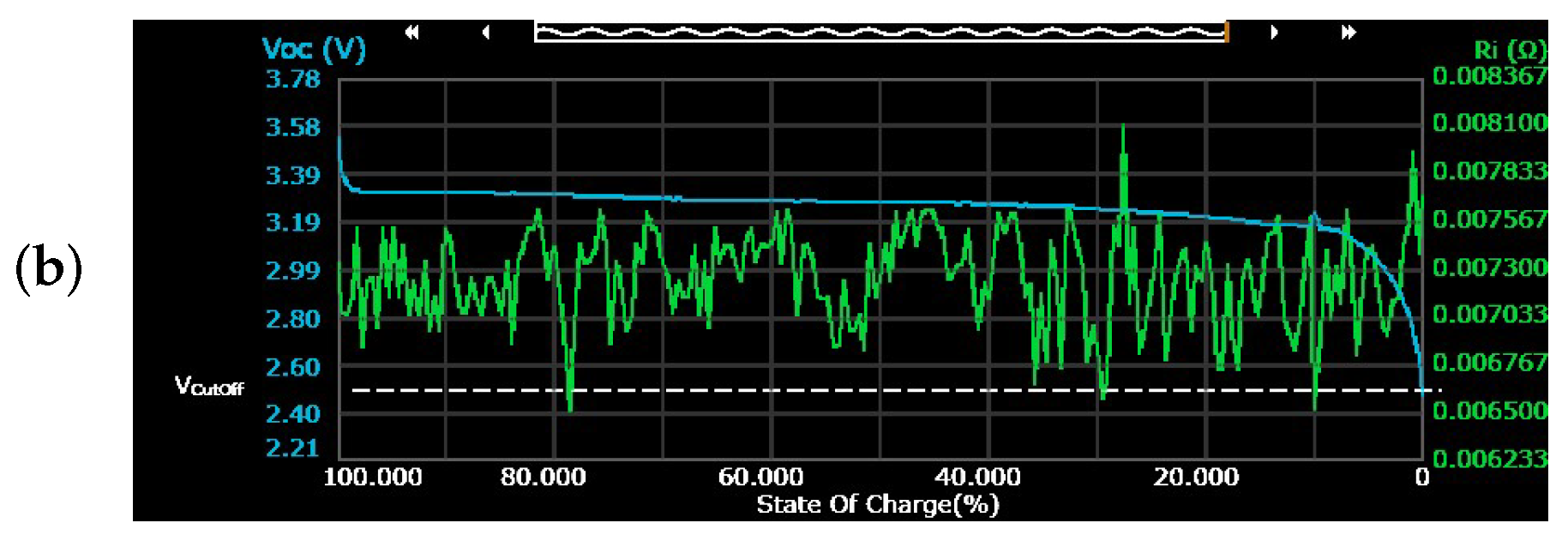
Figure 3.
(a) Unknown system battery/load for parameter identification, and (b) (from top to bottom) discharge step current and battery terminal voltage .
The vector of input variables is defined as , while the output is defined as . In the input vector u, is considered an unknown constant, which, for testing purposes, is fixed at 3.6 V.
Data for and were obtained during cell discharge, where a lithium-ion cell model CA100FI was used. The discharge current profile consisted of a series of pulses of 5, 10, 15, and 20, programmed every 10 min in an electronic load BK 8600, with Hz. The data acquisition was performed using external sensing provided by the electronic load and processed using Matlab 2023b. The responses are shown in Figure 3b.
To size the Hankel matrices and , a maximum length for the states is proposed, while the system has only one input; hence, . Finally, the dimension of the coefficient matrix is , resulting in a partition that only includes and . Thus, the state-space representation of the system is given by
Additionally, Table 2 displays the coefficients of , along with the eigenvalues and time constants of the battery. These values were calculated through measurements at different SoCs.
Table 2.
Coefficient values of and battery time constants under different SoCs.
Although the model obtained in (29) optimally approximates the battery time response, it considers a constant OCV (). This parameter must be estimated to ensure a better match of the model against the real system and to allow for a simpler calculation of the SoC based on the OCV. For this, the output model equation is expressed as its counterpart in the continuous-time state-space model , that is,
Notice that there are two unknown variables, and . Based on this, a new estimation vector variable is defined that involves estimates for these two unknown variables, that is,
Now, defining as a constant vector that contains part of the coefficient matrix , and as the extended vector of variables to estimate, that is,
then the new output equation of the proposed model can be written in terms of the estimated variables as follows:
Out of this, (25) can be rewritten in terms of to estimate as follows:
where the estimator gain matrix and the covariance error matrix in (26) can be reconstructed as
while the error variable is given by
Finally, the identified model for the battery turns out to be
where and contain the estimated variable .
5.2. Experimental Validation
To validate the models obtained in the previous section, three different scenarios were proposed. The first test scenario was conducted under various SoC conditions to verify that the identification of the coefficient matrix is not affected by the lack of information of . The second test is performed under the condition of full discharge at constant current. The third scenario involves a full discharge condition with step-like transitions in the discharge current. These scenarios are executed with the identified model (38), and performing the estimation of . All discharge processes were carried out using the Keysight RP7971A battery emulator, shown in Figure 4a.
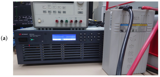
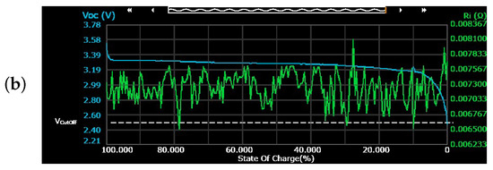
Figure 4.
(a) Keysight battery emulator and cell used in the discharge test, and (b) OCV and plots obtained via the Keysight BenchVue 2022.1 software.
It is worth noting that all charge/discharge processes were performed following the procedure established in the IEC 62660-1 [42] and ISO 12405-4 [43] international standards.
5.2.1. Test 1—Model Validation
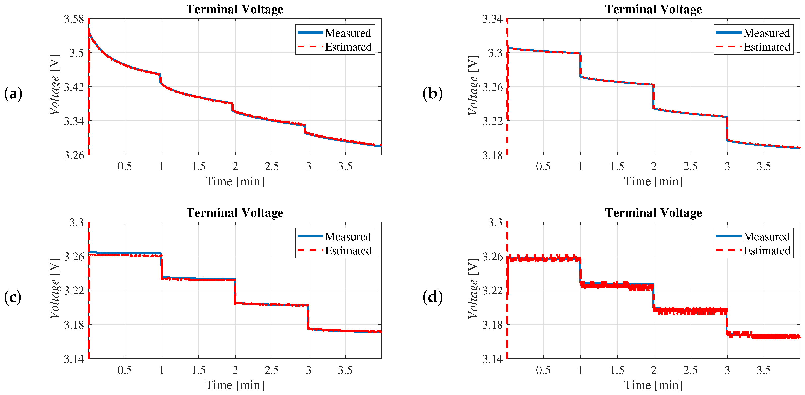
To validate the model (29), subject to an unknown (one of the input variables), the measured battery terminal voltage at different SoCs is compared with the corresponding variable generated by the model. This comparison is shown in Figure 5. During this test scenario, the data were acquired over a period of 4 min, with stepped transitions in the discharge current of , 5, , and 10 A, and for different SoCs of , , , and .
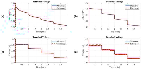
Figure 5.
Comparison of waveforms of the measured terminal voltage with those generated by the model in (1) for different states of charge: (a) , (b) , (c) , and (d) .
Note that in Figure 5 the terminal voltage generated by the model, where is considered a constant parameter, closely approximates the measured voltage. However, the convergence of towards its real value is more linear when significant transitions occur in the discharge current . This shows that even without knowing the exact value of , as part of the excitation to identify matrix , this estimate is quite close to the real battery response. Consequently, this approximate model is useful to estimate from the output equation.
5.2.2. Test 2—Constant Current Discharge
The first discharge condition was established at constant currents of 25 A and 50 A. The second test condition was performed using a step-like discharge current that fluctuated between 25 A and 50 A, where the transition lasted 10 min from one to the other. The measured data were obtained using Keysight BenchVue software. The total time elapsed to complete the discharge process was approximately 250 min.
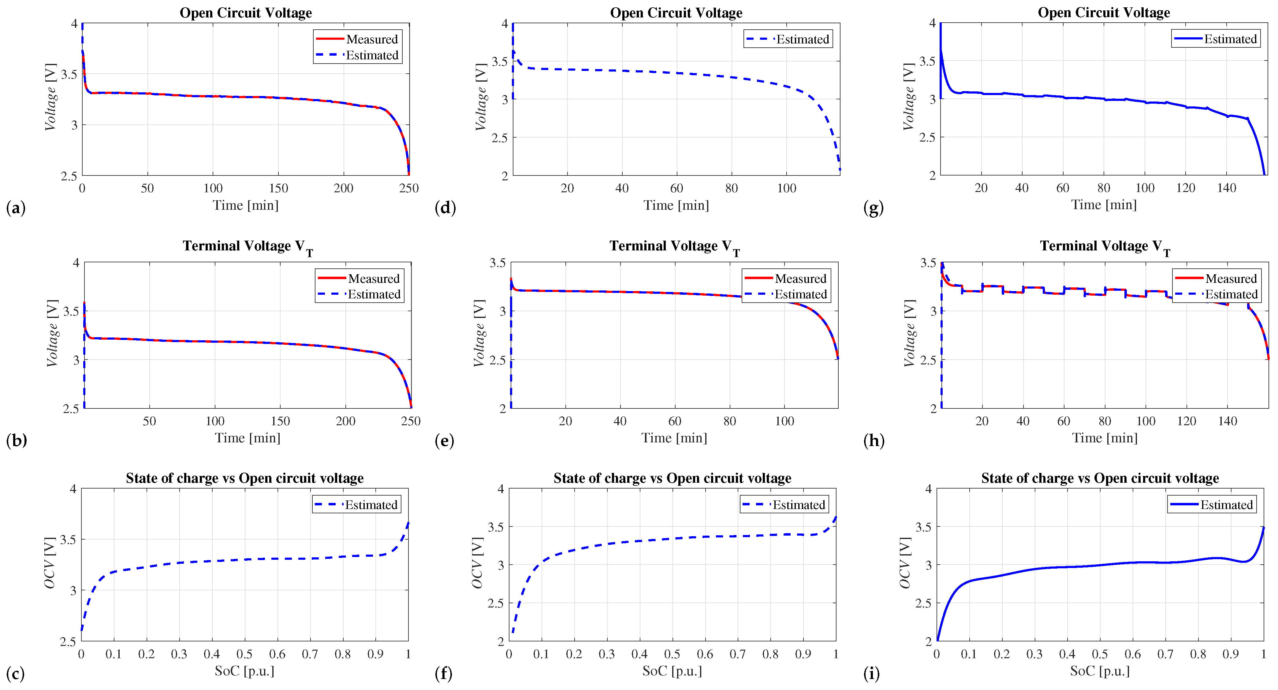
Figure 6a shows the comparison between the measured and estimated OCV at a constant discharge current of 25 A. The data for the OCV were acquired using the Keysight battery emulator. Figure 6b presents the measured and estimated waveforms for ; and Figure 6c shows the SoC versus OCV plot. The SoC presented in Figure 6 was computed from the discharge current and adjusted through a polynomial fitting based on the estimated .
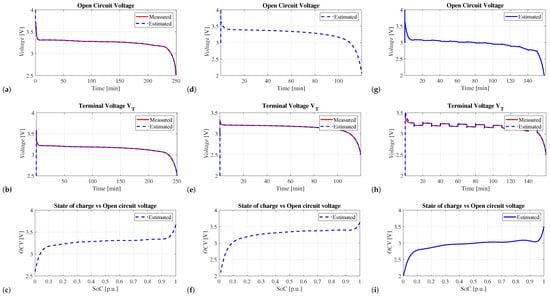
Figure 6.
(From top to bottom) Time responses of , , and the response of SoC against OCV, for constant discharge currents of 25 A (a–c) and 50 A (d–f), and a step-like current fluctuating between 25 A and 50 A (g–i).
The second discharge condition was carried out at a constant current of 50 A, for which an undervoltage limit of 2 V for OCV was set according to the manufacturer’s specifications. The total duration of the test was approximately 120 min. Figure 6d–f shows the graphs for the voltages , , and the SoC. Figure 6e presents a comparison between the measured and estimated voltages. It can be seen that the estimation of for both discharge conditions exhibits higher accuracy when incorporating the estimation of . Furthermore, the estimation is now free of noise compared to the condition in which is considered a constant vector.
5.2.3. Test 3—Step-like Transition Current Discharge
The last test considered a step-change discharge current with values of 25 A and 50 A, where the transition lasted 10 min from one to the other. The results are shown in Figure 6g–i. Notice that despite the current discharge transitions, the model is capable of following the trajectories and optimally tracking the voltage . The estimation of during this test is not affected by the transitions in , as it does not show oscillations or perceptible transitions that affect the performance of this estimate. Furthermore, during this discharge scenario, it is observed that for SoC values below the estimation provided by the model shows that the difference between the measured and estimated is quite accurate, in contrast to network electrical models, where as the battery approaches full discharge, the curve begins to diverge from the real curve. This could help a battery management system to have better control over the remaining energy available in batteries that operate with a low SoC.
5.2.4. Estimator Error Values
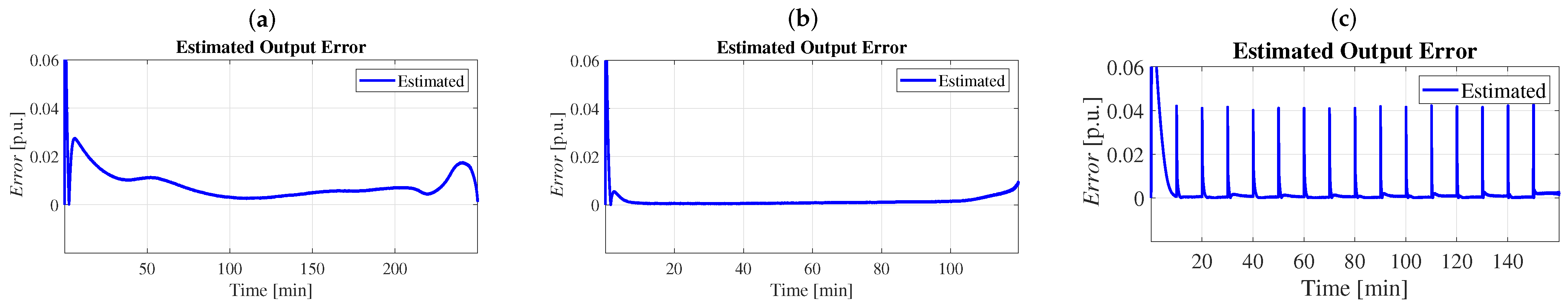
Figure 7 presents a graph of the error between the measured and estimated value of . This error is critical because, in the absence of the actual OCV measurement, a small value in the error indicates that the calculated OCV is close to the real one. This idea is supported by the fact that the generated output parameter includes both the OCV and the hidden state of the system.

Figure 7.
Time response of the error between the estimated and measured voltage for constant discharge currents of (a) 25 A and (b) 50 A, and (c) a step-like discharge current fluctuating between 25 A and 50 A.
Furthermore, the most significant difference in the estimated occurs when the battery has an SoC close to or , which corresponds to a faster transition of , commonly known as the nonlinear regions of the OCV curve. This indicates that convergence towards the real value is not too fast, which is due to the nature of the considered estimator.
6. Conclusions
This article proposed a data-driven methodology for battery modeling without the need for an equivalent electrical model and that involves just a few measurements. This methodology enables the recognition of the system trajectories, which are determined by the coefficient matrix , by applying controlled changes in the input signal and observing the output signal . From this process, a set of difference equations is generated to approximate the real behavior of the battery.
Using the generated model that considers as a constant vector, an estimation of was performed using a modified least-squares algorithm. Subsequently, this data vector was used to adjust the SoC curve. The model validation, as well as estimator validation, were carried out using different current discharge conditions in the battery and comparing the model output with the actual measurements. The experimental results showed that the battery trajectories of the generated model can closely follow the trajectories of the real system, providing a fairly accurate estimation of and SoC with minimal measurements and computational cost.
Author Contributions
Conceptualization, G.E. and J.E.V.-R.; methodology, D.G. and J.C.R.-C.; validation, E.D.S.-V. and J.E.V.-R.; formal analysis, E.D.S.-V. and J.E.V.-R.; investigation, E.D.S.-V. and J.M.S.; writing, E.D.S.-V., G.E., J.E.V.-R. and J.C.R.-C.; review and editing, D.G., J.M.S., G.E. and J.C.R.-C. All authors have read and agreed to the published version of the manuscript.
Funding
This research and the APC was funded in part by CONAHCYT grant number CF-2023-G-1344 and Tecnológico de Monterrey.
Data Availability Statement
Data are contained within the article.
Acknowledgments
We Authors would like to thank CONAHCYT for their support through the project CF-2023-G-1344 Desarrollo de nuevos enfoques para analisis, modelado y control de convertidores electronics. Also, want to thank Tecnológico de Monterrey for the APC support.
Conflicts of Interest
The authors declare no conflicts of interest.
References
- Cao, Y.; Kroeze, R.C.; Krein, P.T. Multi-timescale parametric electrical battery model for use in dynamic electric vehicle simulations. IEEE Trans. Transp. Electrif. 2016, 2, 432–442. [Google Scholar] [CrossRef]
- Feng, F.; Hu, X.; Liu, K.; Che, Y.; Lin, X.; Jin, G.; Liu, B. A practical and comprehensive evaluation method for series-connected battery pack models. IEEE Trans. Transp. Electrif. 2020, 6, 391–416. [Google Scholar] [CrossRef]
- Lee, K.Y.; Vale, Z.A. Applications of Modern Heuristic Optimization Methods in Power and Energy Systems; John Wiley & Sons: Hoboken, NJ, USA, 2020. [Google Scholar]
- Qays, M.O.; Buswig, Y.; Hossain, M.L.; Abu-Siada, A. Recent progress and future trends on the state of charge estimation methods to improve battery-storage efficiency: A review. CSEE J. Power Energy Syst. 2020, 8, 105–114. [Google Scholar]
- Chen, R.; Fan, Y.; Yuan, S.; Hao, Y. Vehicle Collaborative Partial Offloading Strategy in Vehicular Edge Computing. Mathematics 2024, 12, 1466. [Google Scholar] [CrossRef]
- Hussein, A.A.H.; Batarseh, I. An overview of generic battery models. In Proceedings of the 2011 IEEE Power and Energy Society General Meeting, Detroit, MI, USA, 24–28 July 2011; pp. 1–6. [Google Scholar]
- Hasan, R.; Scott, J. Extending randles’s battery model to predict impedance, charge—Voltage, and runtime characteristics. IEEE Access 2020, 8, 85321–85328. [Google Scholar] [CrossRef]
- Chen, M.; Rincon-Mora, G.A. Accurate electrical battery model capable of predicting runtime and IV performance. IEEE Trans. Energy Convers. 2006, 21, 504–511. [Google Scholar] [CrossRef]
- Rimpas, D.; Kaminaris, S.D.; Piromalis, D.D.; Vokas, G. Real-Time Management for an EV Hybrid Storage System Based on Fuzzy Control. Mathematics 2023, 11, 4429. [Google Scholar] [CrossRef]
- Liu, X.; Li, W.; Zhou, A. PNGV equivalent circuit model and SOC estimation algorithm for lithium battery pack adopted in AGV vehicle. IEEE Access 2018, 6, 23639–23647. [Google Scholar] [CrossRef]
- Jung, S.; Tullu, A. Characteristics Evaluation of 14 Battery Equivalent Circuit Models. IEEE Access 2023, 11, 117200–117209. [Google Scholar] [CrossRef]
- Liu, S.; Dong, X.; Zhang, Y. A new state of charge estimation method for lithium-ion battery based on the fractional order model. IEEE Access 2019, 7, 122949–122954. [Google Scholar] [CrossRef]
- Wang, J.; Zhang, L.; Mao, J.; Zhou, J.; Xu, D. Fractional order equivalent circuit model and SOC estimation of supercapacitors for use in HESS. IEEE Access 2019, 7, 52565–52572. [Google Scholar] [CrossRef]
- Kim, W.; Lee, P.Y.; Kim, J.; Kim, K.S. A robust state of charge estimation approach based on nonlinear battery cell model for lithium-ion batteries in electric vehicles. IEEE Trans. Veh. Technol. 2021, 70, 5638–5647. [Google Scholar] [CrossRef]
- Larijani, M.R.; Kia, S.H.; Zolghadri, M.; El Hajjaji, A.; Taghavipour, A. Linear Parameter-Varying Model Predictive Control for Intelligent Energy Management in Battery/Supercapacitor Electric Vehicles. IEEE Access 2024, 12, 51026–51040. [Google Scholar] [CrossRef]
- Shrivastava, P.; Soon, T.K.; Idris, M.Y.I.B.; Mekhilef, S.; Adnan, S.B.R.S. Combined state of charge and state of energy estimation of lithium-ion battery using dual forgetting factor-based adaptive extended Kalman filter for electric vehicle applications. IEEE Trans. Veh. Technol. 2021, 70, 1200–1215. [Google Scholar] [CrossRef]
- Zhu, Q.; Xu, M.; Liu, W.; Zheng, M. A state of charge estimation method for lithium-ion batteries based on fractional order adaptive extended kalman filter. Energy 2019, 187, 115880. [Google Scholar] [CrossRef]
- Wadi, A.; Abdel-Hafez, M.F.; Hussein, A.A.; Alkhawaja, F. Alleviating dynamic model uncertainty effects for improved battery SOC estimation of EVs in highly dynamic environments. IEEE Trans. Veh. Technol. 2021, 70, 6554–6566. [Google Scholar] [CrossRef]
- Feng, K.; Li, J.; Zhang, D.; Wei, X.; Yin, J. Robust Central Difference Kalman Filter with Mixture Correntropy: A Case Study for Integrated Navigation. IEEE Access 2021, 9, 80772–80786. [Google Scholar] [CrossRef]
- Partovibakhsh, M.; Liu, G. An adaptive unscented Kalman filtering approach for online estimation of model parameters and state-of-charge of lithium-ion batteries for autonomous mobile robots. IEEE Trans. Control. Syst. Technol. 2014, 23, 357–363. [Google Scholar] [CrossRef]
- Zhang, X.; Wang, Y.; Yang, D.; Chen, Z. An on-line estimation of battery pack parameters and state-of-charge using dual filters based on pack model. Energy 2016, 115, 219–229. [Google Scholar] [CrossRef]
- Arasaratnam, I.; Haykin, S.; Hurd, T.R. Cubature Kalman filtering for continuous-discrete systems: Theory and simulations. IEEE Trans. Signal Process. 2010, 58, 4977–4993. [Google Scholar] [CrossRef]
- Shu, X.; Li, G.; Zhang, Y.; Shen, S.; Chen, Z.; Liu, Y. Stage of charge estimation of lithium-ion battery packs based on improved cubature Kalman filter with long short-term memory model. IEEE Trans. Transp. Electrif. 2020, 7, 1271–1284. [Google Scholar] [CrossRef]
- Wang, D.; Yang, F.; Tsui, K.L.; Zhou, Q.; Bae, S.J. Remaining useful life prediction of lithium-ion batteries based on spherical cubature particle filter. IEEE Trans. Instrum. Meas. 2016, 65, 1282–1291. [Google Scholar] [CrossRef]
- How, D.N.; Hannan, M.A.; Lipu, M.S.H.; Sahari, K.S.; Ker, P.J.; Muttaqi, K.M. State-of-charge estimation of li-ion battery in electric vehicles: A deep neural network approach. IEEE Trans. Ind. Appl. 2020, 56, 5565–5574. [Google Scholar] [CrossRef]
- Li, S.G.; Sharkh, S.M.; Walsh, F.C.; Zhang, C.N. Energy and battery management of a plug-in series hybrid electric vehicle using fuzzy logic. IEEE Trans. Veh. Technol. 2011, 60, 3571–3585. [Google Scholar] [CrossRef]
- Ma, Y.; Liu, D. An Adaptive Cubature Kalman Filter Based on Resampling-Free Sigma-Point Update Framework and Improved Empirical Mode Decomposition for INS/CNS Navigation. Mathematics 2024, 12, 1607. [Google Scholar] [CrossRef]
- Kadem, O.; Kim, J. Real-time state of charge-open circuit voltage curve construction for battery state of charge estimation. IEEE Trans. Veh. Technol. 2023, 72, 8613–8622. [Google Scholar] [CrossRef]
- Su, S.; Li, W.; Mou, J.; Garg, A.; Gao, L.; Liu, J. A hybrid battery equivalent circuit model, deep learning, and transfer learning for battery state monitoring. IEEE Trans. Transp. Electrif. 2022, 9, 1113–1127. [Google Scholar] [CrossRef]
- Guo, R.; Shen, W. A model fusion method for online state of charge and state of power co-estimation of lithium-ion batteries in electric vehicles. IEEE Trans. Veh. Technol. 2022, 71, 11515–11525. [Google Scholar] [CrossRef]
- How, D.N.; Hannan, M.; Lipu, M.H.; Ker, P.J. State of charge estimation for lithium-ion batteries using model-based and data-driven methods: A review. IEEE Access 2019, 7, 136116–136136. [Google Scholar] [CrossRef]
- Rapisarda, P.; Willems, J.C. State maps for linear systems. SIAM J. Control. Optim. 1997, 35, 1053–1091. [Google Scholar] [CrossRef]
- Balakrishnan, V. System Identification: Theory for the User: Lennart Ljung; Prentice-Hall: Englewood Cliffs, NJ, USA, 1999; ISBN 0-13-656695-2. [Google Scholar]
- Rivera, D.; Guillen, D.; Mayo-Maldonado, J.C.; Valdez-Resendiz, J.E.; Escobar, G. Power grid dynamic performance enhancement via statcom data-driven control. Mathematics 2021, 9, 2361. [Google Scholar] [CrossRef]
- Willems, J.C.; Rapisarda, P.; Markovsky, I.; De Moor, B.L. A note on persistency of excitation. Syst. Control. Lett. 2005, 54, 325–329. [Google Scholar] [CrossRef]
- Hao, L.; Wang, C.; Shi, Y. Quadratic Tracking Control of Linear Stochastic Systems with Unknown Dynamics Using Average Off-Policy Q-Learning Method. Mathematics 2024, 12, 1533. [Google Scholar] [CrossRef]
- Hänsler, E.; Schmidt, G. Acoustic Echo and Noise Control: A Practical Approach; John Wiley & Sons: Hoboken, NJ, USA, 2005; Chapter 7. [Google Scholar]
- Paleologu, C.; Benesty, J.; Ciochina, S. A robust variable forgetting factor recursive least-squares algorithm for system identification. IEEE Signal Process. Lett. 2008, 15, 597–600. [Google Scholar] [CrossRef]
- Simon, D. Optimal State Estimation: Kalman, H infinity, and Nonlinear Approaches; John Wiley & Sons: Hoboken, NJ, USA, 2006. [Google Scholar]
- Young, P.C. Recursive least squares estimation. In Recursive Estimation and Time-Series Analysis: An Introduction for the Student and Practitioner; Springer: Berlin/Heidelberg, Germany, 2011; pp. 29–46. [Google Scholar]
- Amaral, L.F.C.; Lopes, M.V.; Barros, A.K. A nonquadratic algorithm based on the extended recursive least-squares algorithm. IEEE Signal Process. Lett. 2018, 25, 1535–1539. [Google Scholar] [CrossRef]
- IEC. Secondary Lithium-Ion Cells for the Propulsion of Electric Road Vehicles—Part 1: Performance Testing; IEC 62660-1; IEC: Geneva, Switzerland, 2018. [Google Scholar]
- ISO 12405-4; Electrically Propelled Road Vehicles—Test Specification for Lithium-Ion Traction Battery Packs and Systems—Part 4: Performance Testing for High-Power Applications. ISO: Geneva, Switzerland, 2018.

Disclaimer/Publisher’s Note: The statements, opinions and data contained in all publications are solely those of the individual author(s) and contributor(s) and not of MDPI and/or the editor(s). MDPI and/or the editor(s) disclaim responsibility for any injury to people or property resulting from any ideas, methods, instructions or products referred to in the content. |
© 2024 by the authors. Licensee MDPI, Basel, Switzerland. This article is an open access article distributed under the terms and conditions of the Creative Commons Attribution (CC BY) license (https://creativecommons.org/licenses/by/4.0/).