
Enhancing Autism Spectrum Disorder Classification with Lightweight Quantized CNNs and Federated Learning on ABIDE-1 Dataset

 ,
,  , , ,
, , ,  and
and
Abstract
:1. Introduction
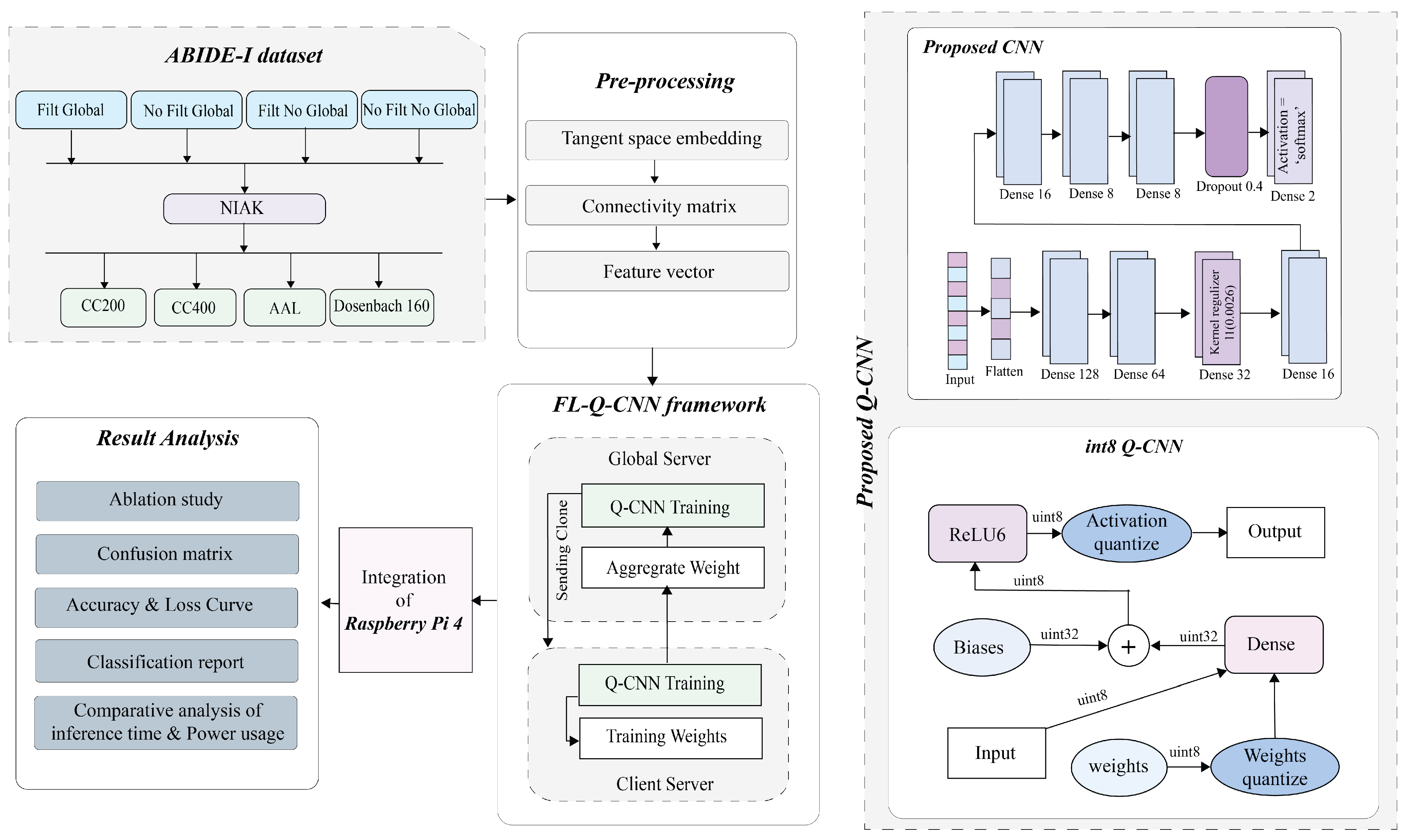
- A lightweight Q-CNN model is introduced through the utilization of int8 quantization technique.
- An FL-based framework is incorporated for the classification to preserve the privacy of healthcare centers and make the proposed approach more effective for real-world usage.
- The most effective atlas for ASD classification can be identified using the four filtering steps within the NIAK pipeline, with the CC200 brain atlas being found optimal.
- The proposed FL-Q-CNN model is implemented in the Raspberry pi 4 to evaluate its performance in real-world settings.
- A comparative analysis is carried out integrating the CNN model, float 16 quantization model, and proposed int8 Q-CNN model in the Raspberry Pi 4 by calculating the lowest inference time, flash occupancy, and power usage to demonstrate the effectiveness of the proposed framework.
2. Related Works
3. Background Knowledge
3.1. NeuroImaging Analysis Kit (NIAK) Pipeline
3.2. Brain Atlas
3.3. Filtering Methods
- Filt-global: Aims to enhance signal quality by combining temporal filtering and global signal regression.
- Nofilt-global: Focuses on removing global artifacts while retaining the full frequency spectrum.
- Filt-noglobal: Aims to preserve neural signals within the frequency range of interest, without removing the global signal.
- Nofilt-noglobal: Provides a baseline with no preprocessing, retaining all raw data components.
3.4. Quantization
4. Dataset Description
5. Proposed Method
5.1. Extraction of ROI
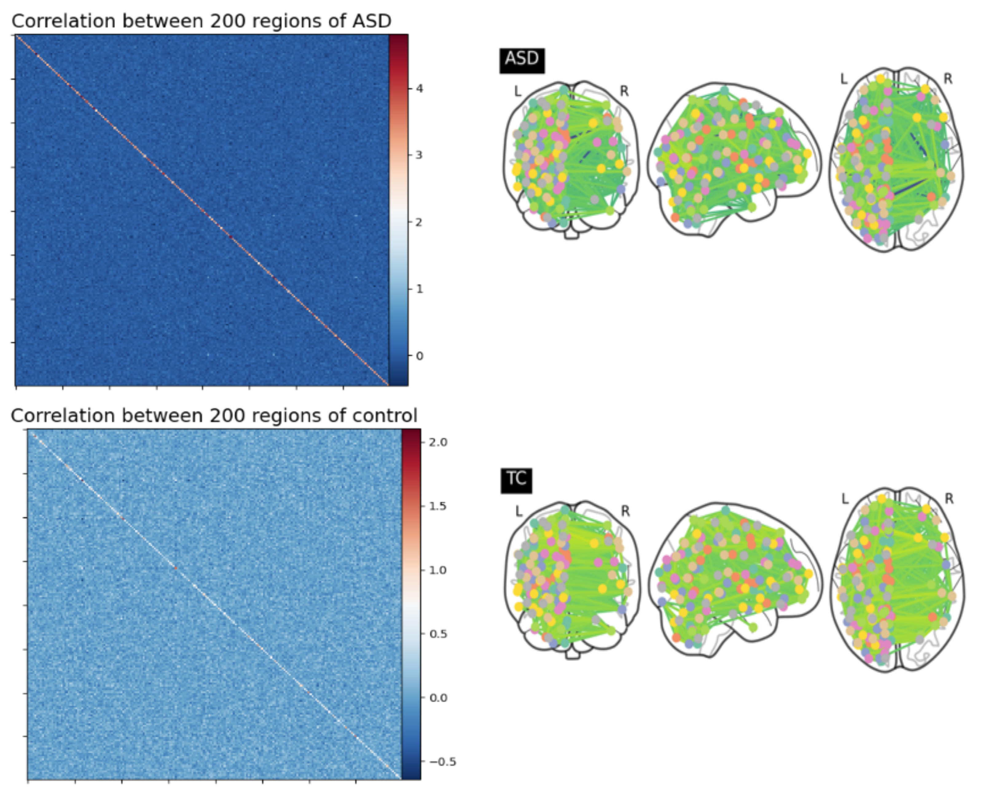
5.2. Formation of the Functional Connectivity Matrix
5.3. Conversion of Correlation Matrix to 1D Feature Vector
6. Proposed Model
6.1. CNN Model
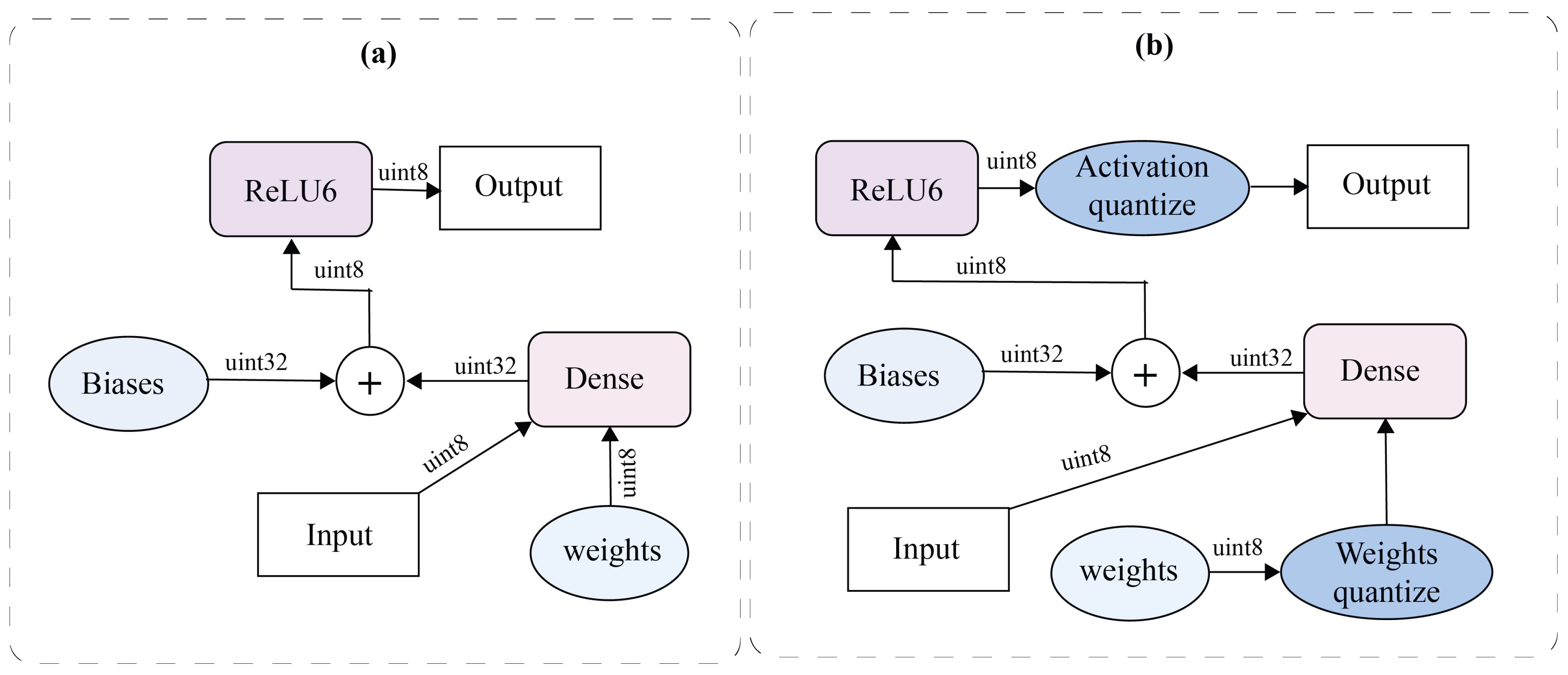
6.2. Proposed Q-CNN
| Algorithm 1 Quantization Training Process |
|
- Prior to performing convolution operations with the input, the weights were quantized. When batch normalization was applied, the batch normalization parameters were incorporated into the weights before quantization. This integration was achieved using Equation (9). Here, represents the scale parameter from batch normalization, is an estimated moving average of the variance of the convolutional results over the batch, w is the original weight, and is a small constant for numerical stability.
- Activation quantization was performed at specific points during inference, ensuring accurate approximation of activations. The quantization process for each layer was defined by several parameters, including the number of quantization levels and the clipping range. The quantization function q is shown in Equation (10).
6.3. Federated Learning Framework
6.4. Raspberry PI Configuration
7. Results
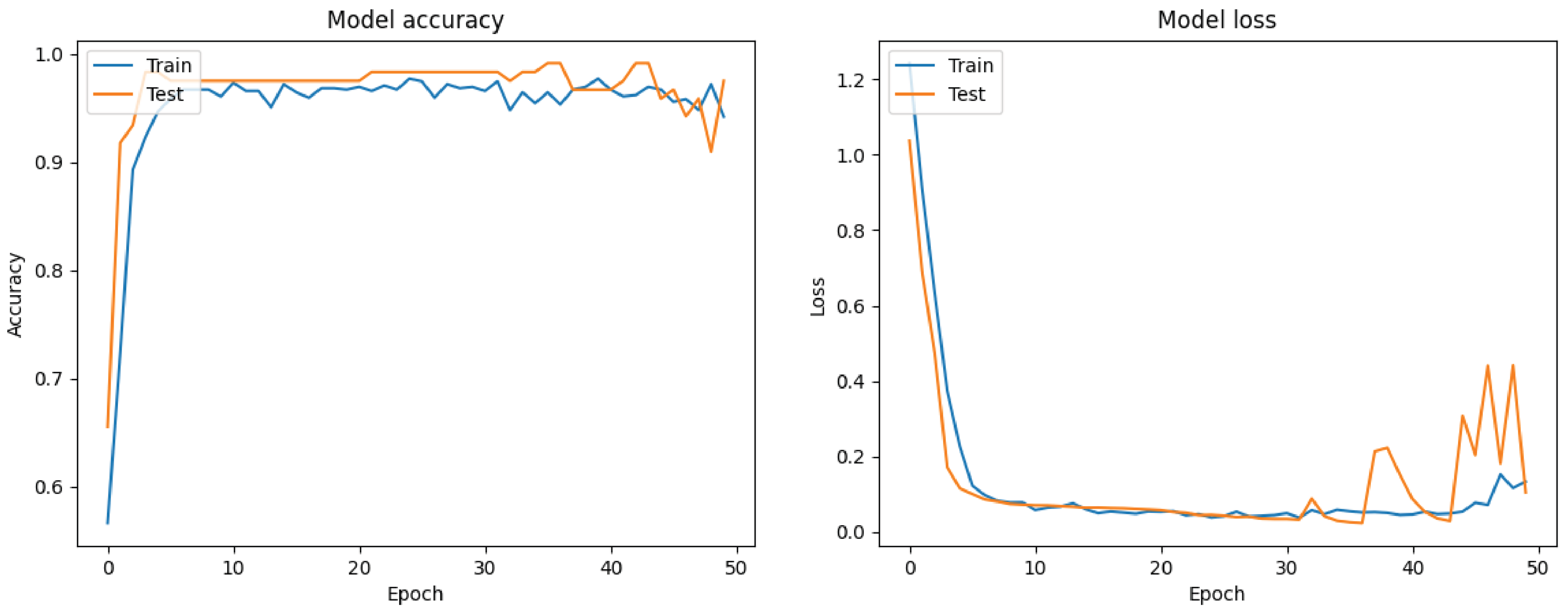
7.1. Filt-Global
7.2. Filt-Noglobal
7.3. Nofilt-Global
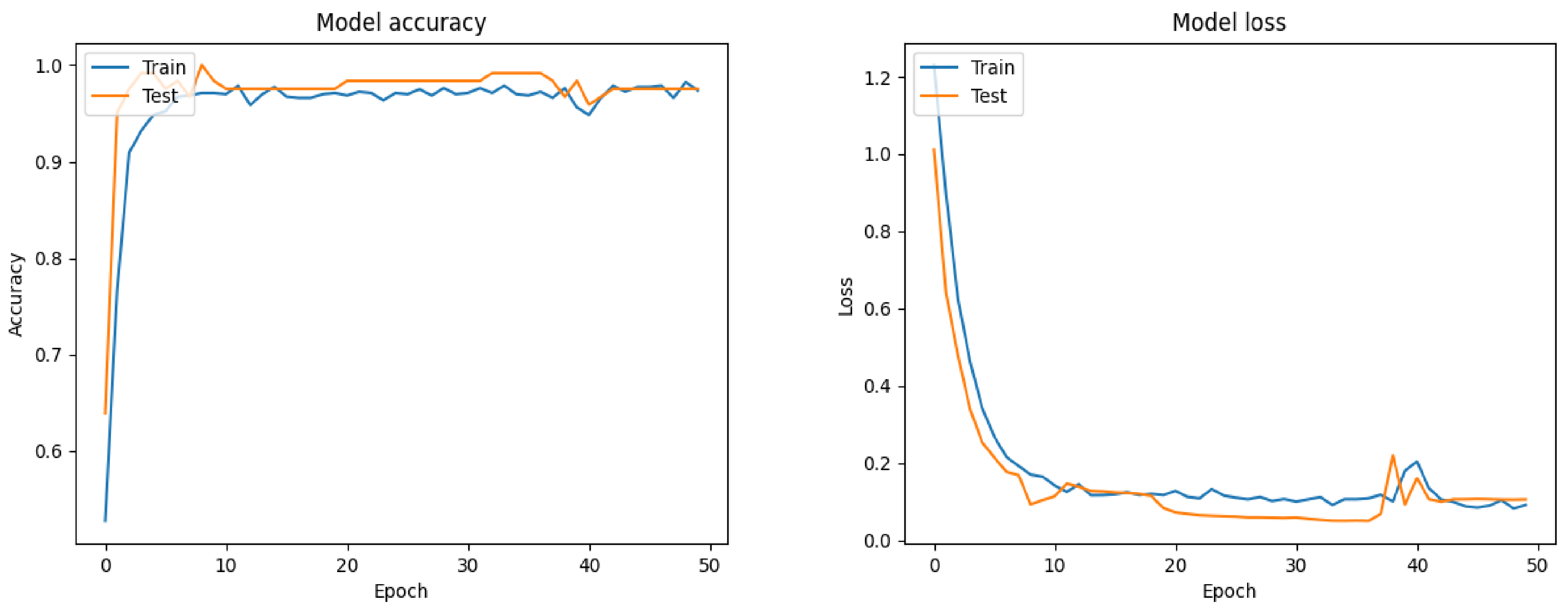
7.4. Nofilt-Noglobal
7.5. Computational Complexity Analysis of Local Machine
7.6. Computational Complexity Analysis of Raspberry PI
8. Limitations and Future Work
9. Conclusions
Author Contributions
Funding
Informed Consent Statement
Data Availability Statement
Conflicts of Interest
Abbreviations
| 1D | One-Dimensional |
| 3D-DEC | Three-Dimensional Deep Embedding Clustering |
| AAL | Automated Anatomical Labeling |
| ABIDE | Autism Brain Imaging Data Exchange |
| ADHD | Attention Deficit Hyperactivity Disorder |
| AdSDs | Adjustable Speed Drives |
| AI | Artificial Intelligence |
| ASD | Autism spectrum disorder |
| BOLD | Blood Oxygen Level-Dependent |
| CAD | Computer-Aided Diagnosis |
| CC200 | Craddock 200 |
| CC400 | Craddock 400 |
| CCS | Connectome Computation System |
| CNN | Convolutional Neural Network |
| CPAC | Configurable Pipeline for the Analysis of Connectomes |
| DeepASDPred | Deep learning-based autism spectrum disorder prediction |
| DNN | Deep Neural Network |
| DPABI | Data Processing and Analysis for Brain Imaging |
| 1D | One-Dimensional |
| DPARSF | Data Processing Assistant for Resting-State fMRI |
| EEG | Electroencephalography |
| EZ | Eickhoff–Zilles |
| FDR | False Discovery Rate |
| FL | Federated learning |
| FNR | False Negative Rate |
| FNU | Functional Neuroimaging Unit |
| fMRI | functional Magnetic Resonance Imaging |
| FPR | False Positive Rate |
| HO | Harvard–Oxford |
| LSTM | Long Short-Term Memory |
| MCC | Matthews Correlation Coefficient |
| MLP | Multilayer Perceptron |
| MNI | Montreal Neurological Institute |
| NIAK | NeuroImaging Analysis Kit |
| NPV | Negative Predictive Value |
| PCP | Preprocessed Connectomes Project |
| QAP | Quality Assessment Protocol |
| QAT | Quantize Aware Training |
| Q-CNN | Quantized Convolutional Neural Network |
| ReLU | Rectified Linear Unit |
| RNA | Ribonucleic Acid |
| ROI | Region of Interest |
| TfMRI | Task-based functional Magnetic Resonance Imaging |
| TT | Talairach and Tournoux |
| VQ | Vector Quantization |
References
- Heinsfeld, A.S.; Franco, A.R.; Craddock, R.C.; Buchweitz, A.; Meneguzzi, F. Identification of autism spectrum disorder using deep learning and the ABIDE dataset. NeuroImage Clin. 2018, 17, 16–23. [Google Scholar] [CrossRef] [PubMed]
- Mishra, M.; Pati, U.C. A classification framework for Autism Spectrum Disorder detection using sMRI: Optimizer based ensemble of deep convolution neural network with on-the-fly data augmentation. Biomed. Signal Process. Control 2023, 84, 104686. [Google Scholar] [CrossRef]
- Nogay, H.S.; Adeli, H. Multiple classification of brain MRI autism spectrum disorder by age and gender using deep learning. J. Med. Syst. 2024, 48, 15. [Google Scholar] [CrossRef] [PubMed]
- Yang, X.; Zhang, N.; Schrader, P. A study of brain networks for autism spectrum disorder classification using resting-state functional connectivity. Mach. Learn. Appl. 2022, 8, 100290. [Google Scholar] [CrossRef]
- Wang, M.; Zhang, D.; Huang, J.; Yap, P.T.; Shen, D.; Liu, M. Identifying autism spectrum disorder with multi-site fMRI via low-rank domain adaptation. IEEE Trans. Med. Imaging 2020, 39, 644–655. [Google Scholar] [CrossRef]
- Ashraf, A.; Zhao, Q.; Bangyal, W.H.; Iqbal, M. Analysis of brain imaging data for the detection of early age autism spectrum disorder using transfer learning approaches for Internet of Things. IEEE Trans. Consum. Electr. 2023, 70, 4478–4489. [Google Scholar] [CrossRef]
- Zhang, J.; Feng, F.; Han, T.; Gong, X.; Duan, F. Detection of autism spectrum disorder using fMRI functional connectivity with feature selection and deep learning. Cogn. Comput. 2023, 15, 1106–1117. [Google Scholar] [CrossRef]
- Alves, C.L.; Toutain, T.G.L.d.O.; de Carvalho Aguiar, P.; Pineda, A.M.; Roster, K.; Thielemann, C.; Porto, J.A.M.; Rodrigues, F.A. Diagnosis of autism spectrum disorder based on functional brain networks and machine learning. Sci. Rep. 2023, 13, 8072. [Google Scholar] [CrossRef]
- Jönemo, J.; Abramian, D.; Eklund, A. Evaluation of augmentation methods in classifying autism spectrum disorders from fMRI data with 3D convolutional neural networks. Diagnostics 2023, 13, 2773. [Google Scholar] [CrossRef]
- Epalle, T.M.; Song, Y.; Liu, Z.; Lu, H. Multi-atlas classification of autism spectrum disorder with hinge loss trained deep architectures: ABIDE I results. Appl. Soft Comput. 2021, 107, 107375. [Google Scholar] [CrossRef]
- Zheng, W.; Eilam-Stock, T.; Wu, T.; Spagna, A.; Chen, C.; Hu, B.; Fan, J. Multi-feature based network revealing the structural abnormalities in autism spectrum disorder. IEEE Trans. Affect. Comput. 2021, 12, 732–742. [Google Scholar] [CrossRef]
- Gaur, M.; Chaturvedi, K.; Vishwakarma, D.K.; Ramasamy, S.; Prasad, M. Self-supervised ensembled learning for autism spectrum classification. Res. Autism Spectr. Disord. 2023, 107, 102223. [Google Scholar] [CrossRef]
- Nazir, M.I.; Mazumder, T.; Islam, M.M.; Ehsan, M.A.; Rahman, R.; Helaly, T. Enhancing Autism Spectrum Disorder Diagnosis through a Novel 1D CNN-Based Deep Learning Classifier. In Proceedings of the 2024 3rd International Conference on Advancement in Electrical and Electronic Engineering (ICAEEE), Gazipur, Bangladesh, 25–27 April 2024; IEEE: New York, NY, USA, 2024; pp. 1–6. [Google Scholar]
- Begum, N.; Khan, S.S.; Rahman, R.; Haque, A.; Khatun, N.; Jahan, N.; Helaly, T. QMX-BdSL49: An Efficient Recognition Approach for Bengali Sign Language with Quantize Modified Xception. Int. J. Adv. Comput. Sci. Appl. (IJACSA) 2023, 14. [Google Scholar] [CrossRef]
- Haweel, R.; Shalaby, A.; Mahmoud, A.; Ghazal, M.; Seada, N.; Ghoniemy, S.; Barnes, G.; El-Baz, A. A novel dwt-based discriminant features extraction from task-based fmri: An asd diagnosis study using cnn. In Proceedings of the 2021 IEEE 18th International Symposium on Biomedical Imaging (ISBI), Nice, France, 13–16 April 2021; IEEE: New York, NY, USA, 2021; pp. 196–199. [Google Scholar]
- Jiménez-Guarneros, M.; Morales-Perez, C.; de Jesus Rangel-Magdaleno, J. Diagnostic of combined mechanical and electrical faults in ASD-powered induction motor using MODWT and a lightweight 1-D CNN. IEEE Trans. Ind. Inform. 2021, 18, 4688–4697. [Google Scholar] [CrossRef]
- Mohi-ud Din, Q.; Jayanthy, A. Autism Spectrum Disorder classification using EEG and 1D-CNN. In Proceedings of the 2021 10th International Conference on Internet of Everything, Microwave Engineering, Communication and Networks (IEMECON), Jaipur, India, 1–2 December 2021; IEEE: New York, NY, USA, 2021; pp. 1–5. [Google Scholar]
- Kareem, A.K.; AL-Ani, M.M.; Nafea, A.A. Detection of autism spectrum disorder using a 1-dimensional convolutional neural network. Baghdad Sci. J. 2023, 20, 1182. [Google Scholar] [CrossRef]
- Haweel, R.; Seada, N.; Ghoniemy, S.; Alghamdi, N.S.; El-Baz, A. A CNN deep local and global ASD classification approach with continuous wavelet transform using task-based FMRI. Sensors 2021, 21, 5822. [Google Scholar] [CrossRef]
- Kaur, N.; KumarSinha, V.; Kang, S.S. Early detection of ASD Traits in Children using CNN. In Proceedings of the 2021 2nd global conference for advancement in technology (GCAT), Bangalore, India, 1–3 October 2021; IEEE: New York, NY, USA, 2021; pp. 1–7. [Google Scholar]
- Khullar, V.; Singh, H.P.; Bala, M. Deep neural network-based handheld diagnosis system for autism spectrum disorder. Neurol. India 2021, 69, 66–74. [Google Scholar] [CrossRef]
- Lv, W.; Li, F.; Luo, S.; Xiang, J. A Multi-Site Anti-Interference Neural Network for ASD Classification. Algorithms 2023, 16, 315. [Google Scholar] [CrossRef]
- Fan, Y.; Xiong, H.; Sun, G. DeepASDPred: A CNN-LSTM-based deep learning method for Autism spectrum disorders risk RNA identification. BMC Bioinform. 2023, 24, 261. [Google Scholar] [CrossRef]
- De, A.; Wang, X.; Zhang, Q.; Wu, J.; Cong, F. An efficient memory reserving-and-fading strategy for vector quantization based 3D brain segmentation and tumor extraction using an unsupervised deep learning network. Cogn. Neurodyn. 2024, 18, 1097–1118. [Google Scholar] [CrossRef]
- Young, S.I.; Zhe, W.; Taubman, D.; Girod, B. Transform quantization for CNN compression. IEEE Trans. Pattern Anal. Mach. Intell. 2021, 44, 5700–5714. [Google Scholar] [CrossRef] [PubMed]
- Rizqyawan, M.I.; Munandar, A.; Amri, M.F.; Utoro, R.K.; Pratondo, A. Quantized convolutional neural network toward real-time arrhythmia detection in edge device. In Proceedings of the 2020 International Conference on Radar, Antenna, Microwave, Electronics, and Telecommunications (ICRAMET), Tangerang, Indonesia, 18–20 November 2020; IEEE: New York, NY, USA, 2020; pp. 234–239. [Google Scholar]
- Nazir, S.; Kaleem, M. Federated learning for medical image analysis with deep neural networks. Diagnostics 2023, 13, 1532. [Google Scholar] [CrossRef] [PubMed]
- Yan, R.; Qu, L.; Wei, Q.; Huang, S.; Shen, L.; Rubin, D.; Xing, L.; Zhou, Y. Label-Efficient Self-Supervised Federated Learning for Tackling Data Heterogeneity in Medical Imaging. arXiv 2022, arXiv:2205.08576. [Google Scholar] [CrossRef] [PubMed]
- Makkar, A.; Santosh, K. SecureFed: Federated learning empowered medical imaging technique to analyze lung abnormalities in chest X-rays. Int. J. Mach. Learn. Cybern. 2023, 14, 2659–2670. [Google Scholar] [CrossRef]
- Jiang, M.; Roth, H.R.; Li, W.; Yang, D.; Zhao, C.; Nath, V.; Xu, D.; Dou, Q.; Xu, Z. Fair federated medical image segmentation via client contribution estimation. In Proceedings of the IEEE/CVF Conference on Computer Vision and Pattern Recognition, Vancouver, BC, Canada, 17–24 June 2023; pp. 16302–16311. [Google Scholar]
- Rolls, E.T.; Huang, C.C.; Lin, C.P.; Feng, J.; Joliot, M. Automated anatomical labelling atlas 3. Neuroimage 2020, 206, 116189. [Google Scholar] [CrossRef]
- Tzourio-Mazoyer, N.; Landeau, B.; Papathanassiou, D.; Crivello, F.; Etard, O.; Delcroix, N.; Mazoyer, B.; Joliot, M. Automated anatomical labeling of activations in SPM using a macroscopic anatomical parcellation of the MNI MRI single-subject brain. Neuroimage 2002, 15, 273–289. [Google Scholar] [CrossRef]
- Rolls, E.T.; Joliot, M.; Tzourio-Mazoyer, N. Implementation of a new parcellation of the orbitofrontal cortex in the automated anatomical labeling atlas. Neuroimage 2015, 122, 1–5. [Google Scholar] [CrossRef]
- Subah, F.Z.; Deb, K. A comprehensive study on atlas-based classification of autism spectrum disorder using functional connectivity features from resting-state functional magnetic resonance imaging. In Neural Engineering Techniques for Autism Spectrum Disorder; Elsevier: Amsterdam, The Netherlands, 2023; pp. 269–296. [Google Scholar]
- Craddock, R.C.; James, G.A.; Holtzheimer III, P.E.; Hu, X.P.; Mayberg, H.S. A whole brain fMRI atlas generated via spatially constrained spectral clustering. Hum. Brain Mapp. 2012, 33, 1914–1928. [Google Scholar] [CrossRef]
- Dosenbach, N.U.; Nardos, B.; Cohen, A.L.; Fair, D.A.; Power, J.D.; Church, J.A.; Nelson, S.M.; Wig, G.S.; Vogel, A.C.; Lessov-Schlaggar, C.N.; et al. Prediction of individual brain maturity using fMRI. Science 2010, 329, 1358–1361. [Google Scholar] [CrossRef]
- Yan, C.-G. Data Processing Assistant for Resting-State fMRI (DPARSF); Rfmri.org. Available online: https://rfmri.org/DPARSF (accessed on 10 April 2024).
- Wu, H.; Judd, P.; Zhang, X.; Isaev, M.; Micikevicius, P. Integer quantization for deep learning inference: Principles and empirical evaluation. arXiv 2020, arXiv:2004.09602. [Google Scholar]
- ABIDE Preprocessed—Preprocessed-Connectomes-Project.org. Available online: http://preprocessed-connectomes-project.org/abide/ (accessed on 31 July 2024).
- Li, Z.; Xu, X.; Cao, X.; Liu, W.; Zhang, Y.; Chen, D.; Dai, H. Integrated CNN and Federated Learning for COVID-19 Detection on Chest X-Ray Images. IEEE/ACM Trans. Comput. Biol. Bioinform. 2022, 21, 835–845. [Google Scholar] [CrossRef] [PubMed]
- Peta, J.; Koppu, S. Enhancing Breast Cancer Classification in Histopathological Images through Federated Learning Framework. IEEE Access 2023, 11, 61866–61880. [Google Scholar] [CrossRef]
- Rakib, A.F.; Rahman, R.; Razi, A.A.; Hasan, A.T. A lightweight quantized CNN model for plant disease recognition. Arab. J. Sci. Eng. 2024, 49, 4097–4108. [Google Scholar] [CrossRef]


| Reference | Techniques | Dataset | Results | Limitations |
|---|---|---|---|---|
| [15] | 1D CNN | Sixty-six TfMRI datasets | 77.2% | Small sample size, limited to TfMRI |
| [16] | 1D CNN | Mechanical and electrical faults in IMs | 99.78 ± 0.14% | Limited to fault detection in specific machines |
| [17] | Multilayered 1D CNN | EEG signals for ASD diagnosis | 92.2% | Limited to EEG data, lacks generalizability |
| [18] | 1D CNN | Public time-series datasets | 99.45% | Does not consider data from all age groups equally |
| [19] | CNN | One hundred subjects | 86% | Small dataset, limited generalization |
| [20] | CNN | Images of children aged 4–11 years | 99.54% | Limited to images, lacks functional data |
| [21] | CNN, MLP, LSTM | DSM-V dataset for ASD diagnosis | 100% | Needs more data diversity, limited to DSM-V data |
| [22] | NN | Multisite ASD datasets | 75.56% | Lower accuracy, limited robustness |
| [23] | DeepASDPred | RNA transcript sequence datasets | 93.8% | Specific to RNA data, lacks generalizability to other types of data |
| [24] | 3D-DEC | Three-dimensional segmentation dataset | Dice score 91% | Limited application scope, complexity in 3D segmentation |
| [25] | CNN | Medical images | 93% | Not addressing privacy/security concerns |
| [27] | FL + DNN | Medical image datasets | - | High communication overhead in FL setup |
| [28] | FL | Decentralized medical datasets | 91.47% | Computational complexity and training time |
| [29] | CNN + FL | Medical datasets | 94.4% | Data heterogeneity affects model performance |
| [30] | CNN + FL | Medical datasets | For MRI 88.31% | Security risks still exist in FL models |
| Proposed | 1D CNN | ABIDE 1 | 98% | Need to explore ABIDE-II dataset and decentralized FL |
| Site | Count | Age Range | ||
|---|---|---|---|---|
| ASD | Control | Total | ||
| Caltech | 5 | 10 | 15 | 17–56 |
| CMU | 6 | 4 | 10 | 19–40 |
| KKI | 12 | 20 | 32 | 8–13 |
| LEUVEN | 26 | 30 | 56 | 12–32 |
| MAX_MUN | 19 | 27 | 46 | 7–58 |
| NYU | 74 | 98 | 172 | 6–39 |
| OHSU | 12 | 13 | 25 | 8–15 |
| OLIN | 14 | 14 | 28 | 10–24 |
| PITT | 24 | 26 | 50 | 9–35 |
| SBL | 12 | 14 | 26 | 20–64 |
| SDSU | 8 | 18 | 26 | 9–17 |
| Stanford | 12 | 13 | 25 | 8–13 |
| Trinity | 19 | 25 | 44 | 12–26 |
| UCLA | 48 | 37 | 85 | 8–18 |
| UM | 46 | 73 | 119 | 8–29 |
| USM | 43 | 24 | 67 | 9–50 |
| YALE | 22 | 18 | 40 | 8–18 |
| Total | 402 | 464 | 866 | 6–64 |
| Component | Configuration Details |
|---|---|
| Model | Raspberry Pi 4 Model B |
| CPU | Quad-core Cortex-A72 (ARM v8) 64-bit SoC @ 1.5 GHz |
| RAM | 4 GB LPDDR4-3200 SDRAM |
| Operating System | Raspberry Pi OS (64-bit) |
| Python Version | Python 3.9.2 |
| Deep Learning Framework | TensorFlow 2.6 |
| Computation Type | CPU (No GPU acceleration) |
| HDMI Display | Connected to Raspberry Pi via HDMI |
| Atlas | Class | Overall Accuracy (%) | Macro Avg (%) | Weighted Avg (%) |
|---|---|---|---|---|
| CC400 | Base CNN | 91.00 | 92.00 | 92.00 |
| Quantized CNN | 95.00 | 95.00 | 95.00 | |
| Int8 Quantized CNN (Proposed) | 97.00 | 97.00 | 97.00 | |
| CC200 | Base CNN | 97.00 | 97.00 | 97.00 |
| Quantized CNN | 97.00 | 97.00 | 97.00 | |
| Int8 Quantized CNN (Proposed) | 98.00 | 98.00 | 98.00 | |
| AAL | Base CNN | 95.00 | 95.00 | 95.00 |
| Quantized CNN | 95.00 | 95.00 | 95.00 | |
| Int8 Quantized CNN (Proposed) | 96.00 | 96.00 | 96.00 | |
| Dosenbach 160 | Base CNN | 91.00 | 91.00 | 91.00 |
| Quantized CNN | 93.00 | 93.00 | 93.00 | |
| Int8 Quantized CNN (Proposed) | 93.00 | 93.00 | 93.00 |
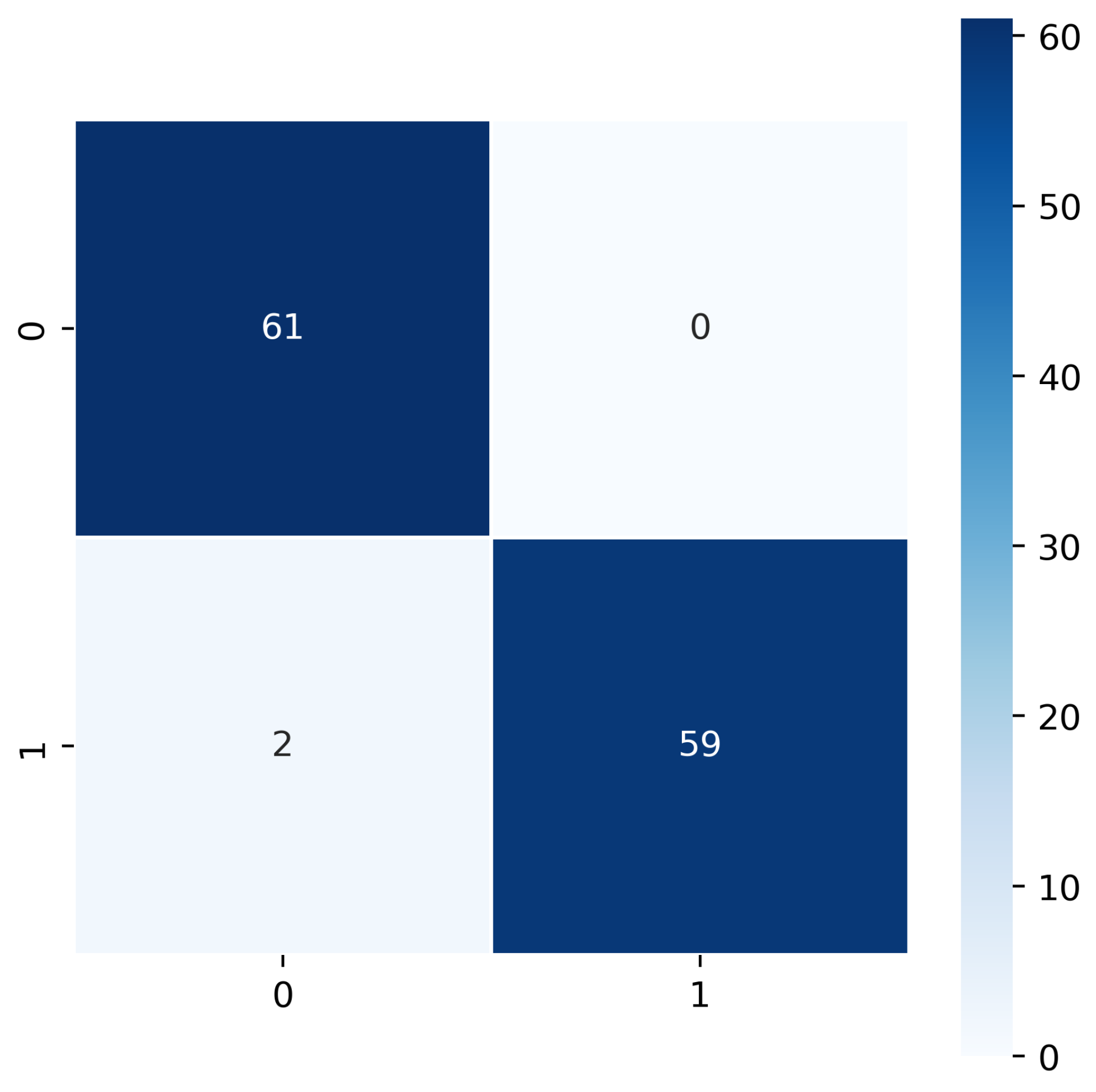
| Performance Metrics | Results (%) | Performance Metrics | Results (%) |
|---|---|---|---|
| Test Accuracy | 98.00 | FPR | 3.23 |
| Sensitivity | 98.36 | FDR | 3.23 |
| Precision | 96.77 | FNR | 1.64 |
| Specificity | 96.77 | F1 Score | 97.56 |
| NPV | 98.36 | MCC | 95.13 |
| Atlas | Class | Overall Accuracy (%) | Macro Avg (%) | Weighted Avg (%) |
|---|---|---|---|---|
| CC400 | Base CNN | 95.00 | 95.00 | 95.00 |
| Quantized CNN | 96.00 | 96.00 | 96.00 | |
| Int8 Quantized CNN (Proposed) | 96.00 | 96.00 | 96.00 | |
| CC200 | Base CNN | 96.00 | 96.00 | 96.00 |
| Quantized CNN | 97.00 | 97.00 | 97.00 | |
| Int8 Quantized CNN (Proposed) | 98.00 | 98.00 | 98.00 | |
| AAL | Base CNN | 96.00 | 96.00 | 96.00 |
| Quantized CNN | 97.00 | 97.00 | 97.00 | |
| Int8 Quantized CNN (Proposed) | 97.00 | 97.00 | 97.00 | |
| Dosenbach 160 | Base CNN | 92.00 | 92.00 | 92.00 |
| Quantized CNN | 93.00 | 93.00 | 93.00 | |
| Int8 Quantized CNN (Proposed) | 93.00 | 93.00 | 93.00 |
| Performance Metrics | Results (%) | Performance Metrics | Results (%) |
|---|---|---|---|
| Test Accuracy | 98.00 | FPR | 1.64 |
| Sensitivity | 96.72 | FDR | 1.67 |
| Precision | 98.33 | FNR | 3.28 |
| Specificity | 98.36 | F1 Score | 97.52 |
| NPV | 96.77 | MCC | 95.09 |
| Atlas | Class | Overall Accuracy (%) | Macro Avg (%) | Weighted Avg (%) |
|---|---|---|---|---|
| CC400 | Base CNN | 97.00 | 97.00 | 97.00 |
| Quantized CNN | 97.00 | 97.00 | 97.00 | |
| Int8 Quantized CNN (Proposed) | 97.00 | 97.00 | 97.00 | |
| CC200 | Base CNN | 95.00 | 95.00 | 95.00 |
| Quantized CNN | 96.00 | 96.00 | 96.00 | |
| Int8 Quantized CNN (Proposed) | 98.00 | 98.00 | 98.00 | |
| AAL | Base CNN | 97.00 | 97.00 | 97.00 |
| Quantized CNN | 97.00 | 97.00 | 97.00 | |
| Int8 Quantized CNN (Proposed) | 97.00 | 97.00 | 97.00 | |
| Dosenbach160 | Base CNN | 96.00 | 96.00 | 96.00 |
| Quantized CNN | 96.00 | 96.00 | 96.00 | |
| Int8 Quantized CNN (Proposed) | 97.00 | 97.00 | 97.00 |
| Performance Metrics | Results (%) | Performance Metrics | Results (%) |
|---|---|---|---|
| Test Accuracy | 98.00 | FPR | 3.23 |
| Sensitivity | 98.36 | FDR | 3.23 |
| Precision | 96.77 | FNR | 1.64 |
| Specificity | 96.77 | F1 Score | 97.56 |
| NPV | 98.36 | MCC | 95.13 |
| Atlas | Class | Accuracy (%) | Macro Avg (%) | Weighted Avg (%) | Support (%) |
|---|---|---|---|---|---|
| CC400 | Base CNN | 95.00 | 95.00 | 95.00 | 122 |
| Quantized CNN | 96.00 | 96.00 | 96.00 | ||
| Int8 Quantized CNN (Proposed) | 97.00 | 97.00 | 97.00 | ||
| CC200 | Base CNN | 97.00 | 97.00 | 97.00 | |
| Quantized CNN | 97.00 | 97.00 | 97.00 | ||
| Int8 Quantized CNN (Proposed) | 98.00 | 98.00 | 98.00 | ||
| AAL | Base CNN | 97.00 | 97.00 | 97.00 | |
| Quantized CNN | 97.00 | 97.00 | 97.00 | ||
| Int8 Quantized CNN (Proposed) | 97.00 | 97.00 | 97.00 | ||
| Dosenbach 160 | Base CNN | 96.00 | 96.00 | 96.00 | |
| Quantized CNN | 97.00 | 97.00 | 97.00 | ||
| Int8 Quantized CNN (Proposed) | 97.00 | 97.00 | 97.00 |
| Performance Metrics | Results (%) | Performance Metrics | Results (%) |
|---|---|---|---|
| Test Accuracy | 98.00 | FPR | 0.1 |
| Sensitivity | 96.72 | FDR | 0.1 |
| Precision | 99.98 | FNR | 3.28 |
| Specificity | 99.98 | F1 Score | 98.36 |
| NPV | 96.83 | MCC | 96.67 |
| Algorithm (Atlas) | Training Time (s) | Testing Time (s) |
|---|---|---|
| Base CNN (CC200) | 75 | 15 |
| Quantized CNN (CC200) | 57 | 11 |
| Int8 Quantized CNN (CC200) | 40 | 8 |
| Base CNN (CC400) | 65 | 13 |
| Quantized CNN (CC400) | 45 | 9 |
| Int8 Quantized CNN (CC400) | 30 | 6 |
| Base CNN (AAL) | 70 | 14 |
| Quantized CNN (AAL) | 52 | 10 |
| Int8 Quantized CNN (AAL) | 35 | 7 |
| Base CNN (Dosenbach 160) | 70 | 14 |
| Quantized CNN (Dosenbach 160) | 50 | 10 |
| Int8 Quantized CNN (Dosenbach 160) | 38 | 7 |
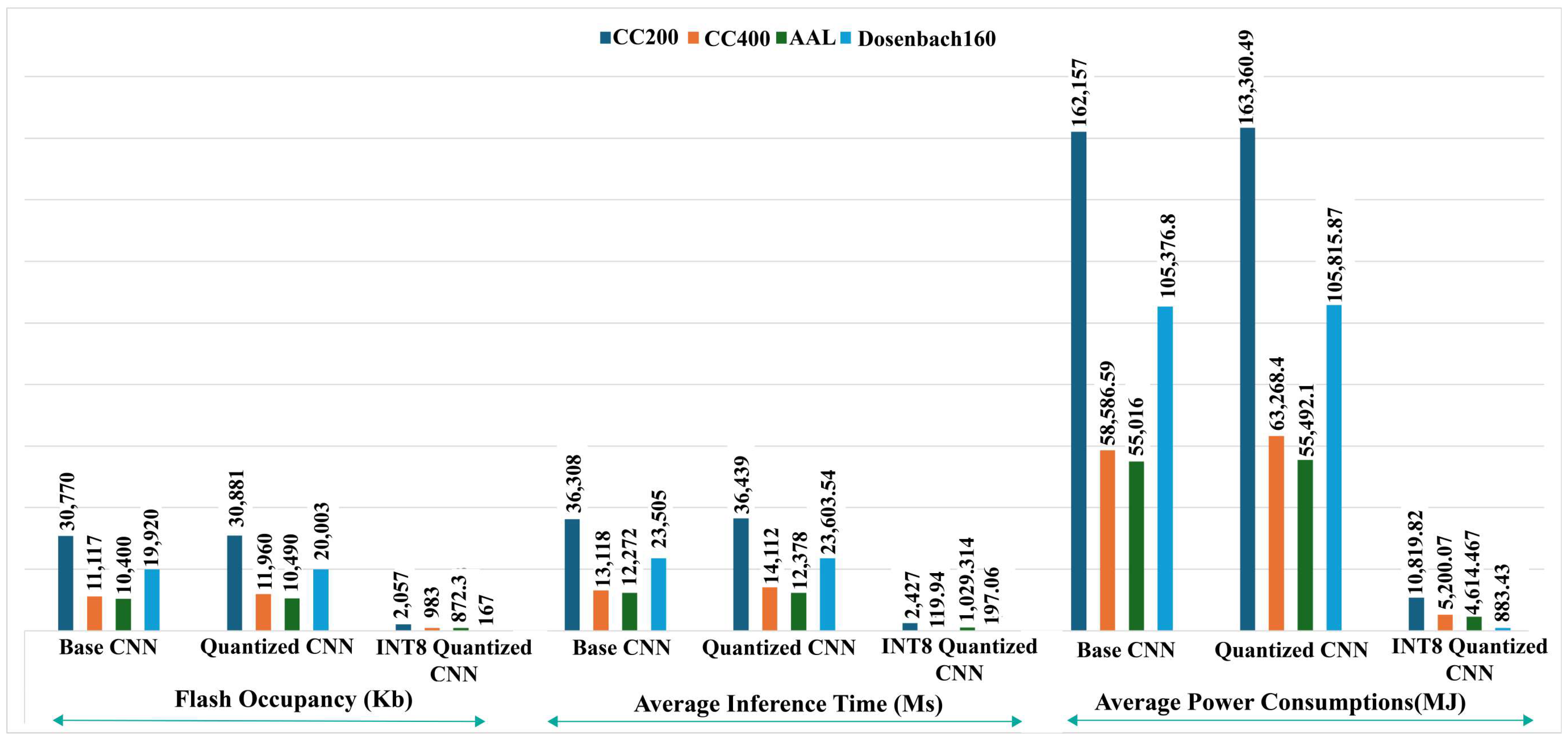
| Algorithm (Atlas) | Inference Time (ms) | Flash Occupancy (KB) | Average Power Consumption (mJ) |
|---|---|---|---|
| Base CNN (CC200) | 36,308 | 30,770 | 162,157 |
| Quantized CNN (CC200) | 36,439 | 30,881 | 163,360.49 |
| Int8 Quantized CNN (CC200) | 2427 | 2057 | 10,819.82 |
| Base CNN (CC400) | 13,118 | 11,117 | 58,586.59 |
| Quantized CNN (CC400) | 14,112 | 11,960 | 63,268.4 |
| Int8 Quantized CNN (CC400) | 119.94 | 983 | 5200.07 |
| Base CNN (AAL) | 12,272 | 10,400 | 55,016 |
| Quantized CNN (AAL) | 12,378 | 10,490 | 55,492.1 |
| Int8 Quantized CNN (AAL) | 1029.314 | 872.3 | 4614.467 |
| Base CNN (Dosenbach 160) | 23,505 | 19,920 | 105,376.8 |
| Quantized CNN (Dosenbach 160) | 23,603.54 | 20,003 | 105,815.87 |
| Int8 Quantized CNN (Dosenbach 160) | 197.06 | 167 | 883.43 |
Disclaimer/Publisher’s Note: The statements, opinions and data contained in all publications are solely those of the individual author(s) and contributor(s) and not of MDPI and/or the editor(s). MDPI and/or the editor(s) disclaim responsibility for any injury to people or property resulting from any ideas, methods, instructions or products referred to in the content. |
© 2024 by the authors. Licensee MDPI, Basel, Switzerland. This article is an open access article distributed under the terms and conditions of the Creative Commons Attribution (CC BY) license (https://creativecommons.org/licenses/by/4.0/).
Share and Cite
Gupta, S.; Bhuiyan, M.R.I.; Chowa, S.S.; Montaha, S.; Rahman, R.; Mehedi, S.T.; Rahman, Z. Enhancing Autism Spectrum Disorder Classification with Lightweight Quantized CNNs and Federated Learning on ABIDE-1 Dataset. Mathematics 2024, 12, 2886. https://doi.org/10.3390/math12182886
Gupta S, Bhuiyan MRI, Chowa SS, Montaha S, Rahman R, Mehedi ST, Rahman Z. Enhancing Autism Spectrum Disorder Classification with Lightweight Quantized CNNs and Federated Learning on ABIDE-1 Dataset. Mathematics. 2024; 12(18):2886. https://doi.org/10.3390/math12182886
Chicago/Turabian StyleGupta, Simran, Md. Rahad Islam Bhuiyan, Sadia Sultana Chowa, Sidratul Montaha, Rashik Rahman, Sk. Tanzir Mehedi, and Ziaur Rahman. 2024. "Enhancing Autism Spectrum Disorder Classification with Lightweight Quantized CNNs and Federated Learning on ABIDE-1 Dataset" Mathematics 12, no. 18: 2886. https://doi.org/10.3390/math12182886