
On Properties of the Hyperbolic Distribution

Laboratory of Control under Incomplete Information, V.A. Trapeznikov Institute of Control Sciences of RAS, Profsoyuznaya 65, 117997 Moscow, Russia
Mathematics 2024, 12(18), 2888; https://doi.org/10.3390/math12182888
Submission received: 13 August 2024
/
Revised: 10 September 2024
/
Accepted: 15 September 2024
/
Published: 16 September 2024
(This article belongs to the Section Probability and Statistics)
Abstract
:This paper is set to analytically describe properties of the hyperbolic distribution. This law, along with the variance-gamma distribution, is one of the most popular normal mean–variance mixtures from the point of view of various applications. We have found closed form expressions for the cumulative distribution and partial-moment-generating functions of the hyperbolic distribution. The obtained formulas use the values of the Humbert confluent hypergeometric and Whittaker special functions. The results are applied to the problem of European option pricing in the related Lévy model of financial market. The research demonstrates that the discussed normal mean–variance mixture is analytically tractable.
Keywords:
hyperbolic distribution; partial-moment-generating function; Humbert series; Whittaker function; digital optionMSC:
60E071. Introduction
This work continues the list of papers where the properties and applications of the hyperbolic distribution are considered. The hyperbolic distribution was introduced as a member of the family of generalized hyperbolic distributions by Barndorff-Nielsen [1]. In that paper, the hyperbolic law was suggested to be applied to the grain size analysis.
Barndorff-Nielsen [2,3] employed the hyperbolic distribution for the modeling of the turbulence effects and in statistical physics, respectively. The hyperbolic distribution was discussed in a study of the particle size distribution of sand by Barndorff-Nielsen et al. [4] and Barndorff-Nielsen and Christiansen [5]. An application of this law to the grain size analysis of coastal sediments was presented in Hartmann and Bowman [6]. To estimate the parameters of the hyperbolic distribution, Hartmann and Bowman [6] used the method of moments implemented in a special statistical program. Bhatia and Durst [7] and Xu et al. [8] used the hyperbolic distribution to model the drop size in sprays. The use of the hyperbolic law in biology was discussed in Blaesild [9]. The hyperbolic distribution was considered for the modeling of aspects of the lava magnetization by Kristjansson and McDougall [10].
Investigations in the above-mentioned areas of research based on the hyperbolic law were proceeded in more recent works. Characteristics of fluids were examined in Babinsky and Sojka [11]. Sandy systems were studied by Ghoshal et al. [12] and Hajek et al. [13]. Similarly to Barndorff-Nielsen [1], the estimation of the parameters of the hyperbolic law was made in Hajek et al. [13], applying the likeness function instead of the likelihood one. A part of modern scientific literature relates to the applications of the hyperbolic distribution to the stochastic modeling of financial market data.
It was shown that the hyperbolic distribution fits well to the empirical distributions of stock returns first by Eberlein and Keller [14]. The authors focused on the shares of the Frankfurt Stock Exchange. To assess the parameters of the hyperbolic distribution, Eberlein and Keller [14] employed maximum likelihood estimation. Bibby and Sørensen [15] used the hyperbolic law to model the volatility of the stocks of Danish companies. Eberlein et al. [16] affirmed that the hyperbolic distribution approximates the US stock market data quite well, including the NYSE composite. Proceeding the research of Eberlein and Keller [14], Küchler et al. [17] confirmed that the hyperbolic distribution satisfactorily describes not only the DAX, but also the FAZ index. To fit the parameters of the hyperbolic law, Küchler et al. [17] applied a procedure of minimizing the Kullback–Leibler distance between the probability distribution and the observed frequencies over intervals. Bauer [18] successfully tested the hyperbolic model using the data of German stocks, Dow Jones, and Nikkei indices. Daskalaki and Katris [19] showed that the hyperbolic law distinguishes well the dynamics of the CSE financial index. They provided maximum likelihood estimates of the parameters using an iterative algorithm. Calibrating portfolios of the US stock indices with multidimensional models, Luciano et al. [20] found that the hyperbolic model fits very well with both the marginal distributions and long–short investment strategies. The marginal return parameters were calibrated in Luciano et al. [20] by maximum likelihood estimation. The correlation coefficients in the multivariate case were assessed by minimizing the Frobenius distance between model and empirical correlations. It was shown in Baciu [21] that the hyperbolic distribution is very close to the empirical one in the central part for the index of the Romanian market. Cryptocurrency returns were modeled with the hyperbolic law by Sheraz and Dedu [22].
Mathematically, the hyperbolic distribution was defined in Barndorff-Nielsen [1] as the normal mean–variance mixture with the hyperbolic inverse Gaussian mixing distribution. Primary properties of the hyperbolic distribution were summarized in Barndorff-Nielsen [1] and Blaesild [23]. The Lévy measure of hyperbolic distribution was found by Eberlein and Keller [14]. The absolute moments were derived in Barndorff-Nielsen and Stelzer [24]. Special statistical techniques based on the hyperbolic law were developed in Leobacher and Pillichshammer [25] and Fonseca et al. [26]. Specifically, Fonseca et al. [26] compared the Bayesian and maximum likelihood estimators in the hyperbolic model. Following the objectives of the financial modeling including the option pricing, Eberlein and Keller [14] and Bingham and Kiesel [27] discussed the equivalent martingale change of measure for the exponent of hyperbolic distribution. Eberlein et al. [16] and Bauer [18] estimated the value at risk in the hyperbolic model. The employment of the hyperbolic law to the pension fund assessment was considered by Kabašinskas et al. [28]. An extension of the hyperbolic inverse Gaussian distribution which does not belong to the family of generalized inverse Gaussian distributions was discussed in Tan et al. [29].
As analytic representations for the cumulative distribution function, partial moments and partial-moment-generating functions of the hyperbolic distribution are not known; the computations in the hyperbolic model have to be elaborated using the Fourier transform method (Eberlein [30]) or employing a suitable simulation algorithm (Ch. XII of Asmussen and Glynn [31]). But if a distribution is considered as the substitution for the normal one in stochastic modeling, then it is desirable to describe the characteristics of this distribution in closed forms as it is made for the Gaussian one. In this paper, we obtain analytic expressions for the cumulative distribution and partial-moment-generating functions of the hyperbolic distribution. The established formulas afford to obtain in a closed form the price of the European call option.
The rest of the paper is organized as follows. Section 2 recalls the properties of hyperbolic law which are useful in the research. Section 3 formulates the main results of the work. Applications to the option pricing are given in Section 4. Section 5 numerically analyzes the difference between the normal and hyperbolic models. The method of proofs develops the ideas of Madan et al. [32], Ano and Ivanov [33], and Ivanov [34]. Detailed proofs are placed in Appendix A and Appendix B.
2. Materials and Methods
In this section, we confirm that the hyperbolic distribution can be defined as the normal mean–variance mixture where the mixing density has the hyperbolic inverse Gaussian distribution. Then, we recall the formulas for the probability density and moment-generating functions of the hyperbolic law.
2.1. Hyperbolic Inverse Gaussian Distribution
According to Eberlein and Keller [14] or Barndorff-Nielsen et al. [35], the hyperbolic inverse Gaussian distribution has two parameters and the probability density function
with
where is the modified Bessel function of the second kind.
Next, formula 3.471.9 of Gradshteyn and Ryzhik [36] includes the identity
for and . It is easy to find from (3) that the th moment of the HIG distribution for is
Once again, applying (3), one can find that the characteristic function of the HIG distribution is
If , then the moment-generating function of the HIG law exists and
2.2. Hyperbolic Distribution
2.2.1. Definition and Moments
The hyperbolic distribution is defined (see Eberlein and Keller [14] or Ch. III.1d of Shiryaev [37]) as
where , are constants, is the standard normal distribution, and is the hyperbolic inverse Gaussian distribution with the density (1) independent with the normal one. Both distributions are assumed to be defined at a probability space .
Employing the binomial expansion two times, we obtain that the moments of the hyperbolic distribution for are
where denotes the integer part of , is the double factorial of , and are the binomial coefficients.
2.2.2. Probability Density Function
2.2.3. Moment-Generating Function
So far as the characteristic function of the hyperbolic distribution
and
we find that
in accordance with (3). The moment-generating function of H exists if
Therefore, we note that
if
3. Results
Throughout this section, we introduce the analytical formulas for the cumulative distribution and partial-moment-generating functions of the hyperbolic distribution. To formulate the results, we need to enter extra constants and functions.
Let us set
and define for the function
where is the Whittaker function (see Ch. XVI of Whittaker and Watson [38]). Furthermore, let
for , where is the Humbert confluent hypergeometric series in two variables. It is defined for as the sum (see (16) in Section 1.3 of Srivastava and Karlsson [39])
where , is the Pochhammer’s symbol. The Humbert confluent hypergeometric function can be established for other values of by an analytic continuation (see Section 5.11 of Bateman and Erdélyi [40]).
The results of the paper are provided in the terms of the auxiliary functions and .
Theorem 1.
The cumulative distribution function of the hyperbolic distribution for and is computed by the identity
with
Proof Sketch.
The proof consists of four stages.
Stage 1. We pass to the computation of the integral
for , and defined in (12).
Stage 2. The integral (16) is calculated for using the Whittaker function.
Stage 3. The integral (16) is computed for employing the result of Stage 2 and leveraging the Humbert series.
The complete proof of Theorem 1 can be found in Appendix A. The next remark supplements the result of Theorem 1. We have a twin formula for and .
Remark 1.
Since
we see from Theorem 1 the similar result for and . Indeed, let , , , and , where
We have that since and as . Therefore, the conditions of Theorem 1 are satisfied for and we have that
with
Onwards, we consider the partial (or truncated) moment-generating functions of the hyperbolic distribution. The lower and upper partial-moment-generating functions of are defined as
respectively, for . The corollary below gives us a formula for the lower partial-moment-generating function of the hyperbolic distribution under the assumption that the moment-generating function of exists.
Corollary 1.
Let
Then, the lower partial-moment-generating function is determined for by the equality
where
A proof of Corollary 1 is placed in Appendix A. Same as it is got for the cumulative distribution function, we have here a cognate result for and .
Remark 2.
Summarizing, we deduce that the cumulative distribution function of the hyperbolic law is computed either if and or when and . Its partial-moment-generating functions are found either if and or when and .
4. Applications
We discuss here the traditional stochastic model of financial markets with an underlying security with price dynamics and a saving account with the evolution process (see Ch. VII.1–2 of Shiryaev [37] and Section 1.8 of Musiela and Rutkowski [41]). It is assumed that
with some constants and .
Let be the Lévy process generated by the hyperbolic distribution , that is
This process exists since has an infinitely divisible distribution, see for details Section 4 of Eberlein and Keller [14] and Ch. III.1 of Shiryaev [37]. Following, in particular, Section 3 of Carr et al. [42], we define the risk-neutral security price process as
Since is a process with independent increments, the discounted price process is a martingale with respect to the measure . Indeed, it is enough to verify the property
in this case. We have from (19) that
if . Let us notice that one may pass to the process (19) from the historical stock price applying the Esscher equivalent martingale change of measure (Eberlein et al. [43]).
Throughout this section, we discuss cash-or-nothing and asset-or-nothing digital options at time intervals . For the terminology, we refer to Section 6.5 of Musiela and Rutkowski [41]. The cash-or-nothing and asset-or-nothing digital call options have the payoffs at expiry
respectively. So far as the initial probability measure is martingale, these options have the risk-neutral prices
If , then the price of the European call option
The corollary below computes the prices of the digital options in accordance with the expectations (21).
Corollary 2.
Assume that . Then the cash-or-nothing digital call price
if and the asset-or-nothing digital call price
when .
A proof of Corollary 2 is set in Appendix B. To calculate the prices (21) and (22), we now can use the formulas of Section 3.
5. Numerical Analysis
In this section, we compare the hyperbolic law with the Gaussian distribution which has the same mean. Section 5.1 is set to select the appropriate parameters of the hyperbolic distribution. Section 5.2 presents the computation of the hyperbolic distribution values and shows the discrepancy between the normal and hyperbolic models.
5.1. Selection of the Parameters
We consider the normal distribution with mean
where is the standard Gaussian distribution. We compare it with the hyperbolic distribution
where the hyperbolic inverse-Gaussian distribution has the parameter . So far as we want the condition
to be fulfilled, the distribution should satisfy the property
5.2. Computations
Keeping in mind the values of the parameters , , and which are found in Section 5.1, we see in the notations of Theorem 1 that
and
Next,
and
It follows from formula 4.3.24 of Erdélyi et al. [44] that
for and . Hence we have that
We find from (15) that
where the values of the functions , , and are computed by (29)–(31), respectively.
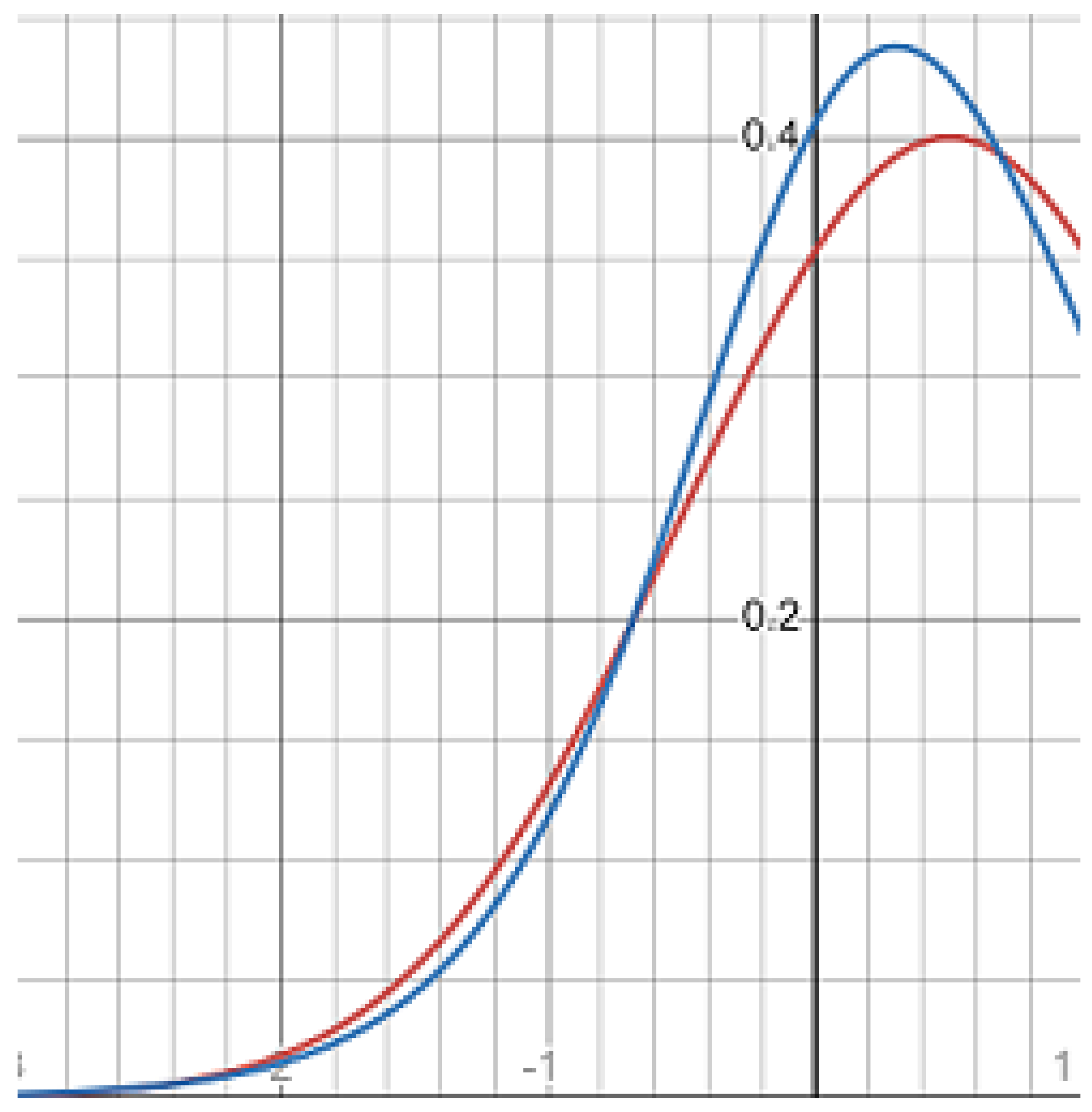
Table 1 presents the values of the cumulative distribution functions of the normal distribution (25) and the hyperbolic distribution (28). The plots of the probability density functions of the distributions at the negative axis are given at Figure 2.
To consider the difference between the normal and hyperbolic models, let us discuss the double digital option with maturity . It has two strike prices: the upper strike L and the lower strike K. The stock price becomes the exercise price if .
Let the double digital option have a cash pay . Then it has the payoffs at
and the value which is the difference between the values of two digital options. The price of this double digital option in the hyperbolic model is
Respectively, we see in the normal model that
and
Since
we have that
6. Discussion
So far as the hyperbolic distribution is widely used for the applied modeling in physics and finance, the study of its properties arises as an important scientific task. In this paper, we first find the analytical solutions for the cumulative distribution and partial-moment-generating functions of the hyperbolic distribution. The similar formulas for other normal mean–variance mixtures, including the variance-gamma distribution (Madan et al. [32], Ano and Ivanov [33], Ivanov [45]), skew Student’s t distribution (Ivanov and Temnov [46], Ivanov [47]) and semi-hyperbolic law (Ivanov [34]), depend on values of the modified Bessel function of the second kind and the Humbert confluent hypergeometric function. The obtained closed form expressions for the hyperbolic distribution use values of these two special functions as well. But in addition, they depend also on values of the Whittaker function.
The established theoretical results are applied to the problem of digital and European call option pricing in the hyperbolic Lévy model. The numerical experiments are made for the double digital options. It is shown that the risk-neutral option prices can differ at more than 12% in the hyperbolic and normal models with the same common to both models’ characteristics.
Because we have received the formulas for half of the axis, the evident proximate problem is to obtain complete analytical expressions for the cumulative distribution and partial-moment-generating functions of the hyperbolic distribution. The computation of partial moments of the hyperbolic distribution is also an actual target since it is substantial for the aim of risk measurement behind the value at risk (Cont et al. [48], Ivanov [49], Nawrocki [50]). The problem of the exotic option pricing (Ano and Ivanov [33], Section 6 of Musiela and Rutkowski [41], Schoutens et al. [51]) in the hyperbolic model should be considered as well. Taking into account the results of both this paper and Ivanov [34] for the semi-hyperbolic distribution, we may look forward for an analytical characterization of the whole subfamily with the integer second shape parameter (Perreault et al. [52]) of the family of generalized hyperbolic distributions.
7. Conclusions
Based on the discussion and results of the sections above, we can make the following conclusions.
- The hyperbolic distribution is very popular in many applications and the examination of its properties is a direction of research of current interest.
- In comparison with the formulas for other normal mean–variance mixtures, the closed form expressions for the cumulative distribution and partial-moment-generating functions of the hyperbolic law depend also on the values of the Whittaker function.
- The theoretical results can be applied to the problem of option valuation in the hyperbolic model of financial markets. It is shown that the prices of double digital options can differ by more than 12% from the prices of the same options in the normal model.
- Future investigations should relate to the complete analytical specification of the cumulative distribution, partial-moment-generating functions, and partial moments of the hyperbolic law. The research in the area of applications to finance should be continued as well.
Funding
This research received no external funding.
Data Availability Statement
Data are contained within the article.
Acknowledgments
I would like to thank the anonymous referees whose comments have significantly improved the paper.
Conflicts of Interest
The authors declare no conflicts of interest.
Appendix A
Proof of Theorem 1.
Stage 1.
Using (7), we see that the cumulative distribution function
where
with defined in (12) and
Since , we should compute the integral for . Obviously,
Set
Because of , is an increasing function of x and therefore . It follows from (A3) that x satisfies the equation
which has the solutions
so far as and .
Since , and , we see that
Therefore,
where
Onwards, we work with the integral .
We have that
with
Therefore,
where
and
Next, since
we have that
and hence .
Stage 2.
We compute at this stage the integrals and for the case .
We have that
and
Formula 3.383.3 of Gradshteyn and Ryzhik [36] contains the equality
for and . Therefore
Formula 3.383.4 of Gradshteyn and Ryzhik [36] includes the identity
for and . Hence
Stage 3.
Now we calculate and for .
Keeping in mind the case , we find that
with
and
Moreover,
with
and
It is easy to see that
and
Formula 4.3.24 of Erdélyi et al. [44] comprises the identity
for and . We have immediately from (A14) that
and
Summarizing (A4), (A6), (A12) and (A13), we obtain that
where and are computed by (A15) and (A16), respectively.
Stage 4.
Proof of Corollary 1.
Appendix B
References
- Barndorff-Nielsen, O.E. Exponentially decreasing distributions for the logarithm of particle size. Proc. R. Soc. Lond. A 1977, 353, 401–419. [Google Scholar]
- Barndorff-Nielsen, O.E. Models for non-Gaussian variation with applications to turbulence. Proc. R. Soc. Lond. A 1979, 368, 501–520. [Google Scholar]
- Barndorff-Nielsen, O.E. The hyperbolic distribution in statistical physics. Scand. J. Stat. 1982, 9, 43–46. [Google Scholar]
- Barndorff-Nielsen, O.E.; Blaesild, P.; Jensen, J.L.; Sørensen, M. The fascination of sand. In A Celebration of Statistics—The ISI Centenary Volume; Atkinson, A.C., Fienberg, S.E., Eds.; Springer: New York, NY, USA, 1985; pp. 57–87. [Google Scholar]
- Barndorff-Nielsen, O.E.; Christiansen, C. Erosion, deposition and size distribution of sand. Proc. R. Soc. Lond. A 1988, 417, 335–352. [Google Scholar]
- Hartmann, D.; Bowman, D. Efficiency of the log-hyperbolic distribution—A case study: Pattern of sediment sorting in a small tidal-inlet—Het Zwin, The Netherlands. J. Coastal Res. 1993, 9, 1044–1053. [Google Scholar]
- Bhatia, J.C.; Durst, F. Description of sprays using joint hyperbolic distribution in particle size and velocity. Combust. Flame 1990, 81, 203–218. [Google Scholar] [CrossRef]
- Xu, T.H.; Durst, F.; Tropea, C. The three-parameter log-hyperbolic distribution and its application to particle sizing. At. Sprays 1993, 3, 109–124. [Google Scholar] [CrossRef]
- Blaesild, P. On the two-dimensional hyperbolic distribution and some related distributions, with an application to Johannsen’s bean data. Biometrika 1981, 68, 251–263. [Google Scholar] [CrossRef]
- Kristjansson, L.; McDougall, I. Some aspects of the late tertiary geomagnetic field in Iceland. Geophys. J. R. Astronom. Soc. 1982, 68, 273–294. [Google Scholar] [CrossRef]
- Babinsky, E.; Sojka, P.E. Modeling drop size distributions. Prog. Energy Combust. Sci. 2002, 28, 303–329. [Google Scholar] [CrossRef]
- Ghoshal, K.; Mazumder, B.S.; Purkait, B. Grain-size distributions of bed load: Inferences from flume experiments using heterogeneous sediment beds. Sediment. Geol. 2010, 223, 1–14. [Google Scholar] [CrossRef]
- Hajek, E.A.; Huzurbazar, S.V.; Mohrig, D.; Lynds, R.M.; Heller, P.L. Statistical characterization of grain-size distributions in sandy fluvial systems. J. Sediment. Res. 2010, 80, 184–192. [Google Scholar] [CrossRef]
- Eberlein, E.; Keller, U. Hyperbolic distributions in finance. Bernoulli 1995, 1, 281–299. [Google Scholar] [CrossRef]
- Bibby, B.M.; Sørensen, M. A hyperbolic diffusion model for stock prices. Financ. Stoch. 1997, 1, 25–41. [Google Scholar] [CrossRef]
- Eberlein, E.; Keller, U.; Prause, K. New insights into smile, mispricing, and value at risk: The hyperbolic model. J. Bus. 1998, 71, 371–405. [Google Scholar] [CrossRef]
- Küchler, U.; Neumann, K.; Sørensen, M.; Streller, A. Stock returns and hyperbolic distributions. Math. Comput. Model. 1999, 29, 1–15. [Google Scholar] [CrossRef]
- Bauer, C. Value at risk using hyperbolic distributions. J. Econ. Bus. 2000, 52, 455–467. [Google Scholar] [CrossRef]
- Daskalaki, S.; Katris, C. Marginal distribution modeling and value at risk estimation for stock index returns. J. Appl. Oper. Res. 2014, 6, 207–221. [Google Scholar]
- Luciano, E.; Marena, M.; Semeraro, P. Dependence calibration and portfolio fit with factor-based subordinators. Quant. Financ. 2016, 16, 1037–1052. [Google Scholar] [CrossRef]
- Baciu, O.A. Generalized hyperbolic distributions: Empirical evidence on Bucharest stock exchange. Rev. Financ. Bank. 2015, 7, 7–18. [Google Scholar]
- Sheraz, M.H.M.; Dedu, S.A. Bitcoin cash: Stochastic models of fat-tail returns and risk modeling. Econ. Comput. Econ. Cyber. Stud. and Res. 2020, 54, 43–58. [Google Scholar]
- Blaesild, P. Conditioning with conic sections in the two-dimensional normal distribution. Ann. Stat. 1979, 7, 659–670. [Google Scholar] [CrossRef]
- Barndorff-Nielsen, O.E.; Stelzer, R. Absolute moments of generalized hyperbolic distributions and approximate scaling of normal inverse Gaussian Lévy processes. Scand. J. Stat. 2005, 32, 617–637. [Google Scholar] [CrossRef]
- Leobacher, G.; Pillichshammer, F. A method for approximate inversion of the hyperbolic CDF. Computing 2002, 69, 291–303. [Google Scholar] [CrossRef]
- Fonseca, T.; Migon, H.S.; Ferreira, M.A.R. Bayesian analysis based on the Jeffreys prior for the hyperbolic distribution. Braz. J. Probab. Statist. 2012, 26, 327–343. [Google Scholar] [CrossRef]
- Bingham, N.H.; Kiesel, R. Modelling asset returns with hyperbolic distributions. In Return Distributions in Finance; Knight, J., Satchell, S., Eds.; Butterworth-Heinemann: Oxford, UK, 2001; pp. 1–20. [Google Scholar]
- Kabašinskas, A.; Šutiene, K.; Kopa, M.; Lukšys, K.; Bagdonas, K. Dominance-based decision rules for pension fund selection under different distributional assumptions. Mathematics 2020, 8, 719. [Google Scholar] [CrossRef]
- Tan, Y.F.; Ng, K.H.; Koh, Y.B.; Peiris, S. Modelling trade durations using dynamic logarithmic component ACD model with extended generalised inverse Gaussian distribution. Mathematics 2020, 10, 1621. [Google Scholar] [CrossRef]
- Eberlein, E. Fourier-based valuation methods in mathematical finance. In Quantitative Energy Finance; Benth, F., Kholodnyi, V., Laurence, P., Eds.; Springer: New York, NY, USA, 2014; pp. 85–114. [Google Scholar]
- Asmussen, S.; Glynn, P.W. Stochastic Simulation: Algorithms and Analysis; Springer: New York, NY, USA, 2007; pp. 325–349. [Google Scholar]
- Madan, D.; Carr, P.; Chang, E. The variance gamma process and option pricing. Eur. Financ. Rev. 1998, 2, 79–105. [Google Scholar] [CrossRef]
- Ano, K.; Ivanov, R.V. On exact pricing of FX options in multivariate time-changed Lévy models. Rev. Derivat. Res. 2016, 19, 201–216. [Google Scholar]
- Ivanov, R.V. The semi-hyperbolic distribution and its applications. Stats 2023, 6, 1126–1146. [Google Scholar] [CrossRef]
- Barndorff-Nielsen, O.E.; Kent, J.; Sørensen, M. Normal mean-variance mixtures and z distributions. Int. Statist. Rev. 1982, 50, 145–159. [Google Scholar] [CrossRef]
- Gradshteyn, I.S.; Ryzhik, I.M. Table of Integrals, Series and Products, 7th ed.; Academic Press: Burlington, VT, USA, 1980; pp. 347–348, 368, 925. [Google Scholar]
- Shiryaev, A.N. Essentials of Stochastic Finance; World Scientific: Singapore, 1999; pp. 189–214, 633–661. [Google Scholar]
- Whittaker, E.T.; Watson, G.N. A Course in Modern Analysis, 4th ed.; Cambridge University Press: Cambridge, UK, 1927; pp. 337–354. [Google Scholar]
- Srivastava, H.M.; Karlsson, W. Multiple Gaussian Hypergeometric Series; Ellis Horwood Limited: New York, NY, USA, 1985; pp. 22–33. [Google Scholar]
- Bateman, H.; Erdélyi, A. Higher Transcendental Functions; McGraw-Hill: New York, NY, USA, 1953; Volume I, pp. 239–242. [Google Scholar]
- Musiela, M.; Rutkowski, M. Martingale Methods in Financial Modelling, 2nd ed.; Springer: Berlin/Heidelberg, Germany, 2005; pp. 32–34, 193–216. [Google Scholar]
- Carr, P.; Geman, H.; Madan, D.; Yor, M. Self-decomposability and option pricing. Math. Financ. 2007, 17, 31–57. [Google Scholar] [CrossRef]
- Eberlein, E.; Papapantoleon, A.; Shiryaev, A.N. Esscher transform and the duality principle for multidimensional semimartingales. Ann. Appl. Probab. 2009, 19, 1944–1971. [Google Scholar] [CrossRef]
- Erdélyi, A.; Magnus, W.; Oberhettinger, F.; Tricomi, F.G. Tables of Integral Transforms; McGraw-Hill: New York, NY, USA, 1954; Volume I, p. 139. [Google Scholar]
- Ivanov, R.V. The risk measurement under the variance-gamma process with drift switching. J. Risk Financ. Manag. 2022, 15, 22. [Google Scholar] [CrossRef]
- Ivanov, R.V.; Temnov, G. Truncated moment-generating functions of the NIG process and their applications. Stochastics Dyn. 2017, 17, 1750039. [Google Scholar] [CrossRef]
- Ivanov, R.V. On the stochastic volatility in the generalized Black-Scholes-Merton model. Risks 2023, 11, 111. [Google Scholar] [CrossRef]
- Cont, R.; Deguest, R.; He, X.D. Loss-based risk measures. Stat. Risk Model. 2013, 30, 133–167. [Google Scholar] [CrossRef]
- Ivanov, R.V. On lower partial moments for the investment portfolio with variance-gamma distributed returns. Lithuan. Math. J. 2022, 62, 10–27. [Google Scholar] [CrossRef]
- Nawrocki, D. A brief history of downside risk measures. J. Investig. 1999, 8, 9–25. [Google Scholar] [CrossRef]
- Schoutens, W.; Simons, E.; Tistaert, J. Model Risk for Exotic and Moment Derivatives. In Exotic Option Pricing and Advanced Lévy Models; Kyprianou, A.E., Schoutens, W., Wilmott, P., Eds.; Wiley: Chichester, UK, 2005; pp. 67–97. [Google Scholar]
- Perreault, L.; Bobée, B.; Rasmussen, P.F. Halphen Distribution System. I: Mathematical and Statistical Properties. J. Hydrol. Eng. 1999, 4, 189–197. [Google Scholar] [CrossRef]
Figure 1.
The normal (red) and hyperbolic (blue) probability density functions.
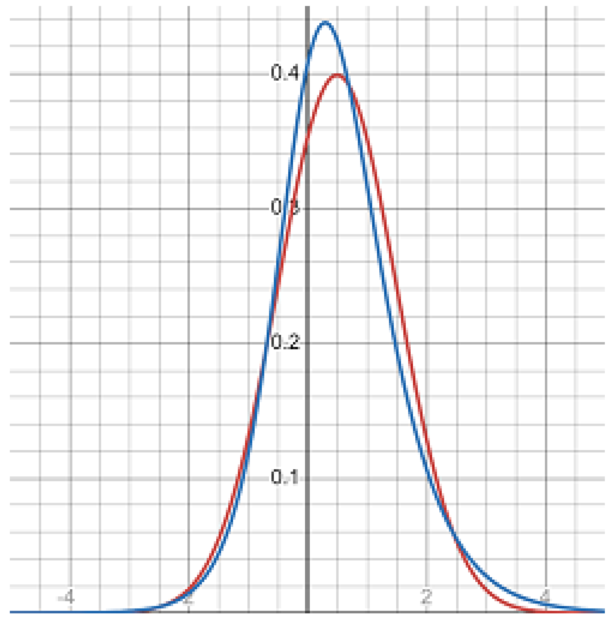
Figure 2.
The normal (red) and hyperbolic (blue) probability density functions at the negative axis.
Figure 2.
The normal (red) and hyperbolic (blue) probability density functions at the negative axis.

Table 1.
The comparison of the cumulative normal and hyperbolic distribution functions.
| u | −2 | −1 | −0.5 | −0.2 | 0 |
|---|---|---|---|---|---|
| 0.006 | 0.067 | 0.159 | 0.242 | 0.309 | |
| 0.006 | 0.058 | 0.151 | 0.241 | 0.319 |
Disclaimer/Publisher’s Note: The statements, opinions and data contained in all publications are solely those of the individual author(s) and contributor(s) and not of MDPI and/or the editor(s). MDPI and/or the editor(s) disclaim responsibility for any injury to people or property resulting from any ideas, methods, instructions or products referred to in the content. |
© 2024 by the author. Licensee MDPI, Basel, Switzerland. This article is an open access article distributed under the terms and conditions of the Creative Commons Attribution (CC BY) license (https://creativecommons.org/licenses/by/4.0/).
Share and Cite
MDPI and ACS Style
Ivanov, R.V. On Properties of the Hyperbolic Distribution. Mathematics 2024, 12, 2888. https://doi.org/10.3390/math12182888
AMA Style
Ivanov RV. On Properties of the Hyperbolic Distribution. Mathematics. 2024; 12(18):2888. https://doi.org/10.3390/math12182888
Chicago/Turabian StyleIvanov, Roman V. 2024. "On Properties of the Hyperbolic Distribution" Mathematics 12, no. 18: 2888. https://doi.org/10.3390/math12182888
Note that from the first issue of 2016, this journal uses article numbers instead of page numbers. See further details here.