Stochastic Differential Games and a Unified Forward–Backward Coupled Stochastic Partial Differential Equation with Lévy Jumps

Abstract

We establish a relationship between stochastic differential games (SDGs) and a unified forward–backward coupled stochastic partial differential equation (SPDE) with discontinuous Lévy Jumps. The SDGs have q players and are driven by a general-dimensional vector Lévy process. By establishing a vector-form Ito-Ventzell formula and a 4-tuple vector-field solution to the unified SPDE, we obtain a Pareto optimal Nash equilibrium policy process or a saddle point policy process to the SDG in a non-zero-sum or zero-sum sense. The unified SPDE is in both a general-dimensional vector form and forward–backward coupling manner. The partial differential operators in its drift, diffusion, and jump coefficients are in time-variable and position parameters over a domain. Since the unified SPDE is of general nonlinearity and a general high order, we extend our recent study from the existing Brownian motion (BM)-driven backward case to a general Lévy-driven forward–backward coupled case. In doing so, we construct a new topological space to support the proof of the existence and uniqueness of an adapted solution of the unified SPDE, which is in a 4-tuple strong sense. The construction of the topological space is through constructing a set of topological spaces associated with a set of exponents $\{{\gamma }_1,{\gamma }_2,\dots \}$ under a set of general localized conditions, which is significantly different from the construction of the single exponent case. Furthermore, due to the coupling from the forward SPDE and the involvement of the discontinuous Lévy jumps, our study is also significantly different from the BM-driven backward case. The coupling between forward and backward SPDEs essentially corresponds to the interaction between noise encoding and noise decoding in the current hot diffusion transformer model for generative AI.

1. Introduction

Recently, big data was conceptually characterized by its three-dimensional statistical features in De Mauro et al. [1]: high volume (amount of data), high velocity (speed of data in and out), and/or high variety (range of data types and sources) with respect to the movement and processing of time–space data clusters. Furthermore, Dai [2] used the general-dimensional vector Lévy process or its driven general-dimensional vector system of forward–backward coupled stochastic differential equations (FB-SDEs) to quantitatively capture the typical features of big data. Particularly, in the work of Dai [2], the Lévy jumps were used to model the instantaneous up and down movements of real-time, high-volume data clusters. From a statistical viewpoint, this process is a generalized high-dimensional Brownian motion by allowing its sample path to be discontinuous with Lévy jumps. Meanwhile, from the physical viewpoints, the Lévy jumps correspond to white non-Gaussian noises. They may be caused by random rates in semiconduct/superconduct and communication currents (see Dai [2,3] and Duncan [4] for more details), the batch arrival and processing particles in queuing systems (see, e.g., Dai and Jiang [5], Mandelbaum, and Pats [6]), and the quantum entanglement in particle systems (see, e.g., Kong et al. [7]).

More importantly, in the current and future industrial revolutions, the major concern will be about how to handle these big data optimally and fairly or how to handle them with the best efforts. Hence, based on or to build a high-performance computing or quantum-computing facility, we propose a generalized stochastic differential game (SDG) problem with Lévy jumps by unifying the concepts in Dai [3,8] and those in Karatzas and Li [9] together with artificial intelligence (AI)-aided random decision processes (i.e., AlphaGo and AlphaFold) in Silver et al. [10,11] and Jumper et al. [12], multi-game decisions in Lee et al. [13], and AI-based backward Monte Carlo simulation in Dai [14,15]. In this SDG problem, there are general q number of players with $q\in \{1,\dots ,\infty \}$. Each player $l\in \{1,\dots ,q\}$ has his own value process ${\Lambda }_l^u$ subject to a vector-form coupled FB-SDE with countable and discontinuous Lévy jumps, which is under an admissible control policy process u. The lth component $u_l(·)$ of u for each $l\in \{1,\dots ,q\}$ is the lth player’s strategy. Concerning the players’ strategies, we classify the SDG problem into two types of game problems: non-zero-sum ones and zero-sum ones.

In a non-zero-sum SDG problem (see, e.g., Dai [8], Karatzas and Li [9]), every player chooses a policy to maximize his own value process over an admissible set $\mathcal{C}$ while the summation of all the value processes is also maximized, i.e.,

$$\begin{array}{cc}& {sup}_{u\in \mathcal{C}}{\Lambda }_l^u\left(0\right)={\Lambda }_l^{u^{*}}\left(0\right)\end{array}$$

(1)

for each $l\in \{0,1,\dots ,q\}$, where

$$\begin{array}{cc}& {\Lambda }_0^u\left(t\right)={\sum }_{l=1}^q{\Lambda }_l^u\left(t\right),\end{array}$$

(2)

and ${\Lambda }_0^u\left(0\right)$ in Equation (2) does not have to be a constant (e.g., zero). In other words, all the players in this game can be in a win–win situation to share the limited resources in a communication network or a Blockchain quantum-cloud computing system. More precisely, in this game, we are interested in finding a so-called Pareto optimal Nash equilibrium policy process that is not only optimal to the whole game system but also fair to all the users.

Definition 1.

$u^{*}(·)$ is called a Nash equilibrium policy process for the non-zero-sum game in Equations (1) and (2) if no player can benefit by switching his own decision policy process unilaterally under the condition that all the others do not to change their policy processes. Mathematically, we have that

$$\begin{array}{cc}& {\Lambda }_l^{u^{*}}\left(0\right)\ge {\Lambda }_l^{u_{-l}^{*}}\left(0\right)\end{array}$$

(3)

for each $l\in \{1,\dots ,q\}$ and any given admissible control policy process u, where

$$\begin{array}{cc}& u_{-l}^{*}=(u_1^{*},\dots ,u_{l-1}^{*},u_l,u_{l+1}^{*},\dots ,u_q^{*}).\end{array}$$

Furthermore, if $u^{*}(·)$ is also an optimal one to the sum of all the q players’ value functions at time zero, i.e.,

$$\begin{array}{cc}& {\Lambda }_0^{u^{*}}\left(0\right)\ge {\Lambda }_0^u\left(0\right),\end{array}$$

(4)

it is called a Pareto optimal Nash equilibrium policy process.

However, in a zero-sum SDG problem (see, e.g., Karatzas and Li [9]), while each player chooses a policy to maximize his own value process over an admissible set $\mathcal{C}$, he also tries to minimize all the other player’s value processes, i.e.,

$$\begin{array}{ccc}& & \underset{u\in \mathcal{C}}{sup}{\Lambda }_l^u\left(0\right)={\Lambda }_l^{u^{*}}\left(0\right),\underset{u\in \mathcal{C}}{sup}(-{\Lambda }_k^u\left(0\right))=-{\Lambda }_k^{u^{*}}\left(0\right),{\Lambda }_0^u\left(0\right)=C\hfill \end{array}$$

(5)

for a constant C, a given $l\in \{1,\dots ,q\}$, and all $k\in \{1,\dots ,q\}$ with $k\ne l$.

Definition 2.

$u^{*}(·)$ is called a saddle point policy process for the zero-sum game in Equation (5) if it represents the best win to any given player l and the best efforts (i.e., the least losses) to all the other players. Mathematically, we have that

$$\begin{array}{ccc}\hfill {\Lambda }_l^{u^{*}}\left(0\right)& \ge & {\Lambda }_l^{u_{-l}^{*}}\left(0\right)for eachl\in \{1,\dots ,q\},\hfill \end{array}$$

(6)

$$\begin{array}{ccc}\hfill -{\Lambda }_k^{u^{*}}\left(0\right)& \le & -{\Lambda }_k^{u_{-k}^{*}}\left(0\right)for allk\in \{1,\dots ,q\}withk\ne l\hfill \end{array}$$

(7)

for any given admissible control policy process u, where

$$\begin{array}{ccc}\hfill u_{-l}^{*}& =& (u_1^{*},\dots ,u_{l-1}^{*},u_l,u_{l+1}^{*},\dots ,u_q^{*}),\hfill \\ \hfill u_{-k}^{*}& =& (u_1^{*},\dots ,u_{k-1}^{*},u_k,u_{k+1}^{*},\dots ,u_q^{*}).\hfill \end{array}$$

Note that in real-world applications, this type of game can be formulated to design admission control and routing policies for communication networks, power and energy grids, go games, etc. (see, e.g., Ash [16], Hamidi et al. [17], Jumper et al. [12], and Silver et al. [10,11]), with the support of high-performance quantum-cloud computing facilities (see, e.g., those proposed in Dai [8]).

The aim in studying the non-zero-sum SDG problem in Equations (1) and (2) or the zero-sum SDG problem in Equations (5) and (2) is to determine a control policy process, i.e., to determine a Pareto optimal Nash equilibrium policy process or a saddle point policy process. The key in doing so consists of two steps. The first step is to prove a vector-form It$\widehat{o}$-Ventzell formula. The second step is to prove the unique existence of the solution of a generally unified forward–backward coupled vector-form SPDE with discontinuous Lévy jumps. Here, the term SPDE is the abbreviation of stochastic partial differential equation.

If there is only one player ($q=1$) in the game, the problem in Equations (1) and (2) (or the one in Equations (5) and (2)) reduces to a conventional stochastic optimal control problem. One of the important solution methods for the SDE-based control problem is the dynamic programming. However, as pointed out in Musiela and Zariphopoulou [18], this dynamic programming method in general faces a regularity problem that is still open. Thus, Musiela and Zariphopoulou [18] derived a backward SPDE as an alternative method to solve this problem. In general, this backward SPDE is called a stochastic Hamilton–Jacobi–Bellman (HJB) equation (see, e.g., the specific backward SPDE with $q=1$ considered in Peng [19] with no jumps and Øksendal et al. [20] with Lévy jumps). However, for our proposed general SDG problem in Equations (1) and (2) (or the one in Equations (5) and (2)) with general q number of players ($q>1$), a unified system of coupled forward and backward vector-form SPDEs with Lévy jumps will be concerned. The forward SPDE is a general initial-valued one and represents the system state dynamics. The backward SPDE is a terminal-valued one (or called a Cauchy problem). Each player actually corresponds to one backward SPDE in Equation (8) as its value process in the unified vector form system. The solution of the unified system in Equation (8) corresponding to a non-zero-sum game or zero-sum game is used to derive the corresponding Nash equilibrium point policy process or saddle point policy process for each player in the multi-player game.

Hence, in this paper, we also study the existence and uniqueness of the solution of the following unified system of forward–backward coupled SPDEs with Lévy jumps along the line of our recent achievement in Dai [14,15] for a general backward SPDE driven by Brownian motion (BM). More precisely, we study the adapted 4-tuple strong solution $({\rm Y},\Lambda ,\overline{\Lambda },\tilde{\Lambda })$ to the unified system with respect to the time–position parameter $(t,x)\in R_{+}\times D$,

$$\begin{array}{c}\hfill \left\{\begin{array}{cc}{\rm Y}(t,x)\hfill & =G\left(x\right)+{\int }_0^t\mathcal{L}(s^{-},x,{\rm Y},\Lambda ,\overline{\Lambda },\tilde{\Lambda })ds\hfill \\ & +{\int }_0^t\mathcal{J}(s^{-},x,{\rm Y},\Lambda ,\overline{\Lambda },\tilde{\Lambda })dW\left(s\right)\hfill \\ & +{\int }_0^t{\int }_{{\mathcal{Z}}^h}\mathcal{I}(s^{-},x,{\rm Y},\Lambda ,\overline{\Lambda },\tilde{\Lambda },z)\tilde{N}(\lambda ds,dz),\hfill \\ \\ \Lambda (t,x)\hfill & =H\left(x\right)+{\int }_t^{\tau }\overline{\mathcal{L}}(s^{-},x,{\rm Y},\Lambda ,\overline{\Lambda },\tilde{\Lambda })ds\hfill \\ & +{\int }_t^{\tau }\overline{\mathcal{J}}(s^{-},x,{\rm Y},\Lambda ,\overline{\Lambda },\tilde{\Lambda })dW\left(s\right)\hfill \\ & +{\int }_t^{\tau }{\int }_{{\mathcal{Z}}^h}\overline{\mathcal{I}}(s^{-},x,{\rm Y},\Lambda ,\overline{\Lambda },\tilde{\Lambda },z)\tilde{N}(\lambda ds,dz),\hfill \end{array}\right.\end{array}$$

(8)

where $t\in [0,T]$, ${\mathcal{Z}}^h=R^h-\left\{0\right\}$ or $R_{+}^h$ for an integer $h>0$. Note that here, we use ${\mathcal{Z}}^h=R^h-\left\{0\right\}$ (not $R^h$) to support our Lévy measure since a Lévy measure may be singular at zero (see, e.g., Applebaum [21]). Of course, an alternative convention can also be introduced by defining a Lévy measure on $R^h$ if we assign $\nu \left(\right\{0\left\}\right)=0$ (see, e.g., Sato [22]). Furthermore, $s^{-}$ in Equation (8) denotes the corresponding left limit at time point s. In particular, $D\in R^p$ with a given $p\in \mathcal{N}=\{1,2,\dots \}$ is a connected domain, for examples, a p-dimensional box, a p-dimensional ball (or a general manifold), a p-dimensional sphere (or a general Riemannian manifold), or the whole Euclidean space $R^p$ of real numbers itself. The forward equation in Equation (8) is with the given initial random vector-field G, while the backward equation in Equation (8) has the known terminal random vector-field H. In Equation (8), ${\rm Y}$ and $\Lambda$ are r-dimensional and q-dimensional random vector-field processes, respectively. Furthermore, W denotes a standard BM that is a d-dimensional one. In addition, the notation $\tilde{N}$ denotes an h-dimensional centered Lévy jump process (or centered subordinator). More precisely, the forward equation in Equation (8) is r-dimensional, i.e., ${\rm Y}={({{\rm Y}}_1,\dots ,{{\rm Y}}_r)}^{\prime }$. Meanwhile, the backward equation in Equation (8) is q-dimensional, i.e., $\Lambda ={({\Lambda }_1,\dots ,{\Lambda }_q)}^{\prime }$. This type of vector SPDE exists in real-world applications such as color image processing and multi-mode generative AI. A color image can typically be represented by a vector PDE (see, e.g., Caselles et al. [23], Tschumperlé and Deriche [24,25,26]). In the forward image processing by noise encoding, it corresponds to a forward vector SPDE. The added noise can be a Gaussian noise or a non-Gaussian noise. In the Gaussian noise case, it corresponds to Brownian motion. In the non-Gaussion noise case, it corresponds to a Lévy process. Similarly, in the backward image processing by noise decoding for color image recovery, it corresponds to a backward vector SPDE. Furthermore, the forward image processing and backward image processing can be performed in a coupled way. In addition, the current hot area concerning multi-mode generative AI can also be explained in the same way (see, e.g., Kratsios [27], Peluchetti [28], and Vaswani et al. [29] for more details).

Concerning the explanation and importance of the 4-tuple solution $({\rm Y},\Lambda ,\overline{\Lambda },\tilde{\Lambda })$, we provide a brief introduction as follows. The random field ${\rm Y}$ described by the forward SPDE in Equation (8) corresponds to a randomized Fokker Planck equation. It is a generalized representation from a traditional mean-field game problem (see, e.g., Huang et al. [30] and Lasry and Lions [31]) to a stochastic (quantum) mean-field game (see, e.g., Kolokoltsov [32]). More precisely, ${\rm Y}$ models the observed random dynamics of particle density and distribution from a filtering system. Comparing it with the study by Kolokoltsov [32], we extend the case with Gaussian noise corresponding to the Brownian motion W in Equation (8) to the case with additional non-Gaussian noise corresponding to a pure jump Lévy process $\tilde{N}$ in Equation (8). Furthermore, we also add the feedback information $(\Lambda ,\overline{\Lambda },\tilde{\Lambda })$ from the backward SPDE in Equation (8) to the forward SPDE in Equation (8). Concerning the 3-tuple solution $(\Lambda ,\overline{\Lambda },\tilde{\Lambda })$ of the backward SPDE in Equation (8), it is a generalized situation from the case with Gaussian noise in Dai [14,15] to the case with added non-Gaussian noise. Actually, the backward SPDE in Equation (8) is a generalized Hamilton–Jacobi–Bellman (HJB) equation corresponding to a certain optimization problem, i.e.,

$$\begin{array}{c}\hfill \Lambda (t,x)=E_{Q^{*}}\left[H(T,x)|{\mathcal{F}}_t,X\left(t\right)=x\right],\end{array}$$

(9)

where $Q^{*}$ is the so-called variance optimal martingale measure (see, e.g., Dai [33]). Furthermore, ${\mathcal{F}}_t$ in Equation (9) is a sigma algebra generated by the Brownian motion and the Lévy process. Due to the martingale representation theorem for Lévy processes (see, e.g., Applebaum [21]), $\Lambda (t,x)$ can be decomposed into a macro-trend part, a Gaussian noise micro-regulating part with coefficient $\overline{\Lambda }$, and a non-Gaussian noise micro-regulating part with coefficient $\tilde{\Lambda }$. The macro-trend part may correspond to a linear or a nonlinear regression function. In the recent study of Dai [14,15], such a decomposition is referred to as a big model regression.

Note that some special form of the unified system in Equation (8) is published in Dai [14], which is a Brownian motion-driven backward SPDE subsystem of Equation (8) with useful real-world explanations. Concerning the importance and meaningfulness of the forward–backward coupled system in Equation (8), it can be explained as a generalized and randomized form of the optimality equation of the well-known mean field game problem (see, e.g., Huang et al. [30] and Lasry and Lions [31]). However, compared with the second-order partial differential operators introduced in the optimality equation of mean-field games, the orders of our partial differential operator for each $\mathcal{A}\in \{\mathcal{L},\mathcal{J},\overline{\mathcal{L}},\overline{\mathcal{J}}\}$ in Equation (8) can be a general high order. Furthermore, as mentioned previously, the coupling between the forward and backward SPDEs in Equation (8) can be used to explain the interaction between noise encoding and noise decoding in the current hot diffusion transformer model for generative AI (see, e.g., Kratsios [27], Peluchetti [28], and Vaswani et al. [29] for more details). Compared with the studies in Dai [2] and Peluchetti [28], our current SPDE-based coupling can be directly used to model the noise encoding and noise decoding interaction processes of two-dimensional plane images or images over high-dimensional manifolds (e.g., a sphere and a tori).

More precisely, the partial differential operators of r-dimensional vector $\mathcal{L}$, $r\times d$-dimensional matrix $\mathcal{J}$, and $r\times h$-dimensional matrix $\mathcal{I}$ are functionals of ${\rm Y}$, $\Lambda$, $\overline{\Lambda }$, and $\tilde{\Lambda }$, whose partial derivatives are up to the kth order for $k\in \{0,1,2,3,\dots \}$, and so are the partial differential operators of q-dimensional vector $\overline{\mathcal{L}}$, $q\times d$-dimensional matrix $\overline{\mathcal{J}}$, and $q\times h$-dimensional matrix $\overline{\mathcal{I}}$. Hereafter, for each $\mathcal{A}\in \{\mathcal{L},\mathcal{J},\overline{\mathcal{L}},\overline{\mathcal{J}}\}$, we define

$$\begin{array}{ccc}\hfill \mathcal{A}(s,x,{\rm Y},\Lambda ,\overline{\Lambda },\tilde{\Lambda },z)& \equiv & \mathcal{A}(s,x,({\rm Y},{\displaystyle \frac{\partial {\rm Y}}{\partial x_1}},\dots ,{\displaystyle \frac{{\partial }^k{\rm Y}}{\partial x_1^{i_1}\dots \partial x_p^{i_p}}})(s,x),\hfill \\ & & (\Lambda ,{\displaystyle \frac{\partial \Lambda }{\partial x_1}},\dots ,{\displaystyle \frac{{\partial }^k\Lambda }{\partial x_1^{i_1}\dots \partial x_p^{i_p}}})(s,x),\hfill \\ & & (\overline{\Lambda },{\displaystyle \frac{\partial \overline{\Lambda }}{\partial x_1}},\dots ,{\displaystyle \frac{{\partial }^k\overline{\Lambda }}{\partial x_1^{i_1}\dots \partial x_p^{i_p}}})(s,x),\hfill \\ & & (\tilde{\Lambda },{\displaystyle \frac{\partial \tilde{\Lambda }}{\partial x_1}},\dots ,{\displaystyle \frac{{\partial }^k\tilde{\Lambda }}{\partial x_1^{i_1}\dots \partial x_p^{i_p}}})(s,x,·),★),\hfill \end{array}$$

(10)

where the dot “·” in $\tilde{\Lambda }(s,x,·)$ and its associated partial derivatives denote the integration in terms of the well-known Lévy measure. Furthermore, the star “★” on the right-hand side of Equation (10) represents some stochastic factors that are supposed to be known. However, if $\mathcal{A}\in \{\mathcal{I},\overline{\mathcal{I}}\}$, the last line on the right-hand side of Equation (10) ought to be changed to an expression of the form

$$\begin{array}{ccc}& & (\tilde{\Lambda },{\displaystyle \frac{\partial \tilde{\Lambda }}{\partial x_1}},\dots ,{\displaystyle \frac{{\partial }^k\tilde{\Lambda }}{\partial x_1^{i_1}\dots \partial x_p^{i_p}}})(s,x,z),z,★.\hfill \end{array}$$

(11)

Note that our partial differential operators presented in Equation (10) can be of general nonlinearity and a general high order. For example, $\mathcal{A}$ can be taken as

$$\begin{array}{ccc}& & {\displaystyle \frac{{\partial }^k{\rm Y}}{\partial x^k}}+\lambda {\left({\displaystyle \frac{\partial {\rm Y}}{\partial x}}\right)}^k\hfill \end{array}$$

(12)

for $k\in \{1,2,3,\dots \}$ in a single-dimensional position parameter state space.

Note that if k in Equation (12) equals 2, the associated operator corresponds to the well-known KPZ equation in Hairer [34] and Kardar et al. [35]. By Cole-Hopf transformation and Itô’s formula, a solution to an SPDE associated with a scaled constant can be determined. Then, by letting the scaling factor tend to zero, a solution to the KPZ equation can be constructed and described by rough path theory. However, in our current study, we aim to show the existence and uniqueness of a solution of the generally unified system of the coupled SPDEs in Equation (8). Thus, we have different study purposes between the work in Hairer [34] and our current one. More precisely, since our unified vector-form system in Equation (8) is of a general vector dimension, general nonlinearity, general orders of partial differential operators, and general discontinuous Lévy jumps, the conventional calculation (i.e., integral by parts)-based proving approach can not be applied. Thus, by generalizing the recent study in Dai [14] from the existing Brownian motion (BM)-driven backward case to a general Lévy-driven forward–backward coupled case, we can prove the existence and uniqueness of an adapted 4-tuple strong solution to the system in Equation (8). In doing so, we construct a new topological space to support the proof. The construction of the topological space is through constructing a set of topological spaces associated with a set of exponents $\{{\gamma }_1,{\gamma }_2,\dots \}$ under a set of general local linear growth and Lipschitz conditions, which is significantly different from the construction of the single exponent case (see, e.g., Zhou and Yong [36]). Furthermore, due to the coupling from the forward SPDE and the involvement of the discontinuous Lévy jumps, our study is also significantly different from the BM-driven backward case as studied in Dai [14].

The comparison between our current work and our previous work published in Dai [14] can be summarized as follows. Our previously published work is on a sole BM-driven backward SPDE while our current work is on a generalized Lévy process-driven forward and backward coupled SPDE system. In our BM-driven backward case, the solution is a 2-tuple vector one. Meanwhile, in our current Lévy process-driven forward and backward coupled case, our solution is a 4-tuple vector one. The major difference between BM and Lévy a process is as follows: the sample path of BM is almost surely continuous while the sample path of a Lévy process can have at most countable discontinuous jump points. Furthermore, the jump size distribution needs to be controlled by an associated Lévy measure. Thus, a Lévy process is much more complicated than BM. In this sense, our Lévy process-driven SPDE is also much more complicated than a BM-driven SPDE. Since our current study is based on the forward and backward coupling, our current study has additional complexity concerning integrating the dynamics of the forward SPDE into the dynamics of the backward SPDE. Furthermore, the mentioned complexities make our newly constructed supporting topological space significantly different from the one in our previous study in Dai [14]. In addition, these complexities also make our other related discussions significantly different from those in our previous study in Dai [14].

The solution of the FB-SPDE in Equation (8) can be interpreted in a sample surface manner with a time–position parameter $(t,x)$ (for example, $\Lambda (t,x)$ can be roughly illustrated in Figure 1). Note that, the sample surfaces may involve jumps in a time parameter t since the system is driven by the Lévy type of noises.

Besides the applications in the SDG problems, our unified system of SPDEs also has importance in many other real-world systems. Interested readers are referred to the existing literature (see, e.g., Caselles et al. [23], Bouard and Debussche [37,38], Chai [39,40], Chang et al. [41], Dai [14,15,33,42], Hall [43], Karplus and Luttinger [44], Lions and Souganidis [45], Musiela and Zariphopoulou [18], Øksendal et al. [20], and Thouless [46]) for more details. In this regard, the initial random vector-field G, the terminal random vector-field H, and the 4-tuple solution process $({\rm Y},\Lambda ,\overline{\Lambda },\tilde{\Lambda })$ are allowed to be complex-valued.

The rest of the paper is organized as follows. The system of FB-SDEs for our non-zero-sum or zero-sum SDG problem is introduced in Section 2. The Queuing game and Go game aided with AlphaGo or AlphaGo Zero are exactly modeled via the system. The main theorem for the SDG game and the FB-SPDEs with required conditions are presented in Section 2.2. Finally, our main Theorem is proved in Section 3 by developing related theory.

2. Main Theorem with Examples

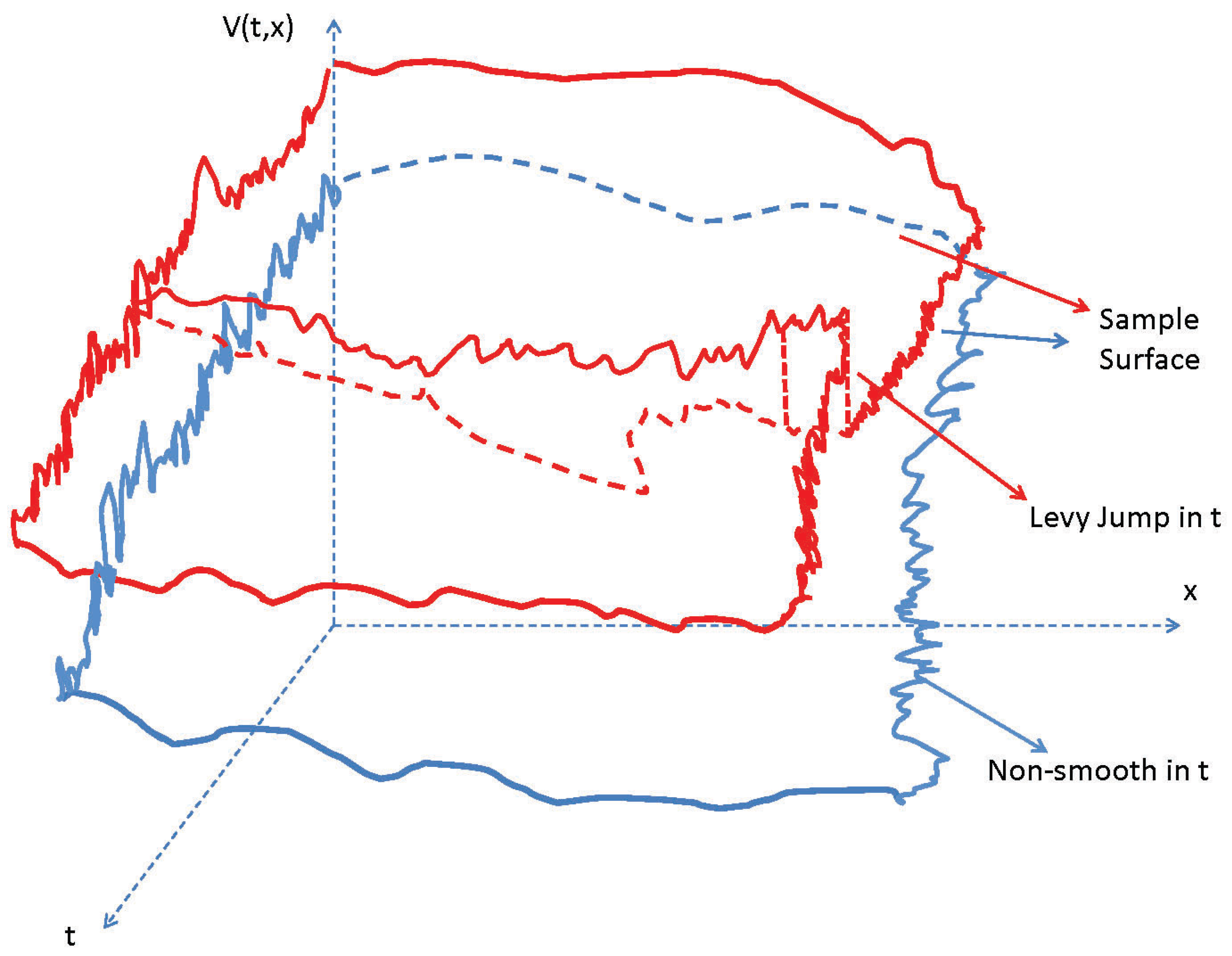
2.1. State and Value Processes

First, we consider a fixed complete probability space denoted by $(\mathsf{\Omega },\mathcal{F},P)$. On this probability space, we first define a standard d-dimensional BM $W\equiv \left\{W\right(t),t\in [0,T\left]\right\}$ with $W\left(t\right)={(W_1\left(t\right),\dots ,W_d\left(t\right))}^{\prime }$ for a given $T\in [0,\infty )$. Then, we define an h-dimensional general Lévy pure jump process $L\equiv \left\{L\right(t),t\in [0,T\left]\right\}$ with $L\left(t\right)\equiv {(L_1\left(t\right),\dots ,L_h\left(t\right))}^{\prime }$ (see, e.g., Applebaum [21], Bertoin [47], and Sato [22]). Note that the prime appearing in this paper is used to denote the associate transpose of a vector or a matrix. Moreover, we suppose that W, L, and their components are mutually independent. For a fixed $\lambda ={({\lambda }_1,\dots {\lambda }_h)}^{\prime }>0$, which is called a reversion rate vector in many applications, we let $L\left(\lambda s\right)={(L_1\left({\lambda }_{1}s\right),\dots ,L_h\left({\lambda }_{h}s\right))}^{\prime }$. Then, we denote a filtration by ${\left\{{\mathcal{F}}_t\right\}}_{t\ge 0}$ with ${\mathcal{F}}_t\equiv \sigma \{\mathcal{G},W\left(s\right),L\left(\lambda s\right):0\le s\le t\}$ for every given $t\in [0,T]$. Note that here, the notation $\mathcal{G}$ denotes a $\sigma$-algebra and is independent of W and L. In addition, we use ${\nu }_i$ for an $i\in \{1,\dots ,h\}$ to denote a Lévy measure and use $I_A(·)$ to denote the index function over a set A. Then, we can introduce the well-known Poisson random measure with a deterministic time-homogeneous intensity measure $ds{\nu }_i\left(d{z}_i\right)$ as follows:

$$\begin{array}{c}\hfill N_i((0,t]\times A)\equiv \sum _{0<s\le t}{I}_A(L_i\left(s\right)-L_i\left(s^{-}\right)).\end{array}$$

(13)

Thus, it follows from Theorem 13.4 and Corollary 13.7 in pages 237 and 239 of Kallenberg [48] that $L_i$ for each $i\in \{1,\dots ,h\}$ have the following expression:

$$\begin{array}{ccc}& & L_i\left(t\right)=a_i\left(t\right)+{\int }_{(0,t]}{\int }_{\mathcal{Z}}{z}_i{N}_i({\lambda }_{i}ds,d{z}_i),t\ge 0.\hfill \end{array}$$

(14)

For convenience, we take the constant $a_i$ to be zero.

Then, we can elaborate on the value process $V_l^u$ with $l\in \{1,\dots ,q\}$ for the non-zero-sum SDG problem in Equations (1) and (2) or the zero-sum SDG problem in Equation (5) by a generalized system of coupled FB-SDEs with Lévy jumps under a given control rule u, i.e.,

$$\begin{array}{ccc}& & \left\{\begin{array}{cc}X\left(t\right)\hfill & =x+{\int }_0^{t}b(s^{-},X,\Lambda ,\overline{\Lambda },\tilde{\Lambda },u)ds\hfill \\ & +{\int }_0^t\sigma (s^{-},X,\Lambda ,\overline{\Lambda },\tilde{\Lambda },u)dW\left(s\right)\hfill \\ & +{\int }_0^t{\int }_{{\mathcal{Z}}^h}\eta (s^{-},X,\Lambda ,\overline{\Lambda },\tilde{\Lambda },u,z)\tilde{N}(ds,dz),\hfill \\ \\ \Lambda \left(t\right)\hfill & =H(X\left(T\right),·)+{\int }_t^{T}c(s^{-},X,\Lambda ,\overline{\Lambda },\tilde{\Lambda },u)ds\hfill \\ & -{\int }_t^T\alpha (s^{-},X,\Lambda ,\overline{\Lambda },\tilde{\Lambda },u)dW\left(s\right)\hfill \\ & -{\int }_t^T{\int }_{{\mathcal{Z}}^h}\zeta (s^{-},X,\Lambda ,\overline{\Lambda },\tilde{\Lambda },u,z)\tilde{N}(ds,dz).\hfill \end{array}\right.\hfill \end{array}$$

(15)

Note that the coefficients in Equation (15) are assumed not to contain any partial derivative operators, i.e., the system in Equation (15) is the one of coupled SDEs (rather than SPDEs as in Equation (8)), and the abbreviated notion $f(t,x,X,\Lambda ,\overline{\Lambda },\tilde{\Lambda },u,z)$ for each functional $f\in \{b,\sigma ,c,\alpha ,\eta ,\zeta \}$ has the form

$$\begin{array}{c}\hfill \left\{\begin{array}{cc}f(t,X\left(t\right),\Lambda \left(t\right),\overline{\Lambda }\left(t\right),\tilde{\Lambda }(t,·),u(t,X\left(t\right)),·),\hfill & f\in \{b,\sigma ,c,\alpha \},\hfill \\ f(t,X\left(t\right),\Lambda \left(t\right),\overline{\Lambda }\left(t\right),\tilde{\Lambda }(t,z),u(t,X\left(t\right)),z,·),\hfill & f\in \{\eta ,\zeta \}.\hfill \end{array}\right.\end{array}$$

(16)

Furthermore, the proof concerning the existence and uniqueness of a solution of the system in Equations (15) and (16) is a case study for the unified FB-SDEs in Dai [2]. To be clear and to illustrate the usages of the system in Equations (15) and (16), we have the following examples.

2.2. Main Theorem

First, we present our main theorem concerning how to obtain a Pareto optimal Nash equilibrium policy process for the non-zero-sum game problem in Equations (1) and (2) subject to the constraint in Equation (15). More precisely, we define the special forms of partial differential operators $\overline{\mathcal{L}}$, $\overline{\mathcal{J}}$, and $\overline{\mathcal{I}}$ as follows, i.e., for each $l\in \{0,1,\dots ,q\}$,

$$\begin{array}{ccc}& & {\overline{\mathcal{L}}}_l(t,x,{\rm Y},\Lambda ,\overline{\Lambda },\tilde{\Lambda },u)\hfill \\ & \equiv & \sum _{i,j=1}^p{\left(\sigma {\sigma }^{\prime }\right)}_{ij}(t,x,u){\displaystyle \frac{{\partial }^2{\Lambda }_l(t,x)}{\partial x_i\partial x_j}}+\sum _{i=1}^p{b}_i(t,x,u){\displaystyle \frac{\partial {\Lambda }_l(t,x)}{\partial x_i}}\hfill \\ & & +\sum _{j=1}^d\sum _{i=1}^p{\sigma }_{ji}(t,x,u){\displaystyle \frac{\partial {\alpha }_{lj}(t,x,u)}{\partial x_i}}+c_l(t,x,u)\hfill \\ & & -\sum _{j=1}^h{\int }_{\mathcal{Z}}\left({\Lambda }_l(t,x+{\eta }_j(t,x,u,z_j))-{\Lambda }_l(t,x)-\sum _{i=1}^p{\displaystyle \frac{\partial {\Lambda }_l(t,x)}{\partial x_i}}{\eta }_{ij}(t,x,u,z_j)\right){\nu }_j\left(d{z}_j\right)\hfill \\ & & -\sum _{j=1}^h{\int }_{\mathcal{Z}}\left({\zeta }_{lj}(t,x+{\eta }_j(t,x,u,z_j),u,z_j)-{\zeta }_{lj}(t,x,u,z_j)\right){\nu }_j\left(d{z}_j\right),\hfill \end{array}$$

(17)

where ${\eta }_{ij}$ and ${\eta }_j$ for each $i\in \{1,2,\dots ,p\}$ and each $j\in \{1,2,\dots ,h\}$ are the $(i,j)$th entry and the jth column of $\eta$, respectively. Furthermore,

$$\begin{array}{ccc}\hfill c_0(t,x,u)& =& \sum _{l=1}^q{c}_l(t,x,u),\hfill \end{array}$$

(18)

$$\begin{array}{ccc}\hfill {\zeta }_{0j}(t,x,u,z_j)& =& \sum _{l=1}^q{\zeta }_{lj}(t,x,u,z_j),\hfill \end{array}$$

(19)

and ${\zeta }_{lj}$, for $l\in \{1,2,\dots ,q\}$ and $j\in \{1,2,\dots ,h\}$, is the $(i,j)$th entry of $\zeta$. Note that the partial derivative

$$\begin{array}{ccc}& & {\displaystyle \frac{\partial {\alpha }_{lj}(t,x,u)}{\partial x_i}}foreachi\in \{1,2,\dots ,p\},j\in \{1,2,\dots ,d\},andl\in \{0,1,2,\dots ,q\}\hfill \end{array}$$

should be interpreted according to chain rule since $\alpha (t,x)$ is also a function in x by $(\Lambda ,\overline{\Lambda },\tilde{\Lambda })(t,x)$ and $u(t,x)$, where

$$\begin{array}{ccc}& & {\alpha }_{0j}(t,x,u)=\sum _{l=1}^q{\alpha }_{lj}(t,x,u).\hfill \end{array}$$

(20)

Furthermore, we define

$$\begin{array}{ccc}\hfill \overline{\mathcal{J}}(t,x,{\rm Y},\Lambda ,\overline{\Lambda },\tilde{\Lambda })& =& -\overline{\Lambda }(t,x),\hfill \end{array}$$

(21)

$$\begin{array}{ccc}\hfill \overline{\mathcal{I}}(t,x,{\rm Y},\Lambda ,\overline{\Lambda },\tilde{\Lambda },z)& =& -\tilde{\Lambda }(t,x),\hfill \end{array}$$

(22)

$$\begin{array}{ccc}\hfill \Lambda (T,x)& =& H\left(x\right).\hfill \end{array}$$

(23)

Then, we have the following definitions.

Definition 3.

A set $\mathcal{C}$ of stochastic processes corresponding to the operators $\overline{\mathcal{L}}$, $\overline{\mathcal{J}}$, and $\overline{\mathcal{I}}$ in Equations (17), (21), and (22) is called the admissible set of adapted control policy processes if $\{{\overline{\mathcal{L}}}_l(t,x,{\rm Y},\Lambda$, $\overline{\Lambda },\tilde{\Lambda },u),l\in \{0,1,\dots ,q\}\}$ together with $\{\mathcal{L},\mathcal{J},\mathcal{I},\overline{\mathcal{J}},\overline{\mathcal{I}}\}$ satisfies the conditions stated in Theorem 1.

Definition 4.

$\{{\overline{\mathcal{L}}}_l(t,x,{\rm Y},\Lambda ,\overline{\Lambda },\tilde{\Lambda },u),l\in \{0,1,\dots ,q\}\}$ together with $\{\mathcal{L},\mathcal{J},\mathcal{I}\}$ is said to satisfy the comparison principle in terms of u if

$$\begin{array}{ccc}\hfill {\overline{\mathcal{L}}}_l(t,x,{{\rm Y}}^1,{\Lambda }^1,{\overline{\Lambda }}^1,{\tilde{\Lambda }}^1,u^1)& \ge & {\overline{\mathcal{L}}}_l(t,x,{{\rm Y}}^2,{\Lambda }^2,{\overline{\Lambda }}^2,{\tilde{\Lambda }}^2,u^2),\hfill \end{array}$$

(24)

$$\begin{array}{ccc}\hfill H^1\left(x\right)& \ge & H^2\left(x\right)\hfill \end{array}$$

(25)

for any $u^i\in \mathcal{C}$ and ${\mathcal{F}}_T$-measurable $H^i$ with an associated solution $({{\rm Y}}^i,{\Lambda }^i,{\overline{\Lambda }}^i,{\tilde{\Lambda }}^i)(t,x)$ of Equation (15), where $i\in \{1,2\}$ and $(t,x)\in [0,T]\times D$; then, we have

$$\begin{array}{cc}& {\Lambda }^1(t,x)\ge {\Lambda }^2(t,x).\end{array}$$

Therefore, based on these definitions, we have our main theorem for the non-zero-sum SDG problem in Equations (1) and (2) as follows.

Theorem 1.

For the operators $\{\overline{\mathcal{L}},\overline{\mathcal{J}},\overline{\mathcal{I}}\}$ in Equations (17)–(22) and under the terminal condition in Equation (23), if the $(r,q+1)$-dimensional FB-SPDEs in Equation (8) have a 4-tuple solution $({\rm Y}(t,x)$, $\Lambda (t,x)$, $\overline{\Lambda }(t,x)$, $\tilde{\Lambda }(t,x))$ and $\{{\overline{\mathcal{L}}}_l$ $(t,x,{\rm Y},\Lambda$, $\overline{\Lambda }$, $\tilde{\Lambda },u)$, $l\in \{0,1,\dots ,q\}\}$ together with $\{\mathcal{L},\mathcal{J},\mathcal{I},\overline{\mathcal{J}},\overline{\mathcal{I}}\}$ satisfies the comparison principle, there is a Pareto optimal Nash equilibrium policy process $u^{*}(t,X\left(t\right))$ over the admissible set $\mathcal{C}$ to the non-zero-sum SDG problem in Equations (1) and (2), where $\left(X\right(t)$,$\Lambda \left(t\right),\overline{\Lambda }\left(t\right),\tilde{\Lambda }(t,z))$ is the unique adapted strong solution of the FB-SDE system in Equation (15) with the coefficients $f(t,x,X,\Lambda ,\overline{\Lambda },\tilde{\Lambda },u^{*},z)$ corresponding to Equation (16) for each $f\in \{b,\sigma ,c,\alpha ,\eta ,\zeta \}$. Furthermore, the solution has the following expressions for each $j\in \{1,\dots ,h\}$:

$$\begin{array}{ccc}\hfill {\Lambda }_l\left(t\right)& =& {\Lambda }_l(t,X\left(t\right)),\hfill \end{array}$$

(26)

$$\begin{array}{ccc}\hfill {\overline{\Lambda }}_{lj}\left(t\right)& =& -\left({\alpha }_{lj}(t,X\left(t\right),u^{*})+\sum _{i=1}^p{\sigma }_{li}(t,X\left(t\right),u^{*}){\displaystyle \frac{\partial {\Lambda }_l(t,X\left(t\right))}{\partial x_i}}\right),\hfill \end{array}$$

(27)

$$\begin{array}{ccc}\hfill {\tilde{\Lambda }}_{lj}(t,z))& =& -\left({\Lambda }_l(t,X\left(t\right)+{\eta }_j(t,X\left(t\right),u^{*},z_j))-{\Lambda }_l(t,X\left(t\right))\right)\hfill \\ & & -{\zeta }_{lj}(t,X\left(t\right)+{\eta }_j(t,X\left(t\right),u^{*},z_j),u^{*},z_j).\hfill \end{array}$$

(28)

We provide a proof for Theorem 1 in Section 3. Here, we first present a counterpart for the zero-sum SDG problem in Equations (5) and (2). In this case, the system of FB-SPDEs in Equation (8) is $(r,q)$-dimensional for each $l\in \{1,\dots ,q\}$ since the terminal summation constraint should be a constant as shown in Equation (5).

Corollary 1.

For the operators $\{\overline{\mathcal{L}},\overline{\mathcal{J}},\overline{\mathcal{I}}\}$ in Equations (17)–(22) with the index l replaced by $ml$ and under the terminal condition in Equation (23), if the $(r,q^2)$-dimensional FB-SPDEs in Equation (8) have a 4-tuple solution $({\rm Y}(t,x)$, $\Lambda (t,x)$, $\overline{\Lambda }(t,x)$, $\tilde{\Lambda }(t,x))$ and $\{{\overline{\mathcal{L}}}_{ml}$ $(t,x,{\rm Y},\Lambda$,$\overline{\Lambda }$, $\tilde{\Lambda },u)$, $l\in \{1,\dots ,q\}\}$ for each $m\in \{1,\dots ,q\}$ together with $\{\mathcal{L},\mathcal{J},\mathcal{I},\overline{\mathcal{J}},\overline{\mathcal{I}}\}$ satisfies the comparison principle, there is a saddle point policy process $u^{*}(t,X\left(t\right))$ over the admissible set $\mathcal{C}$ to the zero-sum SDG problem in Equations (5) and (2) for each fixed $l\in \{1,\dots ,q\}$, where $\left(X\right(t)$,$\Lambda \left(t\right),\overline{\Lambda }\left(t\right),\tilde{\Lambda }(t,z))$ is a strong solution of the system of FB-SDEs in Equation (15). Furthermore, it is unique and adapted as given in Equations (26)–(28).

Note that the proof for Corollary 1 is similar to the one for Theorem 1. Based on Equation (5) and Definition 2, we can derive the required system of HJB equations as for Equation (17) and so on, which is a special form of FB-SPDE in Equation (8). Then, based on this system of HJB equations, we can discuss the comparison principle similar to that for Theorem 1.

2.3. Real-World Examples

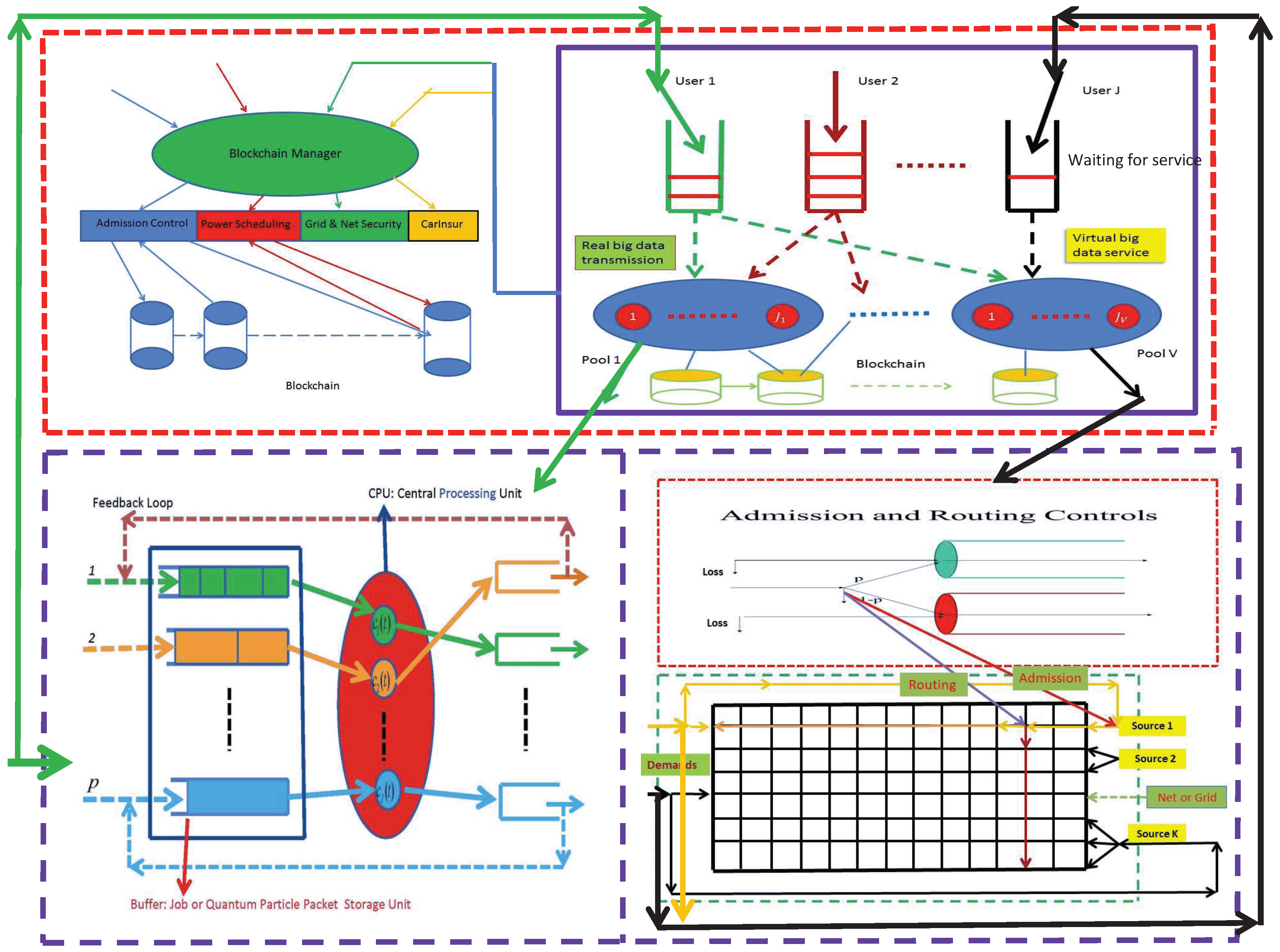
2.3.1. Sharing vs. Competition in Cloud Services and Energy Grids

In this subsubsection, we conduct case studies in terms of resources-sharing and resources-competition in quantum-cloud computing services and power-energy grids. They can be either non-zero-sum game-oriented problems or zero-sum game-oriented problems. In doing so, we use queuing networks to model the dynamics of these systems’ internal data (or more fashionably called Big Data) flows. They typically consist of arrival processes, service processes, and buffer (quantum particle) storages with a certain kind of service regime and network architecture (see, e.g., an example in Figure 2).

In this example, two real-world physical queuing systems aided with quantum-cloud computing service centers are presented. The first one in the left-lower part of Figure 2 is with p-job classes, and it can be considered as a multi-input multi-output (MIMO) wireless channel presented in Dai [3,8]. The focus of this case is on how to allocate the common shared transmission rate capacity to different users fairly in a non-zero-sum game manner. The second one in the right-lower part of Figure 2 is also with p-job classes and it typically represents a power-energy grid. In this case, the users are competing with each other in order to gain access into the grid via admission control while establishing the best routing path in a BestGo way (i.e., in a zero-sum game manner). The quantum-cloud computing service centers in the right-upper part of Figure 2 are with J-job classes. They are equipped with blockchain software architecture for the purpose of system security and management as studied in Dai [8]. Note that both the physical systems and the quantum-cloud centers can be studied as independent queuing systems. For the purpose of the current paper, we use the physical queuing systems as illustrative examples.

The major performance measure for these queuing systems is the queue length process (see, e.g., Dai [3,49]), which is represented through $Q(·)={(Q_1(·),\dots ,Q_p(·))}^{\prime }$. Each component $Q_l\left(t\right)$ denotes the number of the lth class jobs stored in the ith buffer for each $l\in \{1,\dots ,p\}$ at a fixed time point t. If we use $Q\left(0\right)$ to denote the initial queue length for the system, the queuing dynamics of these systems can be presented by

$$\begin{array}{ccc}& & Q\left(t\right)=Q\left(0\right)+A\left(t\right)-D\left(t\right),\hfill \end{array}$$

(29)

where the lth component $A_l\left(t\right)$ of $A\left(t\right)$ for each $l\in \{1,\dots ,p\}$ is the total number of jobs that arrived to buffer l by time t, and the lth component $D_l\left(t\right)$ of $D\left(t\right)$ is the total number of jobs that departed from buffer l by time t. More precisely, we assume that each $A_l(·)$ for $l\in \{1,\dots ,p\}$ is a Lévy process with intensity measure $a_l(t,Q\left(t\right),z_l)dt{\nu }_l\left(d{z}_l\right)$. In this regard, it is the job arrival rate to buffer i at time t and depends on the queue state at that moment. Furthermore, we suppose that the Lévy process is time-inhomogeneous. Similarly, we assume that each $D_i(·)$ is also a time-inhomogeneous Lévy process with intensity measure $d_l(t,Q\left(t\right),z_l)dt{\nu }_i\left(d{z}_l\right)$ that is the assigned service rate to buffer l at time t. Furthermore, we assume that the routing proportion from buffer j to buffer l for jobs finishing service at buffer j is $p_{jl}(t,Q\left(t\right),z_j)$. Based on this primitive data flow structure, we can model the dynamics that can be represented by Equation (15) for two types of typical queuing systems.

More precisely, in an inventory system (see, e.g., Dai and Jiang [5], and references therein), the queue length process $Q_l(·)$ for each $l\in \{1,\dots ,p\}$ can be either positive or negative. If $Q_l\left(t\right)\ge 0$, it is called the inventory level for the lth queue at time t, and otherwise, it is called the back-order level. Furthermore, in a general queuing system, the non-negativity of $Q_l(·)$ is usually a system constraint. However, for such a constrained dynamical system, people are frequently interested in an input and/or service fluid rate control problem; for example, the stochastic fluid limit model derived in Dai [3] has the purpose of meeting such a goal. In a fluid limit model, the impact from the constraint $Q_l(·)\ge 0$ and its associated boundary reflection is washed out owing to fluid scaling and the functional strong law of large number.

Thus, by the discussion on pages 190–193 of Applebaum [21], the queue length process in Equation (29) for an inventory system or a fluid limit model can be further expressed by a forward SDE (a special form of the forward–backward system in Equation (15)) with $\mathcal{Z}=R_{+}$, i.e.,

$$\begin{array}{ccc}\hfill d{Q}_l\left(t\right)& =& \sum _{j=1}^h{\int }_{\mathcal{Z}}{\eta }_{lj}(t,Q\left(t\right),z_j){\nu }_j\left(d{z}_j\right)dt+\sum _{j=1}^h{\int }_{\mathcal{Z}}{\eta }_{lj}(t,Q\left(t\right),z_j){\tilde{N}}_j(dt,d{z}_j),\hfill \end{array}$$

(30)

where ${\eta }_{lk}(t,Q\left(t\right),z_j)$ for each $l,k\in \{1,\dots ,p\}$ and $j\in \{1,\dots ,h\}$ is given as follows:

$$\begin{array}{ccc}& & {\eta }_{lj}(t,Q\left(t\right),z_j)=\left\{\begin{array}{cc}{a}_l(t,Q_l\left(t\right),z_l)-d_l(t,Q_l\left(t\right),z_l)\hfill & \mathrm{if}j=l,\hfill \\ \sum _{k\ne l}{p}_{kl}(t,Q_k\left(t\right),z_j)d_k(t,Q_k\left(t\right),z_j)\hfill & \mathrm{if}j\ne l.\hfill \end{array}\right.\hfill \end{array}$$

Note that the added Lévy process-driven term in Equation (30) is used to model the batch arrivals in an inventory system or the massive fluid data rate oscillation in a high-performance quantum-cloud computing based queuing system. Furthermore, the coefficients in Equation (30) may be discontinuous at the queue state $Q_l\left(t\right)=0$ for a stochastic fluid limit model. However, since the system in Equation (30) is designed in a controllable manner, the service rate $d_l(s,Q\left(s\right))$ can always be set to zero when $Q_l\left(t\right)=0$. Hence, the generalized Lipschitz and linear growth conditions required by Dai [2] may be imposed. Thus, the system in Equation (30) can still be well-posed even in this extreme case. Readers are also referred to Mandelbaum and Massey [50], Mandelbaum and Pats [6], and Konstantopoulos et al. [51] for some specific formulations of the system in Equation (30).

Next, owing to the system in Equation (30), we can formulate a queuing game problem with $q=p$. In this game, we try to schedule the service capacity over certain resource pool $\mathcal{D}$ in $R_{+}^p$ (e.g., called the available transmission rate capacity region for the related discussion in Dai [3]) in the queuing system to different players. Under a given utility function $c_l(s^{-},Q_l,{\Lambda }_l,{\overline{\Lambda }}_{l·},{\tilde{\Lambda }}_{l·})$ and a target terminal value $H_l\left(Q_l\left(T\right)\right)$, the value process for each player $l\in \{1,\dots ,p\}$ can be represented by

$$\begin{array}{ccc}\hfill {\Lambda }_l\left(t\right)& =& H_l\left(Q_l\left(T\right)\right)+{\int }_t^T{c}_l(s^{-},Q_l,{\Lambda }_l,{\overline{\Lambda }}_{l·},{\tilde{\Lambda }}_{l·})ds\hfill \\ & & -{\int }_t^T{\overline{\Lambda }}_{l·}\left(s^{-}\right)dW\left(s\right)-{\int }_t^T{\int }_{{\mathcal{Z}}^h}{\tilde{\Lambda }}_{l·}(s^{-},z)\tilde{N}(ds,dz),\hfill \end{array}$$

(31)

where ${\overline{\Lambda }}_{l·}$ and ${\tilde{\Lambda }}_{l·}$ with $l\in \{1,\dots ,p\}$ are the lth rows of $\overline{\Lambda }$ and $\tilde{\Lambda }$, respectively. Then, we first present the following claim.

Claim 2.

If $c_l(t,Q_l,{\Lambda }_l,{\overline{\Lambda }}_{l·},{\tilde{\Lambda }}_{l·})$ for each $l\in \{1,\dots ,p\}$ satisfies the generalized Lipschitz and linear growth conditions in Dai [2], there is a Pareto optimal Nash equilibrium policy for the non-zero-sum game problem in Equations (1) and (2) subject to the queuing constraint in Equation (30) and the associated value process in Equation (31).

The statement in Claim 2 is a special case of the maximum principle and our main theorem presented in Section 2.2. Note that “the generalized Lipschitz and linear growth conditions in Dai [2]” stated in Claim 2 are actually special cases of the conditions in Equations (59)–(62) in Section 3.1 of this paper. More precisely, we can present these conditions by using $f\in \{b,\sigma ,c,\alpha \}$ in Equation (15) to replace $\mathcal{A}\in \{\mathcal{L},\overline{\mathcal{L}},\mathcal{J},\overline{\mathcal{J}}\}$ in Equation (8), by using $f\in \{\eta ,\zeta \}$ in Equation (15) to replace $\mathcal{A}\in \{\mathcal{I},\overline{\mathcal{I}}\}$ in Equation (8), and by using the norm $\parallel v\parallel ={\parallel v\parallel }_{C\left(D\right)}$ without involving partial derivatives for the conditions in Dai [2] to replace the corresponding ${\parallel u\parallel }_{C^k\left(D\right)}$ involved partial derivatives in Equations (59)–(62) in the current paper. Under the generalized Lipschitz and linear growth conditions in Dai [2], the system in Equation (15) is well-posed for any measurable control function u. Thus, the state constraint for our game-theoretic problems is feasible, which means that the related Nash equilibrium point policy process and saddle point policy process may be derived.

Furthermore, here, we remark that if we consider the servers in the left-lower part of Figure 2 as input ports in a power-energy grid (e.g., the one in the right-lower part of Figure 2), different users will compete with each other to obtain the best routing path according to some routing probability (e.g., the parameter p in the right-lower part of Figure 2), some value functions (see, e.g., Dai [52]), and some routing algorithms (see, e.g., Ash [16]). On certain occasions, this type of routing problem (e.g., the well-known AlphaGo and AlphaGo Zero for mastering the Go game) may be summarized as a zero-sum game problem as formulated in Equation (5).

2.3.2. Mastering the Zero-Sum Game of Go

In a recent hot paper (i.e., Silver et al. [10,11]), the authors designed and implemented AlphaGo and AlphaGo Zero policies to master the game of Go with the help of deep neural network-based AI technologies (see, e.g., the illustration in Dai [14]). In a game of Go, two players compete with each other with the hope to surround more territory than their opponents over a grid of lines on a square board (e.g., it can be modeled as a $19\times 19$ image). More precisely, each player wishes to obtain the larger number of intersections when the rule of area scoring (i.e., a player’s score is the number of stones that the player has on the board, plus the number of empty intersections surrounded by that player’s stones) is applied. Corresponding to the dynamical representation for a queuing process in Equation (29), we use $Q_l\left(t\right)$ with $Q_l\left(0\right)=0$ for each $l\in \{1,2\}$ to denote the number of intersections won by the lth player by time t and call it the performance process for the lth player. The process $A_l\left(t\right)$ in Equation (29) with $A_l\left(0\right)=0$ is called the “win” process in this game of Go. It denotes the cumulative number of intersections won by the lth player by time t. Furthermore, it corresponds to a sequence of independently and identically distributed ($i.i.d.$) time random variables $\{{\tau }_1\left(l\right),{\tau }_2\left(l\right),\dots \}$ and a sequence of $i.i.d.$ random rewards $\{{\xi }_1\left(l\right),{\xi }_2\left(l\right),\dots \}$.

Now, consider ${\tau }_n\left(l\right)$ with ${\tau }_0\left(l\right)=0$ for each $l\in \{1,2\}$ and $n\in \{1,2,\dots \}$ as the thinking time required by the lth player to reach a decision in his nth move. In a competition of Go, the decision time is confined by some positive constant c (e.g., c takes 2 s in a competition between AlphaGo and a human expert, and meanwhile, c takes 0.2 s in a competition between AlphaGo Zero and AlphaGo). Therefore, for each $l\in \{1,2\}$, define

$$\begin{array}{c}\hfill {\tau }_n^c\left(l\right)={\tau }_n\left(l\right)I_{\{{\tau }_n\left(l\right)\le c\}},{\overline{\tau }}_n^c\left(l\right)={\tau }_n\left(l\right)I_{\{{\tau }_n\left(l\right)>c\}}\end{array}$$

(32)

and for $n\in \{0,1,\dots \}$, let

$$\begin{array}{ccc}\hfill T_0& =& 0,\hfill \end{array}$$

(33)

$$\begin{array}{ccc}\hfill T_1& =& {\tau }_1^c\left(1\right),\hfill \end{array}$$

(34)

$$\begin{array}{ccc}\hfill T_2& =& {\tau }_1^c\left(1\right)+{\tau }_1^c\left(2\right),\hfill \end{array}$$

(35)

$$\begin{array}{ccc}\hfill T_{2n+1}& =& T_{2n}+{\tau }_1^c\left(1\right),\hfill \end{array}$$

(36)

$$\begin{array}{ccc}\hfill T_{2n+2}& =& T_{2n+1}+{\tau }_1^c\left(2\right).\hfill \end{array}$$

(37)

Furthermore, let $S\left(t\right)$ denote the raw board representation of the position and its history for a game of Go at time t. In addition, let $I\left(t\right)=\{I_{[T_n,T_{n+1}]}\left(t\right),n\in \{1,2,\dots \}\}$ be the decision regime-switching indicator process, i.e., if $I\left(t\right)=I_{[T_{2n},T_{2n+1}]}\left(t\right)=1$ for some $n\in \{1,2,\dots \}$, the 1st player is in an active decision-making period while the 2nd player is in a waiting period. More precisely, at the end of each time interval $[T_{2n},T_{2n+1})$, the 1st player makes a move decision according to some probability distribution $p\left(I\right(t),S(t\left)\right)$ and a value function $v\left(I\right(t),S(t\left)\right)$ with $t=T_{2n+1}$. Note that this decision can either be made rationally by the 1st player (e.g., via AlphaGo Zero) if the thinking time ${\tau }_n\left(1\right)\le c$ or be made irrationally (say, according to a given probability distribution $p\left(1\right)$) if ${\tau }_n\left(1\right)>c$. Similarly, at the end of each interval $[T_{2n+1},T_{2n+2})$, the 2nd player makes a move decision according to some probability distribution $p\left(I\right(t),S(t\left)\right)$ and a value function $v\left(I\right(t),S(t\left)\right)$ with $t=T_{2n+2}$. This decision can also either be made rationally by the 2nd player (e.g., via AlphaGo) if the thinking time ${\tau }_n\left(2\right)\le c$ or be made irrationally (say, according to a given probability distribution $p\left(2\right)$) if ${\tau }_n\left(2\right)>c$. The main difference between AlphaGo Zero and AlphaGo is the efficiency of their internal algorithms. In a real competition, AlphaGo Zero defeated AlphaGo with scores of 100:0. Essentially, AlphaGo Zero is improved AlphaGo by the removal of the dependence of human knowledge (i.e., by removing the supervised learning of policy networks used in AlphaGo); interested readers are referred to Silver et al. [10,11] for more details. After the movement (including pass), the lth player receives a reward ${\xi }_n\left(l\right)$. It can be a value of 1 or a random number representing an area he just wins, which can be a naturally surrounding one or the one by obtained by defeating his opponent by the rule of “life” or “mutual life”. Furthermore, ${\xi }_n\left(l\right)$ can be position $S\left(t\right)$-dependent. The process $D_l\left(t\right)$ in Equation (29) with $D_l\left(0\right)=0$ is called the “loss” process in this game of Go. Besides the $i.i.d.$ random time sequence $\{{\tau }_1\left(l\right),{\tau }_2\left(l\right),\dots \}$, it is also associated with a sequence of random loss costs $\{{\zeta }_1\left(l\right),{\zeta }_2\left(l\right),\dots \}$. The cost ${\zeta }_n\left(l\right)$ for each $n\in \{1,2,\dots \}$ can be a value of zero or a random number representing the area he losses due to the rule of “death”. Moreover, ${\zeta }_n\left(l\right)$ can also be position $S\left(t\right)$-dependent.

In this study, we suppose that ${\tau }_n\left(l\right)$, for each $l\in \{1,2\}$ and $n\in \{1,2,\dots \}$, is exponentially distributed with parameter $\lambda \left(l\right)$. Let $N_l\left(t\right)$ be the total number of moves made by the lth player during time interval $[0,t]$, i.e.,

$$\begin{array}{ccc}\hfill N_1\left(t\right)& \equiv & max\left\{n,T_{2n+1}\le t\right\}\hfill \\ & =& max\left\{n,\sum _{i=1}^n{\tau }_i\left(1\right)\le t-\sum _{i=1}^{n-1}{\tau }_i^c\left(2\right)-\sum _{i=1}^n{\overline{\tau }}_i^c\left(1\right)\right\},\hfill \end{array}$$

(38)

$$\begin{array}{ccc}\hfill N_2\left(t\right)& \equiv & max\left\{n,T_{2n+2}\le t\right\}\hfill \\ & =& max\left\{n,\sum _{i=1}^n{\tau }_i^c\left(2\right)\le t-\sum _{i=1}^n{\tau }_i^c\left(1\right)-\sum _{i=1}^n{\overline{\tau }}_i^c\left(2\right)\right\}.\hfill \end{array}$$

(39)

Then, for each $l\in \{1,2\}$, the counterpart of the equation in Equation (30) can be written as

$$\begin{array}{c}\hfill Q_l\left(t\right)=\sum _{i=1}^{N_l\left(t\right)}{\xi }_i\left(l\right)-\sum _{i=1}^{N_{2-l+1}\left(t\right)}{\zeta }_i\left(l\right).\end{array}$$

(40)

By the exponential distribution assumption and the fact that the thinking times between the two players are independent, it follows from centering operations for the two terms in the right-hand side of Equation (40) that

$$\begin{array}{ccc}\hfill d{Q}_l\left(t\right)& =& {\int }_{\mathcal{Z}}{\eta }_{ll}(t,u(I\left(t\right),Q\left(t\right)),z){\nu }_l\left(dz\right)dt+{\int }_{\mathcal{Z}}{\eta }_{ll}(t,u(I\left(t\right),Q\left(t\right)),z){\tilde{N}}_l(dt,dz)\hfill \\ & & +{\int }_{\mathcal{Z}}{\eta }_{l(2-l+1)}(t,u(I\left(t\right),Q\left(t\right)),z){\nu }_{2-l+1}\left(dz\right)dt\hfill \\ & & +{\int }_{\mathcal{Z}}{\eta }_{l(2-l+1)}(t,u(I\left(t\right),Q\left(t\right)),z){\tilde{N}}_{2-l+1}(dt,dz)\hfill \end{array}$$

(41)

for each $l\in \{1,2\}$ with $\mathcal{Z}=[0,19\times 19]$. in Equation (41), ${\nu }_l\left(dz\right)$ for each $l\in \{1,2\}$ is some Lévy measure. Meanwhile, ${\tilde{N}}_l(dt,dz)$ is the corresponding compensated Poisson random measure. Since the process $Q\left(t\right)={(Q_1\left(t\right),Q_2\left(t\right))}^{\prime }$ at a time t is uniquely determined by $S\left(t\right)$, the move decision $u\left(I\right(t),Q(t\left)\right)$ in Equation (41) is given by $p\left(I\right(t),S(t\left)\right)$.

The target for a player (say, the lth player) to find such a policy is to reach the final win in this game of Go. In other words, the scores in this game competition should satisfy $Q_l\left(T\right)>Q_{2-l+1}\left(T\right)$ for each $l\in \{1,2\}$, where the notation T is the terminal time for this game. To obtain a specific representation for the value process corresponding to the one in Equation (31), we let

$$\begin{array}{ccc}\hfill H_l\left(Q\left(T\right)\right)& =& I_{\{Q_l\left(T\right)>Q_{2-l+1}\left(T\right)\}},\hfill \end{array}$$

(42)

$$\begin{array}{ccc}\hfill H\left(Q\right(T\left)\right)& =& {(H_1\left(Q\left(T\right)\right),H_2\left(Q\left(T\right)\right))}^{\prime }.\hfill \end{array}$$

(43)

Furthermore, let ${\mathcal{F}}_t=\sigma \{N_1\left(s\right),N_2\left(s\right),s\le t\}$. Then, we have that

$$\begin{array}{ccc}\hfill {\Lambda }_l\left(t\right)& =& E\left[H_l\left(Q\left(T\right)\right)|I\left(t\right),S\left(t\right)\right]\hfill \\ & =& E\left[H_l\left(Q\left(T\right)\right)|{\mathcal{F}}_t\right]\hfill \\ & =& H_l\left(Q\left(T\right)\right)-{\int }_t^T{\int }_{\mathcal{Z}}{\tilde{\Lambda }}_{l·}(s^{-},u(I\left(s\right),Q\left(s\right)),z)\tilde{N}(ds,dz),\hfill \end{array}$$

(44)

where ${\tilde{\Lambda }}_{l·}=({\tilde{\Lambda }}_{l1},{\tilde{\Lambda }}_{l2})$, $\tilde{N}(ds,dz)={({\tilde{N}}_1(ds,dz),{\tilde{N}}_2(ds,dz))}^{\prime }$. The first equality in Equation (44) is due to the definition of a Markovian decision process, and the second equality in Equation (44) is due to the martingale representation theorem (see page 266 of Applebaum [21] for more details). Thus, based on the state process in Equation (41) and the value process in Equation (44), we can formulate a zero-sum game problem as in Equation (5) for this game of Go. Furthermore, by a direct verification or by approximating through Doob’s functional representation (see, e.g., Lemma 1.13 on page 7 of Kallenberg [48]), the coefficients in Equations (41) and (44) can be assumed to satisfy the generalized Lipschitz and linear growth conditions in Dai [2]. Then, we have the following claim.

Claim 3.

Under the generalized Lipschitz and linear growth conditions in Dai [2], there is a saddle point policy process to the zero-sum game problem in Equations (5)–(2) with ${\Lambda }_1\left(0\right)+{\Lambda }_2\left(0\right)=1$ and subject to the constraints in Equations (41) and (44).

Similar to the explanation for Claim 2, Claim 3 is a special case of Corollary 1. Furthermore, “the generalized Lipschitz and linear growth conditions in Dai [2]” stated in Claim 3 can be explained in the same way as for Claim 2.

3. Proof of Main Theorem

Since the proof heavily depends on the existence and uniqueness of a solution of the $(r,q+1)$-dimensional FB-SPDEs in Equation (8), we first give a generalized discussion in Section 3.1 concerning the unified SPDE with the hope to be applied to more areas.

3.1. Unique Existence of Solution to the Unified SPDE

Let D be $R^p$ or a domain in $R^p$ and assume that there exists a sequence of nondecreasing closed and connected sets $\{D_n,n\in \mathcal{N}\}$ with $\mathcal{N}=\{0,1,\dots \}$ such that

$$\begin{array}{ccc}& & D=\bigcup _{n=0}^{\infty }{D}_n.\hfill \end{array}$$

(45)

For each $k\in \mathcal{N}$ and $l\in \{r,q\}$, let $C^k(D,R^l)$ be a Banach space endowed with the uniform norm as follows:

$$\begin{array}{ccc}& & \parallel f{\parallel }_{C^k(D,l)}^2\equiv \sum _{n=0}^{\infty }\xi (n+1)\parallel f{\parallel }_{C^k(D_n,l)}^2.\hfill \end{array}$$

(46)

Furthermore, we suppose that this Banach space consists of all continuously differentiable functions f whose derivative orders are up to the integer k. In addition, for a function $\xi \left(n\right)$ that is a discrete and fast decaying one with respect to each $n\in \{0,1,\dots \}$. More precisely, we take $\xi \left(n\right)$ as follows:

$$\begin{array}{ccc}& & \xi \left(n\right)={\displaystyle \frac{1}{(\left(n^{10}\right)!)(\eta \left(n\right)!)e^n}},\eta \left(n\right)={\left[max\left\{|x_1|+\dots +|x_p|,x\in D_n\right\}\right]}^n.\hfill \end{array}$$

(47)

Note that the notation $\left[a\right]$ used in Equation (47) denotes the summation of the unity and the integral part of number $a\in R$. Furthermore, we take

$$\begin{array}{ccc}& & \parallel f{\parallel }_{C^k(D_n,l)}=\underset{c\in \{0,1,2,\dots ,k\}}{max}\underset{j\in \{1,2,\dots ,r(c\left)\right\}}{max}\underset{x\in D_n}{sup}\left|f_j^{\left(c\right)}\left(x\right)\right|,\hfill \end{array}$$

(48)

where $r\left(c\right)$ corresponding to a $c\in \{0,1,2,\dots ,k\}$ denotes the number summation of partial derivatives whose orders are c. Furthermore, we denote

$$\begin{array}{ccc}& & f_{r,i_1\dots i_p}^{\left(c\right)}\left(x\right)={\displaystyle \frac{{\partial }^c{f}_r\left(x\right)}{\partial x_1^{i_1}\dots \partial x_p^{i_p}}}\hfill \end{array}$$

(49)

satisfying $i_1+\dots +i_p=c$ for $i_l\in \{0,1,2,\dots ,c\}$ with $l\in \{1,2,\dots ,p\}$ and $r\in \{1,2,\dots ,l\}$. Hereafter, each $j\in \{1,\dots ,r(c\left)\right\}$ is indexed in a way that it corresponds to a p-tuple $(i_1,\dots ,i_p)$ and a $r\in \{1,\dots ,l\}$, i.e.,

$$\begin{array}{ccc}\hfill f_{i_1,\dots ,i_p}^{\left(c\right)}& \equiv & (f_{1,i_1,\dots ,i_p}^{\left(c\right)},\dots ,f_{q,i_1,\dots ,i_p}^{\left(c\right)}),\hfill \end{array}$$

(50)

$$\begin{array}{ccc}\hfill f^{\left(c\right)}\left(x\right)& \equiv & (f_1^{\left(c\right)}\left(x\right),\dots ,f_{r\left(c\right)}^{\left(c\right)}\left(x\right)).\hfill \end{array}$$

(51)

Furthermore, whenever the partial derivative on the boundary $\partial D$ is concerned, it is defined in a one-side manner.

Next, let $L_{\mathcal{F}}^2([0,T],C^k(D;R^l))$ be the set consisting of $R^l$-valued random vector-field processes $Z(t,x)$. Furthermore, we suppose that these vector-field processes are measurable and adapted to the filtration $\{{\mathcal{F}}_t,t\in [0,T]\}$ corresponding to a $x\in D$. In the sequel, the “$R^l$-valued” is also called “$C^k(D;R^l)$-valued”. In this sense, the vector-field processes $Z(t,x)$ are in $C^k(D,R^l)$ for a given $t\in [0,T]$), satisfying

$$\begin{array}{ccc}& & E\left[{\int }_0^T\parallel Z\left(t\right){\parallel }_{C^k(D,l)}^{2}dt\right]<\infty .\hfill \end{array}$$

(52)

In particular, for each $l\in \{r,q\}$, let $L_{{\mathcal{G}}_l}^2(\mathsf{\Omega },C^k(D;R^l))$ be the set consisting of $R^l$-valued random vector-fields $\zeta \left(x\right)$ that are ${\mathcal{G}}_l$-measurable with each $x\in D$ and satisfy

$$\begin{array}{ccc}& & \parallel \zeta {\parallel }_{L_{\mathcal{G}}^2(\mathsf{\Omega },C^k(D,R^l))}^2\equiv E\left[\parallel \zeta {\parallel }_{C^k(D,l)}^2\right]<\infty ,\hfill \end{array}$$

(53)

where ${\mathcal{G}}_r=\mathcal{G}$ and ${\mathcal{G}}_q={\mathcal{F}}_T$. Similarly, let $L_p^2([0,T]\times {\mathcal{Z}}^h,$$C^k(D,R^{l\times h}))$ represent the set consisting of $R^{l\times h}$-valued random vector-field processes denoted by $\tilde{\Lambda }(t,x,z)=$$({\tilde{\Lambda }}_1(t,x,z_1),$$\dots ,$ ${\tilde{\Lambda }}_h(t,x,z_h))$, which are predictable for every fixed point $x\in D$ and $z\in {\mathcal{Z}}^h$ with the corresponding norm as follows:

$$\begin{array}{ccc}& & E\left[\sum _{i=1}^h{\int }_0^T{\int }_{\mathcal{Z}}{∥{\tilde{\Lambda }}_i(t,z_i)∥}_{C^k(D,l)}^2{\nu }_i\left(d{z}_i\right)dt\right]<\infty .\hfill \end{array}$$

(54)

Thus, we can define

$$\begin{array}{ccc}\hfill {\mathcal{Q}}_{\mathcal{F}}^2([0,T]\times D)& \equiv & L_{\mathcal{F}}^2([0,T],C^k(D,R^r))\hfill \\ & & \times L_{\mathcal{F}}^2([0,T],C^k(D,R^q))\hfill \\ & & \times L_{\mathcal{F},p}^2([0,T],C^k(D,R^{q\times d}))\hfill \\ & & \times L_p^2([0,T]\times {\mathcal{Z}}^h,C^k(D,R^{q\times h})).\hfill \end{array}$$

(55)

Finally, let

$$\begin{array}{ccc}& & L_{\nu }^2({\mathcal{Z}}^h,C^c(D,R^{q\times h}))\hfill \\ & & \equiv \left\{\tilde{v}:{\mathcal{Z}}^h\to C^c(D,R^{q\times h}),\sum _{i=1}^h{\int }_{\mathcal{Z}}{∥{\tilde{v}}_i\left(z_i\right)∥}_{C^c(D,q)}^2{\nu }_i\left(d{z}_i\right)<\infty \right\}\hfill \end{array}$$

(56)

which is endowed with the norm

$$\begin{array}{ccc}& & \parallel \tilde{v}{\parallel }_{D,\nu ,c}^2\equiv \sum _{i=1}^h{\int }_{\mathcal{Z}}{∥{\tilde{v}}_i\left(z_i\right)∥}_{C^c(D,q)}^2{\lambda }_i{\nu }_i\left(d{z}_i\right)\hfill \end{array}$$

(57)

for any $\tilde{v}\in L_{\nu }^2({\mathcal{Z}}^h,C^c(D,R^{q\times h}))$ and $c\in \{0,1,\dots ,k\}$. Furthermore, define

$$\begin{array}{ccc}\hfill {\mathcal{V}}^k\left(D\right)& \equiv & C^k(D,R^r)\hfill \\ & & \times C^k(D,R^q)\hfill \\ & & \times C^k(D,R^{q\times d})\hfill \\ & & \times {\overline{L}}_{\nu }^2({\mathcal{Z}}^h,C^k(D,R^{q\times h})).\hfill \end{array}$$

(58)

Then, we can impose some conditions to guarantee the existence and uniqueness of a 4-tuple solution of the unified FB-SPDE in Equation (8), which is a strong and adapted solution.

First, for each $\mathcal{A}\in \{\mathcal{L},\overline{\mathcal{L}},\mathcal{J},\overline{\mathcal{J}}\}$ and any $(u^i,v^i,{\overline{v}}^i,{\tilde{v}}^i)\in {\mathcal{V}}^k\left(D\right)$ with $i\in \{1,2\}$, we define

$$\begin{array}{ccc}& & \Delta \mathcal{A}(s,x,u^1,v^1,{\overline{v}}^1,{\tilde{v}}^1,u^2,v^2,{\overline{v}}^2,{\tilde{v}}^2)\hfill \\ & \equiv & \mathcal{A}(s,x,u^1,v^1,{\overline{v}}^1,{\tilde{v}}^1)-\mathcal{A}(s,x,u^2,v^2,{\overline{v}}^2,{\tilde{v}}^2).\hfill \end{array}$$

Then, we assume that the generalized local Lipschitz condition is true almost surely (a.s.),

$$\begin{array}{ccc}& & ∥\Delta \mathcal{A}(s,x,u^1,v^1,{\overline{v}}^1,{\tilde{v}}^1,u^2,v^2,{\overline{v}}^2,{\tilde{v}}^2)∥\hfill \\ & \le & K_{D_n}\left(\parallel u^1-u^2{\parallel }_{C^k(D_n,r)}+\parallel v^1-v^2{\parallel }_{C^k(D_n,q)}+\parallel {\overline{v}}^1-{\overline{v}}^2{\parallel }_{C^k(D_n,qd)}+{\parallel {\tilde{v}}^1-{\tilde{v}}^2\parallel }_{D_n,\nu ,k}\right),\hfill \end{array}$$

(59)

where the constant $K_{D_n}\ge 0$ depends on $D_n$ and may be unbounded as $D_n\to D$ along $n\in \{0,1,2,\dots \}$. Note that for a vector (or a matrix) A, we use $\parallel A\parallel$ to denote the largest absolute value of its components (or entries). Furthermore, for each $\mathcal{A}\in \{\mathcal{I},\overline{\mathcal{I}}\}$, we suppose that

$$\begin{array}{ccc}& & \sum _{i=1}^h{\int }_{\mathcal{Z}}{∥\Delta {\mathcal{A}}_i(s,x,u^1,v^1,{\overline{v}}^1,{\tilde{v}}^1,u^2,v^2,{\overline{v}}^2,{\tilde{v}}^2,z_i)∥}^2{\lambda }_i{\nu }_i\left(d{z}_i\right)\hfill \\ & \le & K_{D_n}\left(\parallel u^1-u^2{\parallel }_{C^k(D_n,r)}^2+\parallel v^1-v^2{\parallel }_{C^k(D_n,q)}^2+\parallel {\overline{v}}^1-{\overline{v}}^2{\parallel }_{C^k(D_n,qd)}^2+{\parallel {\tilde{v}}^1-{\tilde{v}}^2\parallel }_{D_n,\nu ,k}^2\right),\hfill \end{array}$$

(60)

where ${\mathcal{A}}_i$ is the ith column of $\mathcal{A}$.

Second, for each $\mathcal{A}\in \{\mathcal{L},\overline{\mathcal{L}},\mathcal{J},\overline{\mathcal{J}}\}$ and any $(u,v,\overline{v},\tilde{v})\in {\mathcal{V}}^k\left(D\right)$, we assume that the generalized linear growth condition holds

$$\begin{array}{ccc}& & ∥\mathcal{A}(s,x,u,v,\overline{v},\tilde{v})∥\hfill \\ & \le & K_{D_n}\left({\parallel u\parallel }_{C^k(D_n,r)}+{\parallel v\parallel }_{C^k(D_n,q)}+\parallel \overline{v}{\parallel }_{C^k(D_n,qd)}+{\parallel \tilde{v}\parallel }_{D_n,\nu ,k}\right).\hfill \end{array}$$

(61)

Similarly, for each $\mathcal{A}\in \{\mathcal{I},\overline{\mathcal{I}}\}$, we suppose that

$$\begin{array}{ccc}& & \sum _{i=1}^h{\int }_{\mathcal{Z}}{∥{\mathcal{A}}_i(s,x,u,v,\overline{v},\tilde{v},z_i)∥}^2{\lambda }_i\nu \left(d{z}_i\right)\hfill \\ & \le & K_{D_n}\left({\parallel u\parallel }_{C^k(D_n,r)}^2+{\parallel v\parallel }_{C^k(D_n,q)}^2+\parallel \overline{v}{\parallel }_{C^k(D_n,qd)}^2+{\parallel \tilde{v}\parallel }_{D_n,\nu ,k}^2\right).\hfill \end{array}$$

(62)

Concerning the reasonability of conditions in Equations (59)–(62), it can be illustrated as follows. If all the concerned partial derivative operators are linear, these conditions are naturally satisfied (see the examples in Dai [14] for numerical simulations). Even if these partial derivative operators are strongly nonlinear, we can still use some approximation techniques to make these conditions useful in some applications (see, e.g., Dai [15]).

Now, let ${\mathbb{C}}^l$ be the l-dimensional complex Euclidean space and all the related norms are interpreted in the corresponding complex-valued sense. Then, we can present a proposition as follows.

Proposition 1.

Suppose that $(G,H)\in L_{\mathcal{G}}^2(\mathsf{\Omega },C^k(D;{\mathbb{C}}^r))\times L_{{\mathcal{F}}_T}^2(\mathsf{\Omega },C^k(D;{\mathbb{C}}^q))$ and conditions in Equations (59)–(62) are true. Furthermore, assume that each $\mathcal{A}\in \{\mathcal{L},\overline{\mathcal{L}},\mathcal{J},\overline{\mathcal{J}},\mathcal{I},\overline{\mathcal{I}}\}$ is $\left\{{\mathcal{F}}_t\right\}$-adapted for every fixed $x\in D$, $z\in {\mathcal{Z}}^h$, and any given $(u,v,\overline{v},\tilde{v})\in {\mathcal{V}}^k\left(D\right)$ with

$$\begin{array}{ccc}& & \mathcal{L}(·,x,0)\in L_{\mathcal{F}}^2\left([0,T],C^k(D,{\mathbb{C}}^r)\right),\hfill \end{array}$$

(63)

$$\begin{array}{ccc}& & \mathcal{J}(·,x,0)\in L_{\mathcal{F}}^2\left([0,T],C^k(D,{\mathbb{C}}^{r\times d})\right),\hfill \end{array}$$

(64)

$$\begin{array}{ccc}& & \mathcal{I}(·,x,0,·)\in L_{\mathcal{F}}^2\left([0,T]\times {\mathcal{Z}}^h,C^k(D,{\mathbb{C}}^{r\times h})\right),\hfill \end{array}$$

(65)

$$\begin{array}{ccc}& & \overline{\mathcal{L}}(·,x,0)\in L_{\mathcal{F}}^2\left([0,T],C^k(D,{\mathbb{C}}^q)\right),\hfill \end{array}$$

(66)

$$\begin{array}{ccc}& & \overline{\mathcal{J}}(·,x,0)\in L_{\mathcal{F}}^2\left([0,T],C^k(D,{\mathbb{C}}^{q\times d})\right),\hfill \end{array}$$

(67)

$$\begin{array}{ccc}& & \overline{\mathcal{I}}(·,x,0,·)\in L_{\mathcal{F}}^2\left([0,T]\times {\mathcal{Z}}^h,C^k(D,{\mathbb{C}}^{q\times h})\right).\hfill \end{array}$$

(68)

Then, there uniquely exists a 4-tuple solution of the unified FB-SPDE in Equation (8), which is a strong and adapted solution, i.e.,

$$\begin{array}{ccc}& & ({\rm Y},\Lambda ,\overline{\Lambda },\tilde{\Lambda })\in {\mathcal{Q}}_{\mathcal{F}}^2([0,T]\times D),\hfill \end{array}$$

(69)

and $({\rm Y},\Lambda )(·,x)$ is càdlàg for each $x\in D$ almost surely (a.s.).

Note that in Proposition 1, the forward equation is r-dimensional, i.e., ${\rm Y}={({{\rm Y}}_1,\dots ,{{\rm Y}}_r)}^{\prime }$. Meanwhile, the backward equation is q-dimensional, i.e., $\Lambda ={({\Lambda }_1,\dots ,{\Lambda }_q)}^{\prime }$. This type of vector SPDE exists in real-world applications such as color image processing and multi-mode generative AI. The existence and uniqueness of such a vector solution proved in the proposition can guarantee the image processing and recovery in a multi-channel computer vision and network system. For example, a color image can typically be represented by a vector PDE (see, e.g., Caselles et al. [23], Tschumperlé and Deriche [24,25,26]). In the image forward processing by noise encoding, it corresponds to a forward vector SPDE. The added noise can be a Gaussian noise or a non-Gaussian noise. In the Gaussian noise case, it corresponds to Brownian motion. In the non-Gaussian noise case, it corresponds to a Lévy process. Similarly, in the backward image processing by noise decoding for color image recovery, it corresponds to a backward vector SPDE. Furthermore, the forward image processing and backward image processing can be in a coupled way. In addition, the current hot area concerning multi-mode generative AI can also be explained in the same way (see, e.g., Kratsios [27], Peluchetti [28], and Vaswani et al. [29] for more details) as introduced in the introduction of this paper. Finally, for the convenience of presentation, in the next subsection, we first prove our main theorem (Theorem 1) in Section 3.2 by assuming the truth of Proposition 1. Then, we prove Proposition 1 formally in Section 3.3.

3.2. Proof of Theorem 1

Proof. 

First, if the claim in Proposition 1 is true, we can prove a general q-dimensional vector-form It$\widehat{o}$-Ventzell formula with Lévy jumps. More precisely, consider the operators $\{\overline{\mathcal{L}},\overline{\mathcal{J}},\overline{\mathcal{I}}\}$ given in Proposition 1 and suppose $\Lambda (t,x)$ is a solution of the q-dimensional vector-form B-SPDE with Lévy jumps:

$$\begin{array}{ccc}\hfill d\Lambda (t,x)& =& \overline{\mathcal{L}}(t^{-},x,{\rm Y},\Lambda ,\overline{\Lambda },\tilde{\Lambda },u)dt+\overline{\mathcal{J}}(t^{-},x,{\rm Y},\Lambda ,\overline{\Lambda },\tilde{\Lambda },u)dW\left(t\right)\hfill \\ & & +{\int }_{{\mathcal{Z}}^h}\overline{\mathcal{I}}(t^{-},x,{\rm Y},\Lambda ,\overline{\Lambda },\tilde{\Lambda },u,z)\tilde{N}(\lambda dt,dz).\hfill \end{array}$$

(70)

Furthermore, assume that X is a solution of the p-dimensional vector-form F-SDE given by

$$\begin{array}{ccc}\hfill dX\left(t\right)& =& b(t^{-},X,\Lambda ,\overline{\Lambda },\tilde{\Lambda },u)dt+\sigma (t^{-},X,\Lambda ,\overline{\Lambda },\tilde{\Lambda },u)dW\left(t\right)\hfill \\ & & +{\int }_{{\mathcal{Z}}^h}\eta (t^{-},X,\Lambda ,\overline{\Lambda },\tilde{\Lambda },u,z)\tilde{N}(dt,dz).\hfill \end{array}$$

(71)

In addition, for a $t\in [0,T]$, let

$$\begin{array}{ccc}& & \Lambda \left(t\right)\equiv \Lambda (t,X(t\left)\right).\hfill \end{array}$$

(72)

Then, by applying It$\widehat{o}$’s formula presented in Theorem 1.16 of ksendal and Sulem [53], we can extend the It$\widehat{o}$-Ventzell formula with Lévy jumps in single-dimensional case (see, e.g., Øksendal and Zhang [54]) to the general q-dimensional vector-form situation as follows:

$$\begin{array}{ccc}\hfill d\Lambda \left(t\right)& =& \{\overline{\mathcal{L}}(t^{-},X)+\sum _{i=1}^p{\displaystyle \frac{\partial \Lambda (t,X(t\left)\right)}{\partial x_i}}{b}_i(t^{-},X)\hfill \\ & & +\sum _{i=1}^p{\displaystyle \frac{\partial \overline{\mathcal{J}}(t^{-},X)}{\partial x_i}}{\left({\sigma }^{\prime }(t^{-},X)\right)}_i\hfill \\ & & +{\displaystyle \frac{1}{2}}\sum _{i,j=1}^p{\displaystyle \frac{\partial {\Lambda }^2(t,X\left(t\right))}{\partial x_i\partial x_j}}{\left(\left(\sigma (t^{-},X){\sigma }^{\prime }(t^{-},X)\right)\right)}_{ij}\hfill \\ & & +\sum _{j=1}^h{\int }_{z_j\in \mathcal{Z}}(\Lambda (t^{-},X\left(t^{-}\right)+{\eta }_j(t^{-},X,z_j))-\Lambda (t^{-},X\left(t^{-}\right))\hfill \\ & & -\sum _{i=1}^p{\displaystyle \frac{\partial \Lambda (t^{-},X\left(t^{-}\right))}{\partial x_i}}{\eta }_j^i(t^{-},X,z_j)\hfill \\ & & +{\overline{\mathcal{I}}}_j(t^{-},X+{\eta }_j(X,z_j),z_j)-{\overline{\mathcal{I}}}_j(t^{-},X,z_j)\left){\lambda }_j{\nu }_j\left(d{z}_j\right)\right\}dt\hfill \\ & & +\left\{\overline{\mathcal{J}}(t^{-},X)+\sum _{i=1}^p{\displaystyle \frac{\partial \Lambda (t^{-},X\left(t^{-}\right))}{\partial x_i}}{b}_i(t^{-},X)\right\}dW\left(t\right)\hfill \\ & & +\sum _{j=1}^h{\int }_{z_j\in \mathcal{Z}}\{\Lambda (t^{-},X\left(t^{-}\right)+{\eta }_j(t^{-},X,z_j))-\Lambda (t^{-},X\left(t^{-}\right))\hfill \\ & & +{\overline{\mathcal{I}}}_j(t^{-},X+{\eta }_j(X,z_j),z_j)\}{\tilde{N}}_j({\lambda }_{j}dt,d{z}_j),\hfill \end{array}$$

(73)

where ${\left({\sigma }^{\prime }\right)}_i$ is the $ith$ column of the transpose of matrix $\sigma$, and ${\eta }_j^i$ is the $ith$ component of vector ${\eta }_j$, etc. Furthermore, if $f\in \{b,\sigma ,\overline{\mathcal{L}},\overline{\mathcal{J}}\}$, it is given by

$$\begin{array}{ccc}& & f(t,X)\equiv f(t,X,\Lambda ,\overline{\Lambda },\tilde{\Lambda },u),\hfill \end{array}$$

and if $f\in \{\eta ,\overline{\mathcal{I}}\}$, it is represented by

$$\begin{array}{ccc}& & f_j(t,X,z_j)\equiv f_j(t,X,\Lambda ,\overline{\Lambda },\tilde{\Lambda },u,z_j).\hfill \end{array}$$

Second, we show that there uniquely exists a 4-tuple strong solution $\left(X\right(t)$, $(\Lambda (t)$, $\overline{\Lambda }\left(t\right)$, $\tilde{\Lambda }(t,z))$ of the system in Equation (15), which is a strong and adapted solution. Furthermore, it corresponds to a given control process $u\in \mathcal{C}$ and has the relationship in Equations (26)–(28).

In fact, by Proposition 1, there uniquely exists an adapted 4-tuple strong solution of the $(r,q+1)$-dimensional coupled SPDEs in Equation (8), which corresponds to specific $\{\overline{\mathcal{L}},\overline{\mathcal{J}},\overline{\mathcal{I}}\}$ in Equations (17)–(22), the terminal condition in Equation (23), and the control process $u\in \mathcal{C}$. For convenience, we use $({\rm Y}(t,x)$, $\Lambda (t,x)$, $\overline{\Lambda }(t,x)$, $\tilde{\Lambda }(t,x,·))$ to denote this solution. Thus, by It$\widehat{o}$’s-Ventzell formula in Equation (73), we have that

$$\begin{array}{c}\hfill (\Lambda \left(t\right),\overline{\Lambda }\left(t\right),\tilde{\Lambda }(t,·))\equiv (\Lambda (t,X\left(t\right)),\overline{\Lambda }(t,X\left(t\right)),\tilde{\Lambda }(t,X\left(t\right),·))\end{array}$$

is the required solution to the system in Equation (15).

Finally, by combining the above study and the discussion on the single-dimensional case (i.e., $p=q=1$) for the related optimal control problem in Øksendal et al. [20], we can reach a proof for our general vector-form game problem as stated in Theorem 1. □

3.3. Proof of Proposition 1

As the first step, we prove a version of Proposition 1 under more strict conditions. In doing so, we assume that D is a closed domain in $R^p$ and $C^{\infty }(D,R^l)$ is the Banach space

$$\begin{array}{ccc}& & C^{\infty }(D,R^l)\equiv \left\{f\in \bigcap _{c=0}^{\infty }{C}^c(D,R^l),{\parallel f\parallel }_{C^{\infty }(D,l)}<\infty \right\},\hfill \end{array}$$

(74)

where

$$\begin{array}{ccc}& & {\parallel f\parallel }_{C^{\infty }(D,q)}^2=\sum _{c=0}^{\infty }\xi \left(c\right){\parallel f\parallel }_{C^c(D,l)}^2.\hfill \end{array}$$

(75)

Furthermore, as in Equation (47), we take $\xi \left(c\right)={\displaystyle \frac{1}{(\left(c^{10}\right)!)(\eta \left(c\right)!)e^c}}$ with

$$\begin{array}{ccc}& & \eta \left(c\right)={\left[max\left\{|x_1|+\dots +|x_p|,x\in D\right\}\right]}^c.\hfill \end{array}$$

Next, let $L_{\mathcal{F}}^2([0,T],C^{\infty }(D;R^l))$ be the set consisting of $R^l$-valued random vector-field processes $Z(t,x)$. Furthermore, we suppose that these vector-field processes are measurable and adapted to the filtration $\{{\mathcal{F}}_t,t\in [0,T]\}$ corresponding to an $x\in D$. Hereafter, the “$R^l$-valued” is also called “ $C^{\infty }(D;R^l)$-valued”. In this sense, the vector-field processes $Z(t,x)$ are in $C^{\infty }(D,R^l)$ for a given $t\in [0,T]$), satisfying

$$\begin{array}{ccc}& & E\left[{\int }_0^T\parallel Z\left(t\right){\parallel }_{C^{\infty }(D,l)}^{2}dt\right]<\infty .\hfill \end{array}$$

(76)

In particular, let $L_{{\mathcal{G}}_l}^2(\mathsf{\Omega },C^{\infty }(D;R^l))$ with $l\in \{r,q\}$ represent the set consisting of $R^l$-valued random vector-fields $\zeta \left(x\right)$ that are ${\mathcal{G}}_l$-measurable for each $x\in D$ and satisfy

$$\begin{array}{ccc}& & \parallel \zeta {\parallel }_{L_{\mathcal{G}}^2(\mathsf{\Omega },C^{\infty }(D,R^l))}^2\equiv E\left[\parallel \zeta {\parallel }_{C^{\infty }(D,l)}^2\right]<\infty ,\hfill \end{array}$$

(77)

where ${\mathcal{G}}_r=\mathcal{G}$ and ${\mathcal{G}}_q={\mathcal{F}}_T$. In addition, let $L_p^2([0,T]\times {\mathcal{Z}}^h,$$C^{\infty }(D,R^{l\times h}))$ represent the set consisting of $R^{l\times h}$-valued random vector-field processes. Furthermore, these vector-field processes are denoted by $\tilde{\Lambda }(t,x,z)=$$({\tilde{\Lambda }}_1(t,x,z_1),$$\dots ,$ ${\tilde{\Lambda }}_h(t,x,z_h))$, which are predictable for every fixed $x\in D$ and $z\in {\mathcal{Z}}^h$ with the corresponding norm as follows:

$$\begin{array}{ccc}& & E\left[\sum _{i=1}^h{\int }_0^T{\int }_{\mathcal{Z}}{∥{\tilde{\Lambda }}_i(t,z_i)∥}_{C^{\infty }(D,l)}^2{\nu }_i\left(d{z}_i\right)dt\right]<\infty .\hfill \end{array}$$

(78)

Thus, we can define

$$\begin{array}{ccc}\hfill {\mathcal{Q}}_{\mathcal{F}}^2([0,T]\times D)& \equiv & L_{\mathcal{F}}^2([0,T],C^{\infty }(D,R^r))\hfill \\ & & \times L_{\mathcal{F}}^2([0,T],C^{\infty }(D,R^q))\hfill \\ & & \times L_{\mathcal{F},p}^2([0,T],C^{\infty }(D,R^{q\times d}))\hfill \\ & & \times L_p^2([0,T]\times {\mathcal{Z}}^h,C^{\infty }(D,R^{q\times h})).\hfill \end{array}$$

(79)

Finally, let

$$\begin{array}{ccc}& & L_{\nu }^2({\mathcal{Z}}^h,C^c(D,R^{q\times h}))\hfill \\ & & \equiv \left\{\tilde{v}:{\mathcal{Z}}^h\to C^c(D,R^{q\times h}),\sum _{i=1}^h{\int }_{\mathcal{Z}}{∥{\tilde{v}}_i\left(z_i\right)∥}_{C^c(D,q)}^2{\nu }_i\left(d{z}_i\right)<\infty \right\}\hfill \end{array}$$

(80)

which is endowed with the norm

$$\begin{array}{ccc}& & \parallel \tilde{v}{\parallel }_{\nu ,c}^2\equiv \sum _{i=1}^h{\int }_{\mathcal{Z}}{∥{\tilde{v}}_i\left(z_i\right)∥}_{C^c(D,q)}^2{\lambda }_i{\nu }_i\left(d{z}_i\right)\hfill \end{array}$$

(81)

for any $\tilde{v}\in L_{\nu }^2({\mathcal{Z}}^h,C^c(D,R^{q\times h}))$ and $c\in \{0,1,\dots ,\infty \}$. Furthermore, define

$$\begin{array}{ccc}\hfill {\mathcal{V}}^{\infty }\left(D\right)& \equiv & C^{\infty }(D,R^r)\hfill \\ & & \times C^{\infty }(D,R^q)\hfill \\ & & \times C^{\infty }(D,R^{q\times d})\hfill \\ & & \times {\overline{L}}_{\nu }^2({\mathcal{Z}}^h,C^{\infty }(D,R^{q\times h})).\hfill \end{array}$$

(82)

Then, we impose some additional conditions to the unified system in Equation (8).

First, for each $\mathcal{A}\in \{\mathcal{L},\overline{\mathcal{L}},\mathcal{J},\overline{\mathcal{J}}\}$, every $c\in \{0,1,2,\dots ,\}$, and any $(u^i,v^i,{\overline{v}}^i,{\tilde{v}}^i)\in {\mathcal{V}}^{\infty }\left(D\right)$ with $i\in \{1,2\}$, we define

$$\begin{array}{ccc}& & \Delta {\mathcal{A}}^{\left(c\right)}(s,x,u^1,v^1,{\overline{v}}^1,{\tilde{v}}^1,u^2,v^2,{\overline{v}}^2,{\tilde{v}}^2)\hfill \\ & & \equiv {\mathcal{A}}^{\left(c\right)}(s,x,u^1,v^1,{\overline{v}}^1,{\tilde{v}}^1)-{\mathcal{A}}^{\left(c\right)}(s,x,u^2,v^2,{\overline{v}}^2,{\tilde{v}}^2).\hfill \end{array}$$

Then, we assume that the corresponding local Lipschitz condition is true a.s. along $c\in \{0,1,2,\dots \}$:

$$\begin{array}{ccc}& & ∥\Delta {\mathcal{A}}^{(c+l+o)}(s,x,u^1,v^1,{\overline{v}}^1,{\tilde{v}}^1,u^2,v^2,{\overline{v}}^2,{\tilde{v}}^2)∥\hfill \\ & & \le K_{D,c}\left(\parallel u^1-u^2{\parallel }_{C^{k+c}(D,r)}+{\parallel v^1-v^2\parallel }_{C^{k+c}(D,q)}\right.\hfill \\ & & \left.+\parallel {\overline{v}}^1-{\overline{v}}^2{\parallel }_{C^{k+c}(D,qd)}+{\parallel {\tilde{v}}^1-{\tilde{v}}^2\parallel }_{\nu ,k+c}\right).\hfill \end{array}$$

(83)

where $K_{D,c}\ge 0$ in Equation (83) is a constant corresponding to a fixed $c\in \{0,1,2,\dots \}$. However, in contrast to the constant assumed in Equation (59), here it depends on not only D (the given domain) but also the order c of the associated derivatives. Furthermore, it can be unbounded when c tends to infinity or D tends to $R^p$. In addition, the integer $l\in \{0,1,2\}$ represents the lth partial derivative order of $\Delta {\mathcal{A}}^{\left(c\right)}(s,x,u,v,\overline{v},\tilde{v})$ with respect to t (the time variable). Meanwhile, the integer $o\in \{0,1,2\}$ represents the oth partial derivative order of $\Delta {\mathcal{A}}^{(c+l)}(s,x,u,v,\overline{v},\tilde{v})$ with respect to a component of u, v, $\overline{v}$, or $\tilde{v}$. In the end, for each $\mathcal{A}\in \{\mathcal{I},\overline{\mathcal{I}}\}$, we suppose that

$$\begin{array}{ccc}& & \sum _{i=1}^h{\int }_{\mathcal{Z}}{∥\Delta {\mathcal{A}}_i^{(c+l+o)}(s,x,u^1,v^1,{\overline{v}}^1,{\tilde{v}}^1,u^2,v^2,{\overline{v}}^2,{\tilde{v}}^2,z_i)∥}^2{\lambda }_i{\nu }_i\left(d{z}_i\right)\hfill \\ & & \le K_{D,c}\left(\parallel u^1-u^2{\parallel }_{C^{k+c}(D,r)}^2+{\parallel v^1-v^2\parallel }_{C^{k+c}(D,q)}^2\right.\hfill \\ & & \left.+\parallel {\overline{v}}^1-{\overline{v}}^2{\parallel }_{C^{k+c}(D,qd)}^2+{\parallel {\tilde{v}}^1-{\tilde{v}}^2\parallel }_{\nu ,k+c}^2\right),\hfill \end{array}$$

(84)

where ${\mathcal{A}}_i$ is the ith column of $\mathcal{A}$.

Second, for each $\mathcal{A}\in \{\mathcal{L},\overline{\mathcal{L}},\mathcal{J},\overline{\mathcal{J}}\}$, every $c\in \{0,1,2,\dots ,\}$, and any $(u,v,\overline{v},\tilde{v})\in {\mathcal{V}}^{\infty }\left(D\right)$, we suppose that the corresponding local linear growth condition holds

$$\begin{array}{ccc}& & ∥{\mathcal{A}}^{(c+l+o)}(s,x,u,v,\overline{v},\tilde{v})∥\hfill \\ & & \le K_{D,c}\left({\delta }_{0c}+{\parallel u\parallel }_{C^{k+c}(D,r)}+{\parallel v\parallel }_{C^{k+c}(D,q)}\right.\hfill \\ & & \left.+\parallel \overline{v}{\parallel }_{C^{k+c}(D,qd)}+{\parallel \tilde{v}\parallel }_{\nu ,k+c}\right),\hfill \end{array}$$

(85)

where ${\delta }_{0c}=1$ if $c=0$ and ${\delta }_{0c}=0$ if $c>0$. Similarly, for each $\mathcal{A}\in \{\mathcal{I},\overline{\mathcal{I}}\}$, we suppose that

$$\begin{array}{ccc}& & \sum _{i=1}^h{\int }_{\mathcal{Z}}{∥{\mathcal{A}}_i^{(c+l+o)}(s,x,u,v,\overline{v},\tilde{v},z_i)∥}^2{\lambda }_i\nu \left(d{z}_i\right)\hfill \\ & & \le K_{D,c}\left({\delta }_{0c}+{\parallel u\parallel }_{C^{k+c}(D,r)}^2+{\parallel v\parallel }_{C^{k+c}(D,q)}^2\right.\hfill \\ & & \left.+\parallel \overline{v}{\parallel }_{C^{k+c}(D,qd)}^2+{\parallel \tilde{v}\parallel }_{\nu ,k+c}^2\right).\hfill \end{array}$$

(86)

Then, we have the following claim.

Claim 4.

Suppose that $(G,H)\in L_{\mathcal{G}}^2(\mathsf{\Omega },C^{\infty }(D;R^r))\times L_{{\mathcal{F}}_T}^2(\mathsf{\Omega },C^{\infty }(D;R^q))$ and conditions in Equations (83)–(86) are true. Furthermore, assume that each $\mathcal{A}\in \{\mathcal{L},\overline{\mathcal{L}},\mathcal{J},\overline{\mathcal{J}},\mathcal{I},\overline{\mathcal{I}}\}$ is $\left\{{\mathcal{F}}_t\right\}$-adapted for every fixed $x\in D$, $z\in {\mathcal{Z}}^h$, and any given $(u,v,\overline{v},\tilde{v})\in {\mathcal{V}}^{\infty }\left(D\right)$ with

$$\begin{array}{ccc}& & \mathcal{L}(·,x,0)\in L_{\mathcal{F}}^2\left([0,T],C^{\infty }(D,R^r)\right),\hfill \end{array}$$

(87)

$$\begin{array}{ccc}& & \mathcal{J}(·,x,0)\in L_{\mathcal{F}}^2\left([0,T],C^{\infty }(D,R^{r\times d})\right),\hfill \end{array}$$

(88)

$$\begin{array}{ccc}& & \mathcal{I}(·,x,0,·)\in L_{\mathcal{F}}^2\left([0,T]\times {\mathcal{Z}}^h,C^{\infty }(D,R^{r\times h})\right),\hfill \end{array}$$

(89)

$$\begin{array}{ccc}& & \overline{\mathcal{L}}(·,x,0)\in L_{\mathcal{F}}^2\left([0,T],C^{\infty }(D,R^q)\right),\hfill \end{array}$$

(90)

$$\begin{array}{ccc}& & \overline{\mathcal{J}}(·,x,0)\in L_{\mathcal{F}}^2\left([0,T],C^{\infty }(D,R^{q\times d})\right),\hfill \end{array}$$

(91)

$$\begin{array}{ccc}& & \overline{\mathcal{I}}(·,x,0,·)\in L_{\mathcal{F}}^2\left([0,T]\times {\mathcal{Z}}^h,C^{\infty }(D,R^{q\times h})\right).\hfill \end{array}$$

(92)

Then, there uniquely exists a 4-tuple solution of the unified FB-SPDE in Equation (8), which is a strong and adapted solution, i.e.,

$$\begin{array}{ccc}& & ({\rm Y},\Lambda ,\overline{\Lambda },\tilde{\Lambda })\in {\mathcal{Q}}_{\mathcal{F}}^2([0,T]\times D),\hfill \end{array}$$

(93)

and $({\rm Y},\Lambda )(·,x)$ is càdlàg for each $x\in D$ almost surely (a.s.).

The proof of Claim 4 is divided into the following two parts due to its length. In the first part of the proof of Claim 4, we prove the following two lemmas.

Lemma 1.

Under the conditions in Claim 4, if we take a quadruplet for every fixed $x\in D$ and $z\in {\mathcal{Z}}^h$ as follows,

$$\begin{array}{ccc}& & ({{\rm Y}}^1(·,x),{\Lambda }^1(·,x),{\overline{\Lambda }}^1(·,x),{\tilde{\Lambda }}^1(·,x,z))\in {\mathcal{Q}}_{\mathcal{F}}^2([0,T]\times D).\hfill \end{array}$$

(94)

then there exists another quadruplet $({{\rm Y}}^2(·,x),{\Lambda }^2(·,x),{\overline{\Lambda }}^2(·,x),{\tilde{\Lambda }}^2(·,x,z))$ such that

$$\begin{array}{c}\hfill \left\{\begin{array}{cc}{{\rm Y}}^2(t,x)\hfill & =G\left(x\right)+{\int }_0^t\mathcal{L}(s^{-},x,{{\rm Y}}^1,{\Lambda }^1,{\overline{\Lambda }}^1,{\tilde{\Lambda }}^1)ds\hfill \\ & +{\int }_0^t\mathcal{J}(s^{-},x,{{\rm Y}}^1,{\Lambda }^1,{\overline{\Lambda }}^1,{\tilde{\Lambda }}^1)dW\left(s\right)\hfill \\ & +{\int }_0^t{\int }_{{\mathcal{Z}}^h}\mathcal{I}(s^{-},x,{{\rm Y}}^1,{\Lambda }^1,{\overline{\Lambda }}^1,{\tilde{\Lambda }}^1,z)\tilde{N}(\lambda ds,dz),\hfill \\ \\ {\Lambda }^2(t,x)\hfill & =H\left(x\right)+{\int }_t^T\overline{\mathcal{L}}(s^{-},x,{{\rm Y}}^1,{\Lambda }^1,{\overline{\Lambda }}^1,{\tilde{\Lambda }}^1)ds\hfill \\ & +{\int }_t^T\left(\overline{\mathcal{J}}(s^{-},x,{{\rm Y}}^1,{\Lambda }^1,{\overline{\Lambda }}^1,{\tilde{\Lambda }}^1)\right.\hfill \\ & \left.+{\overline{\Lambda }}^1(s^{-},x)-{\overline{\Lambda }}^2(s^{-},x)\right)dW\left(s\right)\hfill \\ & +{\int }_t^T{\int }_{{\mathcal{Z}}^h}\left(\overline{\mathcal{I}}(s^{-},x,{{\rm Y}}^1,{\Lambda }^1,{\overline{\Lambda }}^1,{\tilde{\Lambda }}^1,z)\right.\hfill \\ & \left.+{\tilde{\Lambda }}^1(s^{-},x,z)-{\tilde{\Lambda }}^2(s^{-},x,z)\right)\tilde{N}(\lambda ds,dz),\hfill \end{array}\right.\end{array}$$

(95)

where for each $s\in [0,T]$ and $z\in {\mathcal{Z}}^h$,

$$\begin{array}{ccc}\hfill \tilde{N}(\lambda ds,dz)& \equiv & {({\tilde{N}}_1({\lambda }_{1}ds,d{z}_1),\dots ,{\tilde{N}}_h({\lambda }_{h}ds,d{z}_h))}^{\prime },\hfill \end{array}$$

(96)

$$\begin{array}{ccc}\hfill {\tilde{N}}_i({\lambda }_{i}ds,d{z}_i)& =& N_i({\lambda }_{i}ds,d{z}_i)-{\lambda }_{i}ds{\nu }_i\left(d{z}_i\right),i\in \{1,\dots ,h\}.\hfill \end{array}$$

(97)

Furthermore, $({{\rm Y}}^2,{\Lambda }^2)$ is a pair of $\left\{{\mathcal{F}}_t\right\}$-adapted càdlàg processes. Meanwhile, $({\overline{\Lambda }}^2,{\tilde{\Lambda }}^2)$ is the pair of its associated predictable processes. In addition, for each $x\in D$,

$$\begin{array}{ccc}& & E\left[{\int }_0^T\parallel {{\rm Y}}^2(t,x){\parallel }^{2}dt\right]<\infty ,\hfill \end{array}$$

(98)

$$\begin{array}{ccc}& & E\left[{\int }_0^T\parallel {\Lambda }^2(t,x){\parallel }^{2}dt\right]<\infty ,\hfill \end{array}$$

(99)

$$\begin{array}{ccc}& & E\left[{\int }_0^T\parallel {\overline{\Lambda }}^2(t,x){\parallel }^{2}dt\right]<\infty ,\hfill \end{array}$$

(100)

$$\begin{array}{ccc}& & E\left[\sum _{i=1}^h{\int }_0^T{\int }_{\mathcal{Z}}{∥{\tilde{\Lambda }}_i^2(t,x,z_i)∥}^2{\nu }_i\left(d{z}_i\right)dt\right]<\infty .\hfill \end{array}$$

(101)

Proof. 

Consider a point $x\in D$ and a quadruplet as in Equation (94). By the conditions in Equations (83)–(92), we have that

$$\begin{array}{ccc}& & \mathcal{L}(·,x,{{\rm Y}}^1,{\Lambda }^1,{\overline{\Lambda }}^1,{\tilde{\Lambda }}^1)\in L_{\mathcal{F}}^2([0,T],C^{\infty }(D,R^r)),\hfill \end{array}$$

(102)

$$\begin{array}{ccc}& & \mathcal{J}(·,x,{{\rm Y}}^1,{\Lambda }^1,{\overline{\Lambda }}^1,{\tilde{\Lambda }}^1)\in L_{\mathcal{F}}^2([0,T],C^{\infty }(D,R^{r\times d})),\hfill \end{array}$$

(103)

$$\begin{array}{ccc}& & \mathcal{I}(·,x,{{\rm Y}}^1,{\Lambda }^1,{\overline{\Lambda }}^1,{\tilde{\Lambda }}^1)\in L_{\mathcal{F}}^2([0,T]\times {\mathcal{Z}}^h,C^{\infty }(D,R^{r\times h})),\hfill \end{array}$$

(104)

$$\begin{array}{ccc}& & \overline{\mathcal{L}}(·,x,{{\rm Y}}^1,{\Lambda }^1,{\overline{\Lambda }}^1,{\tilde{\Lambda }}^1)\in L_{\mathcal{F}}^2([0,T],C^{\infty }(D,R^q)),\hfill \end{array}$$

(105)

$$\begin{array}{ccc}& & \overline{\mathcal{J}}(·,x,{{\rm Y}}^1,{\Lambda }^1,{\overline{\Lambda }}^1,{\tilde{\Lambda }}^1)\in L_{\mathcal{F}}^2([0,T],C^{\infty }(D,R^{q\times d})),\hfill \end{array}$$

(106)

$$\begin{array}{ccc}& & \overline{\mathcal{I}}(·,x,{{\rm Y}}^1,{\Lambda }^1,{\overline{\Lambda }}^1,{\tilde{\Lambda }}^1)\in L_{\mathcal{F}}^2([0,T]\times {\mathcal{Z}}^h,C^{\infty }(D,R^{q\times h})).\hfill \end{array}$$

(107)

By considering $\mathcal{L}$, $\mathcal{J}$, and $\mathcal{I}$ in Equations (102)–(104) as new and starting with $\mathcal{L}(·,x,0,0,0,0)$, $\mathcal{J}(·,x,0,0,0,0)$, and $\mathcal{I}(·,x,0,0,0,0)$, we can define ${{\rm Y}}^2$ by the forward iteration in Equation (95). Furthermore, ${{\rm Y}}^2$ is an $\left\{{\mathcal{F}}_t\right\}$-adapted càdlàg process satisfying the condition in Equation (98).

Now, consider $\overline{\mathcal{L}}$, $\overline{\mathcal{J}}$, and $\overline{\mathcal{I}}$ in Equations (105)–(107) as new and starting at $\overline{\mathcal{L}}(·,x,0,0,0,0)$, $\overline{\mathcal{J}}(·,x,0,0,0,0)$, and $\overline{\mathcal{I}}(·,x,0,0,0,0)$. Then, by the martingale representation theorem stated in Theorem 5.3.5 of Applebaum [21], we know that there are unique predictable processes ${\overline{\Lambda }}^2(·,x)$ and ${\tilde{\Lambda }}^2(·,x,z)$ satisfying

$$\begin{array}{ccc}& & {\widehat{\Lambda }}^2(t,x)\hfill \\ & \equiv & E\left[H\left(x\right)+{\int }_0^T\overline{\mathcal{L}}(s^{-},x,{{\rm Y}}^1,{\Lambda }^1,{\overline{\Lambda }}^1,{\tilde{\Lambda }}^1)ds\right.\hfill \\ & & +{\int }_0^T\left(\overline{\mathcal{J}}(s^{-},x,{{\rm Y}}^1,{\Lambda }^1,{\overline{\Lambda }}^1,{\tilde{\Lambda }}^1)+{\overline{\Lambda }}^1(s^{-},x)\right)dW\left(s\right)\hfill \\ & & \left.\left.+{\int }_0^T{\int }_{\mathcal{Z}}\left(\overline{\mathcal{I}}(s^{-},x,{{\rm Y}}^1,V^1,{\overline{\Lambda }}^1,{\tilde{\Lambda }}^1,z)+{\tilde{\Lambda }}^1(s^{-},x,z)\right)\tilde{N}(\lambda ds,dz)\right|{\mathcal{F}}_t\right]\hfill \\ & =& {\widehat{\Lambda }}^2(0,x)+{\int }_0^t{\overline{\Lambda }}^2(s^{-},x)dW\left(s\right)+{\int }_0^t{\int }_{\mathcal{Z}}{\tilde{\Lambda }}^2(s^{-},x,z)\tilde{N}(\lambda ds,dz).\hfill \end{array}$$

(108)

Furthermore, ${\overline{\Lambda }}^2$ and ${\tilde{\Lambda }}^2$ satisfy the conditions in Equations (100)–(101) and the following relationship:

$$\begin{array}{ccc}& & {\widehat{\Lambda }}^2(0,x)\hfill \\ & =& {\widehat{\Lambda }}^2(T,x)-{\int }_0^T{\overline{\Lambda }}^2(s^{-},x)dW\left(s\right)-{\int }_0^T{\int }_{\mathcal{Z}}{\tilde{\Lambda }}^2(s^{-},x,z)\tilde{N}(\lambda ds,dz)\hfill \\ & =& H\left(x\right)+{\int }_0^T\overline{\mathcal{L}}(s^{-},x,{{\rm Y}}^1,{\Lambda }^1,{\overline{\Lambda }}^1,{\tilde{\Lambda }}^1)ds\hfill \\ & & +{\int }_0^T\left(\overline{\mathcal{J}}(s^{-},x,{{\rm Y}}^1,{\Lambda }^1,{\overline{\Lambda }}^1,{\tilde{\Lambda }}^1)+{\overline{\Lambda }}^1(s^{-},x)-{\overline{\Lambda }}^2(s^{-},x)\right)dW\left(s\right)\hfill \\ & & +{\int }_0^T{\int }_{\mathcal{Z}}\left(\overline{\mathcal{I}}(s^{-},x,{{\rm Y}}^1,{\Lambda }^1,{\overline{\Lambda }}^1,{\tilde{\Lambda }}^1,z)+{\tilde{\Lambda }}^1(s^{-},x,z)-{\tilde{\Lambda }}^2(s^{-},x,z)\right)\tilde{N}(\lambda ds,dz).\hfill \end{array}$$

(109)

Thus, it follows from the discussion in page 8 of Protter [55] that we can take ${\widehat{\Lambda }}^2(·,x)$ as a càdlàg process. Furthermore, let ${\Lambda }^2$ be a process defined by

$$\begin{array}{ccc}\hfill {\Lambda }^2(t,x)& =& E\left[H\left(x\right)+{\int }_t^T\overline{\mathcal{L}}(s^{-},x,{{\rm Y}}^1,{\Lambda }^1,{\overline{\Lambda }}^1,{\tilde{\Lambda }}^1)ds\right.\hfill \\ & & +{\int }_t^T\left(\overline{\mathcal{J}}(s^{-},x,{{\rm Y}}^1,{\Lambda }^1,{\overline{\Lambda }}^1,{\tilde{\Lambda }}^1)+{\overline{\Lambda }}^1(s^{-},x)\right)dW\left(s\right)\hfill \\ & & \left.\left.+{\int }_t^T{\int }_{\mathcal{Z}}\left(\overline{\mathcal{I}}(s^{-},x,{{\rm Y}}^1,{\Lambda }^1,z)+{\tilde{\Lambda }}^1(s^{-},x,z)\right)\tilde{N}(\lambda ds,dz)\right|{\mathcal{F}}_t\right].\hfill \end{array}$$

(110)

Therefore, by Equations (85)–(86) and simple computation, we can conclude that ${\Lambda }^2(·,x)$ satisfies the condition in Equation (99). In addition, it follows from Equations (108)–(110) that

$$\begin{array}{ccc}\hfill {\Lambda }^2(t,x)& =& {\widehat{V}}^2(t,x)-{\int }_0^t\overline{\mathcal{L}}(s^{-},x,{{\rm Y}}^1,{\Lambda }^1,{\overline{\Lambda }}^1,{\tilde{\Lambda }}^1)ds\hfill \\ & & -{\int }_0^t\left(\overline{\mathcal{J}}(s^{-},x,{{\rm Y}}^1,{\Lambda }^1,{\overline{\Lambda }}^1,{\tilde{\Lambda }}^1)+{\overline{\Lambda }}^1(s^{-},x)\right)dW\left(s\right)\hfill \\ & & -{\int }_0^t{\int }_{\mathcal{Z}}\left(\overline{\mathcal{I}}(s^{-},x,{{\rm Y}}^1,{\Lambda }^1,z)+{\tilde{\Lambda }}^1(s^{-},x,z)\right)\tilde{N}(\lambda ds,dz),\hfill \end{array}$$

(111)

which implies that the process ${\Lambda }^2(·,x)$ is a càdlàg one.

Hence, corresponding to a quadruplet in Equation (94), it follows from Equations (108), (109), and (111) that the associated quadruplet (${{\rm Y}}^2(·,x)$, ${\Lambda }^2(·,x),$ ${\overline{\Lambda }}^2(·,x)$, ${\tilde{\Lambda }}^2(·,x,z)$) satisfies the system in Equation (95) of the lemma.

Furthermore, we can conclude that

$$\begin{array}{ccc}& & {\Lambda }^2(t,x)\hfill \\ & \equiv & {\Lambda }^2(0,x)-{\int }_0^t\overline{\mathcal{L}}(s^{-},x,{{\rm Y}}^1,{\Lambda }^1,{\overline{\Lambda }}^1,{\tilde{\Lambda }}^2)ds\hfill \\ & & -{\int }_0^t\left(\overline{\mathcal{J}}(s^{-},x,{{\rm Y}}^1,{\Lambda }^1,{\overline{\Lambda }}^1,{\tilde{\Lambda }}^1)+{\overline{\Lambda }}^1(s^{-},x)-{\overline{\Lambda }}^2(s^{-},x)\right)dW\left(s\right)\hfill \\ & & -{\int }_0^t{\int }_{\mathcal{Z}}\left(\overline{\mathcal{I}}(s^{-},x,{{\rm Y}}^1,{\Lambda }^1,{\overline{\Lambda }}^{-},{\tilde{\Lambda }}^1,z)+{\tilde{\Lambda }}^1(s^{-},x,z)-{\tilde{V}}^2(s^{-},x,z)\right)\tilde{N}(\lambda ds,dz).\hfill \end{array}$$

(112)

Thus, we reach a proof for Lemma 1. □

Lemma 2.

Under the conditions of Claim 4 and for a quadruplet introduced in Equation (94) with $x\in D$ and $z\in {\mathcal{Z}}^h$, let $({\rm Y}(t,x),\Lambda (t,x),\overline{\Lambda }(t,x),\tilde{\Lambda }(t,x,z))$ be given by Equation (95). Then, $({{\rm Y}}^{\left(c\right)}(·,x)$, ${\Lambda }^{\left(c\right)}(·,x)$, ${\overline{\Lambda }}^{\left(c\right)}(·,x)$, ${\tilde{\Lambda }}^{\left(c\right)}(·,x,z))$ for every $c\in \{0,1,\dots ,\}$ a.s. exists such that

$$\begin{array}{ccc}& & \left\{\begin{array}{cc}{{\rm Y}}_{i_1\dots i_p}^{\left(c\right)}(t,x)\hfill & =G_{i_1\dots i_p}^{\left(c\right)}\left(x\right)+{\int }_0^t{\mathcal{L}}_{i_1\dots i_p}^{\left(c\right)}(s^{-},x,{{\rm Y}}^1,{\Lambda }^1,{\overline{\Lambda }}^1,{\tilde{\Lambda }}^1)ds\hfill \\ & +{\int }_0^t{\mathcal{J}}_{i_1\dots i_p}^{\left(c\right)}(s^{-},x,{{\rm Y}}^1,{\Lambda }^1,{\overline{\Lambda }}^1,{\tilde{\Lambda }}^1)dW\left(s\right)\hfill \\ & +{\int }_0^t{\int }_{\mathcal{Z}}{\mathcal{I}}_{i_1\dots i_p}^{\left(c\right)}(s^{-},x,{{\rm Y}}^1,{\Lambda }^1,{\overline{\Lambda }}^1,{\tilde{\Lambda }}^1,z)\tilde{N}(\lambda ds,dz),\hfill \\ \\ V_{i_1\dots i_p}^{\left(c\right)}(t,x)\hfill & =H_{i_1\dots i_p}^{\left(c\right)}\left(x\right)+{\int }_t^T{\overline{\mathcal{L}}}_{i_1\dots i_p}^{\left(c\right)}(s^{-},x,{{\rm Y}}^1,{\Lambda }^1,{\overline{\Lambda }}^1,{\tilde{\Lambda }}^1)ds\hfill \\ & +{\int }_t^T\left({\overline{\mathcal{J}}}_{i_1\dots i_p}^{\left(c\right)}(s^{-},x,{{\rm Y}}^1,{\Lambda }^1,{\overline{\Lambda }}^1,{\tilde{\Lambda }}^1)\right.\hfill \\ & \left.+{\overline{\Lambda }}_{i_1\dots i_p}^{1,\left(c\right)}(s^{-},x)-{\overline{\Lambda }}_{i_1\dots i_p}^{\left(c\right)}(s^{-},x)\right)dW\left(s\right)\hfill \\ & +{\int }_t^T{\int }_{\mathcal{Z}}\left({\overline{\mathcal{I}}}_{i_1\dots i_p}^{\left(c\right)}(s^{-},x,{{\rm Y}}^1,{\Lambda }^1,{\overline{\Lambda }}^1,{\tilde{\Lambda }}^1,z)\right.\hfill \\ & \left.+{\tilde{\Lambda }}_{i_1\dots i_p}^{1,\left(c\right)}(s^{-},x,z)-{\tilde{\Lambda }}_{i_1\dots i_p}^{\left(c\right)}(s^{-},x,z)\right)\tilde{N}(\lambda ds,dz),\hfill \end{array}\right.\hfill \end{array}$$

(113)

where $i_1+\dots +i_p=c$ for each $i_l\in \{0,1,2,\dots ,c\}$ and $l\in \{1,2,\dots ,p\}$. $({{\rm Y}}_{i_1\dots i_p}^{\left(c\right)}$, ${\Lambda }_{i_1\dots i_p}^{\left(c\right)})$ corresponding to an integer $c\in \{0,1,2,\dots \}$ is an $\left\{{\mathcal{F}}_t\right\}$-adapted càdlàg process. Furthermore, $({\overline{\Lambda }}_{i_1\dots i_p}^{\left(c\right)}$, ${\tilde{\Lambda }}_{i_1\dots i_p}^{\left(c\right)})$ is its associated predictable processes. All of them satisfy the conditions in Equations (99)–(101).

Proof. 

Without loss of generality, we only consider an interior point x of D. Otherwise, we may employ the associate one-side derivative to replace the one in the following proof.

First, we prove the claim in the lemma to hold for $c=1$. To do so, for a fixed $t\in [0,T],x\in D,z\in {\mathcal{Z}}^h$, and $({{\rm Y}}^1(t,x),{\Lambda }^1(t,x),{\overline{\Lambda }}^1(t,x),{\tilde{\Lambda }}^1(t,x,z))$ as given in the lemma, define

$$\begin{array}{cc}& ({{\rm Y}}_{i_l}^{\left(1\right)}(t,x),{\Lambda }_{i_l}^{\left(1\right)}(t,x),{\overline{\Lambda }}_{i_l}^{\left(1\right)}(t,x),{\tilde{\Lambda }}_{i_l}^{\left(1\right)}(t,x,z))\end{array}$$

(114)

by Equation (95). However, we replace each generalized operator $\mathcal{A}\in \{\mathcal{L},\mathcal{J},\mathcal{I},\overline{\mathcal{L}},\overline{\mathcal{J}},\overline{\mathcal{I}}\}$ by its corresponding first-order partial derivative

$$\begin{array}{cc}& {\mathcal{A}}_{i_l}^{\left(1\right)}\in \left\{{\mathcal{L}}_{i_l}^{\left(1\right)},{\mathcal{J}}_{i_l}^{\left(1\right)},{\mathcal{I}}_{i_l}^{\left(1\right)},{\overline{\mathcal{L}}}_{i_l}^{\left(1\right)},{\overline{\mathcal{J}}}_{i_l}^{\left(1\right)},{\overline{\mathcal{I}}}_{i_l}^{\left(1\right)}\right\}\end{array}$$

with respect to $x_l$ for $l\in \{1,\dots ,p\}$ if $i_l=1$. Then, we can show that the quadruplet defined in Equation (114) corresponding to an integer l is the required first order of the partial derivative of $({\rm Y},\Lambda ,\overline{\Lambda },\tilde{\Lambda })$ introduced in Equation (95) corresponding to the given $({{\rm Y}}^1,{\Lambda }^1,{\overline{\Lambda }}^1,{\tilde{\Lambda }}^1)$.

In fact, for an interior point x of D, we can take constant $\delta$ that is sufficiently small such that $x+\delta e_l\in D$. Furthermore, the notation $e_l$ denotes the unit vector where only its lth component is the unity and other components are all zeroes. Without loss of generality, we can take $\delta >0$. Thus, for a function $f\in \{{\rm Y},\Lambda ,\overline{\Lambda },\tilde{\Lambda },{{\rm Y}}^1,{\Lambda }^1,{\overline{\Lambda }}^1,{\tilde{\Lambda }}^1\}$ corresponding to each $i_l=1$ and $l\in \{1,2,\dots ,p\}$, we let

$$\begin{array}{ccc}& & f_{i_l,\delta }(t,x)\equiv f(t,x+\delta e_l).\hfill \end{array}$$

(115)

In addition, define

$$\begin{array}{cc}& \Delta f_{i_l,\delta }^{\left(1\right)}(t,x)={\displaystyle \frac{f_{i_l,\delta }(t,x)-f(t,x)}{\delta }}-f_{i_l}^{\left(1\right)}(t,x),\end{array}$$

(116)

and let

$$\begin{array}{ccc}& & \Delta {\mathcal{A}}_{i_l,\delta }^{\left(1\right)}(t,x,{{\rm Y}}^1,{\Lambda }^1,{\overline{\Lambda }}^1,{\tilde{\Lambda }}^1)\hfill \\ & =& {\displaystyle \frac{1}{\delta }}\left(\mathcal{A}(t,x+\delta e_l,{{\rm Y}}^1(t,x+\delta e_l),{\Lambda }^1(t,x+\delta e_l),{\overline{\Lambda }}^1(t,x+\delta e_l),{\tilde{\Lambda }}^1(t,x+\delta e_l,z))\right.\hfill \\ & & \left.-\mathcal{A}(t,x,{{\rm Y}}^1(s,x),{\Lambda }^1(t,x),{\overline{\Lambda }}^1(t,x),{\tilde{\Lambda }}^1(t,x,z))\right)\hfill \\ & & -{\mathcal{A}}_{i_l}^{\left(1\right)}(t,x,{{\rm Y}}^1(s,x),{\Lambda }^1(t,x),{\overline{\Lambda }}^1(t,x),{\tilde{\Lambda }}^1(t,x,z))\hfill \end{array}$$

(117)

for each $\mathcal{A}\in \{\mathcal{L},\mathcal{J},\mathcal{I},\overline{\mathcal{L}},\overline{\mathcal{J}},\overline{\mathcal{I}}\}$.

Next, we use Tr$\left(A\right)$ to represent the trace of the matrix $A^{\prime }A$ corresponding to a matrix A. Furthermore, we use ${\left(Tr\left(A\right)\right)}_j$ to denote the jth term in the trace’s summation. In addition, let

$$\begin{array}{ccc}\hfill Z_{\delta }(t,x)& \equiv & \zeta (\Delta {{\rm Y}}_{i_l,\delta }^{\left(1\right)}(t,x)+\Delta {\Lambda }_{i_l,\delta }^{\left(1\right)}(t,x))\hfill \\ & =& \left(Tr\left(\Delta {{\rm Y}}_{i_l,\delta }^{\left(1\right)}(t,x)\right)+Tr\left(\Delta {\Lambda }_{i_l,\delta }^{\left(1\right)}(t,x)\right)\right)e^{2\gamma t}.\hfill \end{array}$$

(118)

for a given $t\in [0,T]$, $\delta >0$, and $\gamma >0$. Thus, by Equation (112) and It$\widehat{o}$’s formula stated in Theorem 1.14 and Theorem 1.16 of Øksendal and Sulem [53], we know that

$$\begin{array}{ccc}& & Z_{\delta }(t,x)+{\int }_t^{T}Tr\left(\Delta {\overline{\mathcal{J}}}_{i_l,\delta }^{\left(1\right)}(s^{-},x,{{\rm Y}}^1,{\Lambda }^1,{\overline{\Lambda }}^1,{\tilde{\Lambda }}^1)\right.\hfill \\ & & \left.+\Delta {\overline{\Lambda }}_{i_l,\delta }^{1,\left(1\right)}(s^{-},x)-\Delta {\overline{\Lambda }}_{i_l,\delta }^{\left(1\right)}(s,x)\right)e^{2\gamma s}ds\hfill \\ & & +\sum _{j=1}^h{\int }_t^T{\int }_{\mathcal{Z}}\left(Tr\left(\Delta {\overline{\mathcal{I}}}_{i_l,\delta }^{\left(1\right)}(s^{-},x,{{\rm Y}}^1,{\Lambda }^1,{\overline{\Lambda }}^1,{\tilde{\Lambda }}^1,z)\right.\right.\hfill \\ & & {\left.\left.+\Delta {\tilde{\Lambda }}_{i_l,\delta }^{1,\left(1\right)}(s^{-},x,z_j)-\Delta {\tilde{\Lambda }}_{i_l,\delta }^{\left(1\right)}(s^{-},x,z)\right)\right)}_j{e}^{2\gamma s}{N}_j({\lambda }_{j}ds,d{z}_j)\hfill \\ & =& 2{\int }_0^t\left(-\gamma Tr\left(\Delta {{\rm Y}}_{i_l,\delta }^{\left(1\right)}(s,x)\right)+{\left(\Delta {{\rm Y}}_{i_l,\delta }^{\left(1\right)}(s,x)\right)}^{\prime }\left(\Delta {\mathcal{L}}_{i_l,\delta }^{\left(1\right)}(s,x,{{\rm Y}}^1,{\Lambda }^1,{\overline{\Lambda }}^1,{\tilde{\Lambda }}^1)\right)\right)e^{2\gamma s}ds\hfill \\ & & +2{\int }_t^T\left(-\gamma Tr\left(\Delta {\Lambda }_{i_l,\delta }^{\left(1\right)}(s,x)\right)+{\left(\Delta {\Lambda }_{i_l,\delta }^{\left(1\right)}(s,x)\right)}^{\prime }\left(\Delta {\overline{\mathcal{L}}}_{i_l,\delta }^{\left(1\right)}(s,x,{{\rm Y}}^1,{\Lambda }^1,{\overline{\Lambda }}^1,{\tilde{\Lambda }}^1)\right)\right)e^{2\gamma s}ds\hfill \\ & & -M_{\delta }(t,x)\hfill \\ & \le & \left(-2\gamma +{\displaystyle \frac{1}{\widehat{\gamma }}}\right)\left({\int }_0^{t}Tr\left(\Delta {{\rm Y}}_{i_l,\delta }^{\left(1\right)}(s,x)\right)e^{2\gamma s}ds+{\int }_t^{T}Tr\left(\Delta {\Lambda }_{i_l,\delta }^{\left(1\right)}(s,x)\right)e^{2\gamma s}ds\right)\hfill \\ & & +\widehat{\gamma }{\int }_0^t{∥\Delta {\mathcal{L}}_{i_l,\delta }^{\left(1\right)}(s,x,{{\rm Y}}^1,{\Lambda }^1,{\overline{\Lambda }}^1,{\tilde{\Lambda }}^1)∥}^2{e}^{2\gamma s}ds\hfill \\ & & +\widehat{\gamma }{\int }_t^T{∥\Delta {\overline{\mathcal{L}}}_{i_l,\delta }^{\left(1\right)}(s,x,{{\rm Y}}^1,{\Lambda }^1,{\overline{\Lambda }}^1,{\tilde{\Lambda }}^1)∥}^2{e}^{2\gamma s}ds-M_{\delta }(t,x)\hfill \\ & =& \widehat{\gamma }{\int }_0^t{∥\Delta {\mathcal{L}}_{i_l,\delta }^{\left(1\right)}(s,x,{{\rm Y}}^1,{\Lambda }^1,{\overline{\Lambda }}^1,{\tilde{\Lambda }}^1)∥}^2{e}^{2\gamma s}ds\hfill \\ & & +\widehat{\gamma }{\int }_t^T{∥\Delta {\overline{\mathcal{L}}}_{i_l,\delta }^{\left(1\right)}(s,x,{{\rm Y}}^1,{\Lambda }^1,{\overline{\Lambda }}^1,{\tilde{\Lambda }}^1)∥}^2{e}^{2\gamma s}ds-M_{\delta }(t,x)\hfill \end{array}$$

(119)

if, in the last equality, we take

$$\begin{array}{c}\hfill \widehat{\gamma }={\displaystyle \frac{1}{2\gamma }}>0.\end{array}$$

(120)

Note that $M_{\delta }(t,x)$ in Equation (119) is a martingale, which can be represented by a form as follows:

$$\begin{array}{ccc}& & M_{\delta }(t,x)\hfill \\ & =& -2\sum _{j=1}^d{\int }_0^t{\left(\Delta {{\rm Y}}_{i_l,\delta }^{\left(1\right)}(s^{-},x)\right)}^{\prime }\Delta {\left({\mathcal{J}}_j\right)}_{i_l,\delta }^{\left(1\right)}(s^{-},x,{{\rm Y}}^1,{\Lambda }^1,{\overline{\Lambda }}^1,{\tilde{\Lambda }}^1)e^{2\gamma s}d{W}_j\left(s\right)\hfill \\ & & -2\sum _{j=1}^h{\int }_0^t{\int }_{\mathcal{Z}}{\left(\Delta {{\rm Y}}_{i_l,\delta }^{\left(1\right)}(s^{-},x)\right)}^{\prime }\Delta {\left({\mathcal{I}}_j\right)}_{i_l,\delta }^{\left(1\right)}(s^{-},x,{{\rm Y}}^1,{\Lambda }^1,{\overline{\Lambda }}^1,{\tilde{\Lambda }}^1,z_j)e^{2\gamma s}{\tilde{N}}_j({\lambda }_{j}ds,d{z}_j)\hfill \\ & & +2\sum _{j=1}^d{\int }_t^T{\left(\Delta {\Lambda }_{i_l,\delta }^{\left(1\right)}(s^{-},x)\right)}^{\prime }\left(\Delta {\left({\overline{\mathcal{J}}}_j\right)}_{i_l,\delta }^{\left(1\right)}(s^{-},x,{{\rm Y}}^1,{\Lambda }^1,{\overline{\Lambda }}^1,{\tilde{\Lambda }}^1)\right.\hfill \\ & & \left.+\Delta {\left({\overline{\Lambda }}_j^1\right)}_{i_l,\delta }^{\left(1\right)}(s^{-},x)-\Delta {\left({\overline{\Lambda }}_j\right)}_{i_l,\delta }^{\left(1\right)}(s^{-},x)\right)e^{2\gamma s}d{W}_j\left(s\right)\hfill \\ & & +2\sum _{j=1}^h{\int }_t^T{\int }_{\mathcal{Z}}{\left(\Delta {\Lambda }_{i_l,\delta }^{\left(1\right)}(s^{-},x)\right)}^{\prime }\left(\Delta {\left({\overline{\mathcal{I}}}_j\right)}_{i_l,\delta }^{\left(1\right)}(s^{-},x,{{\rm Y}}^1,{\Lambda }^1,{\overline{\Lambda }}^1,{\tilde{\Lambda }}^1,z_j)\right.\hfill \\ & & \left.+\Delta {\left({\tilde{\Lambda }}_j^1\right)}_{i_l,\delta }^{\left(1\right)}(s^{-},x,z_j)-\Delta {\left({\tilde{\Lambda }}_j\right)}_{i_l,\delta }^{\left(1\right)}(s^{-},x,z_j)\right)e^{2\gamma s}{\tilde{N}}_j({\lambda }_{j}ds,d{z}_j).\hfill \end{array}$$

(121)

Therefore, it follows from Equation (119) and the martingale property that

$$\begin{array}{ccc}& & E\left[Z_{\delta }(t,x)+{\int }_t^{T}Tr\left(\Delta {\overline{\mathcal{J}}}_{i_l,\delta }^{\left(1\right)}(s^{-},x,{{\rm Y}}^1,{\Lambda }^1,{\overline{\Lambda }}^1,{\tilde{\Lambda }}^1)\right.\right.\hfill \\ & & \left.+\Delta {\overline{\Lambda }}_{i_l,\delta }^{1,\left(1\right)}(s^{-},x)-\Delta {\overline{\Lambda }}_{i_l,\delta }^{\left(1\right)}(s^{-},x)\right)e^{2\gamma s}ds\hfill \\ & & +\sum _{j=1}^h{\int }_t^T{\int }_{\mathcal{Z}}\left(Tr\left(\Delta {\overline{\mathcal{I}}}_{i_l,\delta }^{\left(1\right)}(s^{-},x,{{\rm Y}}^1,{\Lambda }^1,{\overline{\Lambda }}^1,{\tilde{\Lambda }}^1,z)\right.\right.\hfill \\ & & \left.{\left.\left.+\Delta {\tilde{\Lambda }}_{i_l,\delta }^{1,\left(1\right)}(s^{-},x,z)-\Delta {\tilde{\Lambda }}_{i_l,\delta }^{\left(1\right)}(s^{-},x,z)\right)\right)}_j{e}^{2\gamma s}{N}_j({\lambda }_{j}ds,d{z}_j)\right]\hfill \\ & \le & \widehat{\gamma }E\left[{\int }_0^t{∥\Delta {\mathcal{L}}_{i_l,\delta }^{\left(1\right)}(s,x,{{\rm Y}}^1,{\Lambda }^1,{\overline{\Lambda }}^1,{\tilde{\Lambda }}^1)∥}^2{e}^{2\gamma s}ds\right]\hfill \\ & & +\widehat{\gamma }\left[{\int }_t^T{∥\Delta {\overline{\mathcal{L}}}_{i_l,\delta }^{\left(1\right)}(s,x,U^1,V^1,{\overline{V}}^1,{\tilde{V}}^1)∥}^2{e}^{2\gamma s}ds\right].\hfill \end{array}$$

(122)

Furthermore, by Equations (119)–(122) and Burkholder–Davis–Gundy’s inequality given in Theorem 48 on page 193 of Protter [55]), the following fact holds:

$$\begin{array}{ccc}& & E\left[\underset{0\le t\le T}{sup}\left|M_{\delta }(t,x)\right|\right]\hfill \\ & & \le \widehat{\gamma }{K}_{1}E\left[{\int }_0^t{∥\Delta {\mathcal{L}}_{i_l,\delta }^{\left(1\right)}(s,x,{{\rm Y}}^1,{\Lambda }^1,{\overline{\Lambda }}^1,{\tilde{\Lambda }}^1)∥}^2{e}^{2\gamma s}ds\right]\hfill \\ & & +\widehat{\gamma }{K}_1\left[{\int }_t^T{∥\Delta {\overline{\mathcal{L}}}_{i_l,\delta }^{\left(1\right)}(s,x,{{\rm Y}}^1,{\Lambda }^1,{\overline{\Lambda }}^1,{\tilde{\Lambda }}^1)∥}^2{e}^{2\gamma s}ds\right],\hfill \end{array}$$

(123)

where the constant $K_1\ge 0$ depends only on $K_{D,0}$, $K_{D,1}$, T, and d. Note that the detailed estimation procedure for the quantity on the right-hand side of Equation (123) is postponed to the same argument used for Equation (150) in the following part of the Proof of Claim 1 since more exact calculations are required there.

Now, for the random variable set $\{Z_{\delta }(t,x)$$\delta \in [0,\sigma ]\}$ corresponding to a given $t\in [0,T]$, $x\in D$, and $\sigma >0$. By Lemma 1.3 of Peskir and Shiryaev [56], we know that there exists a countable subset $\mathcal{C}=\{{\delta }_1,{\delta }_2,\dots \}\subset [0,\sigma ]$ such that

$$\begin{array}{ccc}& & {\mathrm{esssup}}_{\delta \in [0,\sigma ]}{Z}_{\delta }(t,x)=\underset{\delta \in \mathcal{C}}{sup}{Z}_{\delta }(t,x),\mathrm{a}.\mathrm{s}.,\hfill \end{array}$$

(124)

where “esssup” represents the essential supremum. In addition, we let

$$\begin{array}{c}\hfill \left\{\begin{array}{c}{\overline{Z}}_{{\delta }_1}(t,x)=Z_{{\delta }_1}(t,x),\hfill \\ {\overline{Z}}_{{\delta }_{n+1}}(t,x)={\overline{Z}}_{{\delta }_n}(t,x)\vee Z_{{\delta }_{n+1}}(t,x)forn\in \{1,2,\dots \}.\hfill \end{array}\right.\end{array}$$

(125)

In Equation (125), the notation $\alpha \vee \beta$ denotes $max\{\alpha ,\beta \}$ for two given real numbers $\alpha$ and $\beta$. Then, we have the observation that

$$\begin{array}{ccc}& & \left\{\begin{array}{cc}{Z}_{\delta }(t,x)\le {\overline{Z}}_{\delta }(t,x)\hfill & \mathrm{for} \mathrm{each}\delta \in \mathcal{C}\hfill \\ {\overline{Z}}_{{\delta }_1}(t,x)\le {\overline{Z}}_{{\delta }_2}(t,x)\hfill & \mathrm{for} \mathrm{any}{\delta }_1,{\delta }_2\in \mathcal{C}\mathrm{satisfying}{\delta }_1\le {\delta }_2.\hfill \end{array}\right.\hfill \end{array}$$

(126)

By the second inequality in Equation (126), we can see that $\left\{{\overline{Z}}_{\delta }(t,x),\delta \in \mathcal{C}\right\}$ is an upwards directed set. Therefore, by Equation (124), we know that

$$\begin{array}{ccc}& & E\left[{\mathrm{esssup}}_{0\le \delta \le \sigma }{Z}_{\delta }(t,x)\right]\hfill \\ & \le & E\left[{\mathrm{esssup}}_{\delta \in \mathcal{C}}{\overline{Z}}_{\delta }(t,x)\right]\hfill \\ & =& \underset{n\to \infty }{lim}E\left[{\overline{Z}}_{{\delta }_n}(t,x)\right]\hfill \\ & =& \underset{n\to \infty }{lim}E\left[\underset{\delta \in \{{\delta }_1,\dots ,{\delta }_n\}}{max}{Z}_{\delta }(t,x)\right]\hfill \end{array}$$

(127)

for the corresponding sequence of $\{{\delta }_n,n=1,2,\dots \}$ with $t\in [0,T]$, $x\in D$, and $\sigma >0$. Furthermore, for a given $n\in \{2,3,\dots \}$, define

$$\begin{array}{ccc}& & {\overline{M}}_{{\delta }_n}(t,x)=M_{{\delta }_n}(t,x)I_{\{Z_{{\delta }_n}\ge {\overline{Z}}_{{\delta }_{n-1}}\}}+M_{{\delta }_{n-1}}(t,x)I_{\{Z_{{\delta }_n}<{\overline{Z}}_{{\delta }_{n-1}}\}}.\hfill \end{array}$$

(128)

Then, it follows from the induction method with respect to each $n\in \{1,2,\dots \}$ and Equation (119) that

$$\begin{array}{ccc}& & E\left[\underset{\delta \in \{{\delta }_1,\dots ,{\delta }_n\}}{max}{Z}_{\delta }(t,x)\right]\hfill \\ & \le & \widehat{\gamma }\underset{n\to \infty }{lim}E\left[{\int }_0^t\underset{\delta \in \{{\delta }_1,\dots ,{\delta }_n\}}{max}{∥\Delta {\mathcal{L}}_{i_l,\delta }^{\left(1\right)}(s,x,{{\rm Y}}^1,{\Lambda }^1,{\overline{\Lambda }}^1,{\tilde{\Lambda }}^1)∥}^2{e}^{2\gamma s}ds\right.\hfill \\ & & \left.+{\int }_t^T\underset{\delta \in \{{\delta }_1,\dots ,{\delta }_n\}}{max}{∥\Delta {\overline{\mathcal{L}}}_{i_l,\delta }^{\left(1\right)}(s,x,{{\rm Y}}^1,{\Lambda }^1,{\overline{\Lambda }}^1,{\tilde{\Lambda }}^1)∥}^2{e}^{2\gamma s}ds\right]-\underset{n\to \infty }{lim}E\left[{\overline{M}}_{{\delta }_n}(t,x)\right]\hfill \\ & \le & KE\left[{\int }_0^t{\mathrm{esssup}}_{0\le \delta \le \sigma }{∥\Delta {\mathcal{L}}_{i_l,\delta }^{\left(1\right)}(s,x,{{\rm Y}}^1,{\Lambda }^1,{\overline{\Lambda }}^1,{\tilde{\Lambda }}^1)∥}^2{e}^{2\gamma s}ds\right.\hfill \\ & & \left.+{\int }_t^T{\mathrm{esssup}}_{0\le \delta \le \sigma }{∥\Delta {\overline{\mathcal{L}}}_{i_l,\delta }^{\left(1\right)}(s,x,{{\rm Y}}^1,{\Lambda }^1,{\overline{\Lambda }}^1,{\tilde{\Lambda }}^1)∥}^2{e}^{2\gamma s}ds\right]\hfill \\ & & +{\int }_0^T{\mathrm{esssup}}_{0\le \delta \le \sigma }{∥\Delta {\mathcal{J}}_{i_l,\delta }^{\left(1\right)}(s^{-},x,{{\rm Y}}^1,{\Lambda }^1,{\overline{\Lambda }}^1,{\tilde{\Lambda }}^1)∥}^2{e}^{2\gamma s}ds\hfill \\ & & +\left.{\int }_0^T\sum _{i=1}^h{\int }_{\mathcal{Z}}{\mathrm{esssup}}_{0\le \delta \le \sigma }{∥\Delta {\mathcal{I}}_{i,i_l,\delta }^{\left(1\right)}(s^{-},x,{{\rm Y}}^1,{\Lambda }^1,{\overline{\Lambda }}^1,{\tilde{\Lambda }}^1,z_i)∥}^2{e}^{2\gamma s}{\lambda }_i{\nu }_i\left(d{z}_i\right)ds\right],\hfill \end{array}$$

(129)

where the constant $K\ge 0$ depends only on $K_{D,0}$, d, T, and $\gamma$. Furthermore, the second inequality of Equation (129) follows from the calculation in Equation (122) and the fact that

$$\begin{array}{cc}& \left|E\left[{\overline{M}}_{{\delta }_n}(t,x)\right]\right|\le E\left[\underset{t\in [0,T]}{sup}∥M_{{\delta }_n}(t,x)∥\right]+E\left[\underset{t\in [0,T]}{sup}∥M_{{\delta }_{n-1}}(t,x)∥\right].\end{array}$$

(130)

Now, we recall the condition that

$$\begin{array}{cc}& ({{\rm Y}}^1(·,x),{\Lambda }^1(·,x),{\overline{\Lambda }}^1(·,x),{\tilde{\Lambda }}^1(·,x,z))\in {\mathcal{Q}}_{\mathcal{F}}^2([0,T]\times D).\end{array}$$

Then, we can conclude that

$$\begin{array}{ccc}& & ∥({{\rm Y}}^{1,\left(c\right)}(t,x+\xi e_l),{\Lambda }^{1,\left(c\right)}(t,x+\xi e_l),{\overline{\Lambda }}^{1,\left(c\right)}(t,x+\xi e_l),{\tilde{\Lambda }}^{1,\left(c\right)}(t,x+\xi e_l,z))∥\hfill \\ & \le & ∥\left(\underset{x\in D}{max}∥{{\rm Y}}^{1,\left(c\right)}(t,x)∥,\underset{x\in D}{max}∥{\Lambda }^{1,\left(c\right)}(t,x)∥,\underset{x\in D}{max}∥{\overline{\Lambda }}^{1,\left(c\right)}(t,x)∥,\underset{x\in D}{max}∥{\tilde{\Lambda }}^{1,\left(c\right)}(t,x,z)∥\right)∥\hfill \end{array}$$

(131)

for a given $x\in D$, $z\in {\mathcal{Z}}^h$, any given $c\in \{0,1,2,\dots \}$, and an arbitrarily small number $\xi$ satisfying $x+\xi e_l\in D$. Note that the related quantities on the right-hand side of Equation (131) are a.s. squarely integrable with respect to the Lebesgue measure and/or the Lévy measure. Therefore, ${\tilde{\Lambda }}^1(t,x,·)$ (the integration of ${\tilde{\Lambda }}^1(t,x,z)$ in terms of the Lévy measure) is also infinitely smooth in each $x\in D$ due to the dominated convergence theorem. Therefore, it follows from the mean-value theorem that

$$\begin{array}{ccc}& & \Delta {\mathcal{A}}_{i_l,\delta }^{\left(1\right)}(t,x,{{\rm Y}}^1,{\Lambda }^1,{\overline{\Lambda }}^1,{\tilde{\Lambda }}^1)\hfill \\ & =& {\xi }_1{\mathcal{A}}_{i_l}^{\left(2\right)}(t,x+\xi e_l,{{\rm Y}}^1(t,x+\xi e_l),{\Lambda }^1(t,x+\xi e_l),{\overline{\Lambda }}^1(t,x+\xi e_l),{\tilde{\Lambda }}^1(t,x+\xi e_l,·))\hfill \end{array}$$

(132)

a.s. for each $\mathcal{A}\in \{\mathcal{L},\mathcal{J},\overline{\mathcal{L}}\}$, where ${\xi }_1\in (0,\delta )$ and $\xi \in (0,{\xi }_1)$ are constants depending on $\delta$. Furthermore, by Equations (83), (131), and (132), we know that the left-hand side of Equation (132) with respect to $\delta$ is bounded by a squarely-integrable random variable with respect to the measure $dt\times dP$. Similarly, for $\mathcal{A}=\overline{\mathcal{J}}$ and each $z\in {\mathcal{Z}}^h$, we a.s. have that

$$\begin{array}{ccc}& & \Delta {\mathcal{A}}_{i_l,\delta }^{\left(1\right)}(t,x,{{\rm Y}}^1,{\Lambda }^1,{\overline{\Lambda }}^1,{\tilde{\Lambda }}^1,z)\hfill \\ & =& {\xi }_1{\mathcal{A}}_{i_l}^{\left(2\right)}(t,x+\xi e_l,{{\rm Y}}^1(t,x+\xi e_l),{\Lambda }^1(t,x+\xi e_l),{\overline{\Lambda }}^1(t,x+\xi e_l),{\tilde{\Lambda }}^1(t,x+\xi e_l,z),z).\hfill \end{array}$$

(133)

In addition, by Equations (84), (131), and (132), we know that the left-hand side of Equation (133) with respect to $\delta$ is bounded by a squarely-integrable random variable with respect to the measure $dt\times \nu \left(dz\right)\times dP$. Therefore, by Equations (127)–(129) and the dominated convergence theorem, we have that

$$\begin{array}{ccc}& & \underset{\sigma \to 0}{lim}E\left[{\mathrm{esssup}}_{0\le \delta \le \sigma }{Z}_{\delta }(t,x)\right]\hfill \\ & \le & KE\left[{\int }_0^t\underset{\sigma \to 0}{lim}{\mathrm{esssup}}_{0\le \delta \le \sigma }{∥\Delta {\mathcal{L}}_{i_l,\delta }^{\left(1\right)}(s,x,{{\rm Y}}^1,{\Lambda }^1,{\overline{\Lambda }}^1,{\tilde{\Lambda }}^1)∥}^2{e}^{2\gamma s}ds\right.\hfill \\ & & +{\int }_t^T\underset{\sigma \to 0}{lim}{\mathrm{esssup}}_{0\le \delta \le \sigma }{∥\Delta {\overline{\mathcal{L}}}_{i_l,\delta }^{\left(1\right)}(s,x,{{\rm Y}}^1,{\Lambda }^1,{\overline{\Lambda }}^1,{\tilde{\Lambda }}^1)∥}^2{e}^{2\gamma s}ds\hfill \\ & & +{\int }_0^T\underset{\sigma \to 0}{lim}{\mathrm{esssup}}_{0\le \delta \le \sigma }∥\Delta {\mathcal{J}}_{i_l,\delta }^{\left(1\right)}(s^{-},x,{{\rm Y}}^1,{\Lambda }^1,{\overline{\Lambda }}^1,{\tilde{\Lambda }}^1)∥e^{2\gamma s}ds\hfill \\ & & +\left.{\int }_0^T\sum _{i=1}^h{\int }_{\mathcal{Z}}\underset{\sigma \to 0}{lim}{\mathrm{esssup}}_{0\le \delta \le \sigma }∥\Delta {\mathcal{I}}_{i_l,\delta }^{\left(1\right)}(s^{-},x,{{\rm Y}}^1,{\Lambda }^1,{\overline{\Lambda }}^1,{\tilde{\Lambda }}^1,z_i)∥e^{2\gamma s}{\lambda }_i{\nu }_i\left(d{z}_i\right)ds\right].\hfill \end{array}$$

(134)

Hence, it follows from Equation (134) and Fatou’s lemma that there exists a subsequence ${\mathcal{N}}^{\prime }\subset \mathcal{N}$ satisfying

$$\begin{array}{ccc}& & {\mathrm{esssup}}_{0\le \delta \le {\sigma }_n}{Z}_{\delta }(t,x))\to 0\mathrm{along}n\in {\mathcal{N}}^{\prime }\mathrm{a}.\mathrm{s}.\hfill \end{array}$$

(135)

corresponding to a given sequence ${\sigma }_n$ such that ${\sigma }_n\to 0$ along $n\in \mathcal{N}$. Thus, by Equation (135), we know that the first-order partial derivatives of ${\rm Y}$ and $\Lambda$ with respect to $x_l$ for every $l\in \{1,2,\dots ,p\}$ exist. More exactly, they a.s. equal ${{\rm Y}}_{i_l}^{\left(1\right)}(t,x)$ and ${\Lambda }_{i_l}^{\left(1\right)}(t,x)$ respectively for a given $t\in [0,T]$ and $x\in D$, which are all $\left\{{\mathcal{F}}_t\right\}$-adapted.

Next, we provide a proof for the claim with respect to $\overline{\Lambda }$. In fact, by the proof as given in Equations (127)–(129), we can conclude that the following quantity is bounded by the one on the right-hand side of Equation (134):

$$\begin{array}{ccc}& & \underset{\sigma \to 0}{lim}E\left[{\int }_t^T{\mathrm{esssup}}_{0\le \delta \le \sigma }Tr\right(\Delta {\overline{\mathcal{J}}}_{i_l,\delta }^{\left(1\right)}(s,x,{{\rm Y}}^1,{\Lambda }^1,{\overline{\Lambda }}^1,{\tilde{\Lambda }}^1)\hfill \\ & & +\Delta {\left({\overline{\Lambda }}^1\right)}_{i_l,\delta }^{\left(1\right)}(s,x)-\Delta {\overline{\Lambda }}_{i_l,\delta }^{\left(1\right)}(s,x)\left)e^{2\gamma s}ds\right].\hfill \end{array}$$

(136)

Therefore, it follows from Equations (135) and (136) that

$$\begin{array}{c}\hfill \underset{\delta \to 0}{lim}\Delta {\overline{\Lambda }}_{i_l,\delta }^{\left(1\right)}(t,x)=\underset{\delta \to 0}{lim}\left(\Delta {\overline{\mathcal{J}}}_{i_l,\delta }^{\left(1\right)}(t,x,{{\rm Y}}^1,{\Lambda }^1,{\overline{\Lambda }}^1,{\tilde{\Lambda }}^1)+\Delta {\left({\overline{\Lambda }}^1\right)}_{i_l,\delta }^{\left(1\right)}(t,x)\right)=0,\mathrm{a}.\mathrm{s}.\end{array}$$

Hence, we know that the first-order partial derivative of $\overline{\Lambda }$ with respect to $x_l$ for every $l\in \{1,2,\dots ,p\}$ exists. More precisely, it a.s. equals ${\overline{\Lambda }}_{i_l}^{\left(1\right)}(t,x)$ for any given $t\in [0,T]$ and $x\in D$, which is an $\left\{{\mathcal{F}}_t\right\}$-predictable process. Similarly, we can make the conclusion for ${\tilde{\Lambda }}_{i_l}^{\left(1\right)}(t,x,z)$ associated with each l, t, x, and z.

Second, we assume that there exists a 4-tuple $({{\rm Y}}^{(c-1)}(t,x)$, ${\Lambda }^{(c-1)}(t,x),$ ${\overline{\Lambda }}^{(c-1)}(t,x),$${\tilde{\Lambda }}^{(c-1)}(t,x,z))$ that corresponds to a given $({{\rm Y}}^1(t,x),$${\Lambda }^1(t,x)$, ${\overline{\Lambda }}^1(t,x),$ ${\tilde{\Lambda }}^1(t,x,z))$$\in {\mathcal{Q}}_{\mathcal{F}}^2([0,T]\times D)$ for a given $c\in \{1,2,\dots \}$. Then, we can prove that the following vector of derivatives exists for the given integer $c\in \{1,2,\dots \}$:

$$\begin{array}{ccc}& & \left({{\rm Y}}^{\left(c\right)}(t,x),{\Lambda }^{\left(c\right)}(t,x),{\overline{\Lambda }}^{\left(c\right)}(t,x),{\tilde{\Lambda }}^{\left(c\right)}(t,x,z)\right)\hfill \end{array}$$

(137)

In fact, for the given integer $c\in \{1,2,\dots \}$ and arbitrarily fixed integer numbers $i_1\ge 0$, …, $i_p\ge 0$ such that $i_1+\dots +i_p=c-1$, we take a function $f\in \{{\rm Y},\Lambda ,\overline{\Lambda },\tilde{\Lambda }\}$ and define

$$\begin{array}{ccc}& & f_{i_1\dots (i_l+1)\dots i_p,\delta }^{(c-1)}(t,x)\equiv f_{i_1\dots i_p}^{(c-1)}(t,x+\delta e_l)\hfill \end{array}$$

(138)

for each $l\in \{1,2,\dots ,p\}$ and sufficiently small $\delta >0$, which correspond to the $(c-1)$th-order partial derivative ${\mathcal{A}}_{i_1\dots i_p}^{(c-1)}(s,x+\delta e_l,{{\rm Y}}^1(s,x+\delta e_l),{\Lambda }^1(s,x+\delta e_l))$ of $\mathcal{A}\in \{\mathcal{L},\mathcal{J},\mathcal{I},\overline{\mathcal{L}},\overline{\mathcal{J}},\overline{\mathcal{I}}\}$ via Equation (95). Similarly, let

$$\begin{array}{c}\hfill ({{\rm Y}}_{i_1\dots (i_l+1)\dots i_p}^{\left(c\right)}(t,x),{\Lambda }_{i_1\dots (i_l+1)\dots i_p}^{\left(c\right)}(t,x),{\overline{\Lambda }}_{i_1\dots (i_l+1)\dots i_p}^{\left(c\right)}(t,x),{\tilde{\Lambda }}_{i_1\dots (i_l+1)\dots i_p}^{\left(c\right)}(t,x,z))\end{array}$$

be given as in Equation (95), where we replace $\mathcal{A}\in \{\mathcal{L},\mathcal{J},\mathcal{I},\overline{\mathcal{L}},\overline{\mathcal{J}},\overline{\mathcal{I}}\}$ by their corresponding cth-order partial derivatives ${\mathcal{A}}_{i_1\dots (i_l+1)\dots i_p}^{\left(c\right)}$ for a given $t,x$, ${{\rm Y}}^1(t,x)$, ${\Lambda }^1(t,x)$, ${\overline{\Lambda }}^1(t,x)$, and ${\tilde{\Lambda }}^1(t,x,z)$. Furthermore, for a function $f\in \{{\rm Y},\Lambda ,\overline{\Lambda },\tilde{\Lambda },{{\rm Y}}^1,{\Lambda }^1,{\overline{\Lambda }}^1,{\tilde{\Lambda }}^1\}$, let

$$\begin{array}{ccc}& & \Delta f_{i_1\dots (i_l+1)\dots i_p,\delta }^{\left(c\right)}(t,x)={\displaystyle \frac{f_{i_1\dots (i_l+1)\dots i_p,\delta }^{(c-1)}(t,x)-f_{i_1\dots i_p}^{(c-1)}(t,x)}{\delta }}-f_{i_1\dots (i_l+1)\dots i_p}^{\left(c\right)}(t,x)\hfill \end{array}$$

(139)

Then, we let

$$\begin{array}{ccc}& & \Delta {\mathcal{A}}_{i_1\dots (i_l+1)\dots i_p,\delta }^{\left(c\right)}(t,x,{{\rm Y}}^1,{\Lambda }^1)\hfill \\ & \equiv & {\displaystyle \frac{1}{\delta }}\left({\mathcal{A}}_{i_1\dots i_p}^{(c-1)}(t,x+\delta e_l,{{\rm Y}}^1(t,x+\delta e_l),{\Lambda }^1(t,x+\delta e_l),·)-{\mathcal{A}}_{i_1\dots i_p}^{(c-1)}(s,x,{{\rm Y}}^1(s,x),{\Lambda }^1(s,x)·)\right)\hfill \\ & & -{\mathcal{A}}_{i_1\dots (i_l+1)\dots i_p}^{\left(c\right)}(s,x,{{\rm Y}}^1(s,x),{\Lambda }^1(s,x)·)\hfill \end{array}$$

(140)

for each $\mathcal{A}\in \{\mathcal{L},\mathcal{J},\mathcal{I},\overline{\mathcal{L}},\overline{\mathcal{J}},\overline{\mathcal{I}}\}$. Thus, by repeating the proof for the first step, it follows from It$\widehat{o}$’s formula that the following partial derivatives exist for the given integer $c\in \{1,2,\dots \}$ and all integers $l\in \{1,\dots ,p\}$:

$$\begin{array}{c}\hfill ({{\rm Y}}_{i_1\dots (i_l+1)\dots i_p}^{\left(c\right)}(t,x),{\Lambda }_{i_1\dots (i_l+1)\dots i_p}^{\left(c\right)}(t,x),{\overline{\Lambda }}_{i_1\dots (i_l+1)\dots i_p}^{\left(c\right)}(t,x),{\tilde{\Lambda }}_{i_1\dots (i_l+1)\dots i_p}^{\left(c\right)}(t,x,z)).\end{array}$$

Hence, the claim in Equation (137) holds.

Third, by the continuity of all concerned partial derivatives with respect to $x\in D$, it follows from the induction method in terms of the integer number $c\in \{1,2,\dots \}$ that the claims presented in the lemma hold. Therefore, we reach a proof for Lemma 2. □

The second part of the Proof of Claim 4 is as follows.

Proof. 

In the second part of the Proof of Claim 4, we let $D_{\mathcal{F}}^2([0,T]$, $C^{\infty }(D,R^l))$ with $l\in \{r,q\}$ be the set of $R^l$-valued $\left\{{\mathcal{F}}_t\right\}$-adapted càdlàg processes that satisfy the condition in Equation (76). Furthermore, for any given number sequence $\gamma =\{{\gamma }_c,c=0,1,2,\dots \}$ and ${\gamma }_c\in R$, let ${\mathcal{M}}_{\gamma }^D[0,T]$ represent the following Banach space:

$$\begin{array}{ccc}\hfill {\mathcal{M}}_{\gamma }^D[0,T]& \equiv & D_{\mathcal{F}}^2([0,T],C^{\infty }(D,R^r))\hfill \\ & & \times D_{\mathcal{F}}^2([0,T],C^{\infty }(D,R^q))\hfill \\ & & \times L_{\mathcal{F},p}^2([0,T],C^{\infty }(D,R^{q\times d}))\hfill \\ & & \times L_p^2([0,T]\times R_{+}^h,C^{\infty }(D,R^{q\times h})).\hfill \end{array}$$

(141)

Note that the space presented in Equation (141) is a generalized version of many existing studies (see, e.g., the studies in Yong and Zhou [36] and Situ [57] for stochastic ordinary differential equations). Our endowed norm here depends on partial derivatives. Furthermore, our space presented here is also different from the one studied in Dai [14] for solely a B-SPDE since our space here depends on additional dynamics of the F-BSPDE and the Lévy measure. More precisely, our endowed norm can be presented as follows

$$\begin{array}{ccc}\hfill {∥({\rm Y},\Lambda ,\overline{\Lambda },\tilde{\Lambda })∥}_{{\mathcal{M}}_{\gamma }^D}^2& \equiv & \sum _{c=0}^{\infty }\xi \left(c\right){∥({\rm Y},\Lambda ,\overline{\Lambda },\tilde{\Lambda })∥}_{{\mathcal{M}}_{{\gamma }_c,c}^D}^2\hfill \end{array}$$

(142)

for any given $({\rm Y},\Lambda ,\overline{\Lambda },\tilde{\Lambda })\in {\mathcal{M}}_{\gamma }^D[0,T]$, and

$$\begin{array}{ccc}\hfill {∥({\rm Y},\Lambda ,\overline{\Lambda },\tilde{\Lambda })∥}_{{\mathcal{M}}_{{\gamma }_c,c}^D}^2& =& E\left[\underset{0\le t\le T}{sup}{∥{\rm Y}\left(t\right)∥}_{C^c(D,q)}^2{e}^{2{\gamma }_{c}t}\right]\hfill \\ & & +E\left[\underset{0\le t\le T}{sup}{∥\Lambda \left(t\right)∥}_{C^c(D,q)}^2{e}^{2{\gamma }_{c}t}\right]\hfill \\ & & +E\left[{\int }_0^T{∥\overline{\Lambda }\left(t\right)∥}_{C^c(D,qd)}^2{e}^{2{\gamma }_{c}t}dt\right]\hfill \\ & & +E\left[{\int }_0^T{∥\tilde{\Lambda }\left(t\right)∥}_{\nu ,c}^2{e}^{2{\gamma }_{c}t}dt\right].\hfill \end{array}$$

(143)

Now, by Equation (95), we can define the following map:

$$\begin{array}{c}\hfill \Xi :({{\rm Y}}^1(·,x),{\Lambda }^1(·,x),{\overline{\Lambda }}^1(·,x),{\tilde{\Lambda }}^1(·,x,z))\to ({\rm Y}(·,x),\Lambda (·,x),\overline{\Lambda }(·,x),\tilde{\Lambda }(·,x,z)).\end{array}$$

Furthermore, we can prove that $\Xi$ forms a contraction mapping in ${\mathcal{M}}_{\gamma }^D[0,T]$. To give a proof for this claim, consider

$$\begin{array}{c}\hfill ({{\rm Y}}^i(·,x),{\Lambda }^i(·,x),{\overline{\Lambda }}^i(·,x),{\tilde{\Lambda }}^i(·,x,z))\in {\mathcal{M}}_{\gamma }^D[0,T]\end{array}$$

for each $i\in \{1,2,\dots \}$, satisfying

$$\begin{array}{ccc}& & ({{\rm Y}}^{i+1}(·,x),{\Lambda }^{i+1}(·,x),{\overline{\Lambda }}^{i+1}(·,x),{\tilde{\Lambda }}^{i+1}(·,x,z))\hfill \\ & =& \Xi ({{\rm Y}}^i(·,x),{\Lambda }^i(·,x),{\overline{\Lambda }}^i(·,x),{\tilde{\Lambda }}^i(·,x,z)).\hfill \end{array}$$

In addition, define

$$\begin{array}{ccc}& & \Delta f^i=f^{i+1}-f^{i}withf\in \{{\rm Y},\Lambda ,\overline{\Lambda },\tilde{\Lambda }\}\hfill \end{array}$$

and let

$$\begin{array}{ccc}& & \zeta (\Delta {{\rm Y}}^i(t,x)+\Delta {\Lambda }^i(t,x))=\left(Tr\left(\Delta {{\rm Y}}^i(t,x)\right)+Tr\left(\Delta {\Lambda }^i(t,x)\right)\right)e^{2{\gamma }_{0}t}.\hfill \end{array}$$

(144)

Therefore, it follows from Equation (83) and the similar argument as used in proving Equation (119) that

$$\begin{array}{ccc}& & \zeta (\Delta {{\rm Y}}^i(t,x)+\Delta {\Lambda }^i(t,x))\hfill \\ & & +{\int }_t^{T}Tr\left(\Delta \overline{\mathcal{J}}(s,x,{{\rm Y}}^i,{\Lambda }^i,{\overline{\Lambda }}^i,{\tilde{\Lambda }}^i,{{\rm Y}}^{i-1},{\Lambda }^{i-1},{\overline{\Lambda }}^{i-1},{\tilde{\Lambda }}^{i-1})\right.\hfill \\ & & \left.+\Delta {\overline{\Lambda }}^{i-1}(s,x)-\Delta {\overline{\Lambda }}^i(s,x)\right)e^{2{\gamma }_{0}s}ds\hfill \\ & & +\sum _{j=1}^h{\int }_t^T{\int }_{\mathcal{Z}}\left(Tr\left(\Delta \overline{\mathcal{I}}(s^{-},x,{{\rm Y}}^i,{\Lambda }^i,{\overline{\Lambda }}^i,{\tilde{\Lambda }}^i,{{\rm Y}}^{i-1},{\Lambda }^{i-1},{\overline{\Lambda }}^{i-1},{\tilde{\Lambda }}^{i-1},z)\right.\right.\hfill \\ & & {\left.\left.+\Delta {\tilde{\Lambda }}^{i-1}(s^{-},x,z)-\Delta {\tilde{\Lambda }}^i(s^{-},x,z)\right)\right)}_j{e}^{2{\gamma }_{0}s}{N}_j({\lambda }_{j}ds,d{z}_j)\hfill \\ & \le & {\widehat{\gamma }}_0\left({\int }_0^t{∥\Delta \mathcal{L}(s,x,{{\rm Y}}^i,{\Lambda }^i,{\overline{\Lambda }}^i,{\tilde{\Lambda }}^i,{{\rm Y}}^{i-1},{\Lambda }^{i-1},{\overline{\Lambda }}^{i-1},{\tilde{\Lambda }}^{i-1})∥}^2{e}^{2{\gamma }_{0}s}ds\right.\hfill \\ & & \left.+{\int }_t^T{∥\Delta \overline{\mathcal{L}}(s,x,{{\rm Y}}^i,{\Lambda }^i,{\overline{\Lambda }}^i,{\tilde{\Lambda }}^i,{{\rm Y}}^{i-1},{\Lambda }^{i-1},{\overline{\Lambda }}^{i-1},{\tilde{\Lambda }}^{i-1})∥}^2{e}^{2{\gamma }_{0}s}ds\right)-M^i(t,x)\hfill \\ & \le & {\widehat{\gamma }}_0{K}_{a,0}{N}^{i-1}\left(t\right)-M^i(t,x),\hfill \end{array}$$

(145)

for a constant ${\gamma }_0>0$ and a given $i\in \{2,3,\dots \}$. Furthermore, the constant $K_{a,0}>0$ in Equation (145) depends only on $K_{D,0}$. Note that we have taken

$$\begin{array}{ccc}& & {\widehat{\gamma }}_0={\displaystyle \frac{1}{2{\gamma }_0}}>0.\hfill \end{array}$$

(146)

for the last inequality in Equation (145). Moreover, $N^{i-1}\left(t\right)$ in Equation (145) can be expressed by

$$\begin{array}{ccc}& & N^{i-1}\left(t\right)\hfill \\ & =& {\int }_0^t{∥\Delta {{\rm Y}}^{i-1}\left(s\right)∥}_{C^k(D,r)}^2{e}^{2{\gamma }_{0}s}ds\hfill \\ & & +{\int }_t^T\left({∥\Delta {\Lambda }^{i-1}\left(s\right)∥}_{C^k(D,q)}^2+{∥\Delta {\overline{\Lambda }}^{i-1}\left(s\right)∥}_{C^k(D,qd)}^2+{∥\Delta {\tilde{\Lambda }}^{i-1}\left(s\right)∥}_{\nu ,k}^2\right)e^{2{\gamma }_{0}s}ds.\hfill \end{array}$$

(147)

In addition, $M^i(t,x)$ in Equation (145) is a martingale, which is of the following form:

$$\begin{array}{ccc}& & M^i(t,x)=\hfill \\ & & -2\sum _{j=1}^d{\int }_0^t{\left(\Delta {{\rm Y}}^i(s^{-},x)\right)}^{\prime }\hfill \\ & & \Delta {\mathcal{J}}_j(s^{-},x,{{\rm Y}}^i,{\Lambda }^i,{\overline{\Lambda }}^i,{\tilde{\Lambda }}^i,{{\rm Y}}^{i-1},{\Lambda }^{i-1},{\overline{\Lambda }}^{i-1},{\tilde{\Lambda }}^{i-1})e^{2\gamma s}d{W}_j\left(s\right)\hfill \\ & & -2\sum _{j=1}^h{\int }_0^t{\int }_{\mathcal{Z}}{\left(\Delta {{\rm Y}}^i(s^{-},x)\right)}^{\prime }\hfill \\ & & \Delta {\mathcal{I}}_j(s^{-},x,{{\rm Y}}^i,{\Lambda }^i,{\overline{\Lambda }}^i,{\tilde{\Lambda }}^i,{{\rm Y}}^{i-1},{\Lambda }^{i-1},{\overline{\Lambda }}^{i-1},{\tilde{\Lambda }}^{i-1},z_j)e^{2\gamma s}{\tilde{N}}_j({\lambda }_{j}ds,d{z}_j)\hfill \\ & & +2\sum _{j=1}^d{\int }_t^T{\left(\Delta {\Lambda }^i(s^{-},x)\right)}^{\prime }\left(\Delta {\overline{\mathcal{J}}}_j(s^{-},x,{{\rm Y}}^i,{\Lambda }^i,{\overline{\Lambda }}^i,{\tilde{\Lambda }}^i,{{\rm Y}}^{i-1},{\Lambda }^{i-1},{\overline{\Lambda }}^{i-1},{\tilde{\Lambda }}^{i-1})\right.\hfill \\ & & \left.+{(\Delta {\overline{\Lambda }}^{i-1})}_j(s^{-},x)-{(\Delta {\overline{\Lambda }}^i)}_j(s^{-},x)\right)e^{2{\gamma }_{0}s}d{W}_j\left(s\right)\hfill \\ & & +2\sum _{j=1}^h{\int }_t^T{\int }_{\mathcal{Z}}{\left({(\Delta {\Lambda }^i)}_j(s^{-},x)\right)}^{\prime }\left(\Delta {\overline{\mathcal{I}}}_j(s^{-},x,{{\rm Y}}^i,{\Lambda }^i,{\overline{\Lambda }}^i,{\tilde{\Lambda }}^i,{{\rm Y}}^{i-1},{\Lambda }^{i-1},{\overline{\Lambda }}^{i-1},{\tilde{\Lambda }}^{i-1},z_j)\right.\hfill \\ & & \left.+{(\Delta {\tilde{\Lambda }}^{i-1})}_j(s^{-},x,z_j)-{(\Delta {\tilde{\Lambda }}^i)}_j(s^{-},x,z_j)\right)e^{2{\gamma }_{0}s}{\tilde{N}}_j({\lambda }_{j}ds,d{z}_j).\hfill \end{array}$$

(148)

Then, it follows from Equations (145)–(148) and It$\widehat{o}$’s integral properties (i.e., martingale properties) that

$$\begin{array}{ccc}& & E\left[\left(\zeta (\Delta {{\rm Y}}^i(t,x)+\Delta {\Lambda }^i(t,x))\right)e^{2{\gamma }_{0}t}\right.\hfill \\ & & +{\int }_t^{T}Tr\left(\Delta \overline{\mathcal{J}}(s,x,{{\rm Y}}^i,{\Lambda }^i,{\overline{\Lambda }}^i,{\tilde{\Lambda }}^i,{{\rm Y}}^{i-1},{\Lambda }^{i-1},{\overline{\Lambda }}^{i-1},{\tilde{\Lambda }}^{i-1})\right.\hfill \\ & & \left.+\Delta {\overline{\Lambda }}^{i-1}(s,x)-\Delta {\overline{\Lambda }}^i(s,x)\right)e^{2{\gamma }_{0}s}ds\hfill \\ & & +\sum _{j=1}^h{\int }_t^T{\int }_{\mathcal{Z}}\left(Tr\left(\Delta \mathcal{I}(s,x,{{\rm Y}}^i,{\Lambda }^i,{\overline{\Lambda }}^i,{\tilde{\Lambda }}^i,{{\rm Y}}^{i-1},{\Lambda }^{i-1},{\overline{\Lambda }}^{i-1},{\tilde{\Lambda }}^{i-1},z)\right.\right.\hfill \\ & & \left.{\left.\left.+\Delta {\tilde{\Lambda }}^{i-1}(s^{-},x,z)-\Delta {\tilde{\Lambda }}^i(s^{-},x,z)\right)\right)}_j{e}^{2{\gamma }_{0}s}{\lambda }_{j}ds{\nu }_j\left(d{z}_j\right)\right]\hfill \\ & \le & {\widehat{\gamma }}_0(T+1)K_{a,0}{∥(\Delta {{\rm Y}}^{i-1},{\Lambda }^{i-1},\Delta {\overline{\Lambda }}^{i-1},\Delta {\tilde{\Lambda }}^{i-1})∥}_{{\mathcal{M}}_{{\gamma }_0,k}^D}^2.\hfill \end{array}$$

(149)

Next, it follows from Equation (148) that

$$\begin{array}{ccc}& & E\left[\underset{0\le t\le T}{sup}\left|M^i(t,x)\right|\right]\hfill \\ & \le & 2\sum _{j=1}^{d}E\left[\underset{0\le t\le T}{sup}\right|{\int }_0^t{\left(\Delta {{\rm Y}}^i(s^{-},x)\right)}^{\prime }\hfill \\ & & \Delta {\mathcal{J}}_j(s^{-},x,{{\rm Y}}^i,{\Lambda }^i,{\overline{\Lambda }}^i,{\tilde{\Lambda }}^i,{{\rm Y}}^{i-1},{\Lambda }^{i-1},{\overline{\Lambda }}^{i-1},{\tilde{\Lambda }}^{i-1})e^{2{\gamma }_{0}s}d{W}_j\left(s\right)\left|\right]\hfill \\ & & +2\sum _{j=1}^{h}E\left[\underset{0\le t\le T}{sup}\right|{\int }_0^t{\int }_{\mathcal{Z}}{\left(\Delta {{\rm Y}}^i(s^{-},x)\right)}^{\prime }\hfill \\ & & \Delta {\mathcal{I}}_j(s^{-},x,{{\rm Y}}^i,{\Lambda }^i,{\overline{\Lambda }}^i,{\tilde{\Lambda }}^i,{{\rm Y}}^{i-1},{\Lambda }^{i-1},{\overline{\Lambda }}^{i-1},{\tilde{\Lambda }}^{i-1},z_j)e^{2{\gamma }_{0}s}\tilde{N}({\lambda }_{j}ds,d{z}_j)\left|\right]\hfill \\ & & +4\sum _{j=1}^{d}E\left[\underset{0\le t\le T}{sup}\right|{\int }_0^t{\left(\Delta {\Lambda }^i(s^{-},x)\right)}^{\prime }\hfill \\ & & (\Delta {\overline{\mathcal{J}}}_j(s^{-},x,{{\rm Y}}^i,{\Lambda }^i,{\overline{\Lambda }}^i,{\tilde{\Lambda }}^i,{{\rm Y}}^{i-1},{\Lambda }^{i-1},{\overline{\Lambda }}^{i-1},{\tilde{\Lambda }}^{i-1})\hfill \\ & & +{(\Delta {\overline{\Lambda }}^{i-1})}_j(s^{-},x)-{(\Delta {\overline{\Lambda }}^i)}_j(s^{-},x)\left)e^{2{\gamma }_{0}s}d{W}_j\left(s\right)\right|]\hfill \\ & & +4\sum _{j=1}^{h}E\left[\underset{0\le t\le T}{sup}\right|{\int }_0^t{\int }_{\mathcal{Z}}{\left(\Delta {\Lambda }^i(s^{-},x)\right)}^{\prime }\hfill \\ & & (\Delta {\overline{\mathcal{I}}}_j(s^{-},x,{{\rm Y}}^i,{\Lambda }^i,{\overline{\Lambda }}^i,{\tilde{\Lambda }}^i,{{\rm Y}}^{i-1},{\Lambda }^{i-1},{\overline{\Lambda }}^{i-1},{\tilde{\Lambda }}^{i-1},z_j)\hfill \\ & & +{(\Delta {\tilde{\Lambda }}^{i-1})}_j(s^{-},x,z_j)-{(\Delta {\tilde{\Lambda }}^i)}_j(s^{-},x,z_j)\left)e^{2{\gamma }_{0}s}\tilde{N}({\lambda }_{j}ds,d{z}_j)\right|].\hfill \end{array}$$

(150)

Then, it follows from Burkholder–Davis–Gundy’s inequality (as stated in Theorem 48 of Protter [55]) that the right-hand side of Equation (150) is bounded by

$$\begin{array}{ccc}& & K_{b,0}\left(\sum _{j=1}^{d}E\right[({\int }_0^T\parallel \Delta {{\rm Y}}^i(s^{-},x){\parallel }^2\hfill \\ & & \parallel {(\Delta {\mathcal{J}}^i)}_j(s^{-},x,{{\rm Y}}^i,{\Lambda }^i,{\overline{\Lambda }}^i,{\tilde{\Lambda }}^i,{{\rm Y}}^{i-1},{\Lambda }^{i-1},{\overline{\Lambda }}^{i-1},{\tilde{\Lambda }}^{i-1}){\parallel }^2{e}^{4{\gamma }_{0}s}ds{)}^{{\displaystyle \frac{1}{2}}}]\hfill \\ & & +\sum _{j=1}^{h}E\left[\right({\int }_0^T{\int }_{\mathcal{Z}}\parallel \Delta {{\rm Y}}^i(s^{-},x){\parallel }^2\hfill \\ & & \parallel \Delta {\mathcal{I}}_j(s^{-},x,{{\rm Y}}^i,{\Lambda }^i,{\overline{\Lambda }}^i,{\tilde{\Lambda }}^i,{{\rm Y}}^{i-1},{\Lambda }^{i-1},{\overline{\Lambda }}^{i-1},{\tilde{\Lambda }}^{i-1},z_j){\parallel }^2{e}^{4{\gamma }_{0}s}{\lambda }_j{\nu }_j\left(d{z}_j\right)ds{)}^{{\displaystyle \frac{1}{2}}}]\hfill \\ & & +\sum _{j=1}^{d}E\left[\right({\int }_0^T\parallel \Delta {\Lambda }^i(s^{-},x){\parallel }^2\hfill \\ & & \parallel {(\Delta {\overline{\mathcal{J}}}^i)}_j(s^{-},x,{{\rm Y}}^i,{\Lambda }^i,{\overline{\Lambda }}^i,{\tilde{\Lambda }}^i,{{\rm Y}}^{i-1},{\Lambda }^{i-1},{\overline{\Lambda }}^{i-1},{\tilde{\Lambda }}^{i-1})\hfill \\ & & +{(\Delta {\overline{\Lambda }}^{i-1})}_j(s^{-},x)-{(\Delta {\overline{\Lambda }}^i)}_j(s^{-},x){\parallel }^2{e}^{4{\gamma }_{0}s}ds{)}^{{\displaystyle \frac{1}{2}}}]\hfill \\ & & +\sum _{j=1}^{h}E\left[\right({\int }_0^T{\int }_{\mathcal{Z}}\parallel \Delta {\Lambda }^i(s^{-},x){\parallel }^2\hfill \\ & & \parallel \Delta {\overline{\mathcal{I}}}_j(s^{-},x,{{\rm Y}}^i,{\Lambda }^i,{\overline{\Lambda }}^i,{\tilde{\Lambda }}^i,{{\rm Y}}^{i-1},{\Lambda }^{i-1},{\overline{\Lambda }}^{i-1},{\tilde{\Lambda }}^{i-1},z_j)\hfill \\ & & +{(\Delta {\tilde{\Lambda }}^i)}_j(s^{-},x,z_j)-{(\Delta {\tilde{\Lambda }}^i)}_j(s^{-},x,z_j){\parallel }^2{e}^{4{\gamma }_{0}s}{\lambda }_j{\nu }_j\left(d{z}_j\right)ds{)}^{{\displaystyle \frac{1}{2}}}\left]\right),\hfill \end{array}$$

(151)

where the constant $K_{b,0}\ge 0$ depends only on $K_{D,0}$ and T. Furthermore, it follows from the direct observation that the quantity in Equation (151) is bounded by

$$\begin{array}{ccc}& & K_{b,0}\left(E[{\left(\underset{0\le t\le T}{sup}\parallel \Delta {{\rm Y}}^i(t,x){\parallel }^2{e}^{2{\gamma }_{0}t}\right)}^{{\displaystyle \frac{1}{2}}}\right.\hfill \\ & & (\sum _{j=1}^d{\left({\int }_0^T{∥\Delta {\mathcal{J}}_j(s^{-},x,{{\rm Y}}^i,{\Lambda }^i,{\overline{\Lambda }}^i,{\tilde{\Lambda }}^i,{{\rm Y}}^{i-1},{\Lambda }^{i-1},{\overline{\Lambda }}^{i-1},{\tilde{\Lambda }}^{i-1})∥}^2{e}^{2{\gamma }_{0}s}ds\right)}^{{\displaystyle \frac{1}{2}}}\hfill \\ & & +\sum _{j=1}^h({\int }_0^T{\int }_{\mathcal{Z}}{∥\Delta {\mathcal{I}}_j(s^{-},x,{{\rm Y}}^i,{\Lambda }^i,{\overline{\Lambda }}^i,{\tilde{\Lambda }}^i,{{\rm Y}}^{i-1},{\Lambda }^{i-1},{\overline{\Lambda }}^{i-1},{\tilde{\Lambda }}^{i-1},z_j)∥}^2\hfill \\ & & e^{2{\gamma }_{0}s}{\lambda }_j{\nu }_j\left(d{z}_j\right)ds{)}^{{\displaystyle \frac{1}{2}}}\left)\right]\hfill \\ & +& \left(E\right[{\left(\underset{0\le t\le T}{sup}\parallel \Delta {\Lambda }^i(t,x){\parallel }^2{e}^{2{\gamma }_{0}t}\right)}^{{\displaystyle \frac{1}{2}}}\hfill \\ & & \left(\sum _{j=1}^d\right({\int }_0^T\parallel \Delta {\overline{\mathcal{J}}}_j(s^{-},x,{{\rm Y}}^i,{\Lambda }^i,{\overline{\Lambda }}^i,{\tilde{\Lambda }}^i,{{\rm Y}}^{i-1},{\Lambda }^{i-1},{\overline{\Lambda }}^{i-1},{\tilde{\Lambda }}^{i-1})\hfill \\ & & +{(\Delta {\overline{\Lambda }}^{i-1})}_j(s^{-},x)-{(\Delta {\overline{\Lambda }}^i)}_j(s^{-},x){\parallel }^2{e}^{2{\gamma }_{0}s}ds{)}^{{\displaystyle \frac{1}{2}}}\hfill \\ & & +\sum _{j=1}^h({\int }_0^T{\int }_{\mathcal{Z}}\parallel \Delta {\overline{\mathcal{I}}}_j(s^{-},x,{{\rm Y}}^i,{\Lambda }^i,{\overline{\Lambda }}^i,{\tilde{\Lambda }}^i,{{\rm Y}}^{i-1},{\Lambda }^{i-1},{\overline{\Lambda }}^{i-1},{\tilde{\Lambda }}^{i-1},z_j)\hfill \\ & & +{(\Delta {\tilde{\Lambda }}^{i-1})}_j(s^{-},x,z_j)-{(\Delta {\tilde{\Lambda }}^i)}_j(s^{-},x,z_j){\parallel }^2{e}^{2{\gamma }_{0}s}{\lambda }_j{\nu }_j\left(d{z}_j\right)ds{)}^{{\displaystyle \frac{1}{2}}}\left)\right]).\hfill \end{array}$$

(152)

In addition, by direct computation, we know that the quantity in Equation (152) is dominated by

$$\begin{array}{ccc}& & {\displaystyle \frac{1}{2}}E\left[\underset{0\le t\le T}{sup}\parallel \Delta {{\rm Y}}^i(t,x){\parallel }^2{e}^{2{\gamma }_{0}t}\right]\hfill \\ & & +d{K}_{b,0}^{2}E\left[{\int }_0^{T}Tr\left(\Delta \mathcal{J}(s^{-},x,{{\rm Y}}^i,{\Lambda }^i,{\overline{\Lambda }}^i,{\tilde{\Lambda }}^i,{{\rm Y}}^{i-1},{\Lambda }^{i-1},{\overline{\Lambda }}^{i-1},{\tilde{\Lambda }}^{i-1}\right)e^{2{\gamma }_{0}s}ds\right]\hfill \\ & & +K_{b,0}^{2}E[\sum _{j=1}^h{\int }_0^T{\int }_{\mathcal{Z}}Tr{\left(\Delta \mathcal{I}(s^{-},x,{{\rm Y}}^i,{\Lambda }^i,{\overline{\Lambda }}^i,{\tilde{\Lambda }}^i,{{\rm Y}}^{i-1},{\Lambda }^{i-1},{\overline{\Lambda }}^{i-1},{\tilde{\Lambda }}^{i-1},z_j)\right)}_j\hfill \\ & & e^{2{\gamma }_{0}s}{\lambda }_j{\nu }_j\left(d{z}_j\right)ds]\hfill \\ & & +{\displaystyle \frac{1}{2}}E\left[\underset{0\le t\le T}{sup}\parallel \Delta {\Lambda }^i(t,x){\parallel }^2{e}^{2{\gamma }_{0}t}\right]\hfill \\ & & +d{K}_{b,0}^{2}E\left[{\int }_0^{T}Tr\right(\Delta \overline{\mathcal{J}}(s^{-},x,{{\rm Y}}^i,{\Lambda }^i,{\overline{\Lambda }}^i,{\tilde{\Lambda }}^i,{{\rm Y}}^{i-1},{\Lambda }^{i-1},{\overline{\Lambda }}^{i-1},{\tilde{\Lambda }}^{i-1})\hfill \\ & & +\Delta {\overline{\Lambda }}^{i-1}(s^{-},x)-\Delta {\overline{\Lambda }}^i(s^{-},x)\left)e^{2{\gamma }_{0}s}ds\right]\hfill \\ & & +K_{b,0}^{2}E\left[\sum _{j=1}^h{\int }_0^T{\int }_{\mathcal{Z}}Tr\right(\Delta \overline{\mathcal{I}}(s^{-},x,{{\rm Y}}^i,{\Lambda }^i,{\overline{\Lambda }}^i,{\tilde{\Lambda }}^i,{{\rm Y}}^{i-1},{\Lambda }^{i-1},{\overline{\Lambda }}^{i-1},{\tilde{\Lambda }}^{i-1},z_j)\hfill \\ & & +\Delta {\tilde{\Lambda }}^{i-1}(s^{-},x,z)-\Delta {\tilde{\Lambda }}^i(s^{-},x,z_j)\left)e^{2{\gamma }_{0}s}{\lambda }_j{\nu }_j\left(d{z}_j\right)ds\right].\hfill \end{array}$$

(153)

Due to Equation (149), the quantity in Equation (153) is bounded by

$$\begin{array}{ccc}& & {\displaystyle \frac{1}{2}}\left(E\left[\underset{0\le t\le T}{sup}\parallel \Delta {{\rm Y}}^i\left(t\right){\parallel }_{C^0\left(r\right)}^2{e}^{2{\gamma }_{0}t}\right]+E\left[\underset{0\le t\le T}{sup}\parallel \Delta {{\rm Y}}^i\left(t\right){\parallel }_{C^0\left(q\right)}^2{e}^{2{\gamma }_{0}t}\right]\right)\hfill \\ & & +{\widehat{\gamma }}_0(T+1)d{K}_{a,0}{K}_{b,0}^2{∥(\Delta {{\rm Y}}^{i-1},\Delta {\Lambda }^{i-1},\Delta {\overline{\Lambda }}^{i-1},\Delta {\tilde{\Lambda }}^{i-1})∥}_{{\mathcal{M}}_{{\gamma }_0,k}^D}^2,\hfill \end{array}$$

(154)

where the constant $K_{a,0}\ge 0$ depends only on T, d, and $K_{D,0}$. Thus, it follows from Equations (83) and (145)–(154) that

$$\begin{array}{ccc}& & E\left[\underset{0\le t\le T}{sup}\parallel \Delta {{\rm Y}}^i\left(t\right){\parallel }_{C^0\left(q\right)}^2{e}^{2{\gamma }_{0}t}\right]+E\left[\underset{0\le t\le T}{sup}\parallel \Delta {\Lambda }^i\left(t\right){\parallel }_{C^0\left(q\right)}^2{e}^{2{\gamma }_{0}t}\right]\hfill \\ & & \le 2\left(1+d{K}_{b,0}^2\right)K_{a,0}{\widehat{\gamma }}_0(T+1){∥(\Delta {{\rm Y}}^{i-1},\Delta {\Lambda }^{i-1},\Delta {\overline{\Lambda }}^{i-1},\Delta {\tilde{\Lambda }}^{i-1})∥}_{{\mathcal{M}}_{{\gamma }_0,k}^D}^2.\hfill \end{array}$$

(155)

Furthermore, it follows from Equation (145) and Equation (83) that for $i\in \{3,4,\dots \}$,

$$\begin{array}{ccc}& & E\left[{\int }_t^{T}Tr\left(\Delta {\overline{\Lambda }}^i(s,x)\right)e^{2{\gamma }_{0}s}ds\right]\hfill \\ & \le & 2E\left[{\int }_t^{T}Tr\right(\Delta \overline{\mathcal{J}}(s^{-},x,{{\rm Y}}^i,{\Lambda }^i,{\overline{\Lambda }}^i,{\tilde{\Lambda }}^i,{{\rm Y}}^{i-1},{\Lambda }^{i-1},{\overline{\Lambda }}^{i-1},{\tilde{\Lambda }}^{i-1})\hfill \\ & & +\Delta {\overline{\Lambda }}^{i-1}(s^{-},x)-\Delta {\overline{\Lambda }}^i(s,x)\left)e^{2{\gamma }_{0}s}ds\right]\hfill \\ & & +2E\left[{\int }_t^{T}Tr\right(\Delta \overline{\mathcal{J}}(s^{-},x,{{\rm Y}}^i,{\Lambda }^i,{\overline{\Lambda }}^i,{\tilde{\Lambda }}^i,{{\rm Y}}^{i-1},{\Lambda }^{i-1},{\overline{\Lambda }}^{i-1},{\tilde{\Lambda }}^{i-1})\hfill \\ & & +\Delta {\overline{\Lambda }}^{i-1}(s^{-},x)\left)e^{2{\gamma }_{0}s}ds\right]\hfill \\ & \le & 2{\widehat{\gamma }}_0{K}_{C,0}(\parallel (\Delta {{\rm Y}}^{i-1},\Delta {\Lambda }^{i-1},\Delta {\overline{\Lambda }}^{i-1},\Delta {\tilde{\Lambda }}^{i-1}){\parallel }_{{\mathcal{M}}_{{\gamma }_0,k}^D}^2\hfill \\ & & +\parallel (\Delta {{\rm Y}}^{i-2},\Delta {\Lambda }^{i-2},\Delta {\overline{\Lambda }}^{i-2},\Delta {\tilde{\Lambda }}^{i-2}){\parallel }_{{\mathcal{M}}_{{\gamma }_0,k}^D}^2),\hfill \end{array}$$

(156)

where the constant $K_{C,0}\ge 0$ depends only on $K_{D,0}$ and T. Similarly, it follows from Equation (84) that

$$\begin{array}{ccc}& & E\left[\sum _{j=1}^h{\int }_t^T{\int }_{\mathcal{Z}}{\left(Tr\left(\Delta {\tilde{\Lambda }}^i(s^{-},x,z)\right)\right)}_j{e}^{2{\gamma }_{0}s}{\lambda }_{j}ds{\nu }_j\left(d{z}_j\right)\right]\hfill \\ & \le & 2E\left[\sum _{j=1}^h{\int }_t^T{\int }_{\mathcal{Z}}\right(Tr(\Delta \overline{\mathcal{I}}(s,x,{{\rm Y}}^i,{\Lambda }^i,{\overline{\Lambda }}^i,{\overline{\Lambda }}^i,{{\rm Y}}^{i-1},{\Lambda }^{i-1},{\overline{\Lambda }}^{i-1},{\tilde{\Lambda }}^{i-1},z)\hfill \\ & & +\Delta {\tilde{\Lambda }}^{i-1}(s^{-},x,z)-\Delta {\tilde{\Lambda }}^i(s^{-},x,z)\left){)}_j{e}^{2{\gamma }_{0}s}{\lambda }_{j}ds{\nu }_j\left(d{z}_j\right)\right]\hfill \\ & & +2E\left[\sum _{j=1}^h{\int }_t^T{\int }_{\mathcal{Z}}\right(Tr(\Delta \overline{\mathcal{I}}(s,x,{{\rm Y}}^i,{\Lambda }^i,{\overline{\Lambda }}^i,{\tilde{\Lambda }}^i,{{\rm Y}}^{i-1},{\Lambda }^{i-1},{\overline{\Lambda }}^{i-1},{\tilde{\Lambda }}^{i-1},z)\hfill \\ & & +\Delta {\tilde{\Lambda }}^{i-1}(s^{-},x,z)\left){)}_j{e}^{2{\gamma }_{0}s}{\lambda }_{j}ds{\nu }_j\left(d{z}_j\right)\right]\hfill \\ & \le & 2{\widehat{\gamma }}_0{K}_{C,0}(\parallel (\Delta {{\rm Y}}^{i-1},\Delta {\Lambda }^{i-1},\Delta {\overline{\Lambda }}^{i-1},\Delta {\tilde{\Lambda }}^{i-1}){\parallel }_{{\mathcal{M}}_{{\gamma }_0,k}^D}^2\hfill \\ & & +\parallel (\Delta {{\rm Y}}^{i-2},\Delta {\Lambda }^{i-2},\Delta {\overline{\lambda }}^{i-2},\Delta {\tilde{\Lambda }}^{i-2}){\parallel }_{{\mathcal{M}}_{{\gamma }_0,k}^D}^2).\hfill \end{array}$$

(157)

Thus, it follows from Equations (145) and (155)–(157), and the observation, that all the related functions and norms are continuous with respect to x, and we know that

$$\begin{array}{ccc}& & {∥(\Delta {{\rm Y}}^i,\Delta {\Lambda }^i,\Delta {\overline{\Lambda }}^i,\Delta {\tilde{\Lambda }}^i)∥}_{{\mathcal{M}}_{{\gamma }_0,0}^D}^2\hfill \\ & \le & {\widehat{\gamma }}_0{K}_{d,0}\left({∥(\Delta {{\rm Y}}^{i-1},\Delta {\Lambda }^{i-1},\Delta {\overline{\Lambda }}^{i-1},\Delta {\tilde{\Lambda }}^{i-1})∥}_{{\mathcal{M}}_{{\gamma }_0,k}^D}^2\right.\hfill \\ & & \left.+{∥(\Delta {{\rm Y}}^{i-2},\Delta {\Lambda }^{i-2},\Delta {\overline{\Lambda }}^{i-2},\Delta {\tilde{\Lambda }}^{i-2})∥}_{{\mathcal{M}}_{{\gamma }_0,k}^D}^2\right),\hfill \end{array}$$

(158)

where the constant $K_{d,0}\ge 0$ depends only on $K_{D,0}$ and T.

Now, by Lemma 2 and along the same procedure in Equation (144), we define

$$\begin{array}{ccc}& & \zeta (\Delta {{\rm Y}}^{c,i}(t,x)+\Delta {\Lambda }^{c,i}(t,x))\equiv \left(Tr\left(\Delta {{\rm Y}}^{c,i}(t,x)\right)+Tr\left(\Delta {\Lambda }^{c,i}(t,x)\right)\right)e^{2{\gamma }_{c}t},\hfill \end{array}$$

(159)

for each $c\in \{1,2,\dots \}$, where

$$\begin{array}{ccc}\hfill \Delta {{\rm Y}}^{c,i}(t,x))& =& (\Delta {{\rm Y}}^{\left(0\right),i}(t,x)),\Delta {{\rm Y}}^{\left(1\right),i}(t,x){),\dots ,\Delta {{\rm Y}}^{\left(c\right),i}(t,x))}^{\prime },\hfill \\ \hfill \Delta {\Lambda }^{c,i}(t,x))& =& (\Delta {\Lambda }^{\left(0\right),i}(t,x)),\Delta {\Lambda }^{\left(1\right),i}(t,x){),\dots ,\Delta {\Lambda }^{\left(c\right),i}(t,x))}^{\prime }.\hfill \end{array}$$

Then, by It$\widehat{o}$’s formula and along the same procedure in Equation (158), we have that

$$\begin{array}{ccc}& & {∥(\Delta {{\rm Y}}^i,\Delta {\Lambda }^i,\Delta {\overline{\Lambda }}^i,\Delta {\tilde{\Lambda }}^i)∥}_{{\mathcal{M}}_{{\gamma }_c,c}^D}^2\hfill \\ & \le & {\widehat{\gamma }}_c{K}_{d,c}\left({∥(\Delta {{\rm Y}}^{i-1},\Delta {\Lambda }^{i-1},\Delta {\overline{\Lambda }}^{i-1},\Delta {\tilde{\Lambda }}^{i-1})∥}_{{\mathcal{M}}_{{\gamma }_c,k+c}^D}^2\right.\hfill \\ & & \left.+{∥(\Delta {{\rm Y}}^{i-2},\Delta {\Lambda }^{i-2},\Delta {\overline{\Lambda }}^{i-2},\Delta {\tilde{\Lambda }}^{i-2})∥}_{{\mathcal{M}}_{{\gamma }_c,k+c}^D}^2\right)\hfill \\ & \le & {\displaystyle \frac{\delta }{({(c+1)}^{10}{(c+2)}^{10}\dots {(c+k)}^{10})(\eta (c+1)\eta (c+2)\dots \eta (c+k))}}\hfill \\ & & \left({∥(\Delta {{\rm Y}}^{i-1},\Delta {\Lambda }^{i-1},\Delta {\overline{\Lambda }}^{i-1},\Delta {\tilde{\Lambda }}^{i-1})∥}_{{\mathcal{M}}_{{\gamma }_{k+c},k+c}^D}^2\right.\hfill \\ & & \left.+{∥(\Delta {{\rm Y}}^{i-2},\Delta {\Lambda }^{i-2},\Delta {\overline{\Lambda }}^{i-2},\Delta {\tilde{\Lambda }}^{i-2})∥}_{{\mathcal{M}}_{{\gamma }_{k+c},k+c}^D}^2\right),\hfill \end{array}$$

(160)

where we selected a sequence of numbers $\gamma$ for the last inequality of Equation (160), which satisfies ${\gamma }_0<{\gamma }_1<\dots$ and

$$\begin{array}{cc}& {\widehat{\gamma }}_c{K}_{d,c}({(c+1)}^{10}{(c+2)}^{10}\dots {(c+k)}^{10})(\eta (c+1)\eta (c+2)\dots \eta (c+k))\le \delta \end{array}$$

for a $\delta >0$ to make the number $2\sqrt{e^k\delta }$ sufficiently small. Therefore, we have that

$$\begin{array}{ccc}& & {∥(\Delta {{\rm Y}}^i,\Delta {\Lambda }^i,\Delta {\overline{\Lambda }}^i,\Delta {\tilde{\Lambda }}^i)∥}_{{\mathcal{M}}_{\gamma }^D}^2\hfill \\ & \le & e^k\delta \left({∥(\Delta {{\rm Y}}^{i-1},\Delta {\Lambda }^{i-1},\Delta {\overline{\Lambda }}^{i-1},\Delta {\tilde{\Lambda }}^{i-1})∥}_{{\mathcal{M}}_{\gamma }^D}^2\right.\hfill \\ & & \left.+{∥(\Delta {{\rm Y}}^{i-2},\Delta {\Lambda }^{i-2},\Delta {\overline{\Lambda }}^{i-2},\Delta {\tilde{\Lambda }}^{i-2})∥}_{{\mathcal{M}}_{\gamma }^D}^2\right).\hfill \end{array}$$

(161)

Since ${(a^2+b^2)}^{1/2}\le a+b$ for two real numbers $a,b\ge 0$, we know that

$$\begin{array}{ccc}& & {∥(\Delta {{\rm Y}}^i,\Delta {\Lambda }^i,\Delta {\overline{\Lambda }}^i,\Delta {\tilde{\Lambda }}^i)∥}_{{\mathcal{M}}_{\gamma }^D}\hfill \\ & \le & \sqrt{e^k\delta }\left({∥(\Delta {{\rm Y}}^{i-1},\Delta {\Lambda }^{i-1},\Delta {\overline{\Lambda }}^{i-1},\Delta {\tilde{\Lambda }}^{i-1})∥}_{{\mathcal{M}}_{\gamma }^D}\right.\hfill \\ & & \left.+{∥(\Delta {{\rm Y}}^{i-2},\Delta {\Lambda }^{i-2},\Delta {\overline{\Lambda }}^{i-2},\Delta {\tilde{\Lambda }}^{i-2})∥}_{{\mathcal{M}}_{\gamma }^D}\right).\hfill \end{array}$$

(162)

Therefore, by Equation (162), we know that

$$\begin{array}{ccc}& & \sum _{i=3}^{\infty }{∥(\Delta {{\rm Y}}^i,\Delta {\Lambda }^i,\Delta {\overline{\Lambda }}^i,\Delta {\tilde{\Lambda }}^i)∥}_{{\mathcal{M}}_{\gamma }^D}\hfill \\ & \le & {\displaystyle \frac{\sqrt{e^k\delta }}{1-2\sqrt{e^k\delta }}}\left(2{∥(\Delta {{\rm Y}}^2,\Delta {\Lambda }^2,\Delta {\overline{\Lambda }}^2,\Delta {\tilde{\Lambda }}^2)∥}_{{\mathcal{M}}_{\gamma }^D}\right.\hfill \\ & & \left.+{∥(\Delta {{\rm Y}}^1,\Delta {\Lambda }^1,\Delta {\overline{\Lambda }}^1,\Delta {\tilde{\Lambda }}^1)∥}_{{\mathcal{M}}_{\gamma }^D}\right)\hfill \\ & <& \infty .\hfill \end{array}$$

(163)

Thus, from Equation (163), we see that $({{\rm Y}}^i,{\Lambda }^i,{\overline{\Lambda }}^i,{\tilde{\Lambda }}^i)$ along $i\in \{1,2,\dots \}$ forms a Cauchy sequence in the generalized Banach space ${\mathcal{M}}_{\gamma }^D[0,T]$. Thus, we can conclude that there exists some 4-tuple $({\rm Y},V,\overline{\Lambda },\tilde{\Lambda })$ satisfying

$$\begin{array}{ccc}& & ({{\rm Y}}^i,{\Lambda }^i,{\overline{\Lambda }}^i,{\tilde{\Lambda }}^i)\to ({\rm Y},\Lambda ,\overline{\Lambda },\tilde{\Lambda })\mathrm{as}i\to \infty \mathrm{in}{\mathcal{M}}_{\gamma }^D[0,T].\hfill \end{array}$$

(164)

Finally, by Equation (164) and extending the discussion for Theorem 5.2.1 of Øksendal [58] to the generalized Banach space ${\mathcal{M}}_{\gamma }^D[0,T]$, we can reach a proof for Claim 4. □

Proof 

(Proof of Proposition 1). First of all, we generalize the previous discussion for Claim 4 to the corresponding case for a complex-valued system with an open (or partially open) domain D (e.g., $R^p$ or $R_{+}^p$) as presented in Equation (45). More precisely, let $C^{\infty }(D,{\mathbb{C}}^l)$ with $l\in \{r,q\}$ be the Banach space endowed with the norm

$$\begin{array}{ccc}& & {\parallel f\parallel }_{C^{\infty }(D,l)}^2\equiv \sum _{n=0}^{\infty }\xi (n+1){\parallel f\parallel }_{C^{\infty }(D_n,l)}^2,\hfill \end{array}$$

(165)

where the norm ${\parallel f\parallel }_{C^{\infty }(D_n,l)}^2$ in Equation (165) is interpreted in the corresponding complex-valued sense. In addition, define

$$\begin{array}{ccc}& & {\overline{Q}}_{\mathcal{F}}^2([0,\tau ]\times D)\hfill \end{array}$$

(166)

to be the corresponding space in Equation (79) if the terminal time T is replaced by a stopping time $\tau \in [0,T]$ and the norm in Equation (75) is substituted by the one in Equation (165). Finally, we use the same approach to interpret the spaces $L_{\mathcal{G}}^2(\mathsf{\Omega },C^{\infty }(D;{\mathbb{C}}^r))$ and $L_{{\mathcal{F}}_{\tau }}^2(\mathsf{\Omega },C^{\infty }(D;{\mathbb{C}}^q))$. Then, we have the following claim.

If $(G,H)\in L_{\mathcal{G}}^2(\mathsf{\Omega },C^{\infty }(D;{\mathbb{C}}^r))\times L_{{\mathcal{F}}_{\tau }}^2(\mathsf{\Omega },C^{\infty }(D;{\mathbb{C}}^q))$ and the system in Equation (8) satisfies the conditions in Equations (83)–(86) over $D_n$ for each $n\in \{0,1,\dots \}$ with associated (local) linear growth and Lipshitz constant $K_{D_n,c}$; furthermore, assume that each $\mathcal{A}\in \{\mathcal{L},\overline{\mathcal{L}},\mathcal{J},\overline{\mathcal{J}},\mathcal{I},\overline{\mathcal{I}}\}$ is $\left\{{\mathcal{F}}_t\right\}$-adapted for every fixed $x\in D$, $z\in {\mathcal{Z}}^h$, and any given $(u,v,\overline{v},\tilde{v})\in {\mathcal{V}}^{\infty }\left(D\right)$ with conditions in Equations (87)–(92) being true; then, for the system in Equation (8), there uniquely exists a 4-tuple solution, which is a strong and adapted solution, i.e.,

$$\begin{array}{ccc}& & ({\rm Y},\Lambda ,\overline{\Lambda },\tilde{\Lambda })\in {\overline{\mathcal{Q}}}_{\mathcal{F}}^2([0,\tau ]\times D),\hfill \end{array}$$

(167)

and $({\rm Y},\Lambda )(·,x)$ is càdlàg for each $x\in D$ a.s.

To prove the claim in Equation (167), we first consider a real-valued system corresponding to the case that $\tau =T$, whose proof is along the line of the one for Claim 4. More precisely, for any given number sequence $\gamma =\{{\gamma }_{D_c},c=0,1,2,\dots \}$ with ${\gamma }_{D_c}\in R$, replace the norm for the Banach space ${\mathcal{M}}_{\gamma }^D[0,T]$ defined in Equation (141) by

$$\begin{array}{ccc}\hfill {∥({\rm Y},\Lambda ,\overline{\Lambda },\tilde{\Lambda })∥}_{{\mathcal{M}}_{\gamma }^D}^2& \equiv & \sum _{c=0}^{\infty }\xi \left(c\right){∥({\rm Y},\Lambda ,\overline{\Lambda },\tilde{\Lambda })∥}_{{\mathcal{M}}_{{\gamma }_{D_c},c}^{D_c}}^2,\hfill \end{array}$$

(168)

for any given $({\rm Y},\Lambda ,\overline{\Lambda },\tilde{\Lambda })$ in this space, where

$$\begin{array}{ccc}\hfill {∥({\rm Y},\Lambda ,\overline{\Lambda },\tilde{\Lambda })∥}_{{\mathcal{M}}_{{\gamma }_{D_c}}^{D_c}}^2& =& E\left[\underset{0\le t\le T}{sup}{∥{\rm Y}\left(t\right)∥}_{C^c(D_c,r)}^2{e}^{2{\gamma }_{D_c}t}\right]\hfill \\ & & +E\left[\underset{0\le t\le T}{sup}{∥\Lambda \left(t\right)∥}_{C^c(D_c,q)}^2{e}^{2{\gamma }_{D_c}t}\right]\hfill \\ & & +E\left[{\int }_0^T{∥\overline{\Lambda }\left(t\right)∥}_{C^c(D_c,qd)}^2{e}^{2{\gamma }_{D_c}t}dt\right]\hfill \\ & & +E\left[{\int }_0^T{∥\tilde{\Lambda }\left(t\right)∥}_{\nu ,c}^2{e}^{2{\gamma }_{D_c}t}dt\right].\hfill \end{array}$$

Then, it follows from a similar argument to that used for Equation (161) in the proof of Claim 4 that

$$\begin{array}{ccc}& & ({{\rm Y}}^1(·,x),{\Lambda }^1(·,x),{\overline{\Lambda }}^1(·,x),{\tilde{\Lambda }}^1(·,x,z))\in {\overline{\mathcal{Q}}}_{\mathcal{F}}^2([0,T]\times D)\hfill \end{array}$$

with $({{\rm Y}}^0,{\Lambda }^0,{\overline{\Lambda }}^0,{\tilde{\Lambda }}^0)=(0,0,0,0)$, where $({{\rm Y}}^1,{\Lambda }^1,{\overline{\Lambda }}^1,{\tilde{\Lambda }}^1)$ is defined through Equation (95) in Lemma 1. Furthermore, over each $D_c$ with $c\in \{0,1,\dots \}$, we have that

$$\begin{array}{ccc}& & {∥(\Delta {{\rm Y}}^i,\Delta {\Lambda }^i,\Delta {\overline{\Lambda }}^i,\Delta {\tilde{\Lambda }}^i)∥}_{{\mathcal{M}}_{\gamma }^D}^2\hfill \\ & \le & e^k\delta \left({∥(\Delta {{\rm Y}}^{i-1},\Delta {\Lambda }^{i-1},\Delta {\overline{\Lambda }}^{i-1},\Delta {\tilde{\Lambda }}^{i-1})∥}_{{\mathcal{M}}_{\gamma }^D}^2\right.\hfill \\ & & +\left.{∥(\Delta {{\rm Y}}^{i-2},\Delta {\Lambda }^{i-2},\Delta {\overline{\Lambda }}^{i-2},\Delta {\tilde{\Lambda }}^{i-2})∥}_{{\mathcal{M}}_{\gamma }^D}^2\right),\hfill \end{array}$$

(169)

where $\delta$ is a constant that can be determined by suitably choosing a sequence of numbers $\gamma$ satisfying ${\gamma }_{D_0}<{\gamma }_{D_1}<\dots$ and $0<\sqrt{e^k\delta }/(1-2\sqrt{e^k\delta })<1$ (note that ${\gamma }_{D_c}$ may depend on both $D_c$ and c for each $c\in \{0,1,\dots \}$). Thus, it follows from Equation (169) that the remaining justification for the claim in Equation (167) can be conducted along the line of proof for Claim 4. Second, we consider a real-valued system corresponding to the case that $\tau$ is a general random stopping time. The detailed proof for this case can be accomplished by extending the proof corresponding to $\tau =T$ via the techniques developed in Dai [33,42] for both forward and backward SDEs, and the related discussions in Yong and Zhou [36]. Third, by directly generalizing the discussion concerning the real-valued system to complex-valued systems, we reach a proof for the claim in Equation (167).

Secondly, we present the rest of the proof for Proposition 1 by applying the claim in Equation (167). As explained previously, we only consider the case corresponding to a real-valued system. In fact, let $\mathcal{M}$ represent the defined space to hold the value of $({\rm Y},\Lambda ,\overline{\Lambda },\tilde{\Lambda })$ and related partial derivatives in Equation (10). Thus, it follows from the convention imposed in Equations (10) and (11) of this paper and (7.1) of Ethier and Kurtz [59] that there exists a vector polynomial sequence ${\rho }_n^{\mathcal{A}}$ for each $\mathcal{A}\in \{\mathcal{L},\mathcal{J},\mathcal{I},\overline{\mathcal{L}},\overline{\mathcal{J}},\overline{\mathcal{I}}\}$, $t\in [0,T]$, and $z\in {\mathcal{Z}}^h$ such that

$$\begin{array}{ccc}& & {\mathcal{A}}^n(t,y,z)\equiv \int \mathcal{A}(t,y,z){\rho }_n^{\mathcal{A}}(y-w)dw.\hfill \end{array}$$

(170)

Furthermore, in Equation (170), y and w are points in $\in \mathcal{M}$, and the related convergence along $n\in \{1,2,\dots \}$ is uniform in terms of y over every compact subset S of $\mathcal{M}$. In addition, the dimension of vector function ${\rho }_n^{\mathcal{A}}$ corresponds to $\mathcal{A}$ and makes the product between $\mathcal{A}$ and ${\rho }_n^{\mathcal{A}}$ meaningful. It follows from the explanation for (7.3) in Ethier and Kurtz [59] that the component (e.g., corresponding to each $\Lambda$ in $R^q$) of ${\rho }_n^{\mathcal{A}}$ can be taken as

$$\begin{array}{ccc}& & {\rho }_n^v\left(z\right)=n^q{\left(1-{\displaystyle \frac{{\parallel z\parallel }^2}{n^2}}\right)}^{n^4}{\pi }^{-q/2}.\hfill \end{array}$$

(171)

Moreover, it follows from the proof of Proposition 7.1 in Ethier and Kurtz [59] that ${\mathcal{A}}^n(t,y,z)$ with respect to a given $n\in \{1,2,\dots \}$ is a polynomial vector in terms of y. Hence, it follows from the conditions in Equations (59)–(62) that ${\mathcal{A}}^n$ satisfies the conditions in Equations (83)–(86) over S if we replace every $\mathcal{A}\in \{\mathcal{L},\mathcal{J},\mathcal{I},\overline{\mathcal{L}},\overline{\mathcal{J}},\overline{\mathcal{I}}\}$ in Equation (8) by its counterpart ${\mathcal{A}}^n$ in Equation (170). Thus, there uniquely exists an adapted 4-tuple strong solution $({{\rm Y}}^n,{\Lambda }^n,{\overline{\Lambda }}^n,{\tilde{\Lambda }}^n)$ corresponding to S in the space of ${\overline{Q}}_{\mathcal{F}}^2([0,\tau ]\times D)$ given by Equation (166) to the system of coupled FB-SPDEs in Equation (8). In other words, for the equation with respect to an $n\in \{1,2,\dots \}$

$$\begin{array}{c}\hfill \left\{\begin{array}{cc}{{\rm Y}}^n(t,x)\hfill & =G\left(x\right)+{\int }_0^t{\mathcal{L}}^n(s^{-},x,{{\rm Y}}^n,{\Lambda }^n,{\overline{\Lambda }}^n,{\tilde{\Lambda }}^n)ds\hfill \\ & +{\int }_0^t{\mathcal{J}}^n(s^{-},x,{{\rm Y}}^n,{\Lambda }^n,{\overline{\Lambda }}^n,{\tilde{\Lambda }}^n)dW\left(s\right)\hfill \\ & +{\int }_0^t{\int }_{{\mathcal{Z}}^h}{\mathcal{I}}^n(s^{-},x,{{\rm Y}}^n,{\Lambda }^n,{\overline{\Lambda }}^n,{\tilde{\Lambda }}^n,z)\tilde{N}(\lambda ds,dz),\hfill \\ \\ {\Lambda }^n(t,x)\hfill & =H\left(x\right)+{\int }_t^{\tau }{\overline{\mathcal{L}}}^n(s^{-},x,{{\rm Y}}^n,{\Lambda }^n,{\overline{\Lambda }}^n,{\tilde{\Lambda }}^n)ds\hfill \\ & +{\int }_t^{\tau }{\overline{\mathcal{J}}}^n(s^{-},x,{{\rm Y}}^n,{\Lambda }^n,{\overline{\Lambda }}^n,{\tilde{\Lambda }}^n)dW\left(s\right)\hfill \\ & +{\int }_t^{\tau }{\int }_{{\mathcal{Z}}^h}{\overline{\mathcal{I}}}^n(s^{-},x,{{\rm Y}}^n,{\Lambda }^n,{\overline{\Lambda }}^n,{\tilde{\Lambda }}^n,z)\tilde{N}(\lambda ds,dz)\hfill \end{array}\right.\end{array}$$

(172)

there uniquely exists a 4-tuple solution corresponding to S in ${\overline{Q}}_{\mathcal{F}}^2([0,\tau ]\times D)$, which is a strong and adapted solution.

Next, consider an operator $\mathcal{A}\in \{\mathcal{L},\mathcal{J},\overline{\mathcal{L}},\overline{\mathcal{J}}\}$ and take sufficiently large positive integers m and n such that $n>m$. Then, by our imposed conditions in Equations (59)–(62) of this paper and by the related computations in (7.3)–(7.4) of Ethier and Kurtz [59], we know that the inequalities in Equations (83) and (85) are true on set S as shown in the following calculation:

$$\begin{array}{ccc}& & ∥{\mathcal{A}}^n(t,y^n,z)-{\mathcal{A}}^m(t,y^m,z)∥\hfill \\ & \le & \tilde{K}\left(\parallel u^n-u^m{\parallel }_{C^k(D,r)}+\parallel v^n-v^m{\parallel }_{C^k(D,q)}+\parallel {\overline{v}}^n-{\overline{v}}^m{\parallel }_{C^k(D,qd)}+{\parallel {\tilde{v}}^n-{\tilde{v}}^m\parallel }_{\nu ,k}\right)\hfill \\ & & +O(1/m-1/n)+O\left((1/m^4)(1/m^4-1/n^4)\right),\hfill \end{array}$$

where $\tilde{K}\ge 0$ denotes a constant. Meanwhile, for each $\mathcal{A}\in \{\mathcal{I},\overline{\mathcal{I}}\}$, it follows from the condition in Equation (60) of this paper and the related computations in (7.3)–(7.4) of Ethier and Kurtz [59] that the facts in Equations (84) and (86) are true on set S, e.g.,

$$\begin{array}{ccc}& & \sum _{i=1}^h{\int }_{\mathcal{Z}}{∥{\mathcal{A}}_i^n(t,y^n,z_i)-{\mathcal{A}}_i^m(t,y^m,z_i)∥}^2{\lambda }_i{\nu }_i\left(d{z}_i\right)\hfill \\ & \le & \tilde{K}\left(\parallel u^n-u^m{\parallel }_{C^k(D,r)}^2+\parallel v^n-v^m{\parallel }_{C^k(D,q)}^2+\parallel {\overline{v}}^n-{\overline{v}}^m{\parallel }_{C^k(D,qd)}^2+{\parallel {\tilde{v}}^n-{\tilde{v}}^m\parallel }_{\nu ,k}^2\right)\hfill \\ & & +O(1/m-1/n)+O\left((1/m^4)(1/m^4-1/n^4)\right).\hfill \end{array}$$

Therefore, it follows from Equations (83)–(86) and the similar proving procedure for the claim in Equation (167) that the solution sequence $\{({{\rm Y}}^n,{\Lambda }^n,{\overline{\Lambda }}^n,{\tilde{\Lambda }}^n),n\in \{1,2,\dots \}\}$ corresponding to S is a Cauchy sequence in the space of ${\overline{Q}}_{\mathcal{F}}^2([0,T]\times D)$ as introduced in Equation (166) and, hence, in the space of ${\mathcal{Q}}_{\mathcal{F}}^2([0,T]\times D)$ as given in Equation (55). In addition, we know that there uniquely exists a limit process $\Xi =({\rm Y},\Lambda ,\overline{\Lambda },\tilde{\Lambda })\in {\mathcal{Q}}_{\mathcal{F}}^2([0,T]\times D)$ such that it is the unique 4-tuple solution of the FB-SPDE in Equation (8). Furthermore, it corresponds to the given set S, and it is a strong and adapted solution.

In the end, we show that there uniquely exists a 4-tuple process $\Xi =({\rm Y},\Lambda ,\overline{\Lambda },\tilde{\Lambda })\in {\mathcal{Q}}_{\mathcal{F}}^2([0,T]\times D)$ such that it is a strong and adapted solution of the FB-SPDE in Equation (8), and it corresponds to $\mathcal{M}$. More precisely, let $S_1\subset S_2\subset \dots$ be an increasing compact set sequence, which satisfies $S_r\to \mathcal{M}$ along $r\to \infty$. Then, the rest proof concerning the unique existence follows from repeating the previous procedure with respect to $r\in \{1,2,\dots \}$, the justified claim in Equation (167), and the proofs for Lemma 4.1 of Dai [42] and Proposition 18 of Dai [33]. Therefore, we reach a proof for Proposition 1. □

4. Conclusions

In this paper, we establish a relationship between SDGs and a unified forward–backward coupled SPDE with discontinuous Lévy jumps. The SDGs have q players and are driven by a general-dimensional vector Lévy process. By establishing vector-form Ito-Ventzell’s formula and a 4-tuple vector-field solution to the unified SPDE, we obtain a Pareto optimal Nash equilibrium policy process or a saddle point policy process to the SDG in a non-zero-sum or zero-sum sense. The unified SPDE is in both general dimensional vector-form and forward–backward coupling manners. The partial differential operators in its drift, diffusion, and jump coefficients are in time-variable and position parameters over a domain. Since the unified SPDE is of general nonlinearity and a general high order, we extend our recent study from the existing BM-driven backward case to a general Lévy-driven forward–backward coupled case. In doing so, we construct a new topological space to support the proof of the existence and uniqueness of an adapted solution of the unified SPDE, which is in a 4-tuple strong sense. The construction of the topological space is through constructing a set of topological spaces associated with a set of exponents $\{{\gamma }_1,{\gamma }_2,\dots \}$ under a set of general localized conditions, which is significantly different from the construction of the single exponent case. Furthermore, due to the coupling from the forward SPDE and the involvement of the discontinuous Lévy jumps, our study is also significantly different from the BM-driven backward case. The coupling between forward and backward SPDEs essentially corresponds to the interaction between noise encoding and noise decoding in the current hot diffusion transformer model for generative AI. Finally, our forward–backward coupled SPDE studied in this paper is a classical (integer) derivative-oriented one. It is possible to extend our current study to the Caputo fractional derivative case by constructing a suitable topological supporting space, which will be our future work.

References

1. Mauro, A.D.; Greco, M.; Grimaldi, M. A formal definition of big data based on its essential features. Libr. Rev. 2016, 65, 122–135. [Google Scholar] [CrossRef]
2. Dai, W. A unified system of FB-SDEs with Lévy jumps and double completely-S skew reflections. Commun. Math. Sci. 2018, 16, 659–704. [Google Scholar] [CrossRef]
3. Dai, W. Optimal rate scheduling via utility-maximization for J-user MIMO Markov fading wireless channels with cooperation. Oper. Res. 2013, 6, 1450–1462. [Google Scholar] [CrossRef]
4. Duncan, T.E. Mutual information for stochastic signals and Lévy processes. IEEE Trans. Inf. Theory 2010, 56, 18–24. [Google Scholar] [CrossRef]
5. Dai, W.; Jiang, Q. Stochastic optimal control of ATO systems with batch arrivals via diffusion approximation. Probab. Eng. Inf. Sci. 2007, 21, 477–495. [Google Scholar] [CrossRef]
6. Mandelbaum, A.; Pats, G. State-dependent stochastic networks. Part I: Approximations and applications with continuous diffusion limits. Ann. Appl. Probab. 1998, 8, 569–646. [Google Scholar] [CrossRef]
7. Kong, J.R.; Jiménez-Martínez, R.; Troullinou, C.; Lucivero, V.G.; Tóth, G.; Mitchell, M.W. Measurement-induced, spatially-extended entanglement in a hot, strongly-interacting atomic system. Nat. Commun. 2020, 11, 2415. [Google Scholar] [CrossRef]
8. Dai, W. Game-theoretic policy computing and simulation for blockchained buffering system via diffusion approximation. Probab. Eng. Inf. Sci. 2024, 1–36. [Google Scholar] [CrossRef]
9. Karatzas, I.; Li, Q. BSDE approach to non-zero-sum stochastic differential games of control and stopping. In Stochastic Processes, Finance and Control; World Scientific Publishers: Singapore, 2012; pp. 105–153. [Google Scholar]
10. Silver, D.; Huang, A.; Maddison, C.J.; Guez, A.; Sifre, L.; Driessche, G.V.D.; Schrittwieser, J.; Antonoglu, I.; Panneershelvam, V.; Lanctot, M.; et al. Mastering the game of Go with deep neural networks and tree search. Nature 2016, 529, 484–489. [Google Scholar] [CrossRef]
11. Silver, D.; Schrittwieser, J.; Simonyan, K.; Antonoglu, I.; Huang, A.; Guez, A.; Hubert, T.; Baker, L.; Lai, M.; Bolton, A.; et al. Mastering the game of Go without human knowledge. Nature 2017, 550, 354–359. [Google Scholar] [CrossRef]
12. Jumper, J.; Evans, R.; Pritzel, A.; Green, T.; Figurnov, M.; Ronneberger, O.; Tunyasuvunakool, K.; Bates, R.; Zidek, A.; Potapenko, A.; et al. Highly accurate protein structure prediction with AlphaFold. Nature 2021, 596, 583–589. [Google Scholar] [CrossRef] [PubMed]
13. Lee, K.H.; Nachum, O.; Yang, M.; Lee, L.; Freeman, D.; Xu, W.; Guadarrama, S.; Fischer, I.; Jang, E.; Michalewski, H. Multi-game decision transformers. arXiv 2022, arXiv:2205.15241v1. [Google Scholar]
14. Dai, W. Convolutional neural network based simulation and analysis for backward stochastic partial differential equations. Comput. Math. Appl. 2022, 119, 21–58. [Google Scholar] [CrossRef]
15. Dai, W. Simulating a strongly nonlinear backward stochastic partial differential equation via efficient approximation and machine learning. AIMS Math. 2024, 9, 18688–18711. [Google Scholar] [CrossRef]
16. Ash, G.R. Dynamic Routing in Telecommunications Network; McGraw-Hill: New York, NY, USA, 1997. [Google Scholar]
17. Hamidi, V.; Smith, K.S.; Wilson, R.S. Smart grid technology review within the transmission and distribution sector. In Proceedings of the 2010 IEEE PES Innovative Smart Grid Technologies Conference Europe, Gothenburg, Sweden, 1–8 October 2010. [Google Scholar]
18. Musiela, M.; Zariphopoulou, T. Stochastic partial differential equations and portfolio choice. In Contemporary Quantitative Finance; Chiarella, C., Novikov, A., Eds.; Springer: Berlin/Heidelberg, Germany, 2009; pp. 195–216. [Google Scholar]
19. Peng, S. Stochastic Hamilton-Jacobi-Bellman equations. SIAM J. Control Optim. 1992, 30, 284–304. [Google Scholar] [CrossRef]
20. Øksendal, B.; Sulem, A.; Zhang, T. A Stochastic HJB Equation for Optimal Control of Forward-Backward SDEs. In The Fascination of Probability, Statistics and Their Applications; Springer International Publishing: Berlin/Heidelberg, Germany, 2016. [Google Scholar]
21. Applebaum, D. Lévy Processes and Stochastic Calculus; Cambridge University Press: Cambridge, UK, 2004. [Google Scholar]
22. Sato, K.I. Lévy Processes and Infinite Divisibility; Cambridge University Press: Cambridge, UK, 1999. [Google Scholar]
23. Caselles, V.; Sapiro, G.; Chung, D.H. Vector median filters, morphology, and PDE’s: Theoretical connections. In Proceedings of the International Conference on Image Processing, Kobe, Japan, 24–28 October 1999; Volume 4, pp. 177–184. [Google Scholar]
24. Tschumperlé, D.; Deriche, R. Regularization of orthonormal vector sets using coupled PDE’s. In Proceedings of the IEEE Workshop on Variational and Level Set Methods in Computer Vision 2001, Vancouver, BC, Canada, 13 July 2001; pp. 3–10. [Google Scholar]
25. Tschumperlé, D.; Deriche, R. Constrained and unconstrained PDE’s for vector image restoration. In Proceedings of the Scandinavian Conference on Image Analysis, Bergen, Norway, 11–14 June 2001. [Google Scholar]
26. Tschumperlé, D.; Deriche, R. Anisotropic diffusion partial differential equations for multichannel image regularization: Framework and applications. Adv. Imaging Electron Phys. 2007, 145, 149–209. [Google Scholar]
27. Kratsios, A.; Debarnot, V.; Dokmannić, I. Small transformers compute universal metric embeddings. J. Mach. Learn. Res. 2023, 24, 1–48. [Google Scholar]
28. Peluchetti, S. Diffusion bridge mixture transports, Schrödinger bridge problems and generative modeling. J. Mach. Learn. Res. 2023, 24, 1–51. [Google Scholar]
29. Vaswani, A.; Shazeer, N.; Parmar, N.; Uszkoreit, J.; Jones, L.; Gomez, A.N.; Kaiser, L.; Polosukhin, I. Attention is all you need. Adv. Neural Inf. Process. Syst. 2017, 30, 5998–6008. [Google Scholar]
30. Huang, M.; Malhame, R.P.; Caines, P.E. Large population stochastic dynamic games: Closed-loop Mckean-Vlason systems and the Nash certainty equivalence principle. Commun. Inf. Syst. 2006, 6, 221–252. [Google Scholar]
31. Lasry, J.M.; Lions, P.L. Mean field games. Jpn. J. Math. 2007, 2, 229–260. [Google Scholar] [CrossRef]
32. Kolokoltsov, V.N. Quantum mean-field games. Ann. Appl. Probab. 2022, 32, 2254–2288. [Google Scholar] [CrossRef]
33. Dai, W. Mean-variance hedging based on an incomplete market with external risk factors of non-Gaussian OU processes. Math. Eng. 2015, 2015, 625289. [Google Scholar] [CrossRef]
34. Hairer, M. Solving the KPZ equation. Ann. Math. 2013, 178, 559–664. [Google Scholar] [CrossRef]
35. Kardar, M.; Parisi, G.; Zhang, Y.C. Dynamic scaling of growing interfaces. Phys. Rev. Lett. 1986, 66, 889–892. [Google Scholar] [CrossRef]
36. Yong, J.; Zhou, X.Y. Stochastic Controls: Hamiltonian Systems and HJB Equations; Springer: New York, NY, USA, 1999. [Google Scholar]
37. de Bouard, A.; Debussche, A. A stochastic nonlinear Schrödinger equation with multiplicative noise. Commun. Math. Phys. 1999, 205, 161–181. [Google Scholar] [CrossRef]
38. de Bouard, A.; Debussche, A. The stochastic nonlinear Schrödinger equation in H1. Stoch. Anal. Appl. 2003, 21, 97–126. [Google Scholar] [CrossRef]
39. Chai, J.D. Density functional theory with fractional orbit occupations. J. Chem. Phys. 2012, 136, 154104. [Google Scholar] [CrossRef]
40. Chai, J.D. Thermally-assisted-occupation density functional theory with generalized-gradient approximations. J. Chem. 2014, 140, 18A521. [Google Scholar] [CrossRef]
41. Chang, C.Z.; Zhang, J.; Feng, X.; Shen, J.; Zhang, Z.; Guo, M.; Li, K.; Ou, Y.; Wei, P.; Wang, L.L.; et al. Experimental observation of the quantum anomalous Hall effect in a magnetic topologic insulator. Science 2013, 340, 167. [Google Scholar] [CrossRef]
42. Dai, W. Mean-variance portfolio selection based on a generalized BNS stochastic volatility model. Int. J. Comput. 2011, 88, 3521–3534. [Google Scholar] [CrossRef]
43. Hall, E. On a new action of the magnet on electric currents. Am. J. Math. 1879, 2, 287–292. [Google Scholar] [CrossRef]
44. Karplus, R.; Luttinger, J.M. Hall effect in ferromagnetics. Phys. Rev. 1954, 95, 1154–1160. [Google Scholar] [CrossRef]
45. Lions, P.L.; Souganidis, T. Fully nonlinear stochastic partial differential equations Équations aux dérivés partielles stochastiques compltèement non-linéaires. Comptes Rendus l’Acad. Sci.—Ser. I—Math. 1998, 326, 1085–1092. [Google Scholar]
46. Thouless, D.J. The quantum Hall Effect and the Schrödinger equation with competing periods. In Number Theory and Physics: Proceedings of the Winter School, Les Houches, France, 7–16 March 1989; Springer: Berlin/Heidelberg, Germany, 1990; Volume 47, pp. 170–176. [Google Scholar]
47. Bertoin, J. Lévy Processes; Cambridge University Press: Cambridge, UK, 1996. [Google Scholar]
48. Kallenberg, O. Foundations of Modern Probability; Springer: New York, NY, USA, 1997. [Google Scholar]
49. Dai, W. Brownian Approximations for Queueing Networks with Finite Buffers: Modeling, Heavy Traffic Analysis and Numerical Implementations. Ph.D. Thesis, Georgia Institute of Technology, Atlanta, GA, USA, 1996. [Google Scholar]
50. Mandelbaum, A.; Massey, W.A. Strong approximations for time-dependent queues. Math. Oper. Res. 1995, 20, 33–64. [Google Scholar] [CrossRef]
51. Konstantopoulos, T.; Last, G.; Lin, S.J. On a class of Lévy stochastic networks. Queueing Syst. 2004, 46, 409–437. [Google Scholar] [CrossRef]
52. Dai, W. Optimal control with monotonicity constraints for a parallel-server loss channel serving multi-class jobs. Math. Comput. Model. Dyn. Syst. 2014, 20, 284–315. [Google Scholar] [CrossRef]
53. Øksendal, B.; Sulem, A. Applied Stochastic Control of Jump Diffusions; Springer: Berlin/Heidelberg, Germany, 2005. [Google Scholar]
54. Øksendal, B.; Zhang, T. The Ito^-Ventzell formula and forward stochastic differential equations driven by Poisson random measures. Osaka J. Math. 2007, 44, 207–230. [Google Scholar]
55. Protter, P.E. Stochastic Integration and Differential Equations, 2nd ed.; Springer: New York, NY, USA, 2004. [Google Scholar]
56. Peskir, G.; Shiryaev, A. Optimal Stopping and Free-Boundary Probelms; Birkhäuser: Basel, Switzerland, 2006. [Google Scholar]
57. Situ, R. On solutions of backward stochastic differential equations with jumps and applications. Stoch. Processes Their Appl. 1997, 66, 209–236. [Google Scholar]
58. Øksendal, B. Stochastic Differential Equations, 6th ed.; Springer: New York, NY, USA, 2005. [Google Scholar]
59. Ethier, S.N.; Kurtz, T.G. Markov Process: Characterization and Convergence; Wiley: New York, NY, USA, 1986. [Google Scholar]
Figure 1. A rough illustration of sample surface solution to the coupled SPDEs.
Mathematics 12 02891 g001
Figure 2. A physical queuing system with quantum-cloud service centers and Blockchain.
Mathematics 12 02891 g002
Disclaimer/Publisher’s Note: The statements, opinions and data contained in all publications are solely those of the individual author(s) and contributor(s) and not of MDPI and/or the editor(s). MDPI and/or the editor(s) disclaim responsibility for any injury to people or property resulting from any ideas, methods, instructions or products referred to in the content.