On Convergence Rate of MRetrace

Abstract

Off-policy is a key setting for reinforcement learning algorithms. In recent years, the stability of off-policy learning for value-based reinforcement learning has been guaranteed even when combined with linear function approximation and bootstrapping. Convergence rate analysis is currently a hot topic. However, the convergence rates of learning algorithms vary, and analyzing the reasons behind this remains an open problem. In this paper, we propose an essentially simplified version of a convergence rate to generate general off-policy temporal difference learning algorithms. We emphasize that the primary determinant influencing convergence rate is the minimum eigenvalue of the key matrix. Furthermore, we conduct a comparative analysis of the influencing factor across various off-policy learning algorithms in diverse numerical scenarios. The experimental findings validate the proposed determinant, which serves as a benchmark for the design of more efficient learning algorithms.

1. Introduction

Off-policy learning generates experience data by a behavior policy and learns a different target policy. Off-policy TD learning with a linear function approximation may diverge in counterexamples known as “the deadly triad” [1]. The fundamental reason is that the key matrix of off-policy TD is not guaranteed to be positive definite [2]. In the recent 30 years, the main research focused on the convergence guarantee of off-policy algorithms via the construction of positive definite matrices, e.g., Bellman residual (BR) [3], gradient temporal difference (GTD) [4], fast gradient temporal difference (GTD2) and TD with gradient correction (TDC) [5], emphatic TD (ETD) [2], and modified Retrace (MRetrace) [6].

Recently, due to the guarantee of convergence, more research has paid attention to the convergence rate analysis of reinforcement learning algorithms. Dalal et al. [7] proposed convergence rates both in expectation and with a high probability for one-timescale temporal difference learning algorithms. Dalal et al. [8], Gupta et al. [9], Xu et al. [10], and Dalal et al. [11] obtained convergence rates with a high probability for two-timescale temporal difference learning algorithms. Durmus et al. [12] proposed tight high-probability bounds for linear stochastic approximation with a fixed step size. For control settings, Xu and Liang [13] proposed convergence rates for Greedy-GQ. Zhang et al. [14] proposed convergence rates for projected SARSA. Wang et al. [15] proposed convergence rates with a high probability for distributionally robust Q-learning.

However, the above analysis did not answer the following questions: Which of these algorithms is faster? Which one should we choose? The purpose of this paper is to give an intuitive comparison of the convergence rate.

Our contributions: (1) We propose a simplified version of the expected convergence rate theorem. (2) We analyze the core elements of the convergence rates by assuming the same settings for each algorithm, and we find that the main factor affecting convergence rate is the minimum eigenvalue of the key matrix. (3) We calculate core elements of different temporal difference learning algorithms for several environmental examples and validate by experimental studies.

2. Background

This section introduces MDP and reinforcement learning algorithms with their key matrices.

2.1. Markov Decision Process

Consider a discounted Markov decision process $\langle \mathcal{S}$, $\mathcal{A}$, $\mathcal{R}$, $\mathcal{T}$, $\gamma \rangle$, where $\mathcal{S}$ is a state space, $\left|\mathcal{S}\right|=n$, $\mathcal{A}$ is an action space, $\mathcal{T}:\mathcal{S}\times \mathcal{A}\times \mathcal{S}\to [0,1]$ is a transition function, $\mathcal{R}:\mathcal{S}\times \mathcal{A}\times \mathcal{S}\to \mathbb{R}$ is a reward function, and $\gamma \in [0,1)$ is a discount factor. The state value function is

$$V^{\pi }\left(s\right)={\mathbb{E}}_{\pi }\left[\sum _{t=0}^{\infty }{\gamma }^t{r}_t|s_0=s\right],$$

(1)

where $r_t$ is an immediate reward, and $\pi$ is a policy used to select action a in state s with a probability $\pi \left(a\right|s)$. The value function is approximated with a linear function, as follows:

$$V\left(s\right)\approx V_{\theta }\left(s\right)={\theta }^{\top }\varphi \left(s\right)=\sum _{i=1}^m{\theta }_i{\varphi }_i\left(s\right),$$

(2)

where $\theta$ is the weight vector, and $\varphi \left(s\right)$ is the feature vector of state s. This paper is concerned with off-policy learning, where a different behavior policy $\mu$ generates experiences $\langle s_t$, $a_t$, $r_{t+1}$, $s_{t+1}$, $a_{t+1}\rangle$.

2.2. Learning Algorithms and Their Key Matrices

Learning algorithms and their key matrices are summarized in

Table 1. The general solution expressions for each algorithm ($\theta ={\mathbf{A}}^{-1}\mathbf{b}$).

Algorithm	Key Matrix A	Positive Definite	b
Off-policy TD	${\mathbf{A}}_{\mathrm{off}}={\mathsf{\Phi }}^{\top }{\mathbf{D}}_{\mu }(\mathbf{I}-\gamma {\mathbf{P}}_{\pi })\mathsf{\Phi }$	×	${\mathbf{b}}_{\mathrm{off}}={\mathsf{\Phi }}^{\top }{\mathbf{D}}_{\mu }{r}_{\pi }$
Retrace	${\mathsf{\Phi }}^{\top }{\mathbf{D}}_{\mu }{\mathbf{D}}_c(\mathbf{I}-\gamma {\mathbf{P}}_{\pi })\mathsf{\Phi }$	×	${\mathsf{\Phi }}^{\top }{\mathbf{D}}_{\mu }{r}_c$
BR	${\mathsf{\Phi }}^{\top }{(\mathbf{I}-\gamma {\mathbf{P}}_{\pi })}^{\top }{\mathbf{D}}_{\mu }(\mathbf{I}-\gamma {\mathbf{P}}_{\pi })\mathsf{\Phi }$	✓	${\mathsf{\Phi }}^{\top }{(\mathbf{I}-\gamma {\mathbf{P}}_{\pi })}^{\top }{\mathbf{D}}_{\mu }{r}_{\pi }$
GTD	$\begin{array}{c}\hfill \left(\frac{\begin{array}{cc}\sqrt{\eta }\mathbf{I}& {\mathbf{A}}_{\mathrm{off}}\end{array}}{\begin{array}{cc}-{\mathbf{A}}_{\mathrm{off}}^{\top }& 0\end{array}}\right)\end{array}$	✓	$\left(\frac{\begin{array}{c}{\mathbf{b}}_{\mathrm{off}}\end{array}}{0}\right)$
GTD2	$\left(\frac{\begin{array}{cc}\sqrt{\eta }\mathbf{C}& {\mathbf{A}}_{\mathrm{off}}\end{array}}{\begin{array}{cc}-{\mathbf{A}}_{\mathrm{off}}^{\top }& 0\end{array}}\right)$	✓	$\left(\frac{\begin{array}{c}{\mathbf{b}}_{\mathrm{off}}\end{array}}{0}\right)$
TDC	${\mathbf{A}}_{\mathrm{off}}^{\top }{\mathbf{C}}^{-1}{\mathbf{A}}_{\mathrm{off}}$	✓	${\mathbf{A}}_{\mathrm{off}}^{\top }{\mathbf{C}}^{-1}{\mathbf{b}}_{\mathrm{off}}$
ETD	${\mathsf{\Phi }}^{\top }{\mathbf{D}}_f(\mathbf{I}-\gamma {\mathbf{P}}_{\pi })\mathsf{\Phi }$	✓	${\mathsf{\Phi }}^{\top }{\mathbf{D}}_f{r}_{\pi }$
MRetrace	${\mathsf{\Phi }}^{\top }{\mathbf{D}}_{\mu }(\mathbf{I}-\gamma {\mathbf{D}}_x{\mathbf{P}}_{\pi })\mathsf{\Phi }$	✓	${\mathbf{b}}_{\mathrm{off}}$

.

2.2.1. Off-Policy TD

The update rule of off-policy TD [2] is as follows:

$$\begin{array}{cc}\hfill {\theta }_{t+1}\dot{=}& {\theta }_t+{\rho }_t{\alpha }_t(r_{t+1}+\gamma {\theta }_t^{\top }{\varphi }_{t+1}-{\theta }_t^{\top }{\varphi }_t){\varphi }_t\hfill \\ \hfill =& {\theta }_t+{\alpha }_t\left({\rho }_t{r}_{t+1}{\varphi }_t-{\rho }_t{\varphi }_t{({\varphi }_t-\gamma {\varphi }_{t+1})}^{\top }{\theta }_t\right)\hfill \\ \hfill =& {\theta }_t+{\alpha }_t\left({\mathbf{b}}_{\mathrm{off},t}-{\mathbf{A}}_{\mathrm{off},t}{\theta }_t\right),\hfill \end{array}$$

(3)

Its key matrix is

$$\begin{array}{cc}\hfill & {\mathbf{A}}_{\mathrm{off}}=\underset{t\to \infty }{lim}\mathbb{E}\left[{\mathbf{A}}_{\mathrm{off},t}\right]=\underset{t\to \infty }{lim}{\mathbb{E}}_{\mu }\left[{\rho }_t{\varphi }_t{({\varphi }_t-\gamma {\varphi }_{t+1})}^{\top }\right]\hfill \\ \hfill & =\sum _s{d}_{\mu }\left(s\right){\mathbb{E}}_{\mu }\left[{\rho }_t{\varphi }_t{({\varphi }_t-\gamma {\varphi }_{t+1})}^{\top }|S_t=s\right]\hfill \\ \hfill & =\sum _s{d}_{\mu }\left(s\right)\sum _a\mu \left(a\right|s)\sum _{s^{\prime }}T(s,a,s^{\prime }){\displaystyle \frac{\pi \left(a\right|s)}{\mu \left(a\right|s)}}\varphi \left(s\right){\left(\varphi \left(s\right)-\gamma \varphi \left(s^{\prime }\right)\right)}^{\top }\hfill \\ \hfill & =\sum _s{d}_{\mu }\left(s\right)\varphi \left(s\right){(\varphi \left(s\right)-\gamma \sum _a\pi \left(a\right|s)\sum _{s^{\prime }}T(s,a,s^{\prime })\varphi \left(s^{\prime }\right))}^{\top }\hfill \\ \hfill & =\sum _s{d}_{\mu }\left(s\right)\varphi \left(s\right){(\varphi \left(s\right)-\gamma \sum _{s^{\prime }}{\left[{\mathbf{P}}_{\pi }\right]}_{s{s}^{\prime }}\varphi \left(s^{\prime }\right))}^{\top }\hfill \\ \hfill & ={\mathsf{\Phi }}^{\top }{\mathbf{D}}_{\mu }(\mathbf{I}-\gamma {\mathbf{P}}_{\pi })\mathsf{\Phi },\hfill \end{array}$$

(4)

$$\begin{array}{cc}\hfill {\mathbf{b}}_{\mathrm{off}}& =\underset{t\to \infty }{lim}\mathbb{E}\left[{\mathbf{b}}_{\mathrm{off},t}\right]=\underset{t\to \infty }{lim}{\mathbb{E}}_{\mu }\left[{\rho }_t{r}_{t+1}{\varphi }_t\right]\hfill \\ \hfill & =\sum _s{d}_{\mu }\left(s\right){\mathbb{E}}_{\mu }\left[{\rho }_t{r}_{t+1}{\varphi }_t|S_t=s\right]\hfill \\ \hfill & =\sum _s{d}_{\mu }\left(s\right)\sum _a\mu \left(a\right|s){\displaystyle \frac{\pi \left(a\right|s)}{\mu \left(a\right|s)}}{r}_{t+1}\varphi \left(s\right)\hfill \\ \hfill & =\sum _s{d}_{\mu }\left(s\right)\varphi \left(s\right)\sum _a\pi \left(a\right|s)\sum _{s^{\prime }}T(s,a,s^{\prime })R(s,a,s^{\prime })\hfill \\ \hfill & ={\mathsf{\Phi }}^{\top }{\mathbf{D}}_{\mu }{r}_{\pi },\hfill \end{array}$$

(5)

where $r_{\pi }$ is an expected reward vector under policy $\pi$ with each component being

$$r_{\pi }\left(s\right)=\sum _a\sum _{s^{\prime }}\pi \left(a\right|s)R(s,a,s^{\prime }).$$

(6)

2.2.2. Retrace(0)

The update rule of Retrace(0) [16] is as follows:

$$\begin{array}{cc}\hfill {\theta }_{t+1}\dot{=}& {\theta }_t+c_t{\alpha }_t\left(r_{t+1}+\gamma {\theta }_t^{\top }{\mathbb{E}}_{\pi }\left[{\varphi }_{t+1}\right]-{\theta }_t^{\top }{\varphi }_t\right){\varphi }_t\hfill \\ \hfill =& {\theta }_t+{\alpha }_t\left(c_t{r}_{t+1}{\varphi }_t-c_t{\varphi }_t{({\varphi }_t-\gamma {\mathbb{E}}_{\pi }\left[{\varphi }_{t+1}\right])}^{\top }{\theta }_t\right)\hfill \\ \hfill =& {\theta }_t+{\alpha }_t\left({\mathbf{b}}_{\mathrm{Retrace}\left(0\right),t}-{\mathbf{A}}_{\mathrm{Retrace}\left(0\right),t}{\theta }_t\right),\hfill \end{array}$$

(7)

where $c_t=min(1,{\rho }_t)$, ${\mathbb{E}}_{\pi }\left[{\varphi }_{t+1}\right]={\sum }_a\pi \left(a\right|s_{t+1})\varphi \left(s_{t+1}\right)$. The key matrix of the expected Retrace’s update (7) is

$$\begin{array}{cc}\hfill & {\mathbf{A}}_{\mathrm{Retrace}\left(0\right)}=\underset{t\to \infty }{lim}\mathbb{E}\left[{\mathbf{A}}_{\mathrm{Retrace}\left(0\right),t}\right]=\underset{t\to \infty }{lim}{\mathbb{E}}_{\mu }\left[c_t{\varphi }_t{({\varphi }_t-\gamma {\mathbb{E}}_{\pi }\left[{\varphi }_{t+1}\right])}^{\top }\right]\hfill \\ \hfill & =\sum _s{d}_{\mu }\left(s\right){\mathbb{E}}_{\mu }\left[c_t\varphi \left(s\right){(\varphi \left(s\right)-\gamma {\mathbb{E}}_{\pi }\left[\varphi \left(s^{\prime }\right)\right])}^{\top }\right]\hfill \\ \hfill & =\sum _s{d}_{\mu }\left(s\right)\varphi \left(s\right)\sum _a\mu \left(a\right|s)min\left(1,{\displaystyle \frac{\pi \left(a\right|s)}{\mu \left(a\right|s)}}\right){\left(\varphi \left(s\right)-\gamma {\mathbb{E}}_{\pi }\left[\varphi \left(s^{\prime }\right)\right]\right)}^{\top }\hfill \\ \hfill & =\sum _s{d}_{\mu }\left(s\right)\varphi \left(s\right)\sum _{a}min(\mu (a|s),\pi (a|s)){\left(\varphi \left(s\right)-\gamma \sum _{s^{\prime }}{\left[{\mathbf{P}}_{\pi }\right]}_{s{s}^{\prime }}\varphi \left(s^{\prime }\right)\right)}^{\top }\hfill \\ \hfill & ={\mathsf{\Phi }}^{\top }{\mathbf{D}}_{\mu }{\mathbf{D}}_c(\mathbf{I}-\gamma {\mathbf{P}}_{\pi })\mathsf{\Phi },\hfill \end{array}$$

(8)

where ${\mathbf{D}}_c$ is the $n\times n$ diagonal matrix with $d_c$ on its diagonal, and each component of $d_c$ is

$$d_c\left(s\right)=\sum _{a}min(\mu \left(a\right|s),\pi \left(a\right|s)).$$

(9)

$$\begin{array}{cc}\hfill {\mathbf{b}}_{\mathrm{Retrace}\left(0\right)}& =\underset{t\to \infty }{lim}\mathbb{E}\left[{\mathbf{b}}_{\mathrm{Retrace}\left(0\right),t}\right]=\underset{t\to \infty }{lim}{\mathbb{E}}_{\mu }\left[c_t{r}_{t+1}{\varphi }_t\right]\hfill \\ \hfill & =\sum _s{d}_{\mu }\left(s\right){\mathbb{E}}_{\mu }\left[c_t{r}_{t+1}{\varphi }_t|S_t=s\right]\hfill \\ \hfill & =\sum _s{d}_{\mu }\left(s\right)\sum _a\mu \left(a\right|s)min\left(1,{\displaystyle \frac{\pi \left(a\right|s)}{\mu \left(a\right|s)}}\right)r_{t+1}\varphi \left(s\right)\hfill \\ \hfill & =\sum _s{d}_{\mu }\left(s\right)\varphi \left(s\right)\sum _{a}min\left(\mu \left(a\right|s),\pi (a\left|s\right)\right)\sum _{s^{\prime }}T(s,a,s^{\prime })R(s,a,s^{\prime })\hfill \\ \hfill & ={\mathsf{\Phi }}^{\top }{\mathbf{D}}_{\mu }{r}_c,\hfill \end{array}$$

(10)

where $r_c={\sum }_{a}min\left(\mu \left(a\right|s),\pi (a\left|s\right)\right){\sum }_{s^{\prime }}T(s,a,s^{\prime })R(s,a,s^{\prime })$.

2.2.3. Naive Bellman Residual

The update rule of the naive Bellman residual [3] is as follows:

$$\begin{array}{cc}\hfill {\theta }_{t+1}\dot{=}& {\theta }_t+{\rho }_t{\alpha }_t(r_{t+1}+\gamma {\theta }_t^{\top }{\varphi }_{t+1}-{\theta }_t^{\top }{\varphi }_t)({\varphi }_t-\gamma {\mathbb{E}}_{\pi }\left[{\varphi }_{t+1}\right])\hfill \\ \hfill =& {\theta }_t+{\alpha }_t\left({\rho }_t{r}_{t+1}({\varphi }_t-\gamma {\varphi }_{t+1})-{\rho }_t({\varphi }_t-\gamma {\varphi }_{t+1}){({\varphi }_t-\gamma {\mathbb{E}}_{\pi }\left[{\varphi }_{t+1}\right])}^{\top }{\theta }_t\right)\hfill \\ \hfill =& {\theta }_t+{\alpha }_t\left({\mathbf{b}}_{\mathrm{BR},t}-{\mathbf{A}}_{\mathrm{BR},t}{\theta }_t\right),\hfill \end{array}$$

(11)

Its key matrix is

$$\begin{array}{cc}\hfill & {\mathbf{A}}_{\mathrm{BR}}=\underset{t\to \infty }{lim}\mathbb{E}\left[{\mathbf{A}}_{\mathrm{BR},t}\right]=\underset{t\to \infty }{lim}{\mathbb{E}}_{\mu }\left[{\rho }_t({\varphi }_t-\gamma {\mathbb{E}}_{\pi }\left[{\varphi }_{t+1}\right]){({\varphi }_t-\gamma {\varphi }_{t+1})}^{\top }\right]\hfill \\ \hfill & =\sum _s{d}_{\mu }\left(s\right){\mathbb{E}}_{\mu }\left[{\rho }_t({\varphi }_t-\gamma {\mathbb{E}}_{\pi }\left[{\varphi }_{t+1}\right]){({\varphi }_t-\gamma {\varphi }_{t+1})}^{\top }|S_t=s\right]\hfill \\ \hfill & =\sum _s{d}_{\mu }\left(s\right)\sum _a\mu \left(a\right|s)\sum _{s^{\prime }}T(s,a,s^{\prime }){\displaystyle \frac{\pi \left(a\right|s)}{\mu \left(a\right|s)}}(\varphi \left(s\right)-\gamma {\mathbb{E}}_{\pi }\left[\varphi \left(s^{\prime }\right)\right]){\left(\varphi \left(s\right)-\gamma \varphi \left(s^{\prime }\right)\right)}^{\top }\hfill \\ \hfill & =\sum _s{d}_{\mu }\left(s\right)\sum _a\sum _{s^{\prime }}T(s,a,s^{\prime })\pi \left(a\right|s)(\varphi \left(s\right)-\gamma {\mathbb{E}}_{\pi }\left[\varphi \left(s^{\prime }\right)\right]){(\varphi \left(s\right)-\gamma \varphi \left(s^{\prime }\right))}^{\top }\hfill \\ \hfill & =\sum _s{d}_{\mu }\left(s\right)(\varphi \left(s\right)-\gamma {\mathbb{E}}_{\pi }\left[\varphi \left(s^{\prime }\right)\right]){(\varphi \left(s\right)-\gamma \sum _a\pi \left(a\right|s)\sum _{s^{\prime }}T(s,a,s^{\prime })\varphi \left(s^{\prime }\right))}^{\top }\hfill \\ \hfill & =\sum _s{d}_{\mu }\left(s\right)(\varphi \left(s\right)-\gamma {\mathbb{E}}_{\pi }\left[\varphi \left(s^{\prime }\right)\right]){(\varphi \left(s\right)-\gamma \sum _{s^{\prime }}{\left[{\mathbf{P}}_{\pi }\right]}_{s{s}^{\prime }}\varphi \left(s^{\prime }\right))}^{\top }\hfill \\ \hfill & ={\mathsf{\Phi }}^{\top }{(\mathbf{I}-\gamma {\mathbf{P}}_{\pi })}^{\top }{\mathbf{D}}_{\mu }(\mathbf{I}-\gamma {\mathbf{P}}_{\pi })\mathsf{\Phi },\hfill \end{array}$$

(12)

$$\begin{array}{cc}\hfill {\mathbf{b}}_{\mathrm{BR}}& =\underset{t\to \infty }{lim}\mathbb{E}\left[{\mathbf{b}}_{\mathrm{BR},t}\right]=\underset{t\to \infty }{lim}{\mathbb{E}}_{\mu }\left[{\rho }_t{r}_{t+1}({\varphi }_t-\gamma {\mathbb{E}}_{\pi }\left[{\varphi }_{t+1}\right])\right]\hfill \\ \hfill & =\sum _s{d}_{\mu }\left(s\right){\mathbb{E}}_{\mu }\left[{\rho }_t{r}_{t+1}({\varphi }_t-\gamma {\mathbb{E}}_{\pi }\left[{\varphi }_{t+1}\right])|S_t=s\right]\hfill \\ \hfill & =\sum _s{d}_{\mu }\left(s\right)\sum _a\mu \left(a\right|s){\displaystyle \frac{\pi \left(a\right|s)}{\mu \left(a\right|s)}}{r}_{t+1}(\varphi \left(s\right)-\gamma {\mathbb{E}}_{\pi }\left[\varphi \left(s^{\prime }\right)\right]))\hfill \\ \hfill & =\sum _s{d}_{\mu }\left(s\right)(\varphi \left(s\right)-\gamma {\mathbb{E}}_{\pi }\left[\varphi \left(s^{\prime }\right)\right]))\sum _a\pi \left(a\right|s)\sum _{s^{\prime }}T(s,a,s^{\prime })R(s,a,s^{\prime })\hfill \\ \hfill & ={\mathsf{\Phi }}^{\top }{(\mathbf{I}-\gamma {\mathbf{P}}_{\pi })}^{\top }{\mathbf{D}}_{\mu }{r}_{\pi },\hfill \end{array}$$

(13)

2.2.4. GTD

The update rule of the GTD [4] algorithm is as follows:

$$\begin{array}{cc}\hfill {\omega }_{t+1}& ={\omega }_t+{\beta }_t({\delta }_t{\varphi }_t-{\omega }_t),\hfill \\ \hfill {\theta }_{t+1}& ={\theta }_t+{\alpha }_t({\varphi }_t-\gamma {\varphi }_t^{\prime }){\varphi }_t^{\top }{\omega }_t,\hfill \end{array}$$

(14)

where the TD error ${\delta }_t=r_t+{(\gamma {\varphi }_t^{\prime }-{\varphi }_t)}^{\top }{\theta }_t$.

Let $g_t={({\omega }_t^{\top }/\sqrt{\eta },{\theta }_t^{\top })}^{\top }$; thus, we can obtain

$$g_{t+1}=g_t+{\alpha }_t\sqrt{\eta }\left({\mathbf{b}}_{GTD,t+1}-{\mathbf{A}}_{GTD,t+1}{g}_t\right),$$

(15)

where ${\mathbf{b}}_{GTD,t+1}^{\top }=\left(r_t{\varphi }_t^{\top },0^{\top }\right)$ and

$${\mathbf{A}}_{GTD,t+1}=\left(\begin{array}{cc}\sqrt{\eta }\mathbf{I}& {\varphi }_t{\left({\varphi }_t-\gamma {\varphi }_t^{\prime }\right)}^{\top }\\ \left(\gamma {\varphi }_t^{\prime }-{\varphi }_t\right){\varphi }_t^{\top }& 0\end{array}\right).$$

(16)

Its key matrix is

$${\mathbf{A}}_{\mathrm{GTD}}=\underset{t\to \infty }{lim}\mathbb{E}\left[{\mathbf{A}}_{\mathrm{GTD},t}\right]=\left(\begin{array}{cc}\sqrt{\eta }\mathbf{I}& {\mathbf{A}}_{\mathrm{off}}\\ -{\mathbf{A}}_{\mathrm{off}}^{\top }& 0\end{array}\right),$$

(17)

$${\mathbf{b}}_{\mathrm{GTD}}=\underset{t\to \infty }{lim}\mathbb{E}\left[{\mathbf{b}}_{\mathrm{GTD},t}\right]=\left(\begin{array}{c}{\mathsf{\Phi }}^{\top }{\mathbf{D}}_{\mu }{r}_{\pi }\\ 0\end{array}\right),$$

(18)

2.2.5. GTD2

The update rule of the GTD2 [5] algorithm is as follows:

$$\begin{array}{cc}\hfill {\omega }_{t+1}& ={\omega }_t+{\beta }_t({\delta }_t-{\varphi }_t^{\top }{\omega }_t){\varphi }_t,\hfill \\ \hfill {\theta }_{t+1}& ={\theta }_t+{\alpha }_t({\varphi }_t-\gamma {\varphi }_t^{\prime }){\varphi }_t^{\top }{\omega }_t,\hfill \end{array}$$

(19)

where the TD error ${\delta }_t=r_t+{(\gamma {\varphi }_t^{\prime }-{\varphi }_t)}^{\top }{\theta }_t$.

Let $g_t={({\omega }_t^{\top }/\sqrt{\eta },{\theta }_t^{\top })}^{\top }$; thus, we can obtain

$$g_{t+1}=g_t+{\alpha }_t\sqrt{\eta }\left({\mathbf{b}}_{GTD2,t+1}-{\mathbf{A}}_{GTD2,t+1}{g}_t\right),$$

(20)

where ${\mathbf{b}}_{GTD2,t+1}^{\top }=\left(r_t{\varphi }_t^{\top },0^{\top }\right)$ and

$${\mathbf{A}}_{GTD2,t+1}=\left(\begin{array}{cc}\sqrt{\eta }{\varphi }_t{\varphi }_t^{\top }& {\varphi }_t{\left({\varphi }_t-\gamma {\varphi }_t^{\prime }\right)}^{\top }\\ \left(\gamma {\varphi }_t^{\prime }-{\varphi }_t\right){\varphi }_t^{\top }& 0\end{array}\right).$$

Its key matrix is

$${\mathbf{A}}_{\mathrm{GTD}2}=\underset{t\to \infty }{lim}\mathbb{E}\left[{\mathbf{A}}_{\mathrm{GTD}2,t}\right]=\left(\begin{array}{cc}\sqrt{\eta }\mathbf{C}& {\mathbf{A}}_{\mathrm{off}}\\ -{\mathbf{A}}_{\mathrm{off}}^{\top }& 0\end{array}\right),$$

(21)

$${\mathbf{b}}_{\mathrm{GTD}2}=\underset{t\to \infty }{lim}\mathbb{E}\left[{\mathbf{b}}_{\mathrm{GTD}2,t}\right]=\left(\begin{array}{c}{\mathsf{\Phi }}^{\top }{\mathbf{D}}_{\mu }{r}_{\pi }\\ 0\end{array}\right),$$

(22)

where $\mathbf{C}=\mathbb{E}\left[\varphi {\varphi }^{\top }\right]$.

2.2.6. TDC

The update rule of the TDC [5] algorithm is as follows:

$$\begin{array}{cc}\hfill {\omega }_{t+1}& ={\omega }_t+{\beta }_t({\delta }_t-{\varphi }_t^{\top }{\omega }_t){\varphi }_t,\hfill \\ \hfill {\theta }_{t+1}& ={\theta }_t+{\alpha }_t{\delta }_t{\varphi }_t-{\alpha }_t\gamma {\varphi }_t^{\prime }\left({\varphi }_t^{\top }{\omega }_t\right),\hfill \end{array}$$

(23)

where the TD error ${\delta }_t=r_t+{(\gamma {\varphi }_t^{\prime }-{\varphi }_t)}^{\top }{\theta }_t$.

Its key matrix is

$${\mathbf{A}}_{\mathrm{TDC}}={\mathbf{A}}_{\mathrm{off}}^{\top }{\mathbf{C}}^{-1}{\mathbf{A}}_{\mathrm{off}},$$

(24)

$${\mathbf{b}}_{\mathrm{TDC}}={\mathbf{A}}_{\mathrm{off}}^{\top }{\mathbf{C}}^{-1}{\mathsf{\Phi }}^{\top }{\mathbf{D}}_{\mu }{r}_{\pi },$$

(25)

2.2.7. ETD

The update rule of the ETD [2] algorithm is as follows:

$$\begin{array}{cc}\hfill {\theta }_{t+1}& \doteq {\theta }_t+{\alpha }_t{F}_t{\rho }_t\left(r_{t+1}+\gamma {\theta }_t^{\top }{\mathit{\varphi }}_{t+1}-{\theta }_t^{\top }{\mathit{\varphi }}_t\right){\mathit{\varphi }}_t\hfill \\ \hfill & ={\theta }_t+{\alpha }_t(F_t{\rho }_t{r}_{t+1}{\mathit{\varphi }}_t-F_t{\rho }_t{\mathit{\varphi }}_t{\left({\mathit{\varphi }}_t-\gamma {\mathit{\varphi }}_{t+1}\right)}^{\top }{\theta }_t)\hfill \\ \hfill & ={\theta }_t+{\alpha }_t\left({\mathbf{b}}_{\mathrm{ETD},t}-{\mathbf{A}}_{\mathrm{ETD},t}{\theta }_t\right),\hfill \end{array}$$

(26)

where $F_0=1$ and $F_t\doteq \gamma {\rho }_{t-1}{F}_{t-1}+1,\forall t>0$.

The key matrix of ETD is

$$\begin{array}{cc}\hfill & {\mathbf{A}}_{\mathrm{ETD}}=\underset{t\to \infty }{lim}\mathbb{E}\left[{\mathbf{A}}_{\mathrm{ETD},t}\right]\hfill \\ \hfill & =\underset{t\to \infty }{lim}{\mathbb{E}}_{\mu }\left[F_t{\rho }_t{\mathit{\varphi }}_t{\left({\mathit{\varphi }}_t-\gamma {\mathit{\varphi }}_{t+1}\right)}^{\top }\right]\hfill \\ \hfill & =\sum _s{d}_{\mu }\left(s\right)\underset{t\to \infty }{lim}{\mathbb{E}}_{\mu }\left[F_t{\rho }_t{\mathit{\varphi }}_t{\left({\mathit{\varphi }}_t-\gamma {\mathit{\varphi }}_{t+1}\right)}^{\top }\mid S_t=s\right]\hfill \\ \hfill & =\sum _s\underset{f\left(s\right)}{\underbrace{d_{\mu }\left(s\right){lim}_{t\to \infty }{\mathbb{E}}_{\mu }\left[F_t\mid S_t=s\right]}}{\mathbb{E}}_{\mu }\left[{\rho }_t{\mathit{\varphi }}_t{\left({\mathit{\varphi }}_t-\gamma {\mathit{\varphi }}_{t+1}\right)}^{\top }\mid S_t=s\right]\hfill \\ \hfill & ={\mathsf{\Phi }}^{\top }{\mathbf{D}}_f(\mathbf{I}-\gamma {\mathbf{P}}_{\pi })\mathsf{\Phi },\hfill \end{array}$$

(27)

$$\begin{array}{cc}\hfill {\mathbf{b}}_{\mathrm{ETD}}& =\underset{t\to \infty }{lim}\mathbb{E}\left[{\mathbf{b}}_{\mathrm{ETD},t}\right]=\underset{t\to \infty }{lim}{\mathbb{E}}_{\mu }\left[F_t{\rho }_t{r}_{t+1}{\varphi }_t\right]\hfill \\ \hfill & ={\mathsf{\Phi }}^{\top }{\mathbf{D}}_f{r}_{\pi },\hfill \end{array}$$

(28)

where ${\mathbf{D}}_f$ is a diagonal matrix with a diagonal element approximated to $f={(\mathbf{I}-\gamma {\mathbf{P}}_{\pi }^{\top })}^{-1}{d}_{\mu }$.

2.2.8. MRetrace

MRetrace [6] is a modified version of Retrace [16] with a convergence guarantee. Its update rule is as follows:

$$\begin{array}{cc}\hfill {\theta }_{t+1}\dot{=}& {\theta }_t+{\alpha }_t{\rho }_t\left(r_{t+1}+x_t\gamma {\theta }_t^{\top }{\varphi }_{t+1}-{\theta }_t^{\top }{\varphi }_t\right){\varphi }_t\hfill \\ \hfill =& {\theta }_t+{\alpha }_t\left({\rho }_t{r}_{t+1}{\varphi }_t-{\rho }_t{\varphi }_t{({\varphi }_t-x_t\gamma {\varphi }_{t+1})}^{\top }{\theta }_t\right)\hfill \\ \hfill =& {\theta }_t+{\alpha }_t\left({\mathbf{b}}_{\mathrm{MR},t}-{\mathbf{A}}_{\mathrm{MR},t}{\theta }_t\right),\hfill \end{array}$$

(29)

where

$$x_t\dot{=}{\displaystyle \frac{1}{{max}_a{\rho }_t}}=\underset{a}{min}\left\{{\displaystyle \frac{1}{{\rho }_t}}\right\}=\underset{a}{min}\left\{{\displaystyle \frac{\mu \left(a\right|s_t)}{\pi \left(a\right|s_t)}}\right\},$$

(30)

${\mathbf{b}}_{\mathrm{MR},t}={\rho }_t{r}_{t+1}{\varphi }_t$, ${\mathbf{A}}_{\mathrm{MR},t}={\rho }_t{\varphi }_t{\left({\varphi }_t-x_t\gamma {\varphi }_{t+1}\right)}^{\top }$.

$$\begin{array}{cc}\hfill {\mathbf{b}}_{\mathrm{MR}}& =\underset{t\to \infty }{lim}\mathbb{E}\left[{\mathbf{b}}_t\right]=\underset{t\to \infty }{lim}{\mathbb{E}}_{\mu }\left[{\rho }_t{r}_{t+1}{\varphi }_t\right]\hfill \\ \hfill & =\sum _s{d}_{\mu }\left(s\right){\mathbb{E}}_{\mu }\left[{\rho }_t{r}_{t+1}{\varphi }_t|S_t=s\right]\hfill \\ \hfill & =\sum _s{d}_{\mu }\left(s\right)\sum _a\mu \left(a\right|s){\displaystyle \frac{\pi \left(a\right|s)}{\mu \left(a\right|s)}}{r}_{t+1}\varphi \left(s\right)\hfill \\ \hfill & =\sum _s{d}_{\mu }\left(s\right)\varphi \left(s\right)\sum _a\pi \left(a\right|s)\sum _{s^{\prime }}T(s,a,s^{\prime })R(s,a,s^{\prime })\hfill \\ \hfill & ={\mathsf{\Phi }}^{\top }{\mathbf{D}}_{\mu }{r}_{\pi },\hfill \end{array}$$

(31)

The key matrix of MRetrace is

$$\begin{array}{cc}\hfill & {\mathbf{A}}_{\mathrm{MR}}=\underset{t\to \infty }{lim}\mathbb{E}\left[{\mathbf{A}}_t\right]=\underset{t\to \infty }{lim}{\mathbb{E}}_{\mu }\left[{\varphi }_t{({\varphi }_t-x_t\gamma {\mathbb{E}}_{\pi }\left[{\varphi }_{t+1}\right])}^{\top }\right]\hfill \\ \hfill & =\sum _s{d}_{\mu }\left(s\right){\mathbb{E}}_{\mu }\left[\varphi \left(s\right){(\varphi \left(s\right)-x_t\gamma {\mathbb{E}}_{\pi }\left[\varphi \left(s^{\prime }\right)\right])}^{\top }\right]\hfill \\ \hfill & =\sum _s{d}_{\mu }\left(s\right)\varphi \left(s\right){\left(\varphi \left(s\right)-{\mathbb{E}}_{\mu }\left[x_t\gamma {\mathbb{E}}_{\pi }\left[\varphi \left(s^{\prime }\right)\right]\right]\right)}^{\top }\hfill \\ \hfill & =\sum _s{d}_{\mu }\left(s\right)\varphi \left(s\right){\left(\varphi \left(s\right)-\gamma \sum _a\mu \left(a\right|s)\underset{b}{min}\left\{{\displaystyle \frac{\mu \left(b\right|s)}{\pi \left(b\right|s)}}\right\}{\mathbb{E}}_{\pi }\left[\varphi \left(s^{\prime }\right)\right]\right)}^{\top }\hfill \\ \hfill & =\sum _s{d}_{\mu }\left(s\right)\varphi \left(s\right){\left(\varphi \left(s\right)-\gamma \underset{b}{min}\left\{{\displaystyle \frac{\mu \left(b\right|s)}{\pi \left(b\right|s)}}\right\}\sum _{s^{\prime }}{\left[{\mathbf{P}}_{\pi }\right]}_{s{s}^{\prime }}\varphi \left(s^{\prime }\right)\right)}^{\top }\hfill \\ \hfill & ={\mathsf{\Phi }}^{\top }{\mathbf{D}}_{\mu }(\mathbf{I}-\gamma {\mathbf{D}}_x{\mathbf{P}}_{\pi })\mathsf{\Phi },\hfill \end{array}$$

(32)

where ${\mathbf{D}}_x$ is the $n\times n$ diagonal matrix with $d_x$ on its diagonal, and each component of $d_x$ is $d_x\left(s\right)={min}_b\left\{{\displaystyle \frac{\mu \left(b\right|s)}{\pi \left(b\right|s)}}\right\}$.

3. Finite Sample Analysis

The measurement criteria of finite sample analysis and convergence rate analysis are equivalent. They are both concerned with the relationship between errors and the number of iteration rounds.

3.1. Convergence Rate of General Temporal Difference Learning Algorithm

Let us start with a finite sample analysis of a general temporal difference learning algorithm. For the i.i.d. sequence $\{r_t$, ${\varphi }_t$, ${\varphi }_t^{\prime }\}$, where $r_t$ and ${\varphi }_t$ are sampled from the Markov process with behavior policy $\mu$, ${\varphi }_t^{\prime }$ is sampled from target policy $\pi$. Suppose its update rule of parameter $\theta$ is defined as follows:

$$\begin{array}{c}\hfill {\theta }_{t+1}={\theta }_t+{\alpha }_t\left({\mathbf{b}}_t-{\mathbf{A}}_t{\theta }_t\right)={\theta }_t+{\alpha }_t(h\left({\theta }_t\right)+M_{t+1}),\end{array}$$

(33)

where

$$M_{t+1}=(\mathbf{A}-{\mathbf{A}}_t){\theta }_t+{\mathbf{b}}_t-\mathbf{b},$$

(34)

$$\begin{array}{cc}\hfill h\left({\theta }_t\right)& =\mathbf{b}-\mathbf{A}{\theta }_t=\mathbf{A}{\theta }^{\ast }-\mathbf{A}{\theta }_t=-\mathbf{A}({\theta }_t-{\theta }^{\ast }),\hfill \end{array}$$

(35)

where $\mathbf{A}={lim}_{t\to \infty }\mathbb{E}\left[{\mathbf{A}}_t\right]$, $\mathbf{b}={lim}_{t\to \infty }\mathbb{E}\left[{\mathbf{b}}_t\right]$, and the fixed point is ${\theta }^{\ast }={\mathbf{A}}^{-1}\mathbf{b}$. $\mathbf{A}$ and $\mathbf{b}$ are based on the i.i.d. sequence $\{r_t$, ${\varphi }_t$, ${\varphi }_t^{\prime }\}$.

Assumption 1.

The key matrix $\mathit{A}$ of the general temporal difference learning algorithm is positive definite.

Assumption 2.

The sequences $\{r_t$, ${\varphi }_t$, ${\varphi }_t^{\prime }\}$ have uniformly bounded second moments. Let ${\mathcal{F}}_t$ = $\sigma ({\theta }_1,M_1,\dots ,{\theta }_{t-1},M_t)$; then, fix some constant $C_s>0$, such that the following holds:

$$\mathbb{E}\left[\right||M_{t+1}{\left|\right|}^2|{\mathcal{F}}_t]\le C_s(1+||{\theta }_t-{\theta }^{\ast }{\left|\right|}^2).$$

(36)

This assumption holds for any initial parameter vector ${\theta }_1$.

Assumption 3.

Step-size sequence ${\alpha }_t$ satisfies ${\alpha }_t\in (0,1)$, ${\sum }_{t=0}^{\infty }{\alpha }_t=\infty ,$ and ${\sum }_{t=0}^{\infty }{\alpha }_t^2<\infty .$

Let ${\lambda }_{min}\left(\mathbf{X}\right)$ and ${\lambda }_{max}\left(\mathbf{X}\right)$ denote the minimum and maximum eigenvalues of the matrix $\mathbf{X}$.

Theorem 1.

(Convergence Rate in Expectation for General Temporal Difference Learning Algorithm). Assume that Assumptions 1–3 hold. For $t\ge 0,$ we have

$$\begin{array}{cc}\hfill \mathbb{E}\parallel {\theta }_{t+1}-{\theta }^{\ast }{\parallel }^2\le & e^{{\lambda }_0^t}\mathbb{E}{\parallel {\theta }_0-{\theta }^{\ast }\parallel }^2+C_s\sum _{i=0}^t\left[e^{{\lambda }_{i+1}^t}\right]{\alpha }_i^2,\hfill \end{array}$$

(37)

where

$${\lambda }_i^t=\left\{\begin{array}{cc}-{\lambda }_{min}(\mathbf{A}+{\mathbf{A}}^{\top })\sum _{k=i}^t{\alpha }_k+{\lambda }_{max}({\mathbf{A}}^{\top }\mathbf{A}+C_s\mathbf{I})\sum _{k=i}^t{\alpha }_k^2,\hfill & i\le t,\hfill \\ 0,\hfill & i>t.\hfill \end{array}\right.$$

(38)

Proof. 

Note that the proof process is similar to the proof of Theorem 3.1 of [7].

Based on Definitions (33) and (35), we have

$$\begin{array}{cc}\hfill {\theta }_{t+1}-{\theta }^{\ast }& ={\theta }_t+{\alpha }_t(h\left({\theta }_t\right)+M_{t+1})-{\theta }^{\ast }\hfill \\ \hfill & ={\theta }_t-{\theta }^{\ast }+{\alpha }_t(-\mathbf{A}({\theta }_t-{\theta }^{\ast })+M_{t+1})\hfill \\ \hfill & =(\mathbf{I}-{\alpha }_t\mathbf{A})({\theta }_t-{\theta }^{\ast })+{\alpha }_t{M}_{t+1}.\hfill \end{array}$$

(39)

$$\begin{array}{cc}\hfill \parallel {\theta }_t-{\theta }^{\ast }{\parallel }^2=& {({\theta }_{t+1}-{\theta }^{\ast })}^{\top }({\theta }_{t+1}-{\theta }^{\ast })\hfill \\ \hfill =& {[(\mathbf{I}-{\alpha }_t\mathbf{A})({\theta }_t-{\theta }^{\ast })+{\alpha }_t{M}_{t+1}]}^{\top }[(\mathbf{I}-{\alpha }_t\mathbf{A})({\theta }_t-{\theta }^{\ast })+{\alpha }_t{M}_{t+1}]\hfill \\ \hfill =& {({\theta }_t-{\theta }^{\ast })}^{\top }{(\mathbf{I}-{\alpha }_t\mathbf{A})}^{\top }(\mathbf{I}-{\alpha }_t\mathbf{A})({\theta }_t-{\theta }^{\ast })\hfill \\ \hfill & +{\alpha }_t{({\theta }_t-{\theta }^{\ast })}^{\top }{(\mathbf{I}-{\alpha }_t\mathbf{A})}^{\top }{M}_{t+1}+{\alpha }_t{M}_{t+1}^{\top }(\mathbf{I}-{\alpha }_t\mathbf{A})({\theta }_t-{\theta }^{\ast })\hfill \\ \hfill & +{\alpha }_t^2{\parallel M_{t+1}\parallel }^2.\hfill \end{array}$$

(40)

Taking conditional expectations on both sides, and using $\mathbb{E}\left[M_{t+1}\right|{\mathcal{F}}_t]=0$, we get

$$\begin{array}{c}\mathbb{E}[\parallel {\theta }_{t+1}-{\theta }^{\ast }{\parallel }^2|{\mathcal{F}}_t]={\alpha }_t^2\mathbb{E}[\parallel M_{t+1}{\parallel }^2\left|{\mathcal{F}}_t\right]+{({\theta }_t-{\theta }^{\ast })}^{\top }{(\mathbf{I}-{\alpha }_t\mathbf{A})}^{\top }(\mathbf{I}-{\alpha }_t\mathbf{A})({\theta }_t-{\theta }^{\ast }).\hfill \end{array}$$

(41)

Therefore, using Assumption 2,

$$\mathbb{E}[\parallel {\theta }_{t+1}-{\theta }^{\ast }{\parallel }^2\left|{\mathcal{F}}_t\right]\le {({\theta }_t-{\theta }^{\ast })}^{\top }{\mathsf{\Lambda }}_t({\theta }_t-{\theta }^{\ast })+C_s{\alpha }_t^2,$$

(42)

where

$${\mathsf{\Lambda }}_t={(\mathbf{I}-{\alpha }_t\mathbf{A})}^{\top }(\mathbf{I}-{\alpha }_t\mathbf{A})+C_s{\alpha }_t^2\mathbf{I}.$$

(43)

Since ${\mathsf{\Lambda }}_t$ is a symmetric matrix and the sum of two positive definite matrices, all its eigenvalues are real and positive. Let ${\lambda }_t:={\lambda }_{max}\left({\mathsf{\Lambda }}_t\right)$; thus, we have ${\lambda }_t>0$ and

$$\mathbb{E}[\parallel {\theta }_{t+1}-{\theta }^{\ast }{\parallel }^2|{\mathcal{F}}_t]\le {\lambda }_t{\parallel {\theta }_t-{\theta }^{\ast }\parallel }^2+C_s{\alpha }_t^2.$$

(44)

Taking the expectations on both sides, we have

$$\mathbb{E}\parallel {\theta }_{t+1}-{\theta }^{\ast }{\parallel }^2\le {\lambda }_t\mathbb{E}{\parallel {\theta }_t-{\theta }^{\ast }\parallel }^2+C_s{\alpha }_t^2.$$

(45)

Sequentially using the above inequality, we have

$$\begin{array}{cc}\hfill \mathbb{E}\parallel {\theta }_{t+1}-{\theta }^{\ast }{\parallel }^2& \le \left[\prod _{k=0}^t{\lambda }_k\right]\mathbb{E}{\parallel {\theta }_0-{\theta }^{\ast }\parallel }^2+C_s\sum _{i=0}^t\left[\prod _{k=i+1}^t{\lambda }_k\right]{\alpha }_t^2.\hfill \end{array}$$

(46)

where we let ${\prod }_{k=t+1}^t{\lambda }_k=1$.

Based on Assumption 1, $\mathbf{A}$ is positive definite, and the matrices $(\mathbf{A}+{\mathbf{A}}^{\top })$ and $({\mathbf{A}}^{\top }\mathbf{A}+C_s\mathbf{I})$ in (38) are positive definite. Thus, their minimum and maximum eigenvalues are strictly positive. Hence, using Weyl’s inequality, we have

$$\begin{array}{cc}\hfill {\lambda }_t& ={\lambda }_{max}({(\mathbf{I}-{\alpha }_t\mathbf{A})}^{\top }(\mathbf{I}-{\alpha }_t\mathbf{A})+C_s{\alpha }_t^2\mathbf{I})\hfill \\ \hfill & \le {\lambda }_{max}(\mathbf{I}-{\alpha }_t(\mathbf{A}+{\mathbf{A}}^{\top }))+{\alpha }_t^2{\lambda }_{max}({\mathbf{A}}^{\top }\mathbf{A}+C_s\mathbf{I})\hfill \\ \hfill & \le 1-{\alpha }_t{\lambda }_{min}(\mathbf{A}+{\mathbf{A}}^{\top })+{\alpha }_t^2{\lambda }_{max}({\mathbf{A}}^{\top }\mathbf{A}+C_s\mathbf{I})\hfill \\ \hfill & \le e^{\left[-{\alpha }_t{\lambda }_{min}(\mathbf{A}+{\mathbf{A}}^{\top })+{\alpha }_t^2{\lambda }_{max}({\mathbf{A}}^{\top }\mathbf{A}+C_s\mathbf{I})\right]}\hfill \end{array}$$

(47)

In the case of ${\lambda }_t>0$, $\forall t>0$, when $0<i<t$, for the concatenated multiplication of (47) from i to t, we have

$$\begin{array}{cc}\hfill \prod _{k=i}^t{\lambda }_k& \le \prod _{k=i}^t{e}^{\left[-{\alpha }_k{\lambda }_{min}(\mathbf{A}+{\mathbf{A}}^{\top })+{\alpha }_k^2{\lambda }_{max}({\mathbf{A}}^{\top }\mathbf{A}+C_s\mathbf{I})\right]}\hfill \\ \hfill & =e^{{\sum }_{k=i}^t\left[-{\alpha }_k{\lambda }_{min}(\mathbf{A}+{\mathbf{A}}^{\top })+{\alpha }_k^2{\lambda }_{max}({\mathbf{A}}^{\top }\mathbf{A}+C_s\mathbf{I})\right]}\hfill \\ \hfill & =e^{{\lambda }_i^t}\hfill \end{array}$$

(48)

The claim now follows. □

3.2. Convergence Rate of the MRetrace Algorithm

Assumption 4.

The Markov Chain ($s_t$) is aperiodic and irreducible; thus, ${lim}_{t\to \infty }\mathbb{P}(s_t=s^{\prime }|s_0=s)=d_{\mu }\left(s^{\prime }\right)$ exists and is unique.

This assumption implies that the state distribution vector $d_{\mu }$ of the behavior policy $\mu$ is the fixed point of

$$d_{\mu }={\mathbf{P}}_{\mu }^{\top }{d}_{\mu },$$

(49)

where the element of matrix ${\mathbf{P}}_{\mu }$ is as follows:

$${\left[{\mathbf{P}}_{\mu }\right]}_{s{s}^{\prime }}=\sum \mu \left(a\right|s)\mathcal{T}(s,a,s^{\prime }).$$

(50)

Assumption 5.

$\{{\varphi }_t,r_t,{\mathbb{E}}_{\pi }\left[{\varphi }_{t+1}\right]\}$ is such that ${\mathbb{E}}_{\mu }\left[\right||{\varphi }_t{\left|\right|}^2\left|s_{t_1}\right]$, ${\mathbb{E}}_{\mu }\left[r_t^2\right|s_{t_1}]$, ${\mathbb{E}}_{\pi }\left[\right||{\varphi }_{t+1}{\left|\right|}^2\left|s_{t_1}\right]$ are uniformly bounded.

Assumption 6.

The feature matrix Φ is column full rank.

Corollary 1.

(Convergence Rate in Expectation for MRetrace algorithm). Assume Assumptions 4–6 hold. Fix some constant $C_s>0$, for $t\ge 0,$ we have

$$\begin{array}{cc}\hfill \mathbb{E}\parallel {\theta }_{t+1}-{\theta }^{\ast }{\parallel }^2\le & e^{{\lambda }_0^t}\mathbb{E}{\parallel {\theta }_0-{\theta }^{\ast }\parallel }^2+C_s\sum _{i=0}^t\left[e^{{\lambda }_{i+1}^t}\right]{\alpha }_i^2.\hfill \end{array}$$

(51)

where

$${\lambda }_i^t=\left\{\begin{array}{cc}-{\lambda }_{min}({\mathbf{A}}_{\mathrm{MR}}+{\mathbf{A}}_{\mathrm{MR}}^{\top })\sum _{k=i}^t{\alpha }_k+{\lambda }_{max}({\mathbf{A}}_{\mathrm{MR}}^{\top }{\mathbf{A}}_{\mathrm{MR}}+C_s\mathbf{I})\sum _{k=i}^t{\alpha }_k^2,\hfill & i\le t,\hfill \\ 0,\hfill & i>t.\hfill \end{array}\right.$$

(52)

Proof. 

All we need is to show that the MRetrace algorithm satisfies the assumptions of Theorem 1.

According to the proof of Theorem 1 of [6], given Assumptions 4 and 6, the matrix ${\mathbf{A}}_{\mathrm{MR}}$ is positive definite. Under Assumption 5, there exists some constant $C_s>0$, $\mathbb{E}\left[\right||M_{t+1}{\left|\right|}^2|{\mathcal{F}}_t]\le C_s(1+||{\theta }_t-{\theta }^{\ast }{\left|\right|}^2)$. Then, based on Assumption 3, the claim follows by directly applying Theorem 1. □

4. How to Compare?

Theorem 1 and Corollary 1 are essentially simplified versions of Theorem 3.1 of [7], but their advantage lies in facilitating the analysis of the main factor affecting convergence rates.

To ensure a fair comparison among different learning algorithms, we need the same setting for each algorithm.

Assumption 7.

Assume each algorithm shares the same feature matrix, the same behavior policy, the same target policy, the same initial parameters ${\theta }_0$, the same constant $C_s$, and the same learning rate sequences ${\alpha }_t$.

Corollary 2.

(The main factor affecting convergence rates). Assume Assumptions 1–3, 6 and 7. From the perspective of the expected convergence rate, the main factor that affects the convergence rate is the minimum eigenvalue ${\displaystyle \frac{1}{2}}{\lambda }_{min}(\mathit{A}+{\mathit{A}}^{\top })$ of the key matrix $\mathit{A}$. Furthermore, the larger the minimum eigenvalue of the key matrix, the faster the algorithm has a convergence rate. (This corollary is not actually what we discovered first. An anonymous expert reviewer of UAI2023 pointed out the role of the smallest eigenvalue. However, we did not find any relevant evidence or conclusions in the existing literature, so we formally stated this conclusion here).

Proof. 

Based on Assumptions 1 and 2, we obtain Theorem 1 on the expected convergence rate. Checking the error bound (37) in Theorem 1, removing the identical settings for different algorithms, one can easily find that each term contains only a key term $e^{{\lambda }_i^t}$, where $i\in [0,t]$. When $i<t$,

$$\begin{array}{c}\hfill {\lambda }_i^t=-{\lambda }_{min}(\mathbf{A}+{\mathbf{A}}^{\top })\sum _{k=i}^t{\alpha }_k+{\lambda }_{max}({\mathbf{A}}^{\top }\mathbf{A}+C_s\mathbf{I})\sum _{k=i}^t{\alpha }_k^2.\end{array}$$

(53)

Based on Assumption 3, we have ${\sum }_{k=i}^t{\alpha }_t>{\sum }_{k=i}^t{\alpha }_t^2.$ Furthermore, fix variable i; thus, we have

$$\underset{t\to \infty }{lim}\sum _{k=i}^t{\alpha }_t=\infty ,$$

(54)

and

$$\underset{t\to \infty }{lim}\sum _{k=i}^t{\alpha }_t^2<\infty .$$

(55)

That is

$$\underset{t\to \infty }{lim}\sum _{k=i}^t{\alpha }_k\gg \underset{t\to \infty }{lim}\sum _{k=i}^t{\alpha }_k^2.$$

(56)

Therefore, the main factor in (53) is $-{\lambda }_{min}(\mathbf{A}+{\mathbf{A}}^{\top }){\sum }_{k=i}^t{\alpha }_k$. Finally, based on the same learning rate sequence, ${\displaystyle \frac{1}{2}}{\lambda }_{min}(\mathbf{A}+{\mathbf{A}}^{\top })$ is the main factor that affects the convergence rate.

In (37), for a given t, a smaller bound indicates a faster convergence rate. In (37), all elements including all $e^{{\lambda }_i^t}$, $\mathbb{E}\parallel {\theta }_0-{\theta }^{\ast }{\parallel }^2$, $C_s$, and all ${\alpha }_i$, are greater than zero, meaning that a smaller $e^{{\lambda }_i^t}$ leads to a faster convergence rate. Therefore, the smaller the value of ${\lambda }_i^t$ in (53), the faster the convergence rate. Hence, the larger the value of ${\displaystyle \frac{1}{2}}{\lambda }_{min}(\mathbf{A}+{\mathbf{A}}^{\top })$, the faster the convergence rate. □

5. Numerical Analysis

To compare the expected convergence rates of various algorithms, what we are going to do next is to compute and compare the minimum eigenvalues of each algorithm in different environments and different policies based on Corollary 2. The environments include two-state counterexample [2], Baird’s counterexample [3,5], Random Walk with tabular feature [5], Random Walk with inverted feature [5], Random Walk with dependent feature [5], and Boyan Chain [5,17]. Furthermore, in Random Walk, the target policy takes the right action in 60% of the time and the behavior policy selects the right and left action with equal probability [18]. In the Boyan Chain, the target policy and the behavior policy are the same.

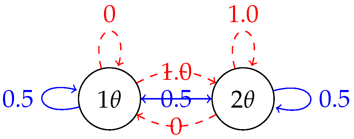
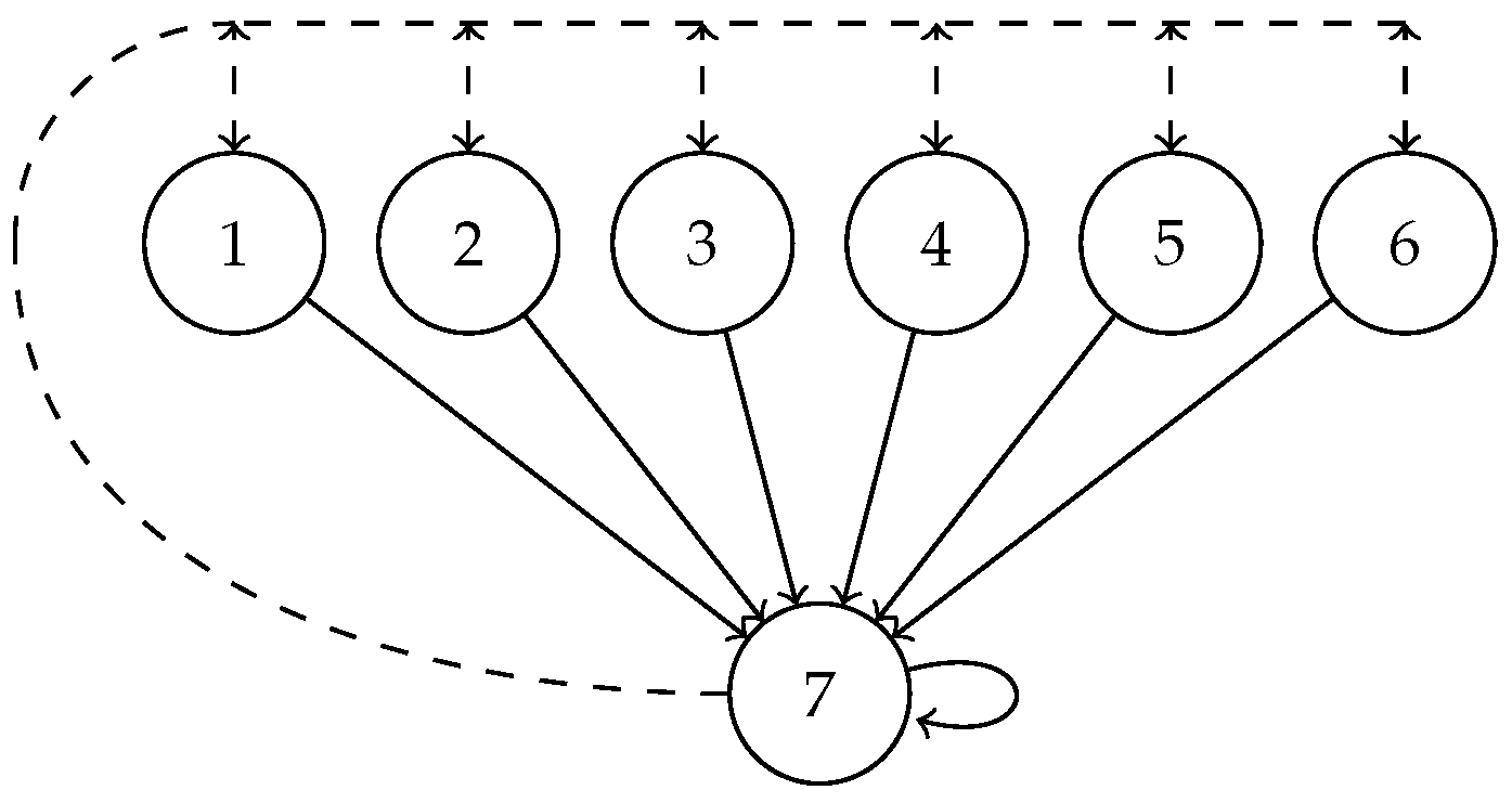
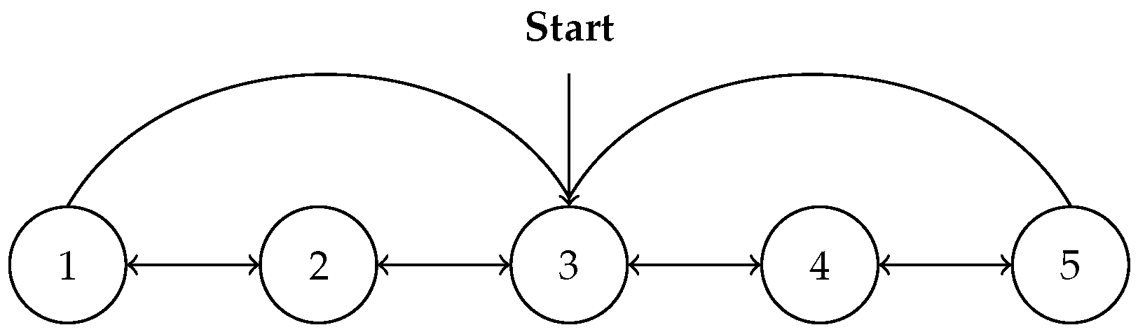
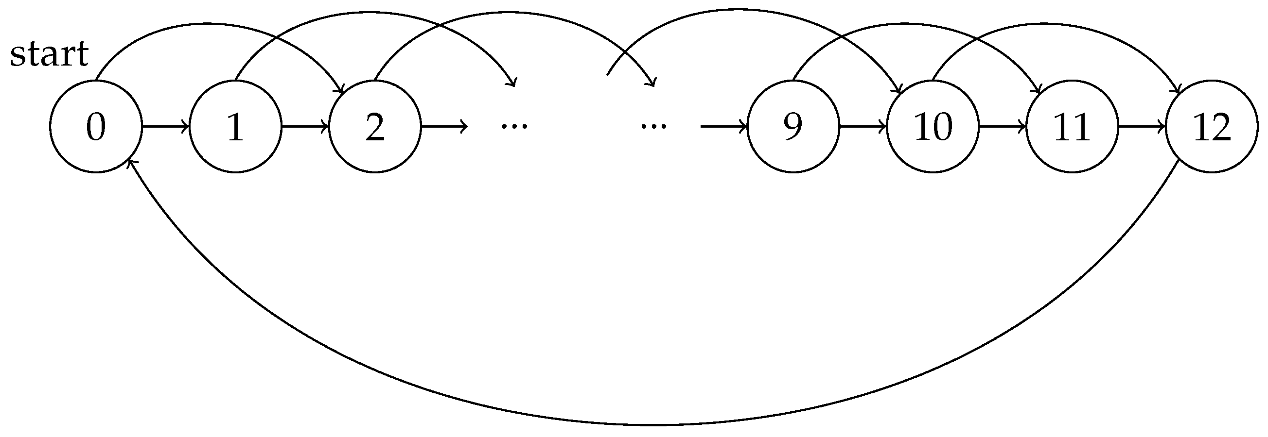
5.1. Example Settings

Two-state counterexample: The $\theta \to 2\theta$ problem has only two states. From each state, there are two actions, left and right, which take the agent to the left or right state. All rewards are zeros. The features $\mathsf{\Phi }={(1,2)}^{\top }$ are assigned to the left and the right state. The schematic of the environment is shown in Figure 1.

The behavior policy takes the equal probability to left or right in both states, i.e., ${\mathrm{P}}_{\mu }=\left[\begin{array}{cc}0.5\hfill & 0.5\hfill \\ 0.5\hfill & 0.5\hfill \end{array}\right].$

The target policy only selects action right in both states, i.e., ${\mathrm{P}}_{\pi }=\left[\begin{array}{cc}0\hfill & 1\hfill \\ 0\hfill & 1\hfill \end{array}\right].$

The state distribution $d_{\mu }={(0.5,0.5)}^{\top }$, $d_x=d_c={(0.5,0.5)}^{\top }$, $\mathbf{C}=2.5$, $f={(0.5,9.5)}^{\top }$, $r_{\pi }=0$, $r_c=0$.

Baird’s counterexample: Baird’s counterexample has seven states, and the schematic of the environment is shown in Figure 2.

The feature matrix is of dimensions $(7\times 8)$ where each state is represented by an 8-dimensional feature, i.e.,

$$\mathsf{\Phi }=\left[\begin{array}{cccccccc}2& 0& 0& 0& 0& 0& 0& 1\\ 0& 2& 0& 0& 0& 0& 0& 1\\ 0& 0& 2& 0& 0& 0& 0& 1\\ 0& 0& 0& 2& 0& 0& 0& 1\\ 0& 0& 0& 0& 2& 0& 0& 1\\ 0& 0& 0& 0& 0& 2& 0& 1\\ 0& 0& 0& 0& 0& 0& 1& 2\end{array}\right].$$

The behavior policy takes equal probabilities to each state, i.e.,

$${\mathrm{P}}_{\mu }=\left[\begin{array}{ccccccc}{\displaystyle \frac{1}{7}}& {\displaystyle \frac{1}{7}}& {\displaystyle \frac{1}{7}}& {\displaystyle \frac{1}{7}}& {\displaystyle \frac{1}{7}}& {\displaystyle \frac{1}{7}}& {\displaystyle \frac{1}{7}}\\ {\displaystyle \frac{1}{7}}& {\displaystyle \frac{1}{7}}& {\displaystyle \frac{1}{7}}& {\displaystyle \frac{1}{7}}& {\displaystyle \frac{1}{7}}& {\displaystyle \frac{1}{7}}& {\displaystyle \frac{1}{7}}\\ {\displaystyle \frac{1}{7}}& {\displaystyle \frac{1}{7}}& {\displaystyle \frac{1}{7}}& {\displaystyle \frac{1}{7}}& {\displaystyle \frac{1}{7}}& {\displaystyle \frac{1}{7}}& {\displaystyle \frac{1}{7}}\\ {\displaystyle \frac{1}{7}}& {\displaystyle \frac{1}{7}}& {\displaystyle \frac{1}{7}}& {\displaystyle \frac{1}{7}}& {\displaystyle \frac{1}{7}}& {\displaystyle \frac{1}{7}}& {\displaystyle \frac{1}{7}}\\ {\displaystyle \frac{1}{7}}& {\displaystyle \frac{1}{7}}& {\displaystyle \frac{1}{7}}& {\displaystyle \frac{1}{7}}& {\displaystyle \frac{1}{7}}& {\displaystyle \frac{1}{7}}& {\displaystyle \frac{1}{7}}\\ {\displaystyle \frac{1}{7}}& {\displaystyle \frac{1}{7}}& {\displaystyle \frac{1}{7}}& {\displaystyle \frac{1}{7}}& {\displaystyle \frac{1}{7}}& {\displaystyle \frac{1}{7}}& {\displaystyle \frac{1}{7}}\\ {\displaystyle \frac{1}{7}}& {\displaystyle \frac{1}{7}}& {\displaystyle \frac{1}{7}}& {\displaystyle \frac{1}{7}}& {\displaystyle \frac{1}{7}}& {\displaystyle \frac{1}{7}}& {\displaystyle \frac{1}{7}}\end{array}\right].$$

The target policy only selects the action to state 7 in both states, i.e.,

$${\mathrm{P}}_{\pi }=\left[\begin{array}{ccccccc}0& 0& 0& 0& 0& 0& 1\\ 0& 0& 0& 0& 0& 0& 1\\ 0& 0& 0& 0& 0& 0& 1\\ 0& 0& 0& 0& 0& 0& 1\\ 0& 0& 0& 0& 0& 0& 1\\ 0& 0& 0& 0& 0& 0& 1\\ 0& 0& 0& 0& 0& 0& 1\end{array}\right].$$

The state distribution

$$d_{\mu }={({\displaystyle \frac{1}{7}},{\displaystyle \frac{1}{7}},{\displaystyle \frac{1}{7}},{\displaystyle \frac{1}{7}},{\displaystyle \frac{1}{7}},{\displaystyle \frac{1}{7}},{\displaystyle \frac{1}{7}})}^{\top },$$

$$d_x=d_c={({\displaystyle \frac{1}{7}},{\displaystyle \frac{1}{7}},{\displaystyle \frac{1}{7}},{\displaystyle \frac{1}{7}},{\displaystyle \frac{1}{7}},{\displaystyle \frac{1}{7}},{\displaystyle \frac{1}{7}})}^{\top },$$

$$\mathbf{C}=\left[\begin{array}{ccccccc}0.571& 0& 0& 0& 0& 0& 0.286\\ 0& 0.571& 0& 0& 0& 0& 0.286\\ 0& 0& 0.571& 0& 0& 0& 0.286\\ 0& 0& 0& 0.571& 0& 0& 0.286\\ 0& 0& 0& 0& 0.571& 0& 0.286\\ 0& 0& 0& 0& 0& 0.571& 0.286\\ 0.286& 0.286& 0.286& 0.286& 0.286& 0.286& 1.429\end{array}\right].$$

$f={({\displaystyle \frac{1}{7}},{\displaystyle \frac{1}{7}},{\displaystyle \frac{1}{7}},{\displaystyle \frac{1}{7}},{\displaystyle \frac{1}{7}},{\displaystyle \frac{1}{7}},{\displaystyle \frac{64}{7}})}^{\top },$$r_{\pi }={(0,0,0,0,0,0,0)}^{\top },$$r_c={(0,0,0,0,0,0,0)}^{\top }.$

Random Walk: Random Walk is centered around a typical Markov Chain. This chain comprises five consecutive states, with two terminal states positioned at each extremity serving as absorptive endpoints.

The schematic of the environment is shown in Figure 3.

Specifically, its state–state transfer probability of behavior policy is

$${\mathrm{P}}_{\mu }=\left[\begin{array}{ccccc}0& 0.6& 0.4& 0& 0\\ 0.4& 0& 0.6& 0& 0\\ 0& 0.4& 0& 0.6& 0\\ 0& 0& 0.4& 0& 0.6\\ 0& 0& 0.6& 0.4& 0\end{array}\right].$$

The state–state transfer probability of the target policy is

$${\mathrm{P}}_{\pi }=\left[\begin{array}{ccccc}0& 0.5& 0.5& 0& 0\\ 0.5& 0& 0.5& 0& 0\\ 0& 0.5& 0& 0.5& 0\\ 0& 0& 0.5& 0& 0.5\\ 0& 0& 0.5& 0.5& 0\end{array}\right].$$

The state distribution $d_{\mu }={({\displaystyle \frac{1}{9}},{\displaystyle \frac{2}{9}},{\displaystyle \frac{3}{9}},{\displaystyle \frac{2}{9}},{\displaystyle \frac{1}{9}})}^{\top }$, $d_c=(0.9$, $0.9$, $0.9$, $0.9$, ${0.9)}^{\top }$, $d_c=({\displaystyle \frac{5}{6}}$, ${\displaystyle \frac{5}{6}}$, ${\displaystyle \frac{5}{6}}$, ${\displaystyle \frac{5}{6}}$, ${\displaystyle \frac{5}{6}}{)}^{\top }$, $f=(0.773$, $1.84$, $3.333$, $2.56$, ${1.493)}^{\top }$, $r_{\pi }=(-0.4$, 0, 0, 0, ${0.6)}^{\top }$, $r_c=(-0.4$, 0, 0, 0, ${0.5)}^{\top }$.

The Random Walk environment has three feature representations, which are called tabular features, inverted features, and dependent features. The feature matrix of Random Walk with tabular features is

$$\mathsf{\Phi }=\left[\begin{array}{ccccc}1& 0& 0& 0& 0\\ 0& 1& 0& 0& 0\\ 0& 0& 1& 0& 0\\ 0& 0& 0& 1& 0\\ 0& 0& 0& 0& 1\end{array}\right].$$

$$\mathbf{C}=\left[\begin{array}{ccccc}0.111& 0& 0& 0& 0\\ 0& 0.222& 0& 0& 0\\ 0& 0& 0.333& 0& 0\\ 0& 0& 0& 0.222& 0\\ 0& 0& 0& 0& 0.111\end{array}\right].$$

The feature matrix of Random Walk with inverted features is

$$\mathsf{\Phi }=\left[\begin{array}{ccccc}0& 0.5& 0.5& 0.5& 0.5\\ 0.5& 0& 0.5& 0.5& 0.5\\ 0.5& 0.5& 0& 0.5& 0.5\\ 0.5& 0.5& 0.5& 0& 0.5\\ 0.5& 0.5& 0.5& 0.5& 0\end{array}\right].$$

$$\mathbf{C}=\left[\begin{array}{ccccc}0.222& 0.167& 0.139& 0.167& 0.194\\ 0.167& 0.194& 0.111& 0.139& 0.167\\ 0.139& 0.111& 0.167& 0.111& 0.139\\ 0.167& 0.139& 0.111& 0.194& 0.167\\ 0.194& 0.167& 0.139& 0.167& 0.222\end{array}\right].$$

The feature matrix of Random Walk with dependent features is

$$\mathsf{\Phi }=\left[\begin{array}{ccc}1& 0& 0\\ {\displaystyle \frac{1}{\sqrt{2}}}& {\displaystyle \frac{1}{\sqrt{2}}}& 0\\ {\displaystyle \frac{1}{\sqrt{3}}}& {\displaystyle \frac{1}{\sqrt{3}}}& {\displaystyle \frac{1}{\sqrt{3}}}\\ 0& {\displaystyle \frac{1}{\sqrt{2}}}& {\displaystyle \frac{1}{\sqrt{2}}}\\ 0& 0& 1\end{array}\right].$$

$$\mathbf{C}=\left[\begin{array}{ccc}0.333& 0.222& 0.111\\ 0.222& 0.333& 0.222\\ 0.111& 0.222& 0.333\end{array}\right].$$

Boyan Chain: The Boyan Chain consists of 13 states, each of which is represented by 4 state features. The feature matrix of the Boyan Chain with dependent features is

$$\mathsf{\Phi }=\left[\begin{array}{cccc}1& 0& 0& 0\\ 0.75& 0.25& 0& 0\\ 0.5& 0.5& 0& 0\\ 0.25& 0.75& 0& 0\\ 0& 1& 0& 0\\ 0& 0.75& 0.25& 0\\ 0& 0.5& 0.5& 0\\ 0& 0.25& 0.75& 0\\ 0& 0& 1& 0\\ 0& 0& 0.75& 0.25\\ 0& 0& 0.5& 0.5\\ 0& 0& 0.25& 0.75\\ 0& 0& 0& 1\end{array}\right].$$

The state distribution $d_{\mu }=(0.108$, $0.054$, $0.081$, $0.068$, $0.075$, $0.071$, $0.073$, $0.072$, $0.072$, $0.072$, $0.072$, $0.072$, ${0.108)}^{\top },$ $d_x$$=d_c$$=(1$, 1, 1, 1, 1, 1, 1, 1, 1, 1, 1, 1, ${1)}^{\top },$

$$\mathbf{C}=\left[\begin{array}{cccc}0.163& 0.043& 0& 0\\ 0.043& 0.199& 0.045& 0\\ 0& 0.045& 0.199& 0.045\\ 0& 0& 0.045& 0.172\end{array}\right].$$

$f={(1.084,0.542,0.813,0.678,0.745,0.712,0.729,0.72,0.724,0.722,0.723,0.723,1.084)}^{\top }$, $r_{\pi }=r_c={(-3,-3,-3,-3,-3,-3,-3,-3,-3,-3,-3,-2,0)}^{\top }.$

Then, the state–state transfer probability of behavior policy is the same as the state–state transfer probability of target policy, i.e., ${\mathrm{P}}_{\mu }={\mathrm{P}}_{\pi }$, where the element of matrix ${\mathrm{P}}_{\mu }$ is as follows, for $i,j\in [0,12]$:

$$P_{\mu }[i,j]=\left\{\begin{array}{cc}0.5\hfill & \mathrm{if}i\le 10\mathrm{and}j=i+1\hfill \\ 0.5\hfill & \mathrm{if}i\le 10\mathrm{and}j=i+2\hfill \\ 1\hfill & \mathrm{if}i=11\mathrm{and}j=12\hfill \\ 1\hfill & \mathrm{if}i=12\mathrm{and}j=0\hfill \\ 0\hfill & \mathrm{otherwise}.\hfill \end{array}\right.$$

The schematic of the environment is shown in Figure 4.

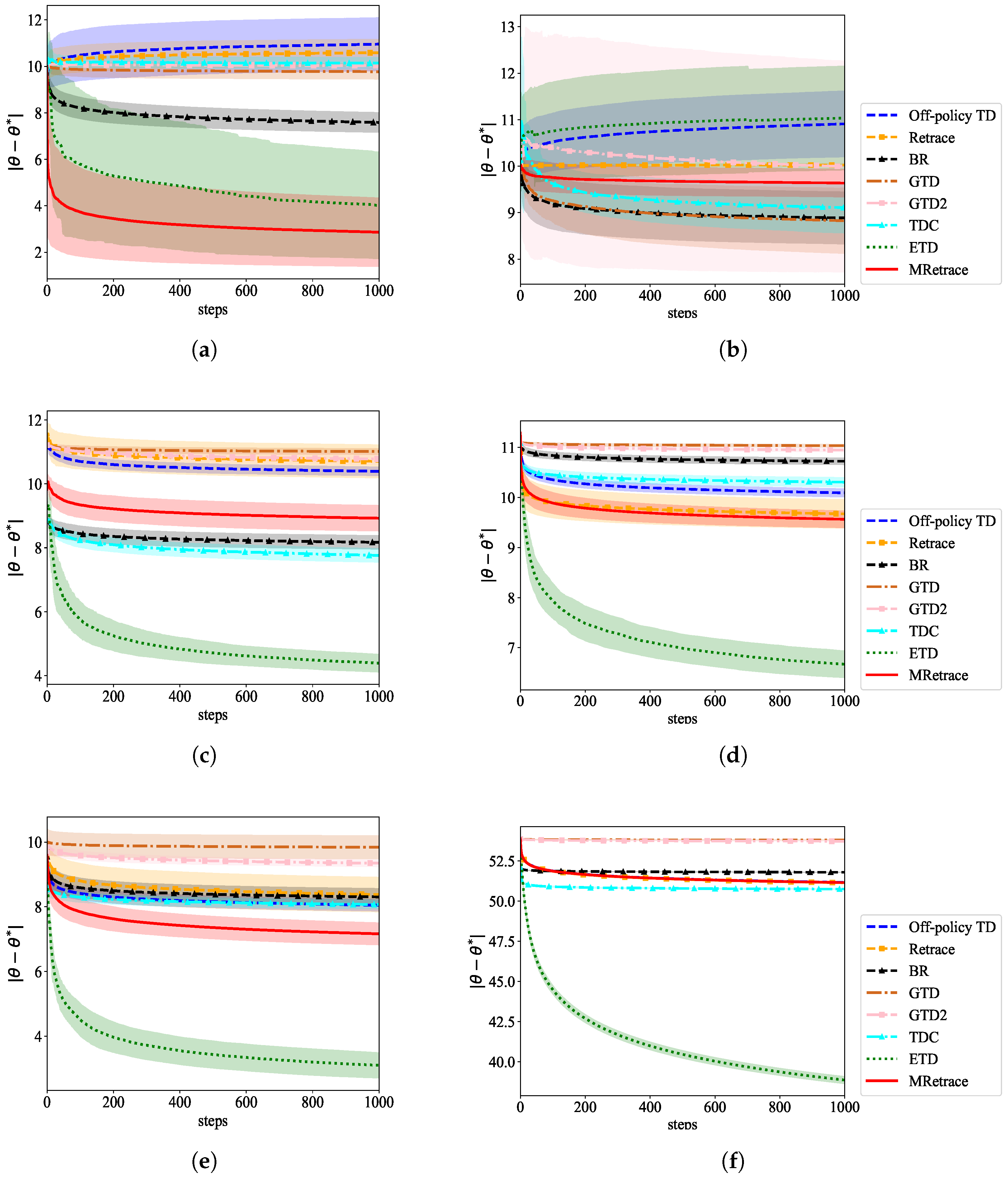
5.2. Results and Analysis

Based on Table 1, first, we need to set $\mathsf{\Phi }$, $P_{\mu }$, $P_{\pi }$, $D_c$, $r_c$, $r_{\pi }$, C, $D_f$, and $D_x$ for each setting. Then, based on the property $d_{\mu }={\mathbf{P}}_{\mu }^{\top }{d}_{\mu }$, we compute the eigenvector of the matrix ${\mathbf{P}}_{\mu }^{\top }$ with eigenvalue 1.0, and we unitize it to obtain $d_{\mu }$ and $D_{\mu }$. (It is important to note that when there are absorbing states in a Markov Chain, the probability distribution is 1.0 only at the absorbing states and 0 at all other states. Therefore, we adopt a restart approach, jumping directly back to the initial states, thus forming a probability transition matrix ${\mathbf{P}}_{\mu }$ without absorbing states.) After all, we compute the key matrix for each algorithm and its minimum eigenvalue. Note that the step-size ratio $\eta$ of the auxiliary parameter to the learning parameter is usually set to $\eta \ge 1.0$.

The minimum eigenvalues in several examples for each algorithm are summarized in

Table 2. Minimum eigenvalues ${\displaystyle \frac{1}{2}}{\lambda }_{min}(\mathbf{A}+{\mathbf{A}}^{\top })$ of various algorithms on several examples.

Algorithm	Two-State	Baird’s	Random Walk			Boyan Chain
			Tabular	Inverted	Dependent
Off-policy TD	$-0.2$	$-0.791$	$0.018$	$0.017$	$0.07$	$0.024$
Retrace	$-0.1$	$-0.113$	$0.017$	$0.015$	$0.063$	$0.024$
BR	$0.34$	9.673 × 10−17	$0.002$	$0.007$	$0.033$	$0.002$
GTD	0	0	0	0	0	0
GTD2	0	−1.077 × 10−17	0	0	0	0
TDC	$0.016$	$-0.002$	$0.002$	$0.007$	$0.011$	$0.002$
ETD	$\mathbf{3}.\mathbf{4}$	−2.82 × 10−16	$\mathbf{0}.\mathbf{195}$	$\mathbf{0}.\mathbf{165}$	$\mathbf{0}.\mathbf{76}$	$\mathbf{0}.\mathbf{245}$
MRetrace	$1.15$	−2.141 × 10−17	$0.046$	$0.02$	$0.094$	$0.024$

. We can find the following: (1) In Baird’s counterexample and a two-state counterexample, the minimum eigenvalues of key matrices in off-policy TD and Retrace are both less than 0, indicating that they will diverge in these two counterexamples, which is consistent with the existing research [2]. Additionally, compared with off-policy TD, Retrace does have some mitigation towards divergence but cannot avoid it.

(2) In Baird’s counterexample, the minimum eigenvalues of GTD2, TDC, ETD, and MRetrace are all less than zero, indicating that their key matrices are not positive definite. This seems inconsistent with our understanding. The main reason is that in Baird’s counterexample, the feature matrix is $7\times 8$, and is not column full rank, which is inconsistent with the assumption in their theorems. Note that the absolute value of the minimum eigenvalue is very small.

(3) Except for Baird’s counterexample, the minimum eigenvalues of GTD and GTD2 are all zeros. The reason is that matrices ${\displaystyle \frac{1}{2}}{\lambda }_{min}(\mathbf{A}+{\mathbf{A}}^{\top })$ of GTD and GTD2 are positive semi-definite. In the context of this paper, we are unable to distinguish which one is faster between GTD and GTD2 in numerical analysis.

(4) The minimum eigenvalue of TDC is higher than GTD and GTD2, which is consistent with the literature.

(5) Except for Baird’s counterexample, the minimum eigenvalue of ETD is the largest.

(6) Except for Baird’s counterexample, MRetrace has the second-largest minimum eigenvalues.

(7) All the minimum eigenvalues of BR are greater than 0, making it the only one to remain positive definite in all examples. However, except for Baird’s counterexample, its minimum eigenvalue is not large.

(8) The Boyan Chain is an on-policy setting; off-policy TD is implemented in on-policy; and off-policy TD, Retrace, and MRetrace have the same minimum eigenvalue of 0.024. BR and TDC have the same minimum eigenvalue of 0.002, indicating that BR and TDC are not suitable for on-policy learning.

(9) It is surprising that in an on-policy setting, the minimum eigenvalue of ETD is larger than that of on-policy TD. This implies that in terms of the expected convergence rate, ETD is the most recommended option for on-policy learning.

To the best of our knowledge, this is the first time that various temporal difference learning algorithms have been compared for their convergence rates in a very intuitive numerical analysis manner.

In summary, in the expected sense, ETD has the fastest convergence rate, followed by MRetrace.

6. Experimental Studies

In Section 3, we proposed Corollary 2, and in Section 4, we compared the sizes of the minimum eigenvalues of different algorithms for various environment settings. This means that we carried out theoretical analysis combined with numerical analysis, but whether the analytical results reflect the actual situation needs to be experimentally verified. Therefore, we adopted the same environment settings as in Section 4.

Each algorithm runs independently 20 times, with 1000 steps per run, and calculates the mean and standard deviation.

To compare convergence rates, we need to observe the trend of $|{\theta }_t-{\theta }^{\ast }|$ over time step t. Note that according to Table 1, different algorithms have different optimal solutions ${\theta }^{\ast }={\mathbf{A}}^{-1}\mathbf{b}$, so we need to calculate their optimal solutions separately for each algorithm and then measure the errors.

The learning rate is set to satisfy Assumption 3, ${\alpha }_t={\alpha }_0\times {\displaystyle \frac{1}{t+1}}$, where ${\alpha }_0$ is an initial learning rate. We set $\eta =4$ for GTD and GTD2 in all environments. In two-state counterexamples, ${\alpha }_0=0.1$, and $\gamma =0.9$. In Baird’s counterexamples, ${\alpha }_0=0.05$, and $\gamma =0.99$. In Random Walk, ${\alpha }_0=0.25$, and $\gamma =0.9$. In a Boyan Chain, ${\alpha }_0=0.25$, and $\gamma =0.9$.

The learning curves of different algorithms in different environments are shown in Figure 5, where each curve displays the mean and standard deviation of the errors. We can find the following: (1) In Random Walk with dependent features, the convergence rate analysis is consistent with the learning curves of each algorithm. They have the same order: ETD > MRetrace > off-policy TD > Retrace > TDC ≥ BR > GTD2 ≥ GTD.

(2) Off-policy TD and Retrace diverge in both counterexamples, but Retrace diverges more slowly compared with off-policy TD. This is consistent with the numerical analysis in Section 4.

(3) In Baird’s counterexample, GTD descends faster than GTD2 and TDC. This may be related to the numerical analysis showing that the minimum eigenvalues of GTD2 and TDC are less than 0. Therefore, this is consistent with the analysis.

(4) In Baird’s counterexample, ETD diverges. On the one hand, this is related to high variances of ETD reported in the literature [6,19]; on the other hand, it is also related to the numerical analysis, showing that the minimum eigenvalue is less than 0.

(5) In a two-state counterexample, compared to BR, ETD, and MRetrace, the algorithms GTD, GTD2, and TDC converge very slowly. Additionally, BR converges slower than MRetrace and ETD. These observations are consistent with our numerical analysis. However, ETD is slower than MRetrace, which is attributed to the high variance of ETD.

(6) In Random Walk and the Boyan Chain, TDC converges much faster than GTD and GTD2, which is consistent with our numerical analysis. This observation also aligns with existing research.

(7) In Random Walk and the Boyan Chain, the convergence rate of ETD is remarkably fast, which aligns with our numerical analysis. ETD is reported to be suitable for off-policy learning, but its exceptional performance in on-policy learning is somewhat incredible.

(8) In the Boyan Chain, off-policy TD is implemented as on-policy TD. The learning curves of TD, Retrace, and MRetrace overlap. This is consistent with our numerical analysis.

In conclusion, the convergence rates of the algorithms in the experiments align with the numerical analysis. Moreover, any inconsistencies have interpretable underlying reasons.

7. Conclusions and Future Work

Based on the proposed convergence rate for constructing general off-policy temporal difference learning algorithms, this paper proved that the primary determinant influencing convergence rate is the minimum eigenvalue of the key matrix. Focusing on this factor will be more conducive to the development of faster converging off-policy learning algorithms.

The limitations of this paper include the following aspects:

(1)

This paper assumes that the learning rates of all algorithms are the same; however, in reality, different algorithms have different ranges of applicable learning rates.

(2)

This paper does not consider the scenario of a fixed learning rate.

(3)

This paper focuses on learning prediction and does not address learning control.

Future works need to address the above limitations and explore how to design faster algorithms based on the conclusions of this paper.

In the end, we discovered a contradiction. Sutton et al. [4] proved that ${\mathbf{A}}_{\mathrm{GTD}}=\left(\begin{array}{cc}\sqrt{\eta }\mathbf{I}& {\mathbf{A}}_{\mathrm{off}}\\ -{\mathbf{A}}_{\mathrm{off}}^{\top }& 0\end{array}\right)$ is positive definite. Note that in the paper, $\mathbf{G}=\left(\begin{array}{cc}-\sqrt{\eta }\mathbf{I}& -{\mathbf{A}}_{\mathrm{off}}\\ {\mathbf{A}}_{\mathrm{off}}^{\top }& 0\end{array}\right)$ is proved to be negative definite [4]. According to Theorem A.3 of [20], the positive definiteness of square matrix $\mathbf{A}$ is equivalent to the positive definiteness of $(\mathbf{A}+{\mathbf{A}}^{\top })$; thus, $({\mathbf{A}}_{\mathrm{GTD}}+{\mathbf{A}}_{\mathrm{GTD}}^{\top })$ is positive definite. However, our calculations in this paper showed that $({\mathbf{A}}_{\mathrm{GTD}}+{\mathbf{A}}_{\mathrm{GTD}}^{\top })=\left(\begin{array}{cc}2\sqrt{\eta }\mathbf{I}& 0\\ 0& 0\end{array}\right)$ is positive semi-definite, not positive definite. Therefore, the conclusion that ${\mathbf{A}}_{\mathrm{GTD}}$ is positive definite is questionable.

References

1. Sutton, R.S.; Barto, A.G. Reinforcement Learning: An Introduction, 2nd ed.; The MIT Press: Cambridge, MA, USA, 2018. [Google Scholar]
2. Sutton, R.S.; Mahmood, A.R.; White, M. An emphatic approach to the problem of off-policy temporal-difference learning. J. Mach. Learn. Res. 2016, 17, 2603–2631. [Google Scholar]
3. Baird, L. Residual algorithms: Reinforcement learning with function approximation. In Proceedings of the 12th International Conference on Machine Learning, Tahoe City, CA, USA, 9–12 July 1995; pp. 30–37. [Google Scholar]
4. Sutton, R.S.; Maei, H.R.; Szepesvári, C. A Convergent O(n) Temporal-difference Algorithm for Off-policy Learning with Linear Function Approximation. Adv. Neural Inf. Process. Syst. 2008, 21, 1609–1616. [Google Scholar]
5. Sutton, R.; Maei, H.; Precup, D.; Bhatnagar, S.; Silver, D.; Szepesvári, C.; Wiewiora, E. Fast gradient-descent methods for temporal-difference learning with linear function approximation. In Proceedings of the 26th International Conference on Machine Learning, Montreal, QC, Canada, 14–18 June 2009; pp. 993–1000. [Google Scholar]
6. Chen, X.; Ma, X.; Li, Y.; Yang, G.; Yang, S.; Gao, Y. Modified retrace for off-policy temporal difference learning. In Proceedings of the Thirty-Ninth Conference on Uncertainty in Artificial Intelligence, Pittsburgh, PA, USA, 31 July–4 August 2023; pp. 303–312. [Google Scholar]
7. Dalal, G.; Szörényi, B.; Thoppe, G.; Mannor, S. Finite sample analyses for TD (0) with function approximation. In Proceedings of the AAAI Conference on Artificial Intelligence, New Orleans, LO, USA, 2–7 February 2018; Volume 32. [Google Scholar]
8. Dalal, G.; Thoppe, G.; Szörényi, B.; Mannor, S. Finite sample analysis of two-timescale stochastic approximation with applications to reinforcement learning. In Proceedings of the Conference On Learning Theory, PMLR, Stockholm, Sweden, on 5–9 July 2018; pp. 1199–1233. [Google Scholar]
9. Gupta, H.; Srikant, R.; Ying, L. Finite-time performance bounds and adaptive learning rate selection for two time-scale reinforcement learning. In Proceedings of the 33rd International Conference on Neural Information Processing Systems, Vancouver, BC, Canada, 8–14 December 2019; pp. 4704–4713. [Google Scholar]
10. Xu, T.; Zou, S.; Liang, Y. Two time-scale off-policy TD learning: Non-asymptotic analysis over Markovian samples. In Proceedings of the 33rd International Conference on Neural Information Processing Systems, Vancouver, BC, Canada, 8–14 December 2019; pp. 10634–10644. [Google Scholar]
11. Dalal, G.; Szorenyi, B.; Thoppe, G. A tale of two-timescale reinforcement learning with the tightest finite-time bound. In Proceedings of the AAAI Conference on Artificial Intelligence, New York, NY, USA, 7–8 February 2020; Volume 34, pp. 3701–3708. [Google Scholar]
12. Durmus, A.; Moulines, E.; Naumov, A.; Samsonov, S.; Scaman, K.; Wai, H.T. Tight high probability bounds for linear stochastic approximation with fixed stepsize. Adv. Neural Inf. Process. Syst. 2021, 34, 30063–30074. [Google Scholar]
13. Xu, T.; Liang, Y. Sample complexity bounds for two timescale value-based reinforcement learning algorithms. In Proceedings of the International Conference on Artificial Intelligence and Statistics, PMLR, Virtual, 13–15 April 2021; pp. 811–819. [Google Scholar]
14. Zhang, S.; Des Combes, R.T.; Laroche, R. On the convergence of SARSA with linear function approximation. In Proceedings of the International Conference on Machine Learning, PMLR, Honolulu, HI, USA, 23–29 July 2023; pp. 41613–41646. [Google Scholar]
15. Wang, S.; Si, N.; Blanchet, J.; Zhou, Z. A finite sample complexity bound for distributionally robust q-learning. In Proceedings of the International Conference on Artificial Intelligence and Statistics, PMLR, Honolulu, HI, USA, 23–29 July 2023; pp. 3370–3398. [Google Scholar]
16. Munos, R.; Stepleton, T.; Harutyunyan, A.; Bellemare, M. Safe and efficient off-policy reinforcement learning. Adv. Neural Inf. Process. Syst. 2016, 29, 1054–1062. [Google Scholar]
17. Boyan, J.A. Technical update: Least-squares temporal difference learning. Mach. Learn. 2002, 49, 233–246. [Google Scholar] [CrossRef]
18. Ghiassian, S.; Patterson, A.; Garg, S.; Gupta, D.; White, A.; White, M. Gradient temporal-difference learning with regularized corrections. In Proceedings of the International Conference on Machine Learning, PMLR, Virtual, 13–18 July 2020; pp. 3524–3534. [Google Scholar]
19. Zhang, S.; Whiteson, S. Truncated emphatic temporal difference methods for prediction and control. J. Mach. Learn. Res. 2022, 23, 6859–6917. [Google Scholar]
20. Sutton, R.S. Learning to predict by the methods of temporal differences. Mach. Learn. 1988, 3, 9–44. [Google Scholar] [CrossRef]
Figure 1. Two-state counterexample, where the blue solid arrows represent the behavior policy μ , and the red dashed arrows represent the target policy π .
Mathematics 12 02930 g001
Figure 2. Baird’s counterexample, where the probability of the solid action and the dashed action in behavior policy μ and target policy π are μ ( d a s h e d · ) = 6 7 , μ ( s o l i d · ) = 1 7 and π ( s o l i d · ) = 1 .
Mathematics 12 02930 g002
Figure 3. Random Walk. All walks begin in state 3. Under the behavior policy, take either a left or right action with a probability of 0.5 in each state. Under the target policy, take either a left or right action with a probability of 0.4 or 0.6 in each state.
Mathematics 12 02930 g003
Figure 4. Boyan Chain. In state 0–10, each solid action is taken with probability 0.5. In states 11 and 12, the probability of a solid action is 1.
Mathematics 12 02930 g004
Figure 5. Comparisons of learning curves in different environments. (a) Two-state counterexamples; (b) Baird’s counterexamples; (c) Random Walk with tabular features; (d) Random Walk with inverted features; (e) Random Walk with dependent features; (f) Boyan Chain.
Mathematics 12 02930 g005