Abstract
Network slicing is an advanced technology that significantly enhances network flexibility and efficiency. Recently, reinforcement learning (RL) has been applied to solve resource management challenges in 6G networks. However, RL-based network slicing solutions have not been widely adopted. One of the primary reasons for this is the slow convergence of agents when the Service Level Agreement (SLA) weight parameters in Radio Access Network (RAN) slices change. Therefore, a solution is needed that can achieve rapid convergence while maintaining high accuracy. To address this, we propose a Teacher and Assistant Distillation method based on cosine similarity (TADocs). This method utilizes cosine similarity to precisely match the most suitable teacher and assistant models, enabling rapid policy transfer through policy distillation to adapt to the changing SLA weight parameters. The cosine similarity matching mechanism ensures that the student model learns from the appropriate teacher and assistant models, thereby maintaining high performance. Thanks to this efficient matching mechanism, the number of models that need to be maintained is greatly reduced, resulting in lower computational resource consumption. TADocs improves convergence speed by 81% while achieving an average accuracy of 98%.
MSC:
68T07
1. Introduction
The 6G network addresses diverse service demands by adopting network slicing technology [1], which creates multiple virtual slices on a unified physical network infrastructure. Each slice is optimized for specific service requirements to ensure the Quality of Experience (QoE) for users. Although this technology significantly enhances network flexibility and efficiency, it also faces several challenges. On the one hand, as service demands become increasingly specific, the imbalance in network resource allocation requires timely responses and adjustments, necessitating the optimization of Service Level Agreement (SLA) weights for network slices. This optimization inevitably increases the complexity of network management. On the other hand, to cope with the diversity of service demands, more refined management techniques, such as sub-slicing, may need to be introduced to achieve more detailed resource allocation and service quality control. However, while these refined management methods improve management efficiency, they may also lead to severe resource wastage.
Deep reinforcement learning (DRL), with its exceptional adaptability and decision optimization capabilities, has attracted widespread attention from researchers in the field of network resource allocation [2,3]. Particularly, with the advancement of the Open Radio Access Network (O-RAN) architecture, mobile network operators (MNOs) can more effectively meet the specific demands of different network slices, thereby significantly enhancing their control over network resources. However, when faced with the challenge of abrupt changes in the SLA weights of slices in the Radio Access Network (RAN), traditional DRL methods often lack the necessary flexibility. Although techniques such as parameter initialization have been proposed to accelerate the DRL convergence process, these methods typically still require substantial computational resources and time, making it difficult to meet the high demands of real-time network responses.
Given these challenges, it is crucial to develop more efficient methods to accelerate reinforcement learning convergence and improve accuracy. Knowledge Distillation (KD) is an effective technique for transferring knowledge from a complex teacher model, trained on large datasets, to a simpler student model. This process retains high accuracy while significantly reducing the student model’s training time [4]. However, KD has limitations; if the teacher model suffers from overfitting or inductive biases [5], these issues can also be passed to the student, affecting performance. While multi-teacher distillation methods aim to optimize knowledge transfer by assigning weights to different teachers, merely learning from multiple teachers does not always lead to improved performance.
Thus, there is an urgent need for a method that can quickly adapt to changes in RAN slice SLA weights while ensuring model accuracy with low time and computational costs, effectively addressing the diverse demands in dynamic network environments.
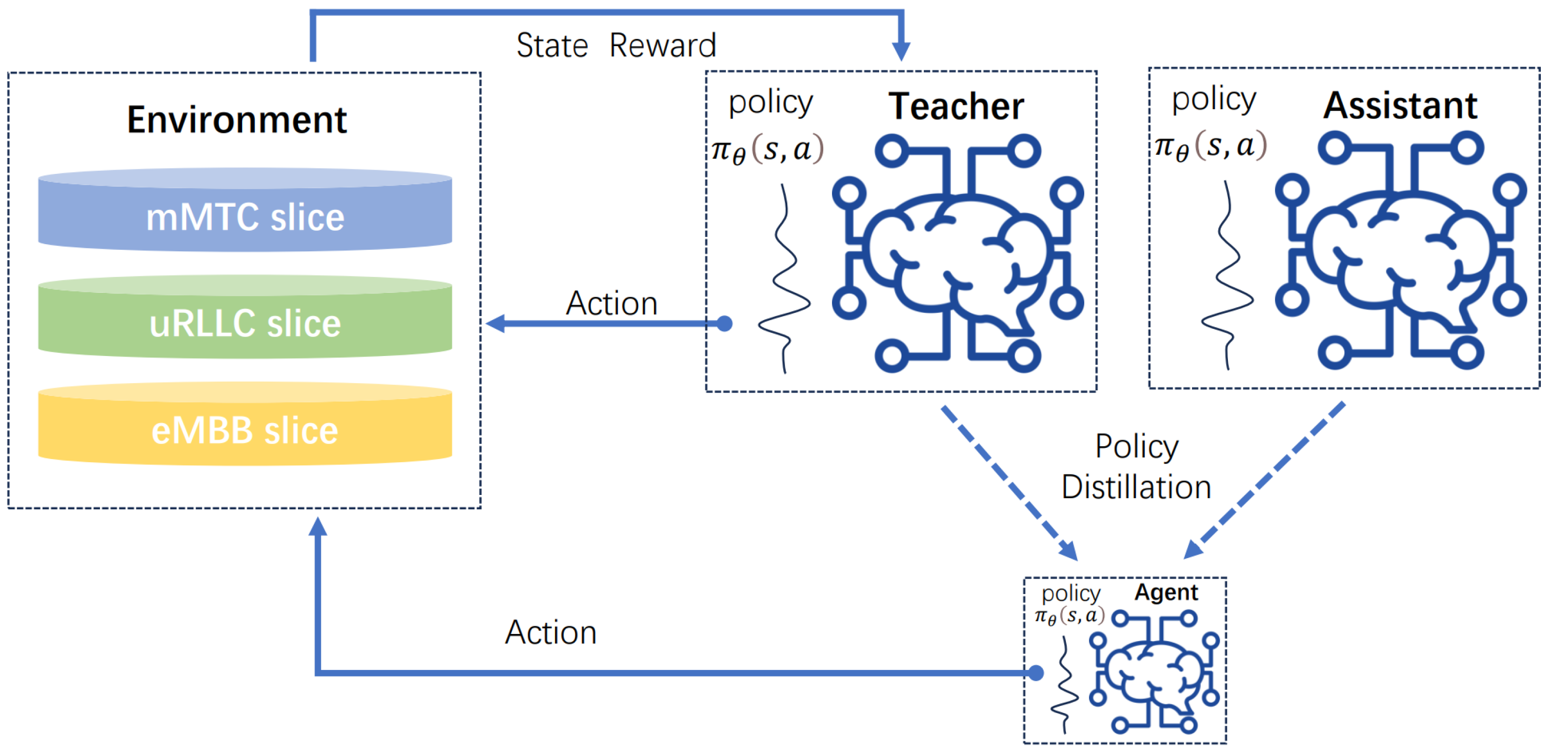
This study proposes a novel Teacher and Assistant Distillation (TADocs) framework based on cosine similarity to address the challenges in RANs, the diagram is shown in Figure 1. We used DRL techniques to train teacher models for different RAN slice SLA weights. When slice weights changed, the most suitable teacher and assistant models were selected using cosine similarity, and their knowledge was transferred to the new model via policy distillation. This approach improves DRL agent convergence and adaptability while reducing resource consumption. It also mitigates inductive bias from relying on a single teacher model.
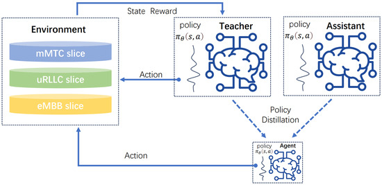
Figure 1.
Diagram of TADocs architecture.
The contributions of this study are as follows:
- 1.
- This study proposes a rapid knowledge transfer method that ensures fast convergence and maintains high performance under dynamic SLA weight adjustments by Mobile Network Operators.
- 2.
- By applying cosine similarity to match the most suitable models as teachers and assistants, the demand for the number of pre-trained models is considerably reduced, thereby substantially decreasing the consumption of computational resources and time.
- 3.
- The introduction of the teacher and assistant policy distillation mechanism effectively avoids the inductive bias that may arise from learning from a single teacher, endowing the student model with high adaptability and accuracy.
The rest of the paper is organized as follows. In Section 2, we review the related work. The system model and formulation are described in Section 3. In Section 4, we propose and introduce TADocs in detail. Section 5 presents an analysis of the experimental results. Finally, in Section 6, we conclude our work and discuss potential future directions.
2. Related Work
Traditional network slicing management methods mainly rely on static configurations and pre-planned policies to ensure customized services, isolation, and multi-tenancy support on shared physical network infrastructure through logical separation of network resources [6], the illustration is shown in Figure 2. These methods typically utilize fixed resource allocation mechanisms, dividing network resources into multiple slices based on historical data and experience, with each slice corresponding to specific services or applications. This approach works effectively under stable network loads and relatively uniform service demands, but it falls short in the face of rapidly changing service demands in the 6G and cloud computing era, lacking the flexibility for real-time adjustments. Additionally, this static allocation method may lead to resource under-utilization or resource shortages during peak times [7]. Furthermore, traditional methods struggle to address the complex demands in multi-tenant environments, failing to effectively isolate interference between different tenants, leading to a decline in Quality of Service (QoS). This is reflected in various aspects such as response time, cost, throughput, performance, and resource utilization [8]. To address these issues, researchers have proposed enhancements to traditional methods, such as by introducing policy-based management, which dynamically adjusts resource allocation through predefined rules and conditions [9]. However, even with the adoption of these methods, traditional network slicing management approaches still struggle to fully meet the highly dynamic and diverse requirements of the 6G dynamic networking environment [10]. This has driven the exploration of more advanced management technologies, such as AI-based dynamic resource management solutions, to achieve more efficient and intelligent RAN slicing management.
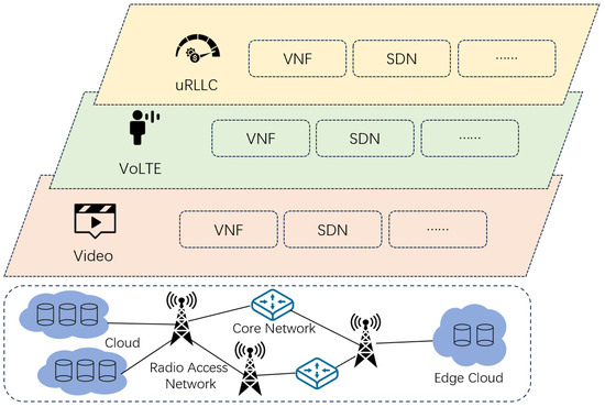
Figure 2.
Illustration of RAN slices.
Reinforcement Learning (RL), as a significant branch of artificial intelligence, has demonstrated unique value across various domains. In the task of network resource allocation, DRL has shown remarkable effects in optimizing network performance due to its excellent adaptability and decision efficiency. This advanced technology can dynamically adjust resource allocation strategies to adapt to the constantly changing network environment and user demands, ensuring the efficient utilization of network resources [11]. The emergence of the O-RAN architecture allows mobile network operators (MNOs) to better meet the demands of different network slices, thereby enhancing their control over the network [12]. Xie et al. used an improved Dueling-DQN algorithm to enhance slice performance in dynamic multi-tenant network environments [13]. Huang et al. achieved real-time and adaptive resource allocation through collaborative RL and edge intelligence (EI) technologies [14]. Wang et al. proposed an innovative 5G network slicing resource scheduling strategy that does not rely on predefined models but uses deep convolutional neural networks (CNNs) to capture the complexities of the 5G network environment and optimize resource allocation for each slice accordingly [15]. Zhu have proposed that RL can achieve a better initial performance through knowledge transfer, typically requiring fewer interactions compared to learning from scratch [16].
Knowledge distillation technology, proposed by Geoffrey Hinton in 2015, has been widely applied across diverse fields. It is a natural idea to leverage this technology and utilize valuable experience to accelerate the training process [17]. Through knowledge distillation, smaller neural networks are capable of acquiring generalization capabilities similar to those of larger networks [4,18]. In the field of network resource management, Jang et al. utilized knowledge distillation to transfer deep reinforcement learning knowledge from the cloud to resource-constrained edge computing systems, realizing substantial model compression effects [19]. As distillation technology has further developed, it has evolved from the initial one-to-one distillation to many-to-one distillation. Yuan et al. modeled the process of assigning weights to different teacher models as a reinforcement learning task to compress large language models and improve their accuracy, successfully optimizing model performance [20]. In the field of image recognition, Zhang et al. improved distillation effects through multi-teacher distillation. They adaptively adjusted the weights of each teacher model based on the comparison accuracy between the teacher model outputs and the ground truth for each sample, effectively boosting the performance of the distillation process [21].
Reinforcement learning and knowledge distillation, among other artificial intelligence technologies, provide advanced methods and superior performance for RAN slicing management. Despite the significant potential of DRL in applications, the challenges it faces cannot be ignored. One major limitation of DRL is the long convergence time, which affects its efficiency in scenarios requiring swift responses. Additionally, when the SLA weights change, pre-trained RL agents often struggle to adapt to the new network slicing environment, requiring retraining [22]. These challenges increase the complexity and uncertainty of deploying DRL technology in practical network systems, limiting its widespread application.
Therefore, DRL needs to quickly adapt to new network slicing environments. In the future development of 6G networks, they are expected to feature massive bandwidth, ultra-low latency, and deep integration of AI technology. At the same time, reinforcement learning can be used to train the network to make optimal decisions, enhancing overall performance [23]. The challenge is how to minimize the agent’s convergence time while maintaining high accuracy, ensuring that the agent can swiftly adapt to new SLA weight configurations and maintain high QoS [24]. To address this issue, Nagib et al. proposed an effective solution. This method first pre-trains 16 teacher models, each corresponding to a specific slice weight configuration. When the slice weights change, a predictive strategy is used to select the best-matching teacher model and copy its trained weight parameters to the new model, followed by subsequent training. This approach shortens training time and reduces the consumption of computational resources and time to some extent. However, this method also has limitations. Firstly, maintaining 16 teacher models is required. Secondly, it may not ensure that each new slice weight finds a well-matched teacher model. Finally, the matched teacher model’s parameters need to be copied to the student model before further training [22].
We conducted a systematic review of network slicing optimization techniques in chronological order, and summarized the advantages and disadvantages of each method in Table 1.

Table 1.
Summary of methods, advantages, and disadvantages proposed by different researchers.
3. System Model and Formulation
In this section, we introduce the system model under consideration and formulate it as a mathematical optimization problem.
3.1. Network Slice Resources
RAN slicing virtualizes the physical network into multiple logical networks, each slice operating independently to meet different QoS requirements. Suppose there are N slices in total, and the system needs to dynamically allocate resources R to each slice i to satisfy its QoS demands. The total resources R refer to the overall resources available within each Transmission Time Interval (TTI). These resources can specifically refer to bandwidth, delay, packet loss rate, etc.
Let the resource allocation vector be , where represents the amount of resources allocated to the i-th slice. The system’s resource constraint is given by:
where is the total amount of system resources.
3.2. Service Level Agreement
A Service Level Agreement (SLA) is a set of clearly defined service delivery requirements and standards that ensure a common understanding of service quality, performance, and responsibilities between customers and service providers. SLAs typically include service descriptions, performance standards, responsibilities and obligations, monitoring and reporting methods, and corrective actions for unmet standards. These elements ensure service transparency and measurability, helping to prevent and resolve delivery disputes [25].
In network slicing management, SLAs are used to define the Quality of Service (QoS) requirements for each slice. Suppose there are N slices in the system, the QoS requirements for each slice i can be represented as a set of constraints:
where represents the bandwidth resources allocated to the i-th slice, and is its minimum bandwidth requirement. represents the delay of the i-th slice, and is its maximum acceptable delay. represents the packet loss rate of the i-th slice, and is its maximum acceptable packet loss rate.
The SLA for the entire system can be expressed as:
which means that the QoS requirements of all slices must be simultaneously satisfied.
In the operations of MNOs, SLAs are often adjusted based on the overall QoE of the network. Some researchers consider a RAN slicing scenario in which MNOs can change the priorities of fulfilling the SLAs of the available slices [26]. This can be done by tuning the weights of the corresponding KPIs in the RL reward function for each slice [22].
In our research, taking a specific weight configuration as an example, the weights for voice over LTE (VoLTE), ultra-reliable low-latency communication (uRLLC), and video are 0.3, 0.6, and 0.1, respectively. This weight configuration is represented as slice = [0.3, 0.6, 0.1] and is referred to as the SLA weight. The RL agent trained under this weight configuration can efficiently handle the corresponding service demands according to the SLA. However, when the slice weights change, for example, during the operation of MNOs, the SLAs may be adjusted based on the overall QoE of the network. The new SLA weights may be represented as slice_new = [0.8, 0.1, 0.1]. Hereafter, we will consistently use this method to represent the SLA weights of network slices.
3.3. RL-Based Slicing
RL is a subfield of artificial intelligence that differs from supervised learning. It focuses on training an agent to learn optimal policies through interactions with the environment to maximize cumulative rewards. Centered on decision-making processes, RL is typically modeled as a Markov Decision Process (MDP). The goal of RL can be formalized as learning a policy that maximizes the expected return:
3.3.1. State Space
The definition of the state space is represented by the proportion of demand for different types of services in the system. Our study includes the following three types of these services: VoLTE, uRLLC, and video. Specifically, the state space consists of three elements, each representing the relative demand for a service type at the current time step. These relative demands are calculated by dividing the total demand for each service by the total demand of all services. At each time step t, the state vector is composed of the relative demands of the three service types. These relative demands are calculated by dividing the total demand for each service by the total demand of all services. The specific definition is as follows:
Assume that the demands for the three service types at time step t are , , and , respectively. The total demand is expressed as:
If the total demand is not zero, the relative demand is calculated by the following formulas:
The relative demand for VoLTE:
The relative demand for uRLLC:
The relative demand for video:
The state vector is expressed as:
The state vector is generated at each time step and is returned to the agent for the next decision. This state vector reflects the relative demand of the three types of services in the current system and is an important basis for resource allocation decisions.
3.3.2. Action Space
The action space is defined through different resource allocation strategies. Each action corresponds to a specific resource allocation ratio, distributing available resources to the three following different service type slices: VoLTE, uRLLC, and video.
Assume the total resource amount is R, with the three service slices being VoLTE, uRLLC, and video. The action space is defined to include all resource allocation actions. Each action corresponds to a resource allocation vector , whose elements represent the proportion of resources allocated to each service type.
The specific definition is as follows:
The total resource amount R is expressed as:
This means that within each TTI, the maximum amount of resources the network can provide is defined as max_size_per_tti. By clearly defining the total resource amount R, a unified benchmark is ensured for resource allocation, facilitating the management and optimization of network resource usage.
The resource allocation vector is , where represent the resource proportions allocated to VoLTE, uRLLC, and Video, respectively.
Each action a in the action space is defined as a resource allocation strategy. Within this framework, the reinforcement learning algorithm dynamically adjusts resource allocation by selecting actions , optimizing the resource utilization and user QoE.
3.3.3. Reward Function
The reward function is used in reinforcement learning to measure the immediate return an agent receives after taking a specific action in a particular state. In the context of RAN slicing, the reward function is used to assess the effectiveness of different resource allocation strategies, thereby guiding the optimization process. Our reward function considers the waiting times for each type of service, and they are weighted and summed accordingly.
At time step t, for the three service types, VoLTE, uRLLC, and video, the weights are normalized. The reward function can be expressed as:
where:
Specifically, corresponds to the importance of the delay time for each slice, and L represents the reciprocal of the available slice delay.
The optimization objective is to find a resource allocation strategy that maximizes the reward function, thereby minimizing the total service processing time, that is:
4. Details of TADocs
In the RAN slicing scenario, we propose the TADocs (Teacher and Assistant Distillation based on cosine similarity) reinforcement learning method. This section will introduce the technical details of the method, including the selection of a similarity measure that enables precise matching, how to achieve policy transfer through policy distillation, and the advantages of adopting the dual model approach of teacher and assistant.
4.1. Similarity Measure
To ensure the effective transfer of the optimal policy, establishing an accurate matching mechanism is essential. Selecting an efficient similarity measure is crucial for significantly enhancing the efficiency of the TADocs method.
Similarity measures are mathematical methods used to quantify the degree of similarity between two objects. Common similarity measures include Euclidean distance and cosine similarity.
In the RAN slicing environment, as described in Section III, the trait of the slices dictates that each component of the weight vector should be greater than 0 and the sum of the components should be 1. This first means that all slice weight vectors are located within the unit cube in the first octant of the three-dimensional space. In this context, using Euclidean distance to measure the similarity between points within the first octant is a natural choice. Euclidean distance measures similarity by calculating the distance between two points in space, making it suitable for quantifying differences between data points in continuous space and especially effective in low-dimensional cases. In the study by Nagib et al. [22], Euclidean distance was used as a baseline method for matching in accelerated reinforcement learning. The formula for calculating Euclidean distance is as follows:
where and are two n-dimensional vectors. and are the i-th components of vectors and , respectively.
However, more specifically, all slice weight vectors are located on the unit simplex in the first octant of the three-dimensional space.
In geometry, a simplex or n-simplex is a generalization of the notion of a triangle or tetrahedron to arbitrary dimensions. Specifically, a simplex is the convex hull of a set of affinely independent points in an n-dimensional Euclidean space.
A standard 2-simplex in three-dimensional space can be defined by vertices . Suppose the coordinates of these vertices are , , .
Any point on the 2-simplex can be expressed as a convex combination of these three vertices:
where
In this case, using the direction of vectors is more intuitive and effective than using absolute distances. Therefore, we deem cosine similarity a superior option. The formula for calculating cosine similarity is as follows:
where and are two N-dimensional vectors, and are the components of the vectors, the dot product is the scalar product of the vectors, and and are the Euclidean lengths of the vectors, respectively.
On the unit simplex, we are more concerned with cosine similarity than Euclidean distance. This is particularly important for weight vectors in RAN slicing, as consistency in direction implies that similar proportions of slices have already been handled by the current model, leading to better model performance on these slices. Moreover, the result of cosine similarity is a normalized representation ranging from −1 to 1, which is not affected by the scale of values in each dimension. This makes the results more intuitive, easier to understand, and easier to compare. This normalized characteristic also facilitates the extension of slice proportions to four or even higher dimensions, further enhancing the model’s flexibility and processing capability.
In practice, the best-matching teacher selected by both methods is frequently identical. However, in some cases, when the matching results differ between these two similarity measures, the teacher matched using cosine similarity performs better than that matched using Euclidean distance, the pseudo code for matching using cosine similarity is shown in Algorithm 1. For example, for a student slice weight of [0.35, 0.2, 0.45], the best match using Euclidean distance is [0.33, 0.34, 0.33], but when using cosine similarity, the best match is [0.5, 0.1, 0.4]. Our experiments have also demonstrated that using the teacher matched by cosine similarity for policy distillation yields better results, with an improvement of 5.7% (see Table 2). More experimental details on this will be introduced in Section 5.
| Algorithm 1 Teacher and Assistant selection based on cosine similarity. |
|

Table 2.
Matching using cosine similarity and Euclidean distance.
4.2. Policy Transfer
Unlike knowledge distillation, policy distillation is typically used in the field of reinforcement learning. In the RAN slicing scenario, policy distillation involves transferring the optimal strategies of one or more complex, high-performing teacher slices to a simpler or lighter student slice, thereby simplifying the model while maintaining performance. This process includes two phases: the first phase is the training of the teacher model, which is usually a well-trained complex model with extensive decision-making experience and efficient resource allocation strategies. Then, through policy distillation, the optimal strategies from the teacher model are quickly transferred to the student model, significantly accelerating the learning process of the student model.
Using policy distillation, the student model can learn the optimal strategies of the teacher model in a shorter period, avoiding the lengthy training process from scratch. This not only improves the training efficiency of the student model but also enhances its adaptability and robustness in actual RAN environments. Therefore, policy distillation provides an efficient and practical approach for reinforcement learning in RAN slicing management, facilitating improved resource allocation and ensuring high service quality.
Policy distillation involves first defining the teacher model and the student model . At time step t, the policies of the teacher and student models are and , respectively.
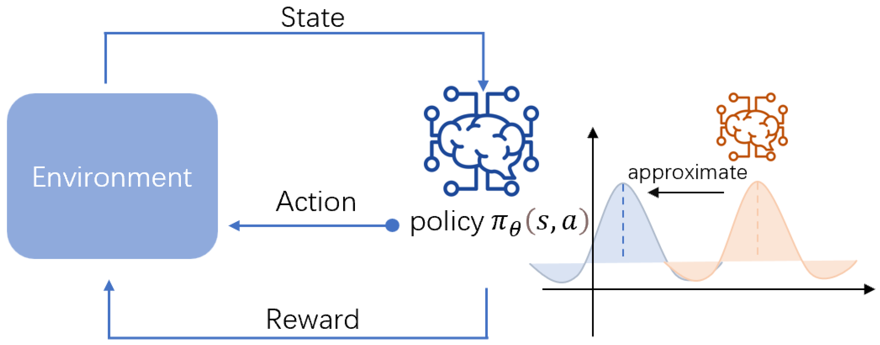
The goal is to adjust the parameters of the student model so that its policy distribution closely approximates the teacher model’s policy distribution. The pseudocode is shown in Algorithm 2 and the illustration is shown in Figure 3.
| Algorithm 2 Policy distillation process. |
|
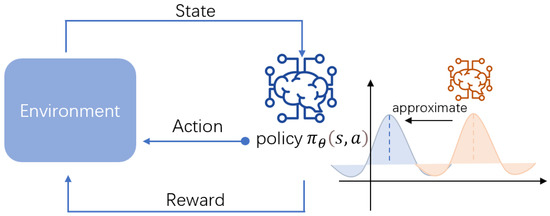
Figure 3.
Representation of policy distillation process.
4.3. Teacher and Assistant
Generally, students typically receive guidance from a single teacher, and single-teacher policy distillation can also transfer the optimal policy to the student model, achieving satisfactory accuracy. However, if the teacher’s teaching style or method does not suit a particular student, that student may not achieve ideal learning outcomes. Some researchers have also suggested that learning from a single teacher may introduce inductive bias. That is, the teacher model may perform inadequately in certain environments due to reasons inherent to the model itself or insufficient training [5]. Based on this consideration, we introduce an assistant model in the RAN slicing environment as a supplement, proposing a dual-model policy distillation with both teacher and assistant models.
This approach offers multiple advantages. Firstly, the assistant model provides additional support, overcoming the limitations of a single teacher model, ensuring the robustness and reliability of the student model in variable environments. Secondly, the assistant model can offer valuable feedback to the student model, enabling faster adjustment and optimization of strategies. This enhanced adaptability is particularly critical in dynamically changing RAN environments, allowing the student model to quickly converge to the optimal strategy. Consequently, it improves response speed and efficiency in slices with adjusted SLA weights, thereby enhancing the QoE for users in RAN slicing.
Specifically, for slices with changing SLA weights (referred to as Student Slices), we first use cosine similarity to match the two most similar pre-trained models. Then, based on the performance of these two models under the new slice weight configuration, we designate them as the teacher and assistant for policy distillation. We initially set the base weights of the teacher and assistant models to 0.8 and 0.2, respectively. Then, based on their performance on the student slices, we dynamically adjust their weights to better meet the actual requirements.The teacher model is typically more stable and reliable in performance, providing more accurate and effective guidance, thus occupying the main proportion. The assistant model, serving as a supplementary role, provides additional support and validation, ensuring that valuable information is still provided to the student model even if the teacher model performs inadequately.
Due to the ability to share the teacher and assistant models, a high level of accuracy has been achieved, the need for pre-trained slice models is significantly reduced, requiring only eight models to be maintained. The intuition behind choosing these models is that they are evenly distributed and as far from the vertices as possible on the unit simplex in three-dimensional space. Secondly, they should have the smallest possible cosine similarity values with all subsequent student slice weight vectors. These models achieve a good balance between optimizing the number of models and maintaining accuracy, reducing the number of teacher models that need to be maintained while ensuring that the subsequent student models are as similar as possible to the matched teacher models. This ensures the accuracy of policy transfer, significantly enhancing the real-time response capability of the RAN slicing.
The TADocs dual-model policy distillation method optimizes the matching process, effectively overcoming the limitations of a single model and providing a more robust and reliable solution.
4.4. Algorithm Complexity
The primary computational cost of TADocs arises from training using the PPO algorithm in the 6G network slicing reinforcement learning environment. Therefore, we analyze it in terms of both time complexity and space complexity.
4.4.1. Time Complexity
The time complexity is primarily determined by the following factors:
Number of policy updates (N): PPO requires multiple gradient descent steps for each policy update. Therefore, its complexity depends on the number of updates.
Batch size (B): PPO typically optimizes over batches of data. The larger the batch size, the more time is required for each update.
Feature dimension (d): The complexity of the policy network is influenced by the dimensionality of the feature space. If neural networks are used, the complexity of forward and backward propagation depends on the number of layers and neurons in the network.
The overall time complexity of PPO can be expressed as:
where: N is the number of policy updates, B is the batch size, d is the feature dimension.
4.4.2. Space Complexity
The space complexity of PPO depends on two key factors:
Model parameters: PPO’s policy and value networks are usually deep neural networks, and the number of model parameters depends on the depth of the network and the number of neurons per layer.
Experience storage: PPO stores trajectories, including states, actions, rewards, and value estimates. Therefore, the space complexity is proportional to the number of stored experiences and the size of each sample.
The overall space complexity can be expressed as:
where: P is the number of model parameters, T is the length of stored trajectories, d is the dimension of the state or feature.
5. Experiments
5.1. Environment Setup
The programs used in this study were run on a high-performance AI server equipped with dual Intel® Xeon® Silver 4309Y CPUs @ 2.80 GHz and dual NVIDIA RTX 4090 GPUs, with 128 GB of RAM, running Ubuntu 22.04. All simulation experiments were implemented in Python 3.8.18. The PPO deep reinforcement learning algorithm was employed using the open-source library stable-baselines3 (available at https://github.com/DLR-RM/stable-baselines3, accessed on 18 June 2024). The experiments were conducted using a simulated reinforcement learning environment based on RAN slicing, which is available on GitHub (Available at https://github.com/ahmadnagib/TL4RL, accessed on 18 June 2024). This environment was extended from the widely recognized Gymnasium framework. In the simulation environment, three types of network slices were defined: VoLTE, uRLLC, and video. To make the simulation more realistic, we used three different probability distribution models to simulate these service types. Specifically, VoLTE traffic was generated using a uniform distribution, uRLLC traffic was simulated using an exponential distribution, and video traffic was generated using a truncated Pareto distribution. The parameters for the inter-packet intervals and packet size distributions for each service type are detailed in Table 3.

Table 3.
Scheduling and generation methods for RAN slicing services.
During the experiments, we created a queue containing 400,000 service requests and instructed the reinforcement learning agent to handle the requests using a round-robin (RR) scheduling strategy. In reinforcement learning, to motivate the agent to process tasks efficiently, the reward function is designed to be an inverse form of the total service processing time. Through training, the agent can learn the optimal strategy under the given slice weight configuration to process accumulated service requests in the shortest possible time.
Apart from the aforementioned eight pre-trained models, we also selected ten randomly generated student slice models for the experiments to simulate the slice weight configuration parameters after changes in the SLA. During the selection process, we conducted a comprehensive search over the interval and generated weights, ensuring that student slice models were selected in each segment of the interval. This method ensures that even weights with low probability have a chance of being selected, maximizing the fairness of the experiment. Detailed information about these model weights can be found in Table 4.

Table 4.
Weights of teachers and students.
5.2. Experimental Process
To ensure the fairness of the experimental results, each set of experimental conditions was run independently five times, and the mean value was used as the final measurement. This repeated experimental approach helps reduce the impact of random errors and enhances the statistical reliability of the experimental conclusions.
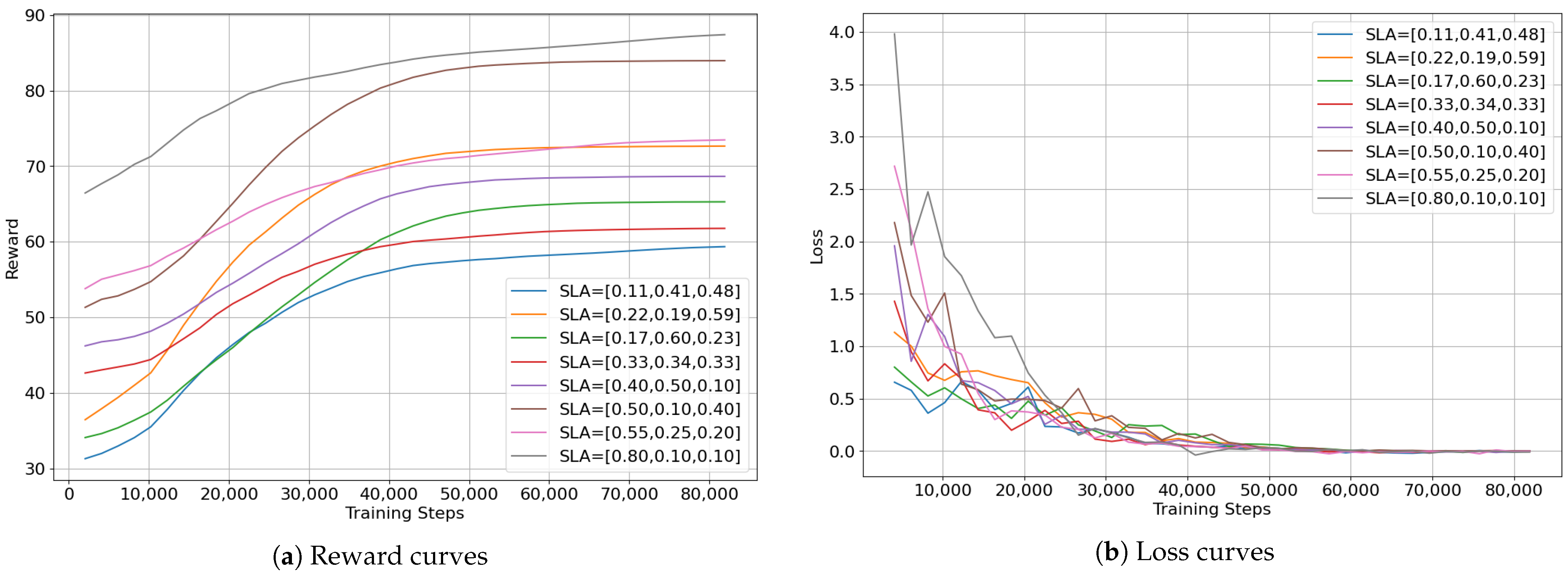
The experimental environment integrated Stable Baselines3, which facilitates access to various reinforcement learning algorithms. We selected the Proximal Policy Optimization (PPO) algorithm as the core training mechanism. Due to its outstanding stability and efficiency, the PPO algorithm was chosen as the preferred solution for training and optimizing the reinforcement learning models, ensuring the robustness and accuracy of the experimental results. The PPO algorithm was applied to train the eight teacher models; the hyperparameter settings used for training are detailed in Table 5. For each teacher model, after 80,000 steps of training, the reward curves and loss curves during the training process are shown in Figure 4a,b, respectively. These curves indicate that the eight models have been fully trained and have converged.

Table 5.
PPO algorithm parameters.
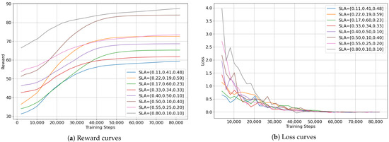
Figure 4.
Training and loss curves of teacher models trained using PPO.
Through the experiments, we aim to compare the differences between the TADocs method, the single-teacher strategy distillation, and the direct training results using PPO, to demonstrate the significant advantages of TADocs in terms of time consumption, accuracy, and stability.
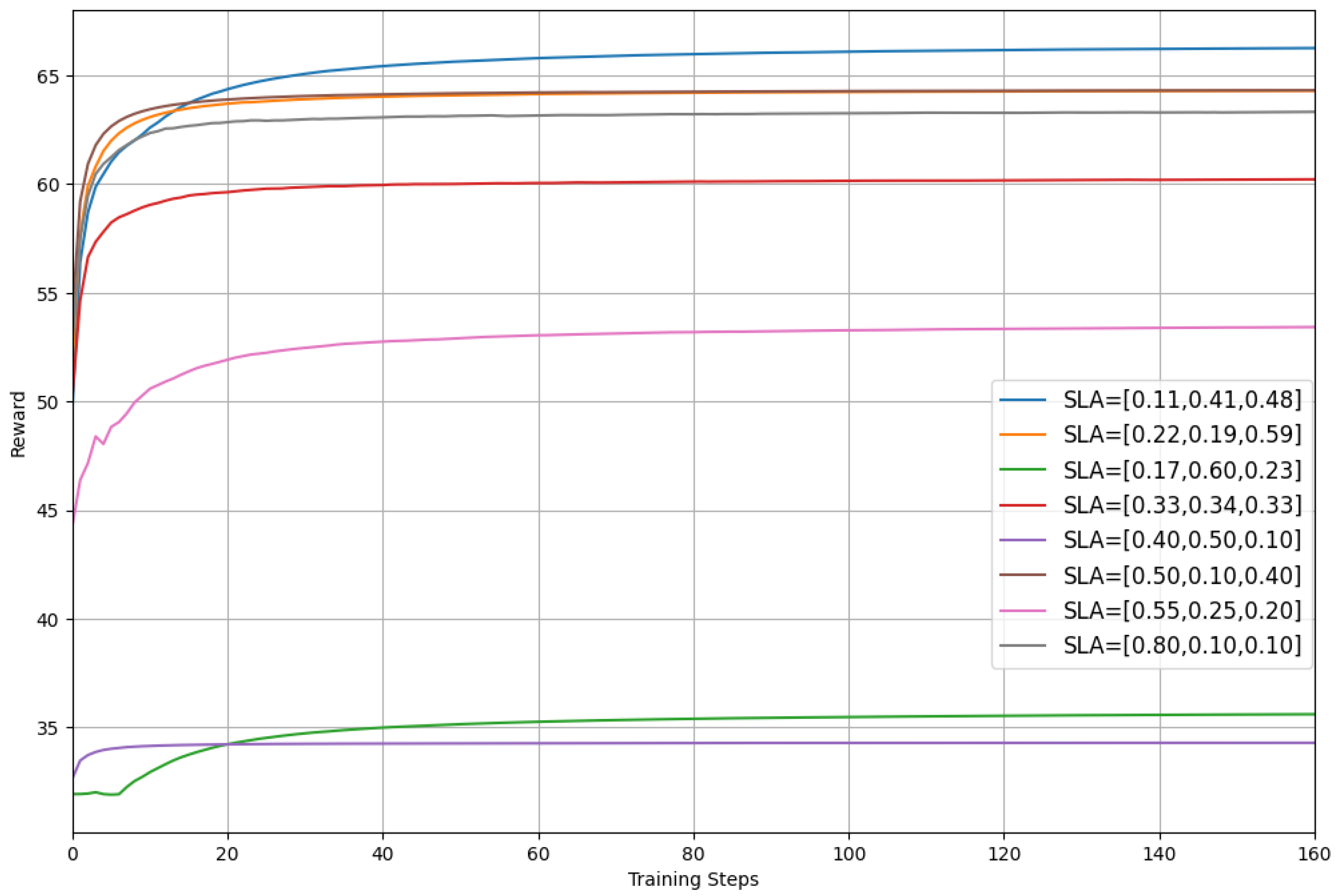
We first randomly selected a student network slice model and then used the eight different teacher models mentioned above to perform policy distillation. As shown in Figure 5, the results reveal significant differences in the effects produced by different teacher models during the distillation process. This phenomenon indicates that choosing an appropriate learning object for targeted teaching is extremely important. A suitable teacher model can not only effectively transfer knowledge but can also help the student model achieve a better performance in specific tasks. Therefore, in the process of policy distillation, selecting the appropriate teacher model is a crucial factor in enhancing the learning effectiveness of the student model.
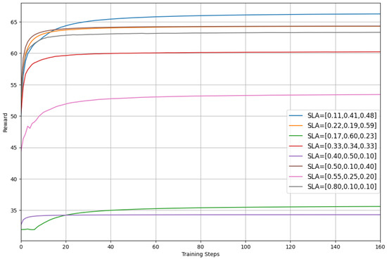
Figure 5.
The reward for policy distillation using different teacher models.
5.3. Experimental Results
We compared the training time for 10 student slice models between the PPO and the TADocs. When the SLA weights changed, the average time taken using the TADocs method was 238.82 s, while the average time taken using the PPO algorithm was 1253.12 s. This indicates that the TADocs method significantly reduced the time cost, decreasing the training time by approximately 81%, as shown in Figure 6.
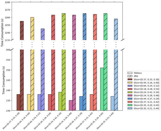
Figure 6.
Comparison of Time Consumption of PPO and TADocs.
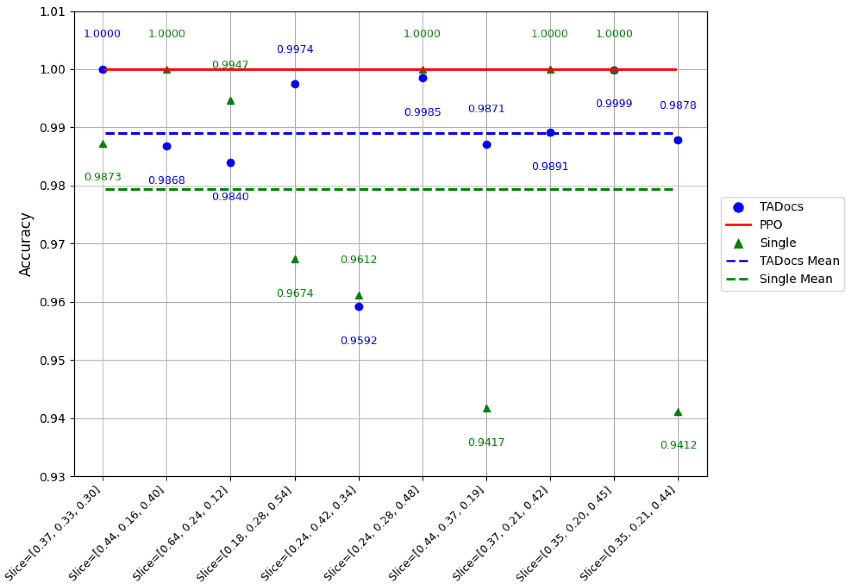
In terms of accuracy, we defined the accuracy obtained by training with the PPO algorithm as 100%. Using TADocs, we achieved an average accuracy of 98.96%, which is very close to the accuracy obtained through training from scratch. This demonstrates that the TADocs method can maintain a high level of performance while significantly reducing training time. This result further proves the effectiveness of the TADocs method in practical applications; not only does it significantly reduce time costs but it also provides accuracy comparable to traditional methods, as shown in Figure 7.
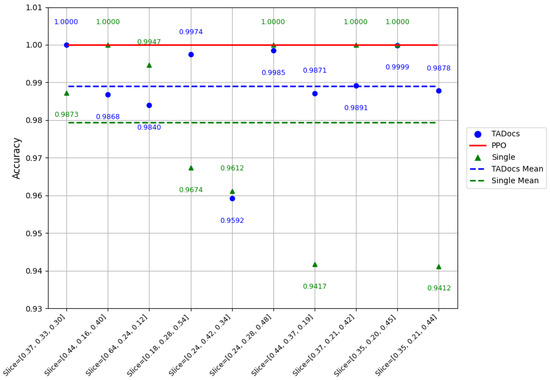
Figure 7.
Comparison of accuracy and stability between PPO, TADocs, and single teacher.
It is important to note that we experimentally verified that the TADocs method works effectively across heterogeneous models as well. Considering that reinforcement learning models are usually small—for example, a standard PPO model typically contains two or three hidden layers, with each layer consisting of 64–256 hidden units—such models have tens of thousands to hundreds of thousands of trainable parameters. The specific number of parameters varies depending on the dimensions of the state space and action space. We verified that the TADocs method performs well in terms of accuracy when distilling the policy into a smaller model. Our experiments primarily explored the effectiveness of the TADocs method in policy transfer. Although the above characteristics show potential in scenarios involving model compression and resource constraints, this paper does not discuss the results in detail.
5.4. Ablation Study
Finally, we performed essential ablation experiments.
In Ablation Experiment 1, we used single-teacher-to-single-student policy distillation. The experimental results showed that policy distillation using a single-teacher model was approximately 1% lower in average accuracy compared to the TADocs method.
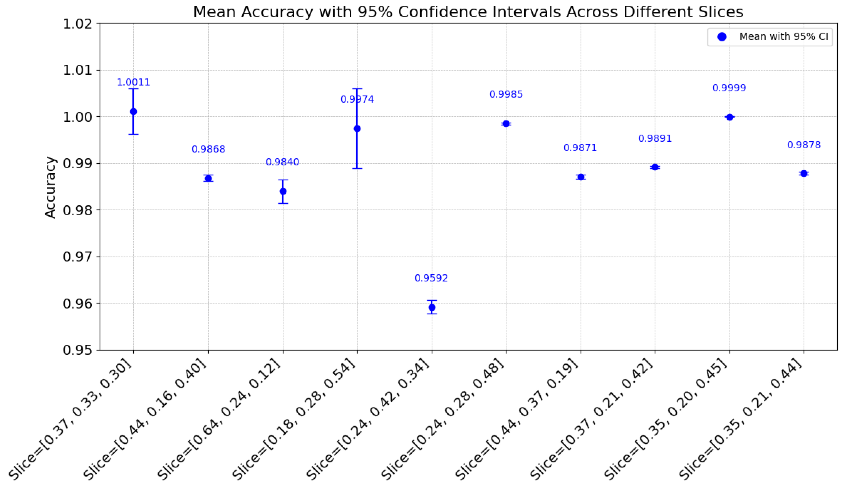
To ensure the reliability of the experimental results, we conducted a 95% confidence interval experiment. This experiment allowed us to more accurately assess the stability and performance of the model. The results presented in Figure 8 display the range of the data along with the confidence level. The 95% confidence interval indicates that we are 95% confident that the true value lies within this interval, which further strengthens the credibility and robustness of the experimental findings. This experiment not only provides statistical support for the results but also helps us better understand the variations in the model’s performance under different conditions.

Figure 8.
Mean accuracy with 95% confidence intervals across different slices.
In terms of stability, the TADocs method also demonstrated significant advantages. As shown in Figure 7, the lowest accuracy achieved by single-teacher policy distillation was only 94.12%, whereas the TADocs method maintained an accuracy of 95.92% even in the most unfavorable conditions. Moreover, from the figure, we can see that the stability of the curves for the TADocs method is significantly better than that of the single-teacher to single-student policy distillation.
These results indicate that the TADocs method has significant advantages in terms of both the accuracy and stability of the training results. Specifically, the TADocs method enhances the efficiency and effectiveness of policy transfer by introducing the collaborative effect of multiple teachers and assistants, allowing the student model to benefit from richer and more diverse knowledge.
In Ablation Experiment 2, we further validated the previous conclusion that using cosine similarity for matching is more accurate than using Euclidean distance. Specifically, cosine similarity demonstrated higher accuracy and greater stability in the vast majority of scenarios.
From Table 6, it is evident that for certain student slices, the most suitable teacher models identified using Euclidean distance and cosine similarity differ. When these models are employed for policy distillation, allowing the student slice models to learn from them, the learning outcomes exhibit significant differences. This underscores the importance of selecting appropriate learning targets. The experimental data in the table allow for further analysis and the validation of this conclusion.

Table 6.
Comparison of cosine similarity and Euclidean distance.
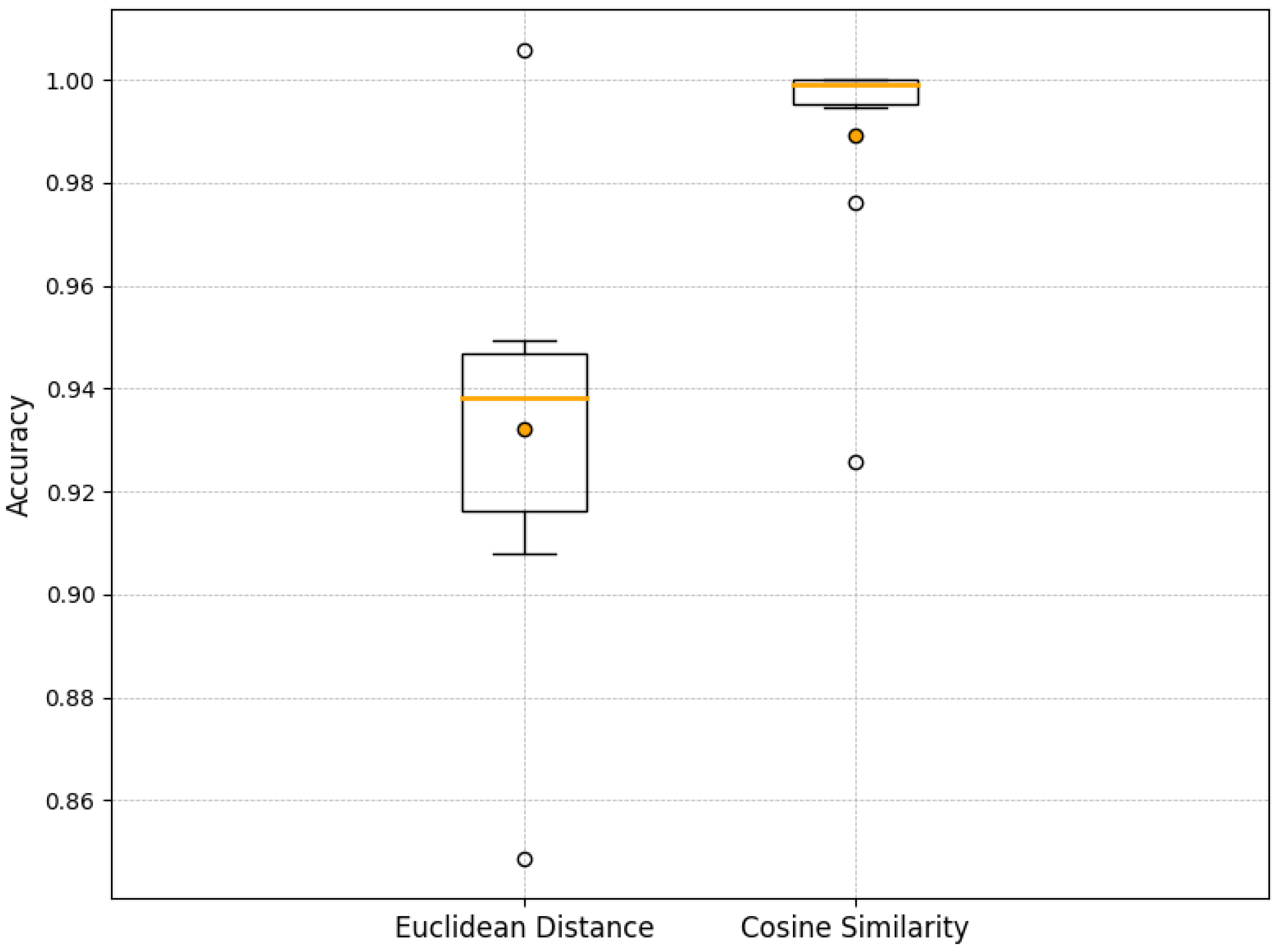
As shown in Figure 9, the yellow bars represent the matching accuracy calculated using Euclidean distance. It can be seen from the figure that the matching accuracy using cosine similarity is generally higher and more stable, with numerous data points having an accuracy close to or equal to 1.0. This indicates that cosine similarity better captures the similarity between data, allowing the model to more accurately select teachers and assistants during matching, thereby improving the learning efficiency of policy transfer. In contrast, the matching accuracy using Euclidean distance shows greater variance. This suggests that Euclidean distance may be less reliable in certain situations. Euclidean distance primarily measures the absolute distance between vectors, which can be influenced by the scale of the vectors, making its performance potentially less stable when dealing with data of different scales.
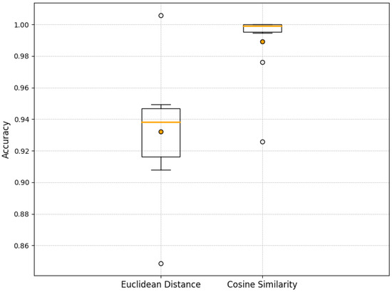
Figure 9.
Comparison of accuracy and stability between matching using Ccsine similarity and Euclidean distance.
In summary, cosine similarity demonstrates higher accuracy and stability in matching tasks, while Euclidean distance shows a wider range of accuracy fluctuations. This stability is particularly important in RAN slicing scenarios, as it ensures that the student model performs excellently under various new SLA weight parameter conditions, thereby improving the QoE for users.
6. Discussion
The TADocs method adopts cosine similarity as the standard for matching the most suitable teacher models, significantly enhancing matching accuracy compared to other methods. This lays a solid foundation for subsequent policy distillation. Additionally, the introduction of the assistant mechanism mitigates model inductive bias to some extent. Experimental results further demonstrate that the TADocs method significantly reduces convergence time while maintaining high accuracy. Moreover, this method excels in the transfer of policy knowledge between heterogeneous models, which holds significant practical relevance, especially in applications such as model compression in edge networks.
In future research, we will continue to explore the application of the TADocs method to more complex tasks to further enhance its practical value. We also plan to reduce the number of pre-trained models and conduct an in-depth investigation into the intrinsic relationships of agent behavior under different slice weight environments. Furthermore, we will consider adopting a meta-learning framework, such as a meta-weight network, to study and establish dynamic mappings between different slices and agents. This approach aims to effectively perform policy distillation under arbitrary RAN slice weight parameters using fewer teacher models, thereby further improving the efficiency and practicality of the solution in similar scenarios.
7. Conclusions
This paper addresses a key practical challenge in deploying RL-based resource management solutions in dynamic wireless network environments. In the O-RAN scenario, MNOs often adjust the priority of available network slices’ SLA, which leads to the need for RL agents to be retrained, resulting in excessively long convergence times. To address this, we propose the TADocs method and validate its effectiveness through comprehensive experiments. We model the slices with modified SLA as student models and use cosine similarity as a metric to find the most appropriate teacher and assistant models. Subsequently, through policy distillation in reinforcement learning, the student model learns from the teacher and assistant models, achieving fast convergence and high performance. Experimental results show that the TADocs method demonstrates significant superiority in policy distillation, particularly in the collaborative role of the teacher and assistant models, which enhances model performance and stability. Specifically, with TADocs, the agents’ convergence time is reduced by 81%, while maintaining an average accuracy of over 98%. This marks an important step towards intelligent resource management in O-RAN, significantly improving MNOs’ operational efficiency while enhancing the quality of experience for users. We believe that reinforcement learning methods based on policy distillation have the potential to become commercial solutions and demonstrate promising applications in the future.
Author Contributions
X.M.: Conceptualization, Methodology, Writing—Original Draft Preparation. Y.X.: Investigation. D.L.: Supervision and Reviewing. M.L.: Validation. All authors have read and agreed to the published version of the manuscript.
Funding
This work was supported by National Key R&D Program of China (2019YFB1804400), Science and Technology Development Fund (FDCT) of Macau under Grant 0095/2023/RIA2, and the Chinese Society of Educational Development Strategy (ZLB20240823).
Data Availability Statement
The data are available from the corresponding author on reasonable request.
Conflicts of Interest
The authors declare no conflicts of interest.
Abbreviations
The following abbreviations are used in this manuscript:
| O-RAN | Open Radio Access Network |
| MNOs | Mobile Network Operators |
| TTI | Transmission Time Interval |
| SLA | Service Level Agreement |
| QoE | Quality of Experience |
| QoS | Quality of Service |
| RR | Round-Robin |
| Resource allocation vector | |
| Total system resources | |
| Bandwidth resources allocated to the i-th slice | |
| Minimum bandwidth requirement of the i-th slice | |
| Delay of the i-th slice | |
| Maximum acceptable delay of the i-th slice | |
| Packet loss rate of the i-th slice | |
| Maximum acceptable packet loss rate of the i-th slice | |
| Environment | |
| State at time t | |
| Optimal policy | |
| Reward at time step t | |
| Discount factor | |
| State vector | |
| Importance of delay time for each slice | |
| L | Reciprocal of the available slice delay |
| Policy distribution of the teacher model | |
| Policy distribution of the student model |
References
- Afolabi, I.; Taleb, T.; Samdanis, K.; Ksentini, A.; Flinck, H. Network slicing and softwarization: A survey on principles, enabling technologies, and solutions. IEEE Commun. Surv. Tutor. 2018, 20, 2429–2453. [Google Scholar] [CrossRef]
- Wang, J.; Zhao, L.; Liu, J.; Chen, Y.; Kwak, K.S. Smart resource allocation for mobile edge computing: A deep reinforcement learning approach. IEEE Trans. Emerg. Top. Comput. 2019, 9, 1529–1541. [Google Scholar] [CrossRef]
- Li, R.; Yuan, H.; Ren, B.; Zhang, X.; Chen, T.; Luo, X. When Optimization Meets AI: An Intelligent Approach for Network Disintegration with Discrete Resource Allocation. Mathematics 2024, 12, 1252. [Google Scholar] [CrossRef]
- Hinton, G.; Vinyals, O.; Dean, J. Distilling the knowledge in a neural network. arXiv 2015, arXiv:1503.02531. [Google Scholar]
- Ren, S.; Gao, Z.; Hua, T.; Xue, Z.; Tian, Y.; He, S.; Zhao, H. Co-advise: Cross inductive bias distillation. In Proceedings of the IEEE/CVF Conference on Computer Vision and Pattern Recognition, New Orleans, LA, USA, 18–24 June 2022; pp. 16773–16782. [Google Scholar]
- Suh, K.; Kim, S.; Ahn, Y.; Kim, S.; Ju, H.; Shim, B. Deep reinforcement learning-based network slicing for beyond 5G. IEEE Access 2022, 10, 7384–7395. [Google Scholar] [CrossRef]
- Kim, Y.; Kim, S.; Lim, H. Reinforcement learning based resource management for network slicing. Appl. Sci. 2019, 9, 2361. [Google Scholar] [CrossRef]
- Kanellopoulos, D.; Sharma, V.K. Dynamic load balancing techniques in the IoT: A review. Symmetry 2022, 14, 2554. [Google Scholar] [CrossRef]
- Celdrán, A.H.; Pérez, M.G.; Clemente, F.J.G.; Ippoliti, F.; Pérez, G.M. Policy-based network slicing management for future mobile communications. In Proceedings of the 2018 Fifth International Conference on Software Defined Systems (SDS), Barcelona, Spain, 23–26 April 2018; pp. 153–159. [Google Scholar]
- Guan, W.; Zhang, H.; Leung, V.C.M. Customized slicing for 6G: Enforcing artificial intelligence on resource management. IEEE Netw. 2021, 35, 264–271. [Google Scholar] [CrossRef]
- Zhao, N.; Liang, Y.C.; Niyato, D.; Pei, Y.; Wu, M.; Jiang, Y. Deep reinforcement learning for user association and resource allocation in heterogeneous cellular networks. IEEE Trans. Wirel. Commun. 2019, 18, 5141–5152. [Google Scholar] [CrossRef]
- Villota-Jacome, W.F.; Rendon, O.M.C.; da Fonseca, N.L.S. Admission control for 5G core network slicing based on deep reinforcement learning. IEEE Syst. J. 2022, 16, 4686–4697. [Google Scholar] [CrossRef]
- Xie, Y.; Kong, Y.; Huang, L.; Wang, S.; Xu, S.; Wang, X.; Ren, J. Resource allocation for network slicing in dynamic multi-tenant networks: A deep reinforcement learning approach. Comput. Commun. 2022, 195, 476–487. [Google Scholar] [CrossRef]
- Huang, Z.; Li, D.; Cai, J.; Lu, H. Collective reinforcement learning based resource allocation for digital twin service in 6G networks. J. Netw. Comput. Appl. 2023, 217, 103697. [Google Scholar] [CrossRef]
- Wang, H.; Wu, Y.; Min, G.; Xu, J.; Tang, P. Data-driven dynamic resource scheduling for network slicing: A deep reinforcement learning approach. Inf. Sci. 2019, 498, 106–116. [Google Scholar] [CrossRef]
- Zhu, Z.; Lin, K.; Jain, A.K.; Zhou, J. Transfer learning in deep reinforcement learning: A survey. IEEE Trans. Pattern Anal. Mach. Intell. 2023, 45, 13344–13362. [Google Scholar] [CrossRef] [PubMed]
- Hieu, N.Q.; Hoang, D.T.; Niyato, D.; Wang, P.; Kim, D.I.; Yuen, C. Transferable deep reinforcement learning framework for autonomous vehicles with joint radar-data communications. IEEE Trans. Commun. 2022, 70, 5164–5180. [Google Scholar] [CrossRef]
- Rusu, A.A.; Colmenarejo, S.G.; Gulcehre, C.; Desjardins, G.; Kirkpatrick, J.; Pascanu, R.; Mnih, V.; Kavukcuoglu, K.; Hadsell, R. Policy distillation. arXiv 2015, arXiv:1511.06295. [Google Scholar]
- Jang, I.; Kim, H.; Lee, D.; Son, Y.S.; Kim, S. Knowledge transfer for on-device deep reinforcement learning in resource constrained edge computing systems. IEEE Access 2020, 8, 146588–146597. [Google Scholar] [CrossRef]
- Yuan, F.; Shou, L.; Pei, J.; Lin, W.; Gong, M.; Fu, Y.; Jiang, D. Reinforced multi-teacher selection for knowledge distillation. Proc. AAAI Conf. Artif. Intell. 2021, 35, 14284–14291. [Google Scholar] [CrossRef]
- Zhang, H.; Chen, D.; Wang, C. Confidence-aware multi-teacher knowledge distillation. In Proceedings of the ICASSP 2022–2022 IEEE International Conference on Acoustics, Speech and Signal Processing (ICASSP), Singapore, 23–27 May 2022; pp. 4498–4502. [Google Scholar]
- Nagib, A.M.; Abou-Zeid, H.; Hassanein, H.S. Accelerating reinforcement learning via predictive policy transfer in 6G RAN slicing. IEEE Trans. Netw. Serv. Manag. 2023, 20, 1170–1183. [Google Scholar] [CrossRef]
- Kanellopoulos, D.; Sharma, V.K.; Panagiotakopoulos, T.; Kameas, A. Networking architectures and protocols for IoT applications in smart cities: Recent developments and perspectives. Electronics 2023, 12, 2490. [Google Scholar] [CrossRef]
- Dulac-Arnold, G.; Levine, N.; Mankowitz, D.J.; Li, J.; Paduraru, C.; Gowal, S.; Hester, T. Challenges of real-world reinforcement learning: Definitions, benchmarks and analysis. Mach. Learn. 2021, 110, 2419–2468. [Google Scholar] [CrossRef]
- Trienekens, J.J.M.; Bouman, J.J.; Van Der Zwan, M. Specification of service level agreements: Problems, principles and practices. Softw. Qual. J. 2004, 12, 43–57. [Google Scholar] [CrossRef]
- Chergui, H.; Blanco, L.; Garrido, L.A.; Ramantas, K.; Kukliński, S.; Ksentini, A.; Verikoukis, C. Zero-touch AI-driven distributed management for energy-efficient 6G massive network slicing. IEEE Netw. 2021, 35, 43–49. [Google Scholar] [CrossRef]
Disclaimer/Publisher’s Note: The statements, opinions and data contained in all publications are solely those of the individual author(s) and contributor(s) and not of MDPI and/or the editor(s). MDPI and/or the editor(s) disclaim responsibility for any injury to people or property resulting from any ideas, methods, instructions or products referred to in the content. |
© 2024 by the authors. Licensee MDPI, Basel, Switzerland. This article is an open access article distributed under the terms and conditions of the Creative Commons Attribution (CC BY) license (https://creativecommons.org/licenses/by/4.0/).

