Non-Linear Plasma Wave Dynamics: Investigating Chaos in Dynamical Systems

Abstract

This work addresses the significant issue of plasma waves interacting with non-linear dynamical systems in both perturbed and unperturbed states, as modeled by the generalized Whitham–Broer–Kaup–Boussinesq–Kupershmidt (WBK-BK) Equations. We investigate analytical solutions and the subsequent emergence of chaos within these systems. Initially, we apply advanced mathematical techniques, including the transform method and the ${\displaystyle \frac{G^{\prime }}{G^2}}$ method. These methods allow us to derive new precise solutions and enhance our understanding of the non-linear processes dominating plasma wave dynamics. Through a systematic analysis, we identify the conditions under which the system transitions from orderly patterns to chaotic behavior. This investigation provides valuable insights into the fundamental mechanisms of non-linear wave propagation in plasmas. Our results highlight the dynamic interplay between non-linearity and variation, leading to chaos, which may be useful in predicting and potentially controlling similar phenomena in practical applications.

1. Introduction

Plasma waves, a fascinating aspect of plasma physics, present significant theoretical and applied challenges to scientists due to cyclically occurring resonances, non-linear interactions, and suppression of waves that emerge in space plasmas [1,2]. This paper examines the derivation of the generalized Whitham–Broer–Kaup–Boussinesq–Kupershmidt (WBK-BK) wave dynamics [3]. These equations serve as robust models describing the intricate behavior of non-linear dynamical systems in both perturbed and unperturbed states [4,5,6,7]. By analyzing the WBK-BK equations, we aim to uncover new solutions and mechanisms that highlight the complexity of wave dynamics in plasma systems.

The Whitham–Broer–Kaup, Boussinesq, and Kupershmidt equations have long been demonstrated to accurately represent wave propagation in various types of motion, such as turbulence in fluids or plasmas [8,9]. These equations encapsulate the intricate interplay of non-linearity and dispersion, two key components underlying the formation and evolution of soliton–stationary localized wave packets that maintain their form over time and space [10,11,12]. In the context of plasma waves, these solutions provide critical insights into the stability and behavior of plasmonic systems.

Our investigation into the WBK-BK equations is driven by the goal of finding exact solutions and determining the boundaries of the system’s chaotic behavior. The transition from regular and predictable dynamics to unpredictable and chaotic ones is a fundamental characteristic of complex systems [13,14], and it significantly impacts wave propagation and stability in plasma physics [5]. Understanding these transitions is crucial for both theoretical studies and practical applications, including laboratory studies on controlled fusion and experiments with space plasmas.

Perhaps the most significant PDEs are the generalized WBK–BK equations. This paper examines the WBK-BK equations in the following ways [3]:

$$\left\{\begin{array}{c}{\displaystyle \frac{\partial \mathsf{\Phi }}{\partial \eta }}+\kappa \varphi {\displaystyle \frac{\partial \mathsf{\Phi }}{\partial \chi }}+\kappa {\displaystyle \frac{\partial \omega }{\partial \chi }}+m{\displaystyle \frac{{\partial }^2\mathsf{\Phi }}{\partial {\chi }^2}}=0,\hfill \\ {\displaystyle \frac{\partial \omega }{\partial \eta }}+\kappa \varphi {\displaystyle \frac{\partial \omega }{\partial \chi }}+\kappa \omega {\displaystyle \frac{\partial \varphi }{\partial \chi }}+\rho {\displaystyle \frac{{\partial }^3\mathsf{\Phi }}{\partial {\chi }^3}}-m{\displaystyle \frac{{\partial }^2\omega }{\partial {\chi }^2}}=0.\hfill \end{array}\right.$$

(1)

The term $\varphi =\varphi (\eta ,\chi )$ represents the horizontal velocity of the wave, while $\omega =\omega (\eta ,\chi )$ indicates the wave’s deviation from its equilibrium position. Real constants $\kappa$, m, and $\rho$ correspond to various diffusion scenarios. A time-like or extra spatial variable influencing the system’s evolution is probably indicated by $\eta$, whilst the main spatial coordinate that the dynamics of the fields $\mathsf{\Omega }$ and $\omega$ are examined along is represented by $\chi$. In [3], Oloniiju employed the sine-Gordon expansion method to study the soliton solutions of Equation (1). The primary objective of this paper is to examine the dynamic behavior of Equation (1) and discover novel soliton solutions.

To achieve our goals, we utilize a collection of advanced mathematical techniques, including the change of variables method and the ${\displaystyle \frac{G^{\prime }}{G^2}}$-method. These approaches allow us to find exact solutions for non-linear differential equations that were previously unknown, thereby broadening our understanding of the non-linear behavior of these phenomena [15,16]. Specifically, the ${\displaystyle \frac{G^{\prime }}{G}}$-method simplifies complex non-linear equations, facilitating the discovery of exact solutions [17].

Our results suggest the presence of a boring-in effect along with wave anomalies in plasma wave dynamics. This is achieved through a systematic study of the exact solutions obtained via these methods, enabling us to identify the conditions under which the systems transition from stable to chaotic modes [9,18,19]. These phenomena result from the transition from order to chaos, characterized by a combination of randomness and the existence of strange attractors in phase space. Furthermore, our research provides valuable theoretical perspectives and practical methods for predicting and controlling similar chaotic behavioral patterns in physical systems. By understanding the mechanisms that lead to chaos, we can potentially mitigate its adverse effects or even utilize it for practical applications. For instance, in wave systems, maintaining stability during plasma wave generation is crucial for the controlled release of fusion energy.

In summary, this study presents the behavior of plasma waves using the WBK-BK equations. By finding exact solutions and examining the necessary conditions for the emergence of chaos, we contribute to a broader understanding of non-linearity in wave propagation and stability in plasma physics [16,20,21]. The results confirm the highly complex relationship between non-linearity and perturbations. Consequently, our findings provide valuable information and potential applications in fields where wave dynamics are critical, such as engineering and oceanography. This work illustrates how the ${\displaystyle \frac{G^{\prime }}{G^2}}$ technique can be used to develop closed-form solutions for wave equations exhibiting solitary behavior. The WBK-BK equation family is explored to ascertain the method’s suitability, and we also propose some new ideas. We apply this technique to solitary waves, kink-type modes, and plasma waves to achieve plausible wavelengths. The absolute value limit is considered during the process. This method excels in its simplicity and computational efficiency, making it ideal for various applications, including those that require handling evolved genetic statistics offline. The clarity and effectiveness of the ${\displaystyle \frac{G^{\prime }}{G^2}}$ method make it a promising tool for future studies aimed at improving the treatment of diseases and solving complex problems in theoretical physics, practical mathematics, and non-linear sciences and engineering. Finally, we present graphical representations of the chaotic movement of non-linearly stable waves, considering singularities and bifurcations. The conclusions of this paper will be discussed in the last section.

2. Mathematical Model

2.1. Description of Methods

First, attention is given to the wave change:

$$H\left(\varphi ,{\varphi }_{\chi },{\varphi }_{\eta },{\varphi }_{\chi \chi },{\varphi }_{\eta \eta },\dots \right)=0,$$

(2)

where $\varphi \left(\chi ,\eta \right)$ is an unknown function and H is a polynomial in $\varphi$. Thus, the transmutation method is used to obtain to the plasma wave solution.

$$\begin{array}{c}\hfill \varphi \left(\chi ,\eta \right)=\mathsf{\Phi }\left(\xi \right),\omega \left(\chi ,\eta \right)=\mathsf{\Omega }\left(\xi \right),\xi =\chi +\sigma \eta ,\end{array}$$

(3)

where ‘$\xi$’ is the amplitude of the wave and ‘$\sigma$’ represents the speed. We apply the aforementioned transformation to Equation (1) to convert it into a non-linear ODE.

$$F\left(\mathsf{\Phi },{\mathsf{\Phi }}^{\prime },{\mathsf{\Phi }}^{″},\dots \right)=0,$$

(4)

where F represents a polynomial and ${\mathsf{\Phi }}^{\prime }={\displaystyle \frac{d\mathsf{\Phi }}{d\xi }}$, ${\mathsf{\Phi }}^{″}={\displaystyle \frac{d^2\mathsf{\Phi }}{d{\xi }^2}}$ and so on are its derivatives.

$$\sigma {\mathsf{\Phi }}^{\prime }+\kappa \mathsf{\Phi }{\mathsf{\Phi }}^{\prime }+\kappa {\mathsf{\Omega }}^{\prime }+m{\mathsf{\Phi }}^{″}=0.$$

(5)

$$\sigma {\mathsf{\Omega }}^{\prime }+\kappa \mathsf{\Phi }{\mathsf{\Omega }}^{\prime }+\kappa \mathsf{\Omega }{\mathsf{\Phi }}^{\prime }+\rho {\mathsf{\Phi }}^{‴}-m{\mathsf{\Omega }}^{″}=0.$$

(6)

On integrating Equation (5) w.r.t ‘$\xi$’, we obtain:

$$\mathsf{\Omega }\left(\xi \right)=-{\displaystyle \frac{\sigma }{\kappa }}\mathsf{\Phi }-{\displaystyle \frac{1}{2}}{\mathsf{\Phi }}^2-{\displaystyle \frac{m}{\kappa }}{\mathsf{\Phi }}^{\prime },$$

(7)

and by substituting the valve of Equation (7) into Equation (6), we obtain:

$${\mathsf{\Phi }}^{″}={\displaystyle \frac{{\kappa }^2}{2(m^2+\rho \kappa )}}{\mathsf{\Phi }}^3+{\displaystyle \frac{3\sigma \kappa }{2(m^2+\rho \kappa )}}{\mathsf{\Phi }}^2+{\displaystyle \frac{{\sigma }^2}{2(m^2+\rho \kappa )}}\mathsf{\Phi }+{\displaystyle \frac{C\kappa }{2(m^2+\rho \kappa )}},$$

(8)

where ‘C’ is the integral constant in this case.

We suppose that Equation (4) has a form of solution as mentioned below:

$$\mathsf{\Phi }\left(\xi \right)=m_0+m_1\left({\displaystyle \frac{G^{\prime }}{G^2}}\right).$$

(9)

2.2. The Extended $\left({\displaystyle \frac{G^{\prime }}{G^2}}\right)$-Expansion Method

Assume that the solution of Equation (4) takes the following form

$$\mathsf{\Omega }\left(\xi \right)=m_0+\sum _{i=1}^m\left[m_i\left({\displaystyle \frac{G^{\prime }}{G^2}}\right)+m^i{\left({\displaystyle \frac{G^{\prime }}{G^2}}\right)}^{-1}\right],$$

(10)

where

$${\left({\displaystyle \frac{G^{\prime }}{G^2}}\right)}^{\prime }=r_1+r_2{\left({\displaystyle \frac{G^{\prime }}{G^2}}\right)}^2,$$

(11)

while $r_1$ and $r_2$ are real constants.   

$$\begin{array}{cc}\hfill {\left({\displaystyle \frac{G^{\prime }}{G^2}}\right)}^0& {\kappa }^2{m}_0^3+3\kappa \sigma m_0^2+{\sigma }^2{m}_0+C\kappa =0,\hfill \\ \hfill {\left({\displaystyle \frac{G^{\prime }}{G^2}}\right)}^1& :3{\kappa }^2{m}_0^2{m}_1-4\kappa \rho r_1{r}_2+6\kappa \sigma m_0{m}_1-4m^2{r}_1{r}_2+{\sigma }^2{m}_1=0,\hfill \\ \hfill {\left({\displaystyle \frac{G^{\prime }}{G^2}}\right)}^2& :3{\kappa }^2{m}_0{m}_1^2+3\kappa \sigma m_1^2=0,\hfill \\ \hfill {\left({\displaystyle \frac{G^{\prime }}{G^2}}\right)}^3& :{\kappa }^2{m}_1^3-4\kappa \rho r_2^2-4m^2{r}_2^2=0.\hfill \end{array}$$

By solving the previous algebraic problems with Maple, the following diverse non-trivial solutions are obtained:

Set 1:

$$m_0=\sqrt{-{\displaystyle \frac{1}{2}}{\displaystyle \frac{{\left(4J\right)}^{2/3}{r}_1}{r_2}}},m_1={\left(4J\right)}^{1/3},\sigma =\kappa \sqrt{-{\displaystyle \frac{1}{2}}{\displaystyle \frac{{\left(4J\right)}^{2/3}{r}_1}{r_2}}},$$

$$C={\displaystyle \frac{1}{2}}{\displaystyle \frac{{\left(4J\right)}^{2/3}\kappa r_1\sqrt{-\frac{1}{2}\frac{{\left(4J\right)}^{2/3}{r}_1}{r_2}}}{r_2}}.$$

(12)

Set 2:

$$m_0=\sqrt{{\displaystyle \frac{{\left(4J\right)}^{2/3}{\left(-1\right)}^{1/3}{r}_1}{2r_2}}},m_1=-{\left(-4J\right)}^{1/3},\sigma =\kappa \sqrt{{\displaystyle \frac{{\left(4J\right)}^{2/3}{\left(-1\right)}^{1/3}{r}_1}{2r_2}}},$$

$$C={\displaystyle \frac{{\left(4J\right)}^{2/3}{\left(-1\right)}^{1/3}\kappa r_1\sqrt{\frac{-{\left(4J\right)}^{2/3}{\left(-1\right)}^{1/3}{r}_1}{2r_2}}}{2r_2}}$$

(13)

Set 3:

$$m_0=\sqrt{-{\displaystyle \frac{1}{2}}{\displaystyle \frac{{\left(-4J\right)}^{2/3}{r}_1}{r_2}}},m_1={\left(-4J\right)}^{1/3},\sigma =\kappa \sqrt{-{\displaystyle \frac{1}{2}}{\displaystyle \frac{{\left(-4J\right)}^{2/3}{r}_1}{r_2}}},$$

$$C={\displaystyle \frac{1}{2}}{\displaystyle \frac{{\left(-4J\right)}^{2/3}\kappa r_1\sqrt{-\frac{1}{2}\frac{{\left(-4J\right)}^{2/3}{r}_1}{r_2}}}{r_2}}$$

(14)

where

$$J=r_2^2\left({\displaystyle \frac{\kappa \rho +m^2}{{\kappa }^2}}\right)$$

The generic solutions of Equation (11) concerning $r_1$ and $r_2$ parameters are shown below:

• $r_1{r}_2>0$

$$\left({\displaystyle \frac{G^{\prime }}{G^2}}\right)=\pm \sqrt{{\displaystyle \frac{r_1}{r_2}}}\left[{\displaystyle \frac{c_{1}cos\left(\sqrt{r_1{r}_2}\xi \right)+c_{2}sin\left(\sqrt{r_1{r}_2}\xi \right)}{c_{2}cos\left(\sqrt{r_1{r}_2}\xi \right)-c_{1}sin\left(\sqrt{r_1{r}_2}\xi \right)}}\right].$$

(15)

• $r_1{r}_2<0$

$$\left({\displaystyle \frac{G^{\prime }}{G^2}}\right)=-{\displaystyle \frac{\sqrt{\mid r_1{r}_2\mid }}{r_2}}\left[{\displaystyle \frac{c_{1}sinh\left(2\sqrt{\mid r_1{r}_2\mid }\xi \right)+c_{1}cosh\left(2\sqrt{\mid r_1{r}_2\mid }\xi \right)+c_2}{c_{1}sinh\left(2\sqrt{\mid r_1{r}_2\mid }\xi \right)+c_{1}cosh\left(2\sqrt{\mid r_1{r}_2\mid }\xi \right)-c_2}}\right].$$

(16)

• $r_1=0,r_2\ne 0$

$$\left({\displaystyle \frac{G^{\prime }}{G^2}}\right)=-\left[{\displaystyle \frac{c_1}{r_2(c_1\xi +c_2)}}\right].$$

(17)

Equations (12) and (14) must be included into Equation (9) in order to produce the following set of algebraic equations. When $i=0,1,2\dots$, all terms of the same degree as ${\left({\displaystyle \frac{G^{\prime }}{G^2}}\right)}^i$ are added, and the coefficient for particular degrees of ${\left({\displaystyle \frac{G^{\prime }}{G^2}}\right)}^i$ is adjusted.

2.2.1. Case 1

• $r_1{r}_2>0$

$$\begin{array}{c}\hfill {\mathsf{\Phi }}_1\left(\xi \right)=\sqrt{-{\displaystyle \frac{1}{2}}{\displaystyle \frac{4^{2/3}{\left(J\right)}^{2/3}{r}_1}{r_2}}}\pm {\left(4J\right)}^{1/3}\sqrt{{\displaystyle \frac{r_1}{r_2}}}\left[{\displaystyle \frac{c_{1}cos\left(\sqrt{r_1{r}_2}\xi \right)+c_{2}sin\left(\sqrt{r_1{r}_2}\xi \right)}{c_{2}cos\left(\sqrt{r_1{r}_2}\xi \right)-c_{1}sin\left(\sqrt{r_1{r}_2}\xi \right)}}\right].\end{array}$$

(18)

• $r_1{r}_2<0$

$$\begin{array}{cc}\hfill {\mathsf{\Phi }}_2\left(\xi \right)& =\sqrt{-{\displaystyle \frac{1}{2}}{\displaystyle \frac{4^{2/3}{\left(J\right)}^{2/3}{r}_1}{r_2}}}-{\left(4J\right)}^{1/3}{\displaystyle \frac{\sqrt{\mid r_1{r}_2\mid }}{r_2}}\times \hfill \\ \hfill & \left[{\displaystyle \frac{c_{1}sinh\left(2\sqrt{\mid r_1{r}_2\mid }\xi \right)+c_{1}cosh\left(2\sqrt{\mid r_1{r}_2\mid }\xi \right)+c_2}{c_{1}sinh\left(2\sqrt{\mid r_1{r}_2\mid }\xi \right)+c_{1}cosh\left(2\sqrt{\mid r_1{r}_2\mid }\xi \right)-c_2}}\right].\hfill \end{array}$$

(19)

• $r_1=0,r_2\ne 0$

$${\mathsf{\Phi }}_3\left(\xi \right)=-{\left(4J\right)}^{1/3}\left[{\displaystyle \frac{c_1}{r_2(c_1\xi +c_2)}}\right].$$

(20)

2.2.2. Case 2

• $r_1{r}_2>0$

$$\begin{array}{cc}\hfill {\mathsf{\Phi }}_4\left(\xi \right)& =\sqrt{{\displaystyle \frac{1}{2}}{\displaystyle \frac{4^{2/3}{\left(J\right)}^{2/3}{\left(-1\right)}^{1/3}{r}_1}{r_2}}}\pm {\left(4J\right)}^{1/3}{\left(-1\right)}^{1/3}\sqrt{{\displaystyle \frac{r_1}{r_2}}}\times \hfill \\ \hfill & \left[{\displaystyle \frac{c_{1}cos\left(\sqrt{r_1{r}_2}\xi \right)+c_{2}sin\left(\sqrt{r_1{r}_2}\xi \right)}{c_{2}cos\left(\sqrt{r_1{r}_2}\xi \right)-c_{1}sin\left(\sqrt{r_1{r}_2}\xi \right)}}\right].\hfill \end{array}$$

(21)

• $r_1{r}_2<0$

$$\begin{array}{cc}\hfill {\mathsf{\Phi }}_5\left(\xi \right)& =\sqrt{{\displaystyle \frac{1}{2}}{\displaystyle \frac{4^{2/3}{\left(J\right)}^{2/3}{\left(-1\right)}^{1/3}{r}_1}{r_2}}}-{\left(4J\right)}^{1/3}{\left(-1\right)}^{1/3}{\displaystyle \frac{\sqrt{\mid r_1{r}_2\mid }}{r_2}}\times \hfill \\ \hfill & \left[{\displaystyle \frac{c_{1}sinh\left(2\sqrt{\mid r_1{r}_2\mid }\xi \right)+c_{1}cosh\left(2\sqrt{\mid r_1{r}_2\mid }\xi \right)+c_2}{c_{1}sinh\left(2\sqrt{\mid r_1{r}_2\mid }\xi \right)+c_{1}cosh\left(2\sqrt{\mid r_1{r}_2\mid }\xi \right)-c_2}}\right].\hfill \end{array}$$

(22)

• $r_1=0,r_2\ne 0$

$${\mathsf{\Phi }}_6\left(\xi \right)=\sqrt{{\displaystyle \frac{1}{2}}{\displaystyle \frac{4^{2/3}{\left(J\right)}^{2/3}{\left(-1\right)}^{1/3}{r}_1}{r_2}}}-{\left(4J\right)}^{1/3}{\left(-1\right)}^{1/3}\left[{\displaystyle \frac{c_1}{r_2(c_1\xi +c_2)}}\right].$$

(23)

2.2.3. Case 3

• $r_1{r}_2>0$

$$\begin{array}{cc}\hfill {\mathsf{\Phi }}_7\left(\xi \right)& =\sqrt{-{\displaystyle \frac{1}{2}}{\displaystyle \frac{4^{2/3}{\left(J\right)}^{2/3}{\left(-1\right)}^{2/3}{r}_1}{r_2}}}\pm {\left(4J\right)}^{1/3}{\left(-1\right)}^{2/3}\sqrt{{\displaystyle \frac{r_1}{r_2}}}\times \hfill \\ \hfill & \left[{\displaystyle \frac{c_{1}cos\left(\sqrt{r_1{r}_2}\xi \right)+c_{2}sin\left(\sqrt{r_1{r}_2}\xi \right)}{c_{2}cos\left(\sqrt{r_1{r}_2}\xi \right)-c_{1}sin\left(\sqrt{r_1{r}_2}\xi \right)}}\right].\hfill \end{array}$$

(24)

• $r_1{r}_2<0$

$$\begin{array}{cc}\hfill {\mathsf{\Phi }}_8\left(\xi \right)& =\sqrt{-{\displaystyle \frac{1}{2}}{\displaystyle \frac{4^{2/3}{\left(J\right)}^{2/3}{\left(-1\right)}^{2/3}{r}_1}{r_2}}}+{\left(4J\right)}^{1/3}{\left(-1\right)}^{2/3}{\displaystyle \frac{\sqrt{\mid r_1{r}_2\mid }}{r_2}}\times \hfill \\ \hfill & \left[{\displaystyle \frac{c_{1}sinh\left(2\sqrt{\mid r_1{r}_2\mid }\xi \right)+c_{1}cosh\left(2\sqrt{\mid r_1{r}_2\mid }\xi \right)+c_2}{c_{1}sinh\left(2\sqrt{\mid r_1{r}_2\mid }\xi \right)+c_{1}cosh\left(2\sqrt{\mid r_1{r}_2\mid }\xi \right)-c_2}}\right].\hfill \end{array}$$

(25)

• $r_1=0,r_2\ne 0$

$${\mathsf{\Phi }}_9\left(\xi \right)=\sqrt{-{\displaystyle \frac{1}{2}}{\displaystyle \frac{4^{2/3}{\left(J\right)}^{2/3}{\left(-1\right)}^{2/3}{r}_1}{r_2}}}+{\left(4J\right)}^{1/3}{\left(-1\right)}^{2/3}\left[{\displaystyle \frac{c_1}{r_2(c_1\xi +c_2)}}\right].$$

(26)

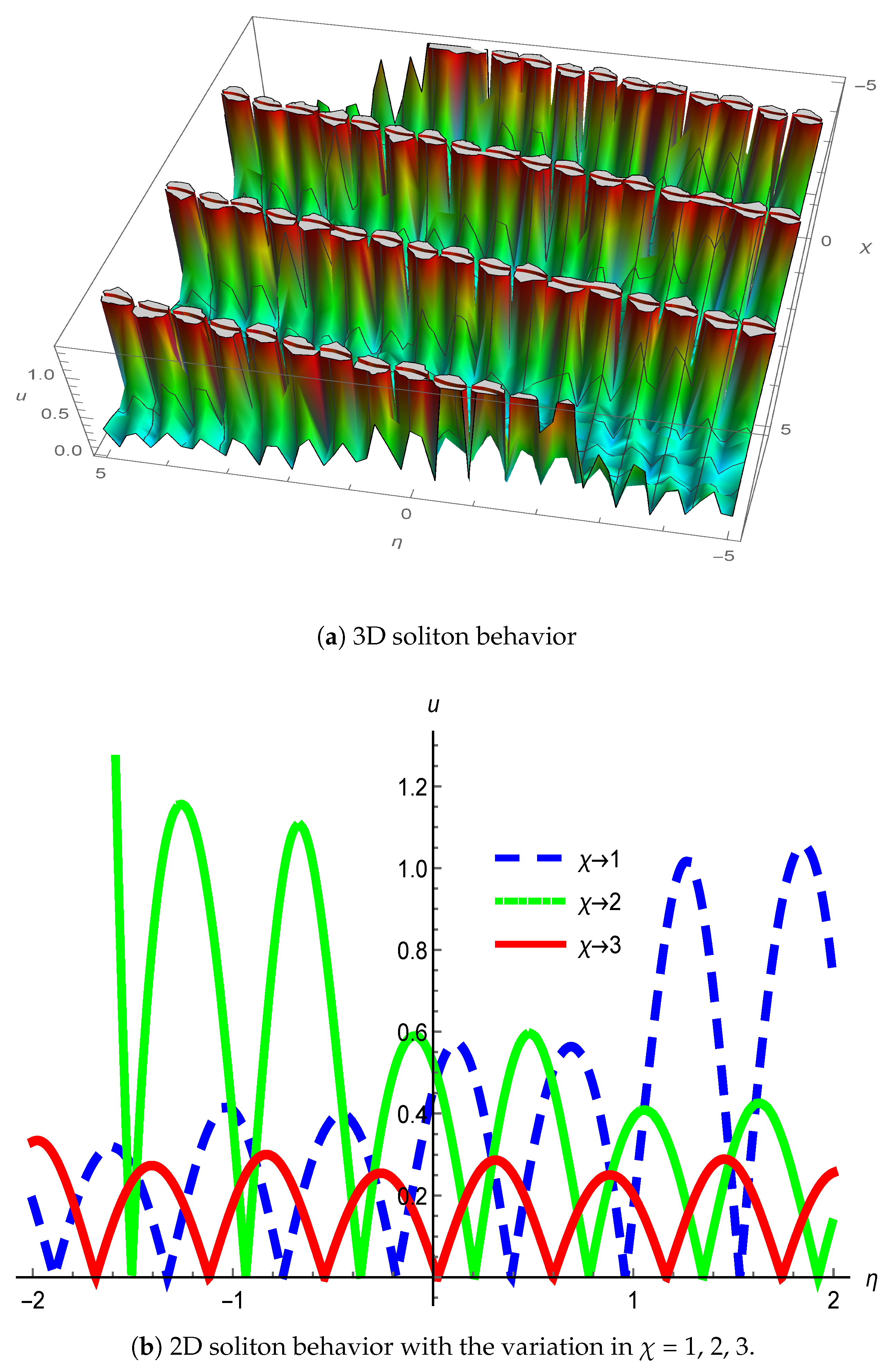
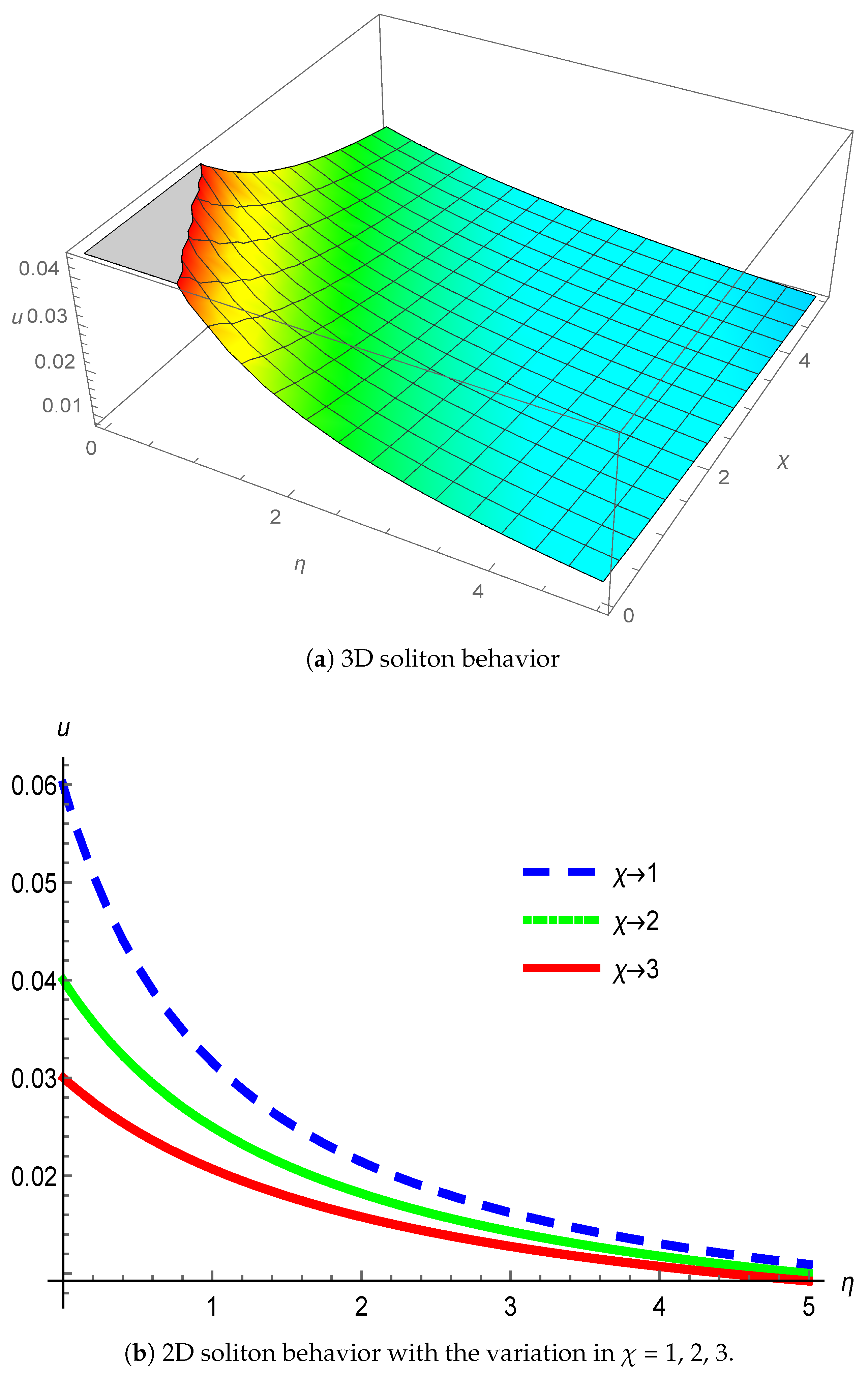
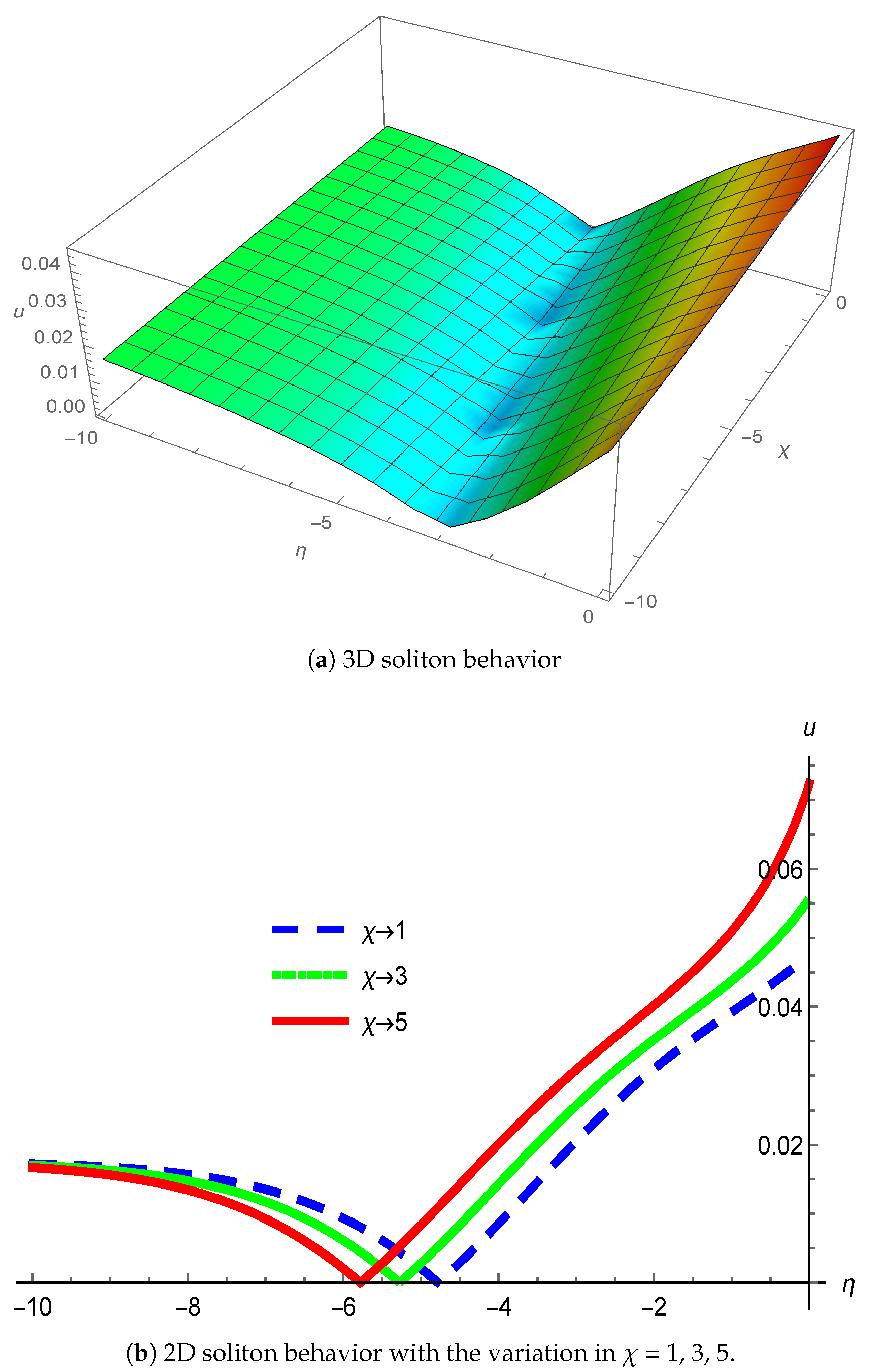
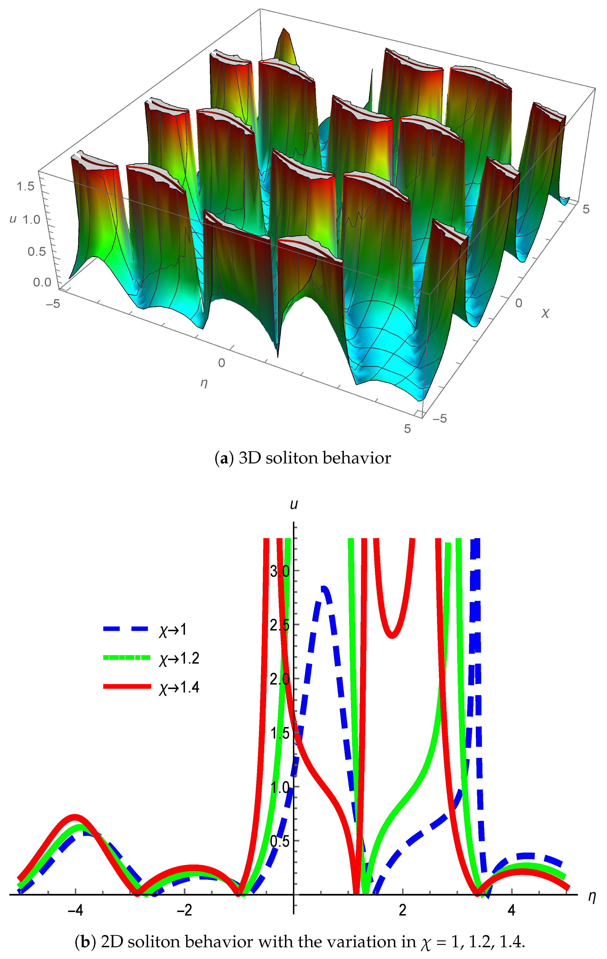
3. Physical Interpretation

The Whitham–Broer–Kaup (WBK), Boussinesq, and Kupershmidt equations are fundamental in studying wave propagation in non-linear and dispersive media, such as plasma. These equations capture the balance between non-linearity, which steepens waves, and dispersion, which spreads them over time. Analytical approaches reveal that a balance between strong non-local dispersion and quadratic non-linearity generates soliton—stable, localized wave packets. In plasma waves, different parametric values significantly affect solitonic behavior. Increased non-linearity results in solitons with larger amplitudes and higher frequencies, sustaining propagation over longer timescales. Conversely, increased dispersion produces wider and slower solitons. Analytical methods are ideal for investigating soliton characteristics, interactions, stability, and origins, while dynamics and stability of plasma waves can be specifically examined.

Figure 1 and Figure 2 illustrate the graphs of two Belyayev–Dykman waves, ${\mathsf{\Phi }}_1\left(\xi \right)$ and ${\mathsf{\Phi }}_4\left(\xi \right)$, highlighting how varying parametric values influence plasma wave behavior. Parameters $c_1=0.4,c_2=1.2,\rho =1.5,m=2,\kappa =0.1,\sigma =1.1$ affect the coefficients associated with non-linearity, dispersion, and external forces. Understanding how these parameters influence wave dynamics is crucial for predicting wave behavior in practical applications. The linear increment of wave amplitude is often presented through pedestal terms ${\mathsf{\Phi }}_1\left(\xi \right)$ and ${\mathsf{\Phi }}_4\left(\xi \right)$, leading to more intensive waves.

Solutions for ${\mathsf{\Phi }}_3\left(\xi \right)$ and ${\mathsf{\Phi }}_5\left(\xi \right)$ represent solitons with a kink-type wave for specific parameter values $c_1=0.1,c_2=0.2,\rho =1,m=1.2,\kappa =0.1$, and $\sigma =0.1$, as shown in Figure 3 and Figure 4. Smaller values of $\sigma =0.1$ illustrate the contour of kink waves. Wave speed is directly influenced by parameters that modify the medium’s properties or the wave’s interaction with the medium. Decreasing these parameters can slow down the wave, beneficial for situations requiring better stability or measurement accuracy.

Solutions for ${\mathsf{\Phi }}_8\left(\xi \right)$ represent solitons with a kink-type wave for parameter values $c_1=0.61,c_2=1.2,\rho =1.3,m=1.2,\kappa =0.4$, and $\sigma =2.1$ as shown in Figure 5. These parameters can lead to smoother, more predictable wave behavior. Understanding these interactions is essential in advanced plasma research and applications, where precise control over wave dynamics is necessary for achieving desired outcomes.

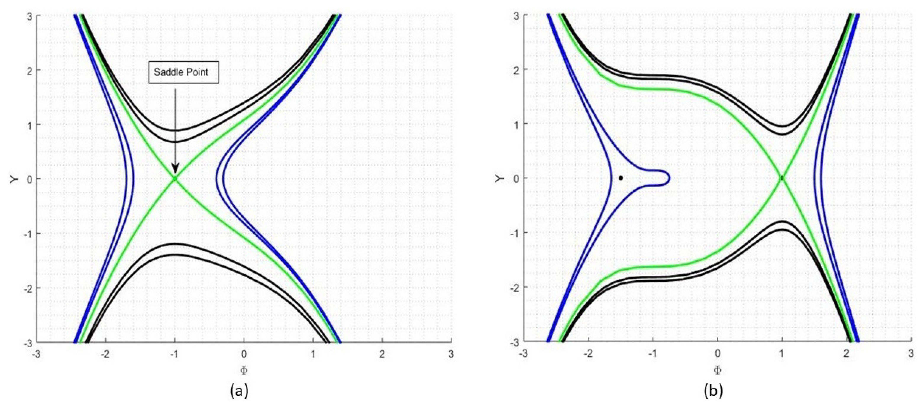
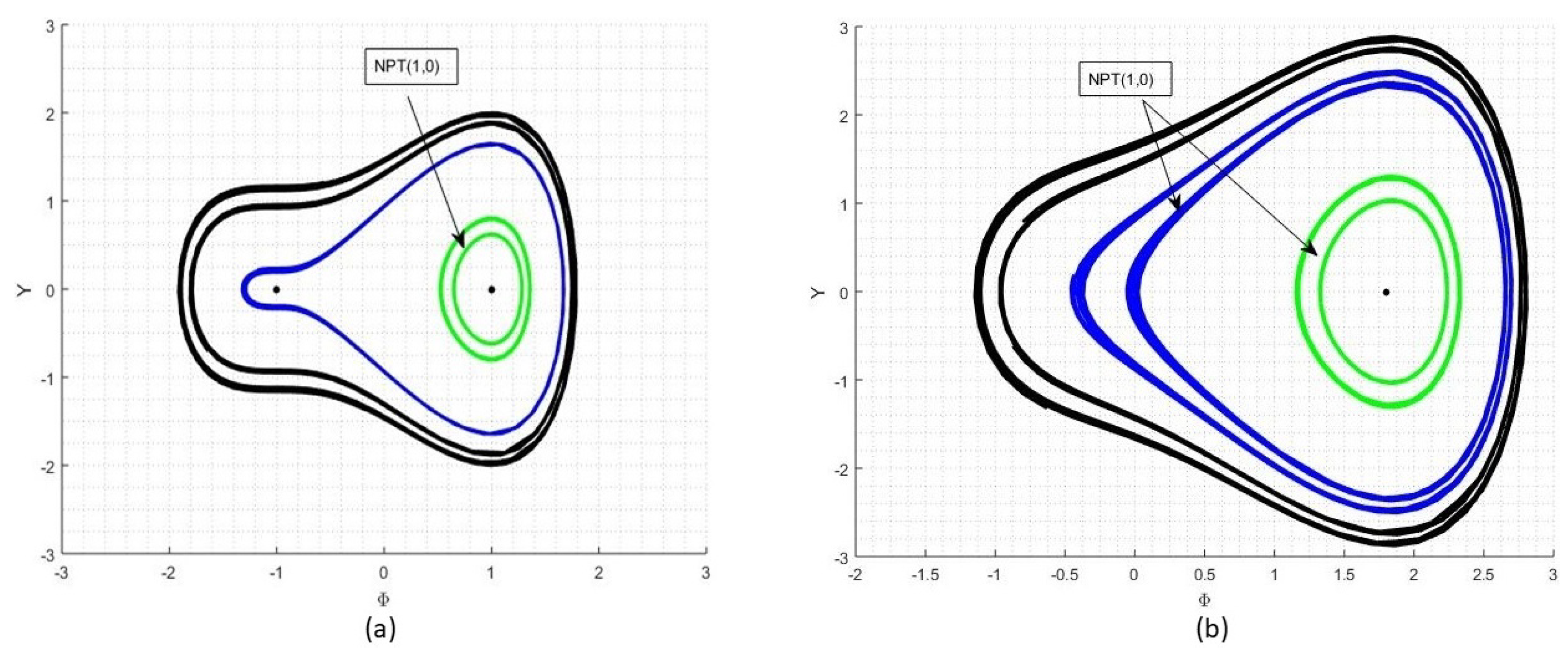
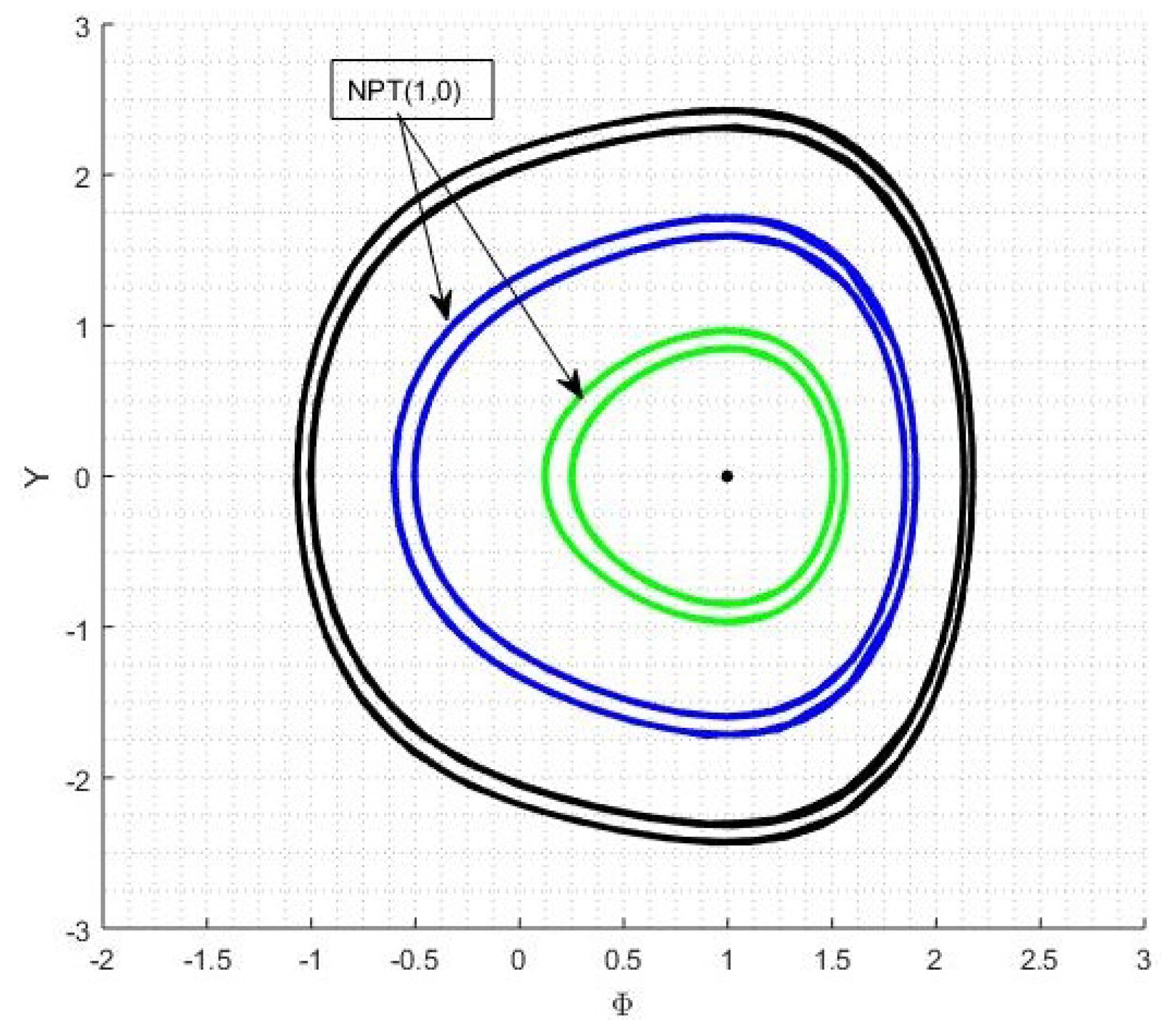
4. Bifurcation Theory

Equation (1) is analyzed through the lens of bifurcation. The study modifies the Galilean transformation Equation (8), assuming $C=0$:

$$\left\{\begin{array}{c}{\displaystyle \frac{d\mathsf{\Phi }}{d\xi }}=Y\hfill \\ {\displaystyle \frac{dY}{d\xi }}=A_1{\mathsf{\Phi }}^3+A_2{\mathsf{\Phi }}^2+A_3\mathsf{\Phi }\hfill \end{array}\right.$$

(27)

where $A_1={\displaystyle \frac{{\kappa }^2}{2(m^2+\rho \kappa )}}$, $A_2={\displaystyle \frac{3\sigma \kappa }{2(m^2+\rho \kappa )}}$, and $A_3={\displaystyle \frac{{\sigma }^2}{2(m^2+\rho \kappa )}}$. The equilibrium points of the system are ${\mathsf{\Phi }}_1=(0,0)$, ${\mathsf{\Phi }}_2=(E_1,0)$, and ${\mathsf{\Phi }}_3=(E_2,0)$, where $E_1$ and $E_2$ are defined as:

$$E_1={\displaystyle \frac{-A_2+\sqrt{A_2^2-4A_1{A}_3}}{2A_1}},\mathrm{and}{E}_2={\displaystyle \frac{-A_2-\sqrt{A_2^2-4A_1{A}_3}}{2A_1}}.$$

The planar dynamical structure concept is used to compute the equilibrium factor (${\mathsf{\Phi }}_i,Y_i$). A saddle point occurs when $J^{*}<0$, a zero point when $J^{*}=0$, and the Hopf index of (${\mathsf{\Phi }}_i,Y_i$) is zero, a node when $J^{*}>0$ and ${\tau }_1^2-4J^{*}>0$. In section (27), $J^{*}$ represents the Jacobian and ${\tau }_1$ the track coefficient matrix (M). Various trajectories in phase portraits, such as non-linear periodic trajectories (NPT) and non-linear homoclinic trajectories (NHT), are defined using the qualitative concept of dynamical structure. The phase diagrams represent equilibrium points (x) and separation layers (y), with assumed parameters $A_1=1$, $A_2=3$, and $A_3=1.4$.

4.1. Case 1

• $A_1>0$, $A_2>0$, $A_3>0$
• $A_1>0$, $A_2<0$, $A_3>0$

Figure 6a shows the phase portrait for given parameters $A_1$, $A_2$, and $A_3$. At the center ${\mathsf{\Phi }}_3=(-1,0)$, there is a single saddle point for open trajectories, implying that the plasma wave of Equation (8) survives in infinite open bounded trajectories. The phase portrait for $A_1$, $A_2$, and $A_3$ is shown in Figure 6b. At the center ${\mathsf{\Phi }}_2=(1,0)$, there is a single saddle point for open trajectories, implying that the plasma wave of Equation (8) survives in infinite open bounded trajectories.

4.2. Case 2

• $A_1>0$, $A_2>0$, $A_3<0$
• $A_1<0$, $A_2>0$, $A_3<0$
• $A_1<0$, $A_2<0$, $A_3<0$

Figure 7b shows the phase portrait for parameters $A_1$, $A_2$, and $A_3$. There is a single non-linear periodic trajectory at ${\mathsf{\Phi }}_3=(2,0)$, denoted by $NPT(1,0)$. The system (27) is represented by the infinite plasma wave of Equation (8). Figure 8 shows the phase portrait for parameters $A_1$, $A_2$, and $A_3$. There is a single non-linear periodic trajectory at ${\mathsf{\Phi }}_3=(1,0)$, denoted by $NPT(1,0)$. The system (27) is represented by the infinite plasma wave of Equation (8).

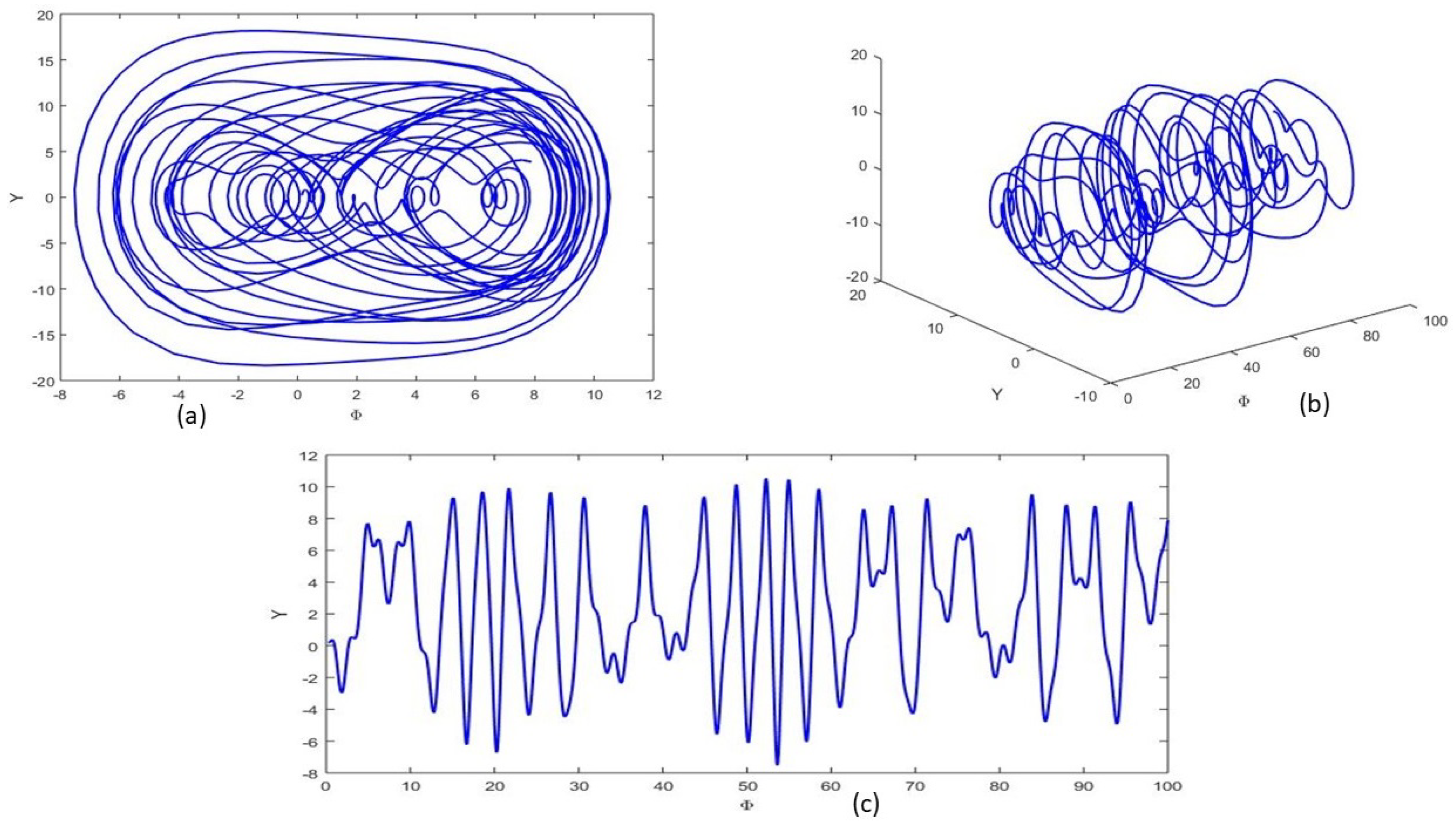
4.3. Chaotic Behavior

This section examines the discovered chaotic system. We supplement Equation (1) with the perturbation term $g_{0}cos\left(\omega \eta \right)$ to further excite the system. Changes to the dispersion properties and bifurcation dynamics of the equation may also affect the stability of solutions and the onset of chaotic behavior, as illustrated in Figure 9a–c. Depending on its specific qualities and form, the additional term may cause the system to enter chaotic dynamics. Using Equation (8), the following frame can be represented with an additional perturbation term:

$$\left\{\begin{array}{c}{\displaystyle \frac{d\mathsf{\Phi }}{d\xi }}=Y\hfill \\ {\displaystyle \frac{dY}{d\xi }}=A_1{\mathsf{\Phi }}^3+A_2{\mathsf{\Phi }}^2+A_3\mathsf{\Phi }+g_{0}cos\left(\omega \eta \right)\hfill \end{array}\right.$$

(28)

The parameters $A_1$, $A_2$, $A_3$, and $g_0$ are commonly used to indicate the amplitude of underlying forces or interactions in a chaotic system. Variations in $A_1$ can affect the overall dynamics of the system, influencing the formation, interaction, and propagation of plasma waves. Changes in $A_2$ and $A_3$ could affect the stability and structure of solutions to the WBK-BK equation, thereby impacting plasma wave behavior. For example, changes in $A_2$ may alter the plasma wave propagation frequency spectrum and impact processes like shock wave generation and wave packet dispersion. The addition of parameter $g_0$ in the bifurcation term can introduce spatial periodicity into the bifurcation dynamics, significantly impacting plasma wave behavior.

5. Sensitive Behavior

We examine the solution’s sensitive behavior in the system using the current dynamical framework (27). Figure 10a,b illustrates how initial conditions impact sensitively chaotic systems. Small changes in the initial state over time can cause trajectories to diverge significantly. Early disruptions in plasma waves have a significant effect on the system’s subsequent evolution, determining its trajectory and the object around which it converges.

6. Multi-Stable Chaotic System

We assess the multi-stability of the system (28) by examining the phase portrait and time series graph of the plasma wave with parametric values $\omega =1.29,A_1=-0.39,A_2=0.066,A_3=2.5$, and $g_0=-1.7$. The multi-stability chaotic systems depicted in Figure 11 display time series data along with a sensitive dependence on initial conditions. Small changes in initial conditions lead to different pathways, impacting resonance effects, dynamical modes, and stability of attractors. Plasma waves interacting with such a system can produce self-organized patterns and coherent structures.

7. Real-World Case Study: Chaos in Mode-Locked Fiber Lasers

Mode-locked fiber lasers are critical in generating ultra-short pulses of light for applications in high-speed optical communication, medical imaging, and precision measurements. These lasers rely on a delicate balance of dispersion and non-linearity within the fiber to produce and stabilize these pulses [22]. The insights from our investigation into non-linear plasma wave dynamics and chaos theory can be directly applied to mode-locked fiber lasers. By understanding the conditions under which these systems transition from stable mode-locking to chaotic pulse generation, engineers can proactively adjust system parameters such as pump power, fiber length, and dispersion management to maintain stability. Additionally, developing real-time feedback and control mechanisms can mitigate the effects of non-linearities, ensuring consistent and reliable pulse characteristics. This approach not only enhances pulse stability and reduces timing jitter but also improves overall system reliability and efficiency, demonstrating the practical application of our findings in optimizing the performance of mode-locked fiber lasers.

8. Conclusions

In this study, we investigate the dynamics of plasma waves using the generalized WBK-BK equations. We consider linear and non-linear perturbed and unperturbed cases. Through advanced mathematical methods, including the ${\displaystyle \frac{G^{\prime }}{G^2}}$ method, we derive new exact solutions revealing a wide range of complex behaviors in the systems. These methods provide a framework for predicting and analyzing the turbulence of plasma waves. We provide the circumstances under which the regular to chaotic states of the WBK-BK equations change, contributing to our understanding of chaos in non-linear systems. Our results highlight the powerful effects of tiny perturbations and linearity changes on the chaos and stability of non-linear waves. The conclusions drawn from our data processing methods and chaos analysis offer potential solutions for predicting and controlling chaotic behavior in plasma wave systems. This understanding is crucial for designing and managing systems where plasma waves play a dominant role. Our approach to fill the gap between plasma wave dynamics and general non-linear dynamic systems in physics and engineering, providing a tool for solving diverse problems encountered in these fields.

References

1. Kaufman, A.; Cohen, B. Theoretical plasma physics. J. Plasma Phys. 2019, 85, 205850601. [Google Scholar] [CrossRef]
2. Thomas, E.; Eadon, A.; Wallace, E. Suppression of low frequency plasma instabilities in a magnetized plasma column. Phys. Plasmas 2005, 12, 042109. [Google Scholar] [CrossRef]
3. Oloniiju, S.D. New sets of soliton solutions for the generalized Whitham–Broer–Kaup–Boussinesq–Kupershmidt system. Results Phys. 2023, 52, 106785. [Google Scholar] [CrossRef]
4. Jhangeer, A.; Muddassar, M.; Ur Rehman, Z.; Awrejcewicz, J.; Riaz, M.B. Multistability and dynamic behavior of non-linear wave solutions for analytical kink periodic and quasi-periodic wave structures in plasma physics. Results Phys. 2021, 29, 104735. [Google Scholar] [CrossRef]
5. Riaz, M.B.; Atangana, A.; Jhangeer, A.; Junaid-U-Rehman, M. Some exact explicit solutions and conservation laws of Chaffee-Infante equation by Lie symmetry analysis. Phys. Scr. 2021, 96, 084008. [Google Scholar] [CrossRef]
6. Houwe, A.; Sabi’u, J.; Hammouch, Z.; Doka, S.Y. Solitary pulses of a conformable nonlinear differential equation governing wave propagation in low-pass electrical transmission line. Phys. Scr. 2020, 95, 045203. [Google Scholar] [CrossRef]
7. Wazwaz, A.M. Exact Soliton and Kink Solutions for New (3 + 1)-Dimensional Nonlinear Modified Equations of Wave Propagation. Open Eng. 2017, 7, 169–174. [Google Scholar] [CrossRef]
8. Adeyemo, O.D. Applications of cnoidal and snoidal wave solutions via optimal system of subalgebras for a generalized extended (2 + 1)-D quantum Zakharov-Kuznetsov equation with power-law nonlinearity in oceanography and ocean engineering. J. Ocean. Eng. Sci. 2024, 9, 126–153. [Google Scholar] [CrossRef]
9. Samina, S.; Jhangeer, A.; Chen, Z. Bifurcation, chaotic and multistability analysis of the (2+1)-dimensional elliptic nonlinear Schrödinger equation with external perturbation. Waves Random Complex Media 2022, 15, 1–25. [Google Scholar] [CrossRef]
10. Shukla, P.K.; Mamun, A.A. Introduction to Dusty Plasma Physics. Plasma Phys. Control. Fusion 2002, 44, 395. [Google Scholar] [CrossRef]
11. Gu, C. Soliton Theory and Its Applications; Springer Science & Business Media: New York, NY, USA, 2013. [Google Scholar]
12. Ramamoorthy, R.; Rajagopal, K.; Leutcho, G.D.; Krejcar, O.; Namazi, H.; Hussain, I. Multistable dynamics and control of a new 4D memristive chaotic Sprott B system. Chaos Solitons Fractals 2022, 156, 111834. [Google Scholar] [CrossRef]
13. Lai, Q.; Akgul, A.; Li, C.; Xu, G.; Cavusoglu, U. A New Chaotic System with Multiple Attractors: Dynamic Analysis, Circuit Realization and S-Box Design. Entropy 2018, 20, 12. [Google Scholar] [CrossRef] [PubMed]
14. Rehman, Z.U.; Hussain, Z.; Li, Z.; Abbas, T.; Tlili, I. Bifurcation analysis and multi-stability of chirped form optical solitons with phase portrait. Results Eng. 2024, 21, 101861. [Google Scholar] [CrossRef]
15. Richardson, M.; Paxton, A.; Kuznetsov, N. Nonlinear methods for understanding complex dynamical phenomena in psychological science. APA Psychol. Sci. Agenda 2017, 31, 1–9. [Google Scholar]
16. Bains, A.S.; Misra, A.P.; Saini, N.S.; Gill, T.S. Modulational instability of ion-acoustic wave envelopes in magnetized quantum electron-positron-ion plasmas. Phys. Plasmas 2010, 17, 012103. [Google Scholar] [CrossRef]
17. Aljahdaly, N.H. Some applications of the modified (G’/G2)-expansion method in mathematical physics. Results Phys. 2019, 13, 102272. [Google Scholar] [CrossRef]
18. Guo, Y.; Yao, Z.; Xu, Y.; Ma, J. Control the stability in chaotic circuit coupled by memristor in different branch circuits. AEU-Int. J. Electron. Commun. 2022, 145, 154074. [Google Scholar] [CrossRef]
19. Al-Harbi, N.; Basfer, N.; Youssef, A.A.A. Exact solution of arrhenius equation under the square root heating model. Alex. Eng. J. 2023, 65, 475–479. [Google Scholar] [CrossRef]
20. Ghosh, U.N.; Chatterjee, P.; Roychoudhury, R. The effect of q-distributed electrons on the head-on collision of ion acoustic solitary waves. Phys. Plasmas 2012, 19, 012113. [Google Scholar] [CrossRef]
21. Nadeem, S.; Akhtar, S.; Alharbi, F.M.; Saleem, S.; Issakhov, A. Analysis of heat and mass transfer on the peristaltic flow in a duct with sinusoidal walls: Exact solutions of coupled PDEs. Alex. Eng. J. 2022, 61, 4107–4117. [Google Scholar] [CrossRef]
22. Bhowmike, N.; Rehman, Z.U.; Naz, Z.; Zahid, M.; Shoaib, S.; Amin, Y. Non-linear electromagnetic wave dynamics: Investigating periodic and quasi-periodic behavior in complex engineering systems. Chaos Solitons Fractals 2024, 184, 114984. [Google Scholar] [CrossRef]
Figure 1. In the WBK framework, Φ 1 ( ξ ) is graphed in 3D and 2D for the plasma wave, showing the wave’s amplitude in relation to its position.
Mathematics 12 02958 g001
Figure 2. In the WBK framework, Φ 4 ( ξ ) is graphed in 3D and 2D for the plasma wave, showing the relationship between wave amplitude and spatial position.
Mathematics 12 02958 g002
Figure 3. In the WBK framework, Φ 3 ( ξ ) is graphed in 3D and 2D for the plasma wave, showing the relationship between wave amplitude and spatial position.
Mathematics 12 02958 g003
Figure 4. In the WBK framework, Φ 5 ( ξ ) is graphed in 3D and 2D for the plasma wave, showing the relationship between wave amplitude and spatial position.
Mathematics 12 02958 g004
Figure 5. In the WBK framework, Φ 8 ( ξ ) is graphed in 3D and 2D for the plasma wave, showing the relationship between wave amplitude and spatial position.
Mathematics 12 02958 g005
Figure 6. Phase portraits for various unknown coefficient values. Case 1: for three conditions of A 1 , A 2 , and A 3 , the graph shows non-linear periodic behavior.
Mathematics 12 02958 g006
Figure 7. (a) Phase portraits for various unknown coefficient values. (b) Case 2: for three conditions of A 1 , A 2 , and A 3 , the graph shows super non-linear periodic behavior.
Mathematics 12 02958 g007
Figure 8. Phase portraits phenomena of dynamical system (27) for three conditions of A 1 , A 2 , and A 3 , which show periodic solution of the system.
Mathematics 12 02958 g008
Figure 9. Non-linear dynamical system for initial conditions ( 1.6 , 1.2 ) with parameters A 1 = 3.2 , A 2 = 1.4 , A 3 = 10.1 , and g 0 = 90 ,   ω = 1.5 .
Mathematics 12 02958 g009
Figure 10. Sensitive behavior of the system.
Mathematics 12 02958 g010
Figure 11. Multi-stability of the system.
Mathematics 12 02958 g011
Disclaimer/Publisher’s Note: The statements, opinions and data contained in all publications are solely those of the individual author(s) and contributor(s) and not of MDPI and/or the editor(s). MDPI and/or the editor(s) disclaim responsibility for any injury to people or property resulting from any ideas, methods, instructions or products referred to in the content.