Stochastic Phase Model with Reflective Boundary and Induced Beating: An Approach for Cardiac Muscle Cells

Abstract

We examine stochastic phase models for the community effect of cardiac muscle cells. Our model extends the stochastic integrate-and-fire model by incorporating irreversibility after beating, induced beating, and refractoriness. We focus on investigating the expectation and variance in the synchronized beating interval. Specifically, for a single isolated cell, we obtain the closed-form expectation and variance in the beating interval, discovering that the coefficient of variation has an upper limit of $\sqrt{2/3}$. For two coupled cells, we derive the partial differential equations for the expected synchronized beating intervals and the distribution density of phases. Furthermore, we consider the conventional Kuramoto model for both two- and N-cell models. We establish a new analysis using stochastic calculus to obtain the coefficient of variation in the synchronized beating interval, thereby improving upon existing literature.

1. Introduction

A cardiac muscle cell (cardiomyocyte) possesses a distinguishing property among biological cells: it generates spontaneous pulsation. The heartbeat is a macroscopic phenomenon in which the pulsations of cardiac muscle cells are synchronized to a certain rate. Given that each cell maintains its own beating rhythm when isolated, there must exist a mechanism for synchronizing the pulsations of cardiac muscle cells. Extensive research has been devoted to understanding this mechanism, both experimentally and theoretically [1,2,3,4,5,6,7,8,9,10,11,12,13,14]. The contraction of a cardiac muscle cell is caused by complex electrophysiological processes, and detailed analyses require elaborate mathematical models composed of a large number of equations [15]. However, to understand the essence of synchronization, a small number of simultaneous ordinary differential equations of membrane currents and action potentials, such as the Hodgkin–Huxley equation [16] or its reduced forms, the FitzHugh–Nagumo (FN) equation [17,18], and the Van der Pol equation (cf. [19,20]), are sufficient to capture the key phenomena of the cell dynamics.

Cardiac muscle cells in a tissue are individual entities with identical genetic information. However, these differences between individual cells are ironed out when they form clusters or tissues, a phenomenon known as the ’community effect’ of cells or induced uniformity [21,22]. Beyond the individual information (for example, the dynamics of the membrane currents of individual cells), a comprehensive understanding of cardiomyocyte dynamics requires analysis of the epigenetic information or the community effect. Given the difficulty in controlling the conditions and qualities of cells, there are limitations in biological experiments designed to study the community effect. To overcome these problems, mathematical modeling emerges as one of the most powerful approaches. In this paper, we aim to understand the community effect of cardiomyocytes by proposing and studying mathematical models that incorporate the essential properties of the biological system and can reproduce the experimental results to some extent [21,22].

To investigate the community effect of cardiomyocytes, we modify the conventional Kuramoto model [23,24] by incorporating the concepts of irreversibility of beating, induced beating, and refractoriness to capture the essential properties of cardiomyocyte synchronization. Our model can be regarded as a modification of the stochastic phase model or the integrate-and-fire model [25,26], which has been widely used as a spiking neuron model [27,28,29,30]. We utilize phase models for two reasons. First, from biological experiments [21,22], only data on beating intervals are available. However, the Hodgkin–Huxley, FitzHugh–Nagumo, or Van der Pol equations [16,17,18,19,20] model the dynamics of membrane currents or ion concentration. Without adequate information on potential and ion concentration, it is challenging to determine the parameters of these equations appropriately. Moreover, applying these models to each cell in an N-cell network ($N\gg 1$) yields a large number of nonlinear equations, which are difficult to handle. Next, since we mainly focus on investigating the beating intervals, one can consider a cardiomyocyte with rhythmic beating as an oscillator. Then, the phase models [23,24,31] are suitable mathematical tools to analyze the oscillation. In fact, the stochastic phase model is well-suited to model the distribution of the beating intervals (oscillation periods). For instance, in the case of a single isolated cell (single oscillator), one can determine the intrinsic frequency and noise strength of the phase model by the experimental data of beating intervals and the Formulas (10) and (12). In addition, one can derive the phase equation from the FN model (see [24]).

The main contributions of this paper can be summarized in two aspects. First, we introduce an original idea to incorporate the stochastic phase equation with a reflective boundary, induced pulsation, and refractoriness, to model the (synchronized) oscillation of cardiomyocytes. Hayashi et al. [32] compare the simulation of the proposed models with observations from biological experiments [21,22], which indicates the strong applicability of our models. This paper, serving as a theoretical supplement to [32], is devoted solely to theoretical analysis. For a single isolated cardiomyocyte, we obtain the explicit relationship between the model parameters (intrinsic frequency and noise strength) and the statistical properties (expectation and variance) of the beating interval. For two coupled cells, using renewal theory and the Fokker–Planck equation, we derive the partial differential equations (PDEs) associated with the expected synchronized beating intervals and the distribution density of phases. Although we cannot obtain the closed form of the statistical properties, the PDEs with nonstandard boundary conditions warrant comprehensive theoretical and numerical analysis from mathematical perspectives.

Secondly, we also consider the conventional phase model and make several improvements to the existing results [23]. Specifically, we present a rigorous calculation of the coefficient of variance (CV) for both two- and N-cell models using the theories of Itô integrals. Thanks to this, we provide formulas to determine the proper reaction coefficients of the model for the case of two-coupled cells.

The rest of this paper is organized as follows. In Section 2, we introduce the biological background of our work and explain the connection between the FitzHugh–Nagumo (FN) model and the phase equation. Section 3 is devoted to the model with a reflective boundary for a single isolated cell. We study the stochastic phase models for two-coupled cells in Section 4. The N-cell network is dealt with in Section 5. Concluding remarks are addressed in Section 6.

2. From the FitzHugh–Nagumo Model to the Phase Model

As a preliminary, we briefly introduce the experimental approach to understanding the epigenetic information of cardiomyocytes. And then, we explain the connection between the FN model and the phase model.

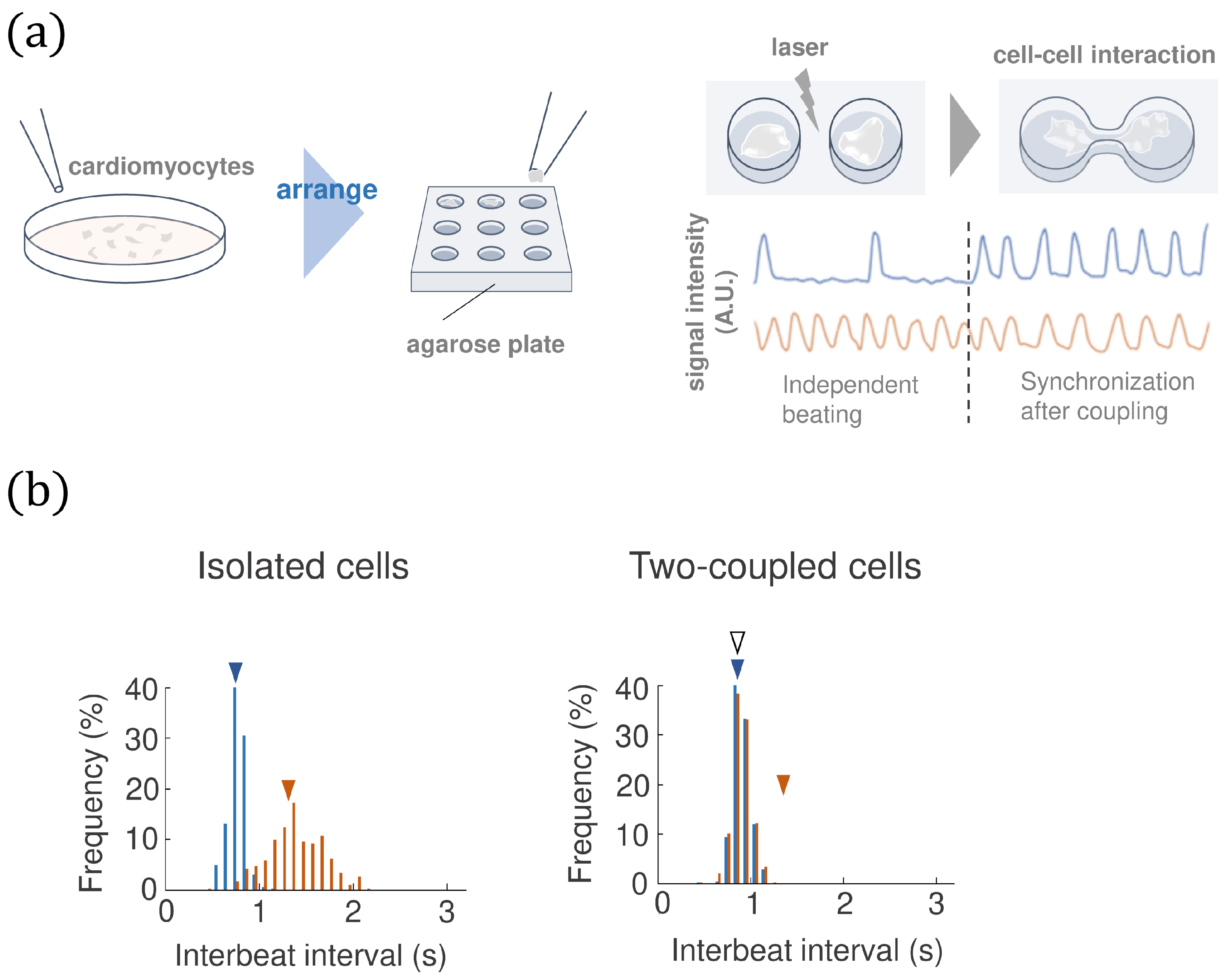
2.1. The Experimental Approach

The on-chip cellomics technology has been applied to investigating the community effect of cardiomyocytes [21,22], which, simply speaking, includes three steps: (1) The cells are taken from a community/tissue using a nondestructive cell sorting procedure. (2) We put the cells in a microchamber (on chip) where we can design the cell network and control the medium environment. (3) We measure the beating intervals of each cell on the chip by light signal (not the membrane currents). The procedure of the bio-experiment is described in Figure 1a (see [21,22] for details).

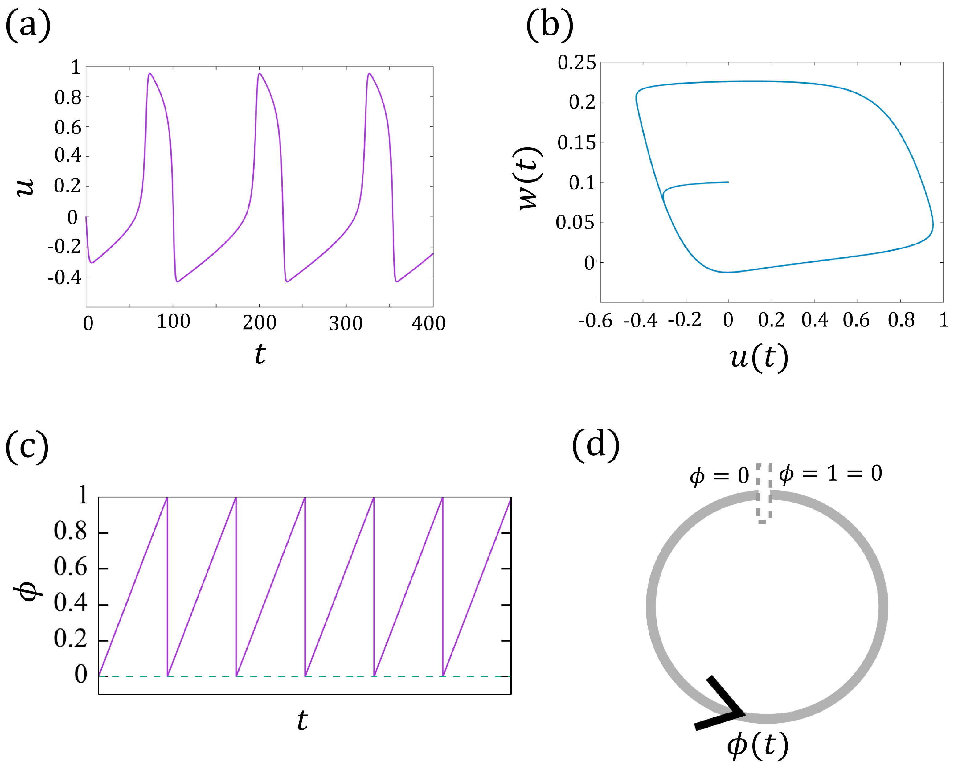
2.2. From the FitzHugh–Nagumo Model to the Phase Model

The FN model has been widely applied to model the membrane current of the spiking neuron or cardiomyocyte, which can be regarded as a simplification of the famous Hodgkin–Huxley model. First, let us pay attention to the case of the single cell without noise effect, the FN model of which is given by

$$\begin{array}{cc}\hfill & {\displaystyle \frac{du}{dt}}=u(u-a)(1-u)-w,\hfill \end{array}$$

(1a)

$$\begin{array}{cc}\hfill & {\displaystyle \frac{dw}{dt}}=\tau (u-bw).\hfill \end{array}$$

(1b)

Here, u denotes the membrane current, and $(a,b,\tau )$ the parameters ($\tau \ll 1$). When w decreases below 0, u increases instantly, which corresponds to the pulsation of the membrane potential (beating). Therefore, one can regard w as associated with the refractory (w also depends on u). For $a=-0.1$, $b=0.5$, $\tau =0.01$, we see that u behaves like a T-periodic function (see Figure 2a with $T\approx 108$). One can validate that, for sufficiently large time t, the trajectory $(u,w)$ tends to a limit cycle, that is, $\left(u\right(t+T),w(t+T\left)\right)=\left(u\right(t),w(t\left)\right)$ (see Figure 2b). Hence, one can find a homeomorphism that maps the points $\left(u\right(t),w(t\left)\right)$ on the limit cycle to the phase function $\varphi \left(t\right)$ given by

$$d\varphi \left(t\right)=\mu dt,$$

(2)

where $\mu ={\displaystyle \frac{1}{T}}$ denotes the intrinsic frequency (see [24] for the detailed argument). Here, $\varphi$ is also T-periodic if we set $\varphi =\varphi +k(\forall k\in \mathbb{Z})$, or equivalently, $\varphi$ takes value in torus $[0,1)$ (see Figure 2d), which means $\varphi$ jumps to 0 when approaching 1 ($\varphi \left(t\right)=0$ when $\varphi (t-):={lim}_{s\uparrow t}\varphi \left(s\right)=1$). See Figure 2c for an example of $\varphi$.

In brief, to model the dynamics of the membrane currents, one can apply the FN model involving two variables $(u,w)$ and parameters $(a,b,\tau )$. Meanwhile, to describe the rhythmic oscillation, the phase model with intrinsic frequency $\mu$ (or the beating interval T) is sufficient.

For two-coupled cells, let $u_1$ and $u_2$ represent the membrane currents for two cells, respectively, which satisfies the coupled FN model:

$$\begin{array}{cc}\hfill & {\displaystyle \frac{d{u}_1}{dt}}=u_1(u_1-a)(1-u_1)-w_1+\kappa (u_2-u_1),{\displaystyle \frac{d{w}_1}{dt}}=\tau (u_1-b{w}_1),\hfill \end{array}$$

(3a)

$$\begin{array}{cc}\hfill & {\displaystyle \frac{d{u}_2}{dt}}=u_2(u_2-a)(1-u_2)-w_2+\kappa (u_1-u_2),{\displaystyle \frac{d{w}_2}{dt}}=\tau (u_2-b{w}_2).\hfill \end{array}$$

(3b)

Here, $\kappa (u_i-u_j)$ describes the interaction between two cells. In Figure 3a,b, we show an example of the synchronization of $(u_1,u_2)$, where the trajectories $(u_1,w_1)$ and $(u_2,w_2)$ tend to the same limit cycle for sufficiently large time t.

If we adopt the Kuramoto model as the basic framework to study the synchronization behavior of two-coupled oscillators, the phase equations take the following form:

$$\begin{array}{cc}\hfill & {\displaystyle \frac{d{\varphi }_1}{dt}}=\mu +sin\left(2\pi ({\varphi }_1\left(t\right)-{\varphi }_2\left(t\right))\right),\hfill \\ \hfill & {\displaystyle \frac{d{\varphi }_2}{dt}}=\mu +sin\left(2\pi ({\varphi }_2\left(t\right)-{\varphi }_1\left(t\right))\right).\hfill \end{array}$$

(4)

where ${\varphi }_1$ and ${\varphi }_2$ represent the phases of the two cells, and $\mu$ is the intrinsic frequency. For more rigorous mathematical arguments, one can refer to [24].

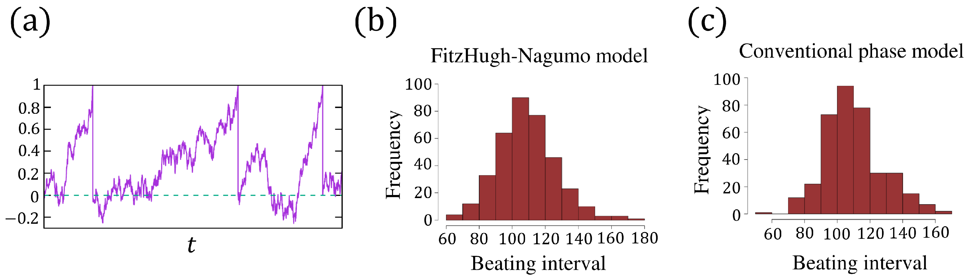
2.3. The FitzHugh–Nagumo and Phase Models with Noise

To analyze the distribution of the beating intervals from experiments (see Figure 1 (right)), one can apply the FN equations with noise to model the dynamics of the membrane currents. Figure 1b shows that the beating intervals of cardiomyocytes are not perfectly periodic, which indeed are affected by noise. Therefore, it is necessary to consider the FN model with noise:

$$\begin{array}{cc}\hfill & du=[u(u-a)(1-u)-w]dt+{\sigma }_{1}dW\left(t\right),\hfill \end{array}$$

(5a)

$$\begin{array}{cc}\hfill & dw=\tau (u-bw)dt,\hfill \end{array}$$

(5b)

where ${\sigma }_1>0$ denotes the noise strength, $dW\left(t\right)$ denotes the white noise, and $W\left(t\right)$ is the standard Brownian motion. A realization of the membrane current $u\left(t\right)$ and the trajectories $\left(u\right(t),w(t\left)\right)$ of (5a,b) is presented in Figure 3c,d.

Since the relationship between the distribution of beating interval and the parameters $(a,b,\tau ,{\sigma }_1)$ of the FN model has not been understood fully, the phase model with noise is applicable to study the beating process of cardiomyocytes, which is stated as follows:

$$\begin{array}{cc}\hfill & d\varphi \left(t\right)=\mu dt+\sigma dW\left(t\right),\hfill \end{array}$$

(6a)

$$\begin{array}{cc}\hfill & \varphi \left(0\right)=0,\hfill \end{array}$$

(6b)

where $\mu$ denotes the intrinsic frequency, and $\sigma >0$ the noise strength.

Define the beating interval $\Delta t:=t^{\left(k\right)}-t^{(k-1)}$ with $t^{\left(k\right)}$ the first passage time that $\varphi \left(t\right)=k$. Or, equivalently, we set $\varphi \left(t\right)=0$ when $\varphi (t-)=1$ (the phase jumps to 0 when reaching 1), and $\Delta t=t^{\left(k\right)}-t^{(k-1)}$ with $t^{\left(k\right)}:=inf\{t>t^{(k-1)}\mid \varphi (t-)=1\}$$(t^{\left(0\right)}=0)$. From (6a,b) and the definition of $\Delta t$, one can verify that

$$E(\Delta t)={\displaystyle \frac{1}{\mu }},Var(\Delta t)={\displaystyle \frac{{\sigma }^2}{{\mu }^3}},CV(\Delta t)=\sqrt{{\displaystyle \frac{Var(\Delta t)}{E{(\Delta t)}^2}}}={\displaystyle \frac{\sigma }{\sqrt{\mu }}}.$$

(7)

A sample path of $\varphi \left(t\right)$ in (6a,b) is shown in Figure 4a. We used the Euler–Maruyama method to solve this stochastic equation. The distribution of the beating intervals $\Delta t$ from Figure 3c is plotted in Figure 4b with a mean value $E(\Delta t)\approx 108.88$ and a standard variance $\sqrt{Var(\Delta t)}\approx 17.662$.

By (7), together with $E(\Delta t)=108.88$ and $\sqrt{Var(\Delta t)}=17.662$ (the simulation from FN model), we first compute the parameter $(\mu ,\sigma )=(0.0092,0.016)$, and then carry out the numerical simulation of (6a,b) and plot the distribution of the beating interval in Figure 4c. Although two distributions, Figure 4b,c, have the same mean value and variance, the density functions are not consistent with each other well. In view of the trajectory of $u\left(t\right)$ in Figure 3c, when $u\left(t\right)$ increases from $0.2$ to 1 and decreases from $0.6$ to $-0.1$ rapidly, the noise has little effect on the dynamic of u, as well as on the period of the oscillation cycle. In other words, when the action potential (the pulsation of u, or called beating) occurs, the noise effect is somehow inhibited such that the pulsation cannot be reversed by the noise. This irreversibility has not been captured by the phase model (6a,b), which may be the main reason causing the inconsistency between the distributions of Figure 4b,c. To address this issue, in the next section, we propose a phase model incorporating the irreversibility after beating.

3. The Phase Models for an Isolated Cell

The beating process in isolated cardiomyocytes is considered as the increase in a stochastic phase function from 0 to 1, where the phase starts at 0, increases with an intrinsic frequency $\mu$, and is affected by white noise with a strength of $\sigma$. When the phase approaches 1, the cell is said to beat, and the phase returns to 0. Thus, from 0 to 1, the cell completes one oscillation cycle. To account for the irreversibility of the beating process, we consider the stochastic phase model with a reflective boundary at the 0 state:

$$\begin{array}{cc}\hfill & d\varphi \left(t\right)=\mu dt+\sigma dW\left(t\right)+dL\left(t\right),\hfill \end{array}$$

(8a)

$$\begin{array}{cc}\hfill & \varphi \left(0\right)=0,\hfill \end{array}$$

(8b)

$$\begin{array}{cc}\hfill & \varphi \left(t\right)=0\mathrm{when}\varphi (t-)=1,\hfill \end{array}$$

(8c)

where $\varphi \left(t\right)$ denotes the phase of an isolated cardiomyocyte at time t, and $W\left(t\right)$ represents the standard Brownian motion. $dW\left(t\right)$ is the generalized derivative of W(t), which is known as Gaussian white noise. We introduce the concept of irreversibility following a beat. When the cell beats, we have $\varphi (t-)=1$ and $\sigma dW(t-)<0$; the phase may become negative, i.e., $\varphi \left(t\right)$ reverts to 1. The irreversibility dictates that when $\varphi (t-)=0$, $\varphi$ cannot be driven back to 1 by negative noise. To prevent the reversibility of beating, we add the process $L\left(t\right)$ to cancel the negative part of the noise, ensuring that $\varphi \left(t\right)\ge 0$ always holds. $L\left(t\right)$ effectively describes the reflective boundary at $\varphi =0$ (cf. [33,34,35]).

$$t^{\left(k\right)}=inf\{t>t^{(k-1)}:\varphi (t-)=1\},t^{\left(0\right)}=0.$$

(9)

We say the cell beats at $t^{\left(k\right)}$ ($k=1,2,\dots$). In view of (8c), when $\varphi$ approaches 1 (i.e., $\varphi (t^{\left(k\right)}-)=1$), $\varphi$ immediately jumps to 0, i.e., $\varphi \left(t^{\left(k\right)}\right)=0$, and a new oscillation cycle begins. The rigorous definition of $L\left(t\right)$ is given as follows (see Figure 5a):

(L1)

$L\left(0\right)=0$, and $L\left(t\right)$ is a nondecreasing, continuous process for $t^{(k-1)}\le t<t^{\left(k\right)}$ such that $\varphi \left(t\right)\ge 0$;

(L2)

$L\left(t\right)$ increases only when $\varphi \left(t\right)=0$.

In simulation, a simple approach [36] is to reset $\varphi \left(t_n\right)=0$ when $\varphi \left(t_n\right)=\varphi \left(t_{n-1}\right)+\mu \Delta t+\sqrt{\Delta t}\sigma \eta <0$, where $\Delta t$ denotes the time-step ($\Delta t\ll 1$), $t_n=n\Delta t$$(n=1,2,\cdots ,)$ and $\eta \sim \mathcal{N}(0,1)$.

During the first beating process, i.e., $t\in [0,t^{\left(1\right)})$, integrating (8a) yields

$$\varphi \left(t\right)=\underset{=:X\left(t\right)}{\underbrace{\mu t+\sigma W\left(t\right)}}+L\left(t\right),$$

which means $\varphi \left(t\right)$ is in fact a combination of the $(\mu ,\sigma )$-Brownian motion $X\left(t\right)$ and the process $L\left(t\right)$. We plot an example of $\left(\varphi \right(t),X(t),L(t\left)\right)$ for $t\in [0,t^{\left(1\right)})$ in Figure 5a. Since $\varphi$ returns to 0 instantly when approaching 1, $\varphi \left(t\right)$ is a renewal process for $t\ge t^{\left(k\right)}$ ($k=1,2,\cdots$) (see Figure 5b), and the beating intervals (oscillation period) $\Delta t^{\left(k\right)}:=t^{\left(k\right)}-t^{(k-1)}$ ($k=1,2,\dots$) are independent, identically distributed random variables. Hence, we only need to investigate $\Delta t^{\left(1\right)}=t^{\left(1\right)}-0$.

Theorem 1. 

For $\mu \ge 0$, $\sigma >0$, we have

$$E\left(t^{\left(1\right)}\right)=\left\{\begin{array}{ccc}\hfill & 1/{\sigma }^2\hfill & \hfill \mathrm{for}\mu =0,\\ \hfill & (\theta -1+e^{-\theta })/\left(\mu \theta \right)\hfill & \hfill \mathrm{for}\mu >0,\end{array}\right.$$

(10)

$$Var\left(t^{\left(1\right)}\right)=\left\{\begin{array}{ccc}\hfill & 2/\left(3{\sigma }^4\right)\hfill & \hfill \mathrm{for}\mu =0,\\ \hfill & e^{-\theta }(e^{-\theta }-5e^{\theta }+2\theta e^{\theta }+4+4\theta )/\left({\mu }^2{\theta }^2\right)\hfill & \hfill \mathrm{for}\mu >0,\end{array}\right.$$

(11)

where $\theta =2\mu /{\sigma }^2$.

See Appendix A for the proof of Theorem 1.

Corollary 1. 

Throughout this paper, we always consider the non-negative intrinsic frequency $(\mu \ge 0)$ and positive noise strength $(\sigma >0)$. Passing to the limit $\mu \to 0$, one can validate ${\displaystyle \frac{\theta -1+e^{-\theta }}{\mu \theta }}\to {\displaystyle \frac{1}{{\sigma }^2}}$ and ${\displaystyle \frac{e^{-\theta }(e^{-\theta }-5e^{\theta }+2\theta e^{\theta }+4+4\theta )}{{\mu }^2{\theta }^2}}\to {\displaystyle \frac{2}{3{\sigma }^4}}$. The coefficient of variance (CV) is given by:

$$C{V}^2\left(t^{\left(1\right)}\right)={\displaystyle \frac{Var(\Delta t)}{E^2(\Delta t)}}=\left\{\begin{array}{ccc}\hfill & 2/3\hfill & \hfill \mathrm{for}\mu =0,\\ \hfill & K\left(\theta \right)\hfill & \hfill \mathrm{for}\mu >0,\end{array}\right.$$

(12)

where $K\left(\theta \right)={\displaystyle \frac{e^{\theta }(e^{-\theta }-5e^{\theta }+2\theta e^{\theta }+4+4\theta )}{{(1+\theta e^{\theta }-e^{\theta })}^2}}$ and $K\left(\theta \right)\uparrow 2/3$ as $\theta \downarrow 0$.

Consequently, the current model (8a) is only applicable to cardiomyocytes with a CV of less than $\sqrt{2/3}$.

We are able to calculate the mean value and the CV of the beating interval using the experimental data. From (12), we initially determine $\theta$. Subsequently, with $\theta$ and the mean value, the coefficients $(\mu ,\sigma )$ can be computed using (10). The suitability of our model, as described in Equation (8a–c), for the bio-experimental data is discussed in the work of [32].

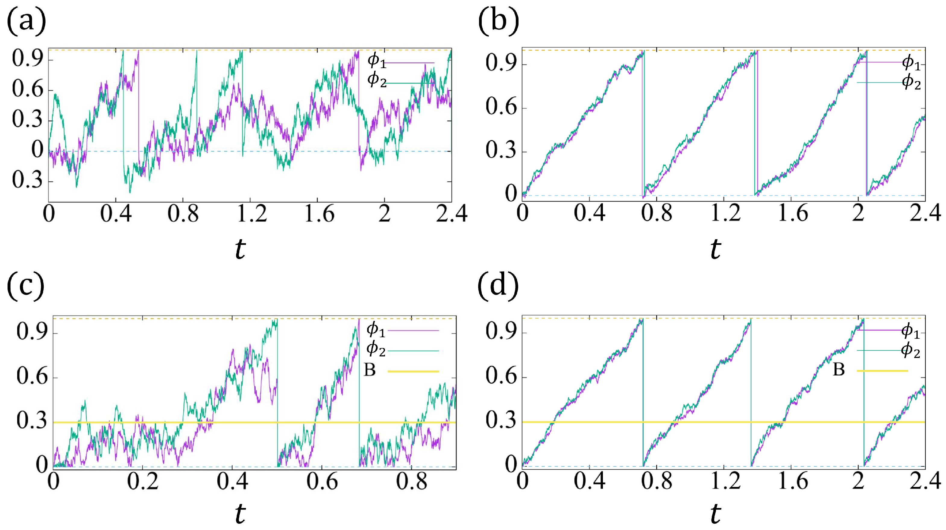
4. The Phase Models for Two Coupled Cells

As explained in Section 2, the Kuramoto model is an applicable tool to investigate the synchronization beating of two-coupled cardiomyocytes. The conventional Kuramoto model with noise effect for two-coupled oscillators ${\left\{{\overline{\varphi }}_i\right\}}_{i=1,2}$ is presented as follows:

$$\begin{array}{cc}\hfill & d{\overline{\varphi }}_i\left(t\right)={\mu }_{i}dt+A_{i,j}f({\overline{\varphi }}_j-{\overline{\varphi }}_i)dt+{\sigma }_{i}d{W}_i\left(t\right),\hfill \end{array}$$

(13a)

$$\begin{array}{cc}\hfill & {\overline{\varphi }}_i\left(0\right)=0,\hfill \end{array}$$

(13b)

where $i,j=1,2$, $i\ne j$, $f\left(x\right)=sin\left(2\pi x\right)$, $({\mu }_i,{\sigma }_i)$ denotes the intrinsic frequency and noise strength for cell (oscillator) i, $A_{i,j}$ the coefficient describing the strength of reaction between cell i and cell j ($A_{i,j}\ge 0$), and ${\left\{W_i\left(t\right)\right\}}_{i=1,2}$ the two independent standard Brownian motions.

However, in general cases, the above model may be inadequate to capture the essential properties of cardiomyocytes’ synchronization. First, the irreversibility of beating should be taken into account. Second, the cardiomyocyte can be induced to beat by the neighboring cells’ action potential. In addition, after beating, the cardiomyocyte enters a refractory period, during which the cell cannot be induced to beat. The length of the refractory period depends on the membrane potential, or more precisely, on the concentrations of Ca²⁺, K⁺, Na⁺ ions inside and outside the membrane.

To incorporate the irreversibility of beating, induced beating, and refractory, we modify the conventional Kuramoto model (4) as follows. Let ${\left\{{\varphi }_i\right\}}_{i=1,2}$ be the phase of two cardiomyocytes, satisfying

$$\begin{array}{cc}\hfill & d{\varphi }_i\left(t\right)={\mu }_{i}dt+A_{i,j}f({\varphi }_j-{\varphi }_i)dt+{\sigma }_{i}d{W}_i\left(t\right)+d{L}_i\left(t\right),\hfill \end{array}$$

(14a)

$$\begin{array}{cc}\hfill & {\varphi }_i\left(0\right)=0,\hfill \end{array}$$

(14b)

where the process $L_i\left(t\right)$ imposes the reflective boundary for ${\varphi }_i$. Let $t_i^{\left(k\right)}$ be the k-th passage time that cell i beats. Then, we call $[t_i^{\left(k\right)},t_i^{(k+1)})$ the k-th beating interval (or oscillation cycle) of cell i. $L_i$ is defined by:

(L1)

$L_i$ is continuous and nondecreasing during each beating interval of ${\varphi }_i$;

(L2)

$L_i$ increases only when ${\varphi }_i=0$.

Since the refractory period associates with the membrane potential (u of FN model), which corresponds to the phase ${\varphi }_i$, for simplicity, we set a refractory threshold $B_i$ ($0\le B_i<1$) and implement the induced beating and refractory by the following:

(IND)

If cell i is out of refractory, cell i beats promptly when the neighbor (cell j) beats spontaneously; in other words, if ${\varphi }_i(t-)>B_i$ and ${\varphi }_j(t-)=1$, then ${\varphi }_j\left(t\right)={\varphi }_i\left(t\right)=0$ (both two phases jump to 0 after beating to start a new oscillation cycle);

(REF)

If cell i is in refractory and the neighbor cell j beats spontaneously, then cell i will not be induced to beat, namely, if ${\varphi }_i(t-)\le B_i$ and ${\varphi }_j(t-)=1$, then ${\varphi }_j\left(t\right)=0$ and ${\varphi }_i\left(t\right)={\varphi }_i(t-)$ (${\varphi }_j$ jumps to 0 but ${\varphi }_i$ keeps going).

Remark 1. 

One weak point of the conventional model (13a,b) is that the synchronization has been treated as “ambiguous” or “approximately”, because the possibility of ${\overline{\varphi }}_i\left(t\right)={\overline{\varphi }}_j\left(t\right)=1$ is zero, and one can only expect that both two cells beat with tiny time-delay, namely, ${\overline{\varphi }}_i\left(t_i\right)=1$, ${\overline{\varphi }}_j\left(t_j\right)=1$ with $|t_i-t_j|\approx 0$. To guarantee this “approximated” synchronization, one should take sufficiently small noise strength ${\sigma }_i$ and large enough reaction coefficient $A_{i,j}$ (see Section 4.2).

Thanks to the induced beating (IND), we have a rigorous mathematical definition of the synchronization. Let ${\mathbf{t}}^{\left(k\right)}$ denote the time of k-th synchronized beating, i.e.,

$${\mathbf{t}}^{\left(k\right)}:=inf\{t>{\mathbf{t}}^{(k-1)}:{\varphi }_i(t-)=1,{\varphi }_j\left(t\right)>B_j,i=1\mathrm{or}2,j\ne i\}({\mathbf{t}}^{\left(0\right)}=0).$$

(15)

In view of ${\varphi }_1\left({\mathbf{t}}^{\left(k\right)}\right)={\varphi }_2\left({\mathbf{t}}^{\left(k\right)}\right)=0$, $\mathrm{\Phi }\left(t\right):=({\varphi }_1\left(t\right),{\varphi }_2\left(t\right))$ is a renewal stochastic process for $t>{\mathbf{t}}^{\left(k\right)}$$(k=0,1,2,\cdots )$. Therefore, the beating intervals ${\{{\mathbf{t}}^{(k+1)}-{\mathbf{t}}^{\left(k\right)}\}}_{k\ge 0}$ are independent and identically distributed (i.i.d.). To obtain the expected value and variance of synchronized beating interval, we only need to investigate ${\mathbf{t}}^{\left(1\right)}$.

In Figure 6, we plot two examples of $({\overline{\varphi }}_1,{\overline{\varphi }}_2)$ and $({\varphi }_1,{\varphi }_2)$, respectively. For small noise strength and large reaction coefficients, for example, ${\sigma }_1={\sigma }_2=0.2$, $A_{1,2}=A_{2,1}=6$, the conventional model (13a,b) (Figure 6b) and the proposed model (14a,b) have a similar solution behavior (Figure 6d). Considering Figure 6b, the nonpositive phase (${\overline{\varphi }}_i\le 0)$ can be ignored, and the time delay between two cells’ beating is very tiny. Therefore, the roles of the reflective boundary and induced beating in our model are negligible. However, when the noise strength is not so small and the reaction coefficients are not large enough, the conventional model $({\overline{\varphi }}_1,{\overline{\varphi }}_2)$ may not synchronize (see Figure 6a), whereas Figure 6c shows the synchronization owing to the induced beating and the significant role of the reflective boundary.

We intend to calculate the expected value and variance for the synchronized beating interval ${\mathbf{t}}^{\left(1\right)}$. First, for the proposed model, applying Ito’s calculus and the renewal theory, we derive the PDEs associated with $E\left({\mathbf{t}}^{\left(1\right)}\right)$ and $Var\left({\mathbf{t}}^{\left(1\right)}\right)$. However, the closed-form of the PDEs’ solutions is nontrivial to derive. Next, we consider the case that the role of the reflective boundary and induced beating is negligible, where the conventional and proposed models have little difference, and we obtain the relationship between the parameters and the CV of beating intervals.

4.1. The Expectation and Variance in the Synchronized Beating Interval

Besides the synchronized beating (induced beating (IND)), let us pay attention to the single-beating (REF), or called independent-beating, where only one cell is beating and the other is in refractory. Assume that before the first synchronized beating, cell i beats independently for $J_i$ times. Let $t_i^{\left(m\right)}$$(m\le J_i)$ be the passage time of the m-th single-beating of cell i, that is,

$$t_i^{\left(m\right)}:=inf\{t>t_i^{(m-1)}:{\varphi }_i(t-)=1,{\varphi }_j\left(t\right)<B_j,t<{\mathbf{t}}^{\left(1\right)}\},t_i^{\left(0\right)}=0(j\ne i).$$

(16)

For $t<{\mathbf{t}}^{\left(1\right)}$, ${\varphi }_i\left(t\right)$ is a stochastic process with a jump at ${\left\{t_i^{\left(m\right)}\right\}}_{m=1}^{J_i}$, where ${\varphi }_i(t_i^{\left(m\right)}-)=1$ and ${\varphi }_i\left(t_i^{\left(m\right)}\right)=0$. Setting $\mathrm{\Phi }\left(t\right):=({\varphi }_1\left(t\right),{\varphi }_2\left(t\right))$, and applying the Itô’s formula for the stochastic process with jumps (cf. [33]), we have, for any $g(x_1,x_2)$$(0\le x_1,x_2\le 1)$ with continuous differential ${\displaystyle \frac{\partial g}{\partial x_i}}$ and ${\displaystyle \frac{{\partial }^{2}g}{\partial x_i\partial x_j}}$ ($i,j=1,2$),

$$\begin{array}{cc}\hfill & g\left(\mathrm{\Phi }({\mathbf{t}}^{\left(1\right)}-)\right)=g\left(\mathrm{\Phi }\left(0\right)\right)+{\int }_0^{{\mathbf{t}}^{\left(1\right)}}\sum _{i=1}^2\left[({\mu }_i+A_{i,j}f(x_j-x_i)){\displaystyle \frac{\partial }{\partial x_i}}+{\displaystyle \frac{{\sigma }_i^2}{2}}{\displaystyle \frac{{\partial }^2}{\partial x_i^2}}\right]g\left(\mathrm{\Phi }\left(s\right)\right)ds\hfill \\ \hfill & +{\int }_0^{{\mathbf{t}}^{\left(1\right)}}\sum _{i=1}^2{\sigma }_i{\displaystyle \frac{\partial g}{\partial x_i}}\left(\mathrm{\Phi }\left(s\right)\right)d{W}_i\left(s\right)+\sum _{i=1}^2{\int }_0^{{\mathbf{t}}^{\left(1\right)}}{\displaystyle \frac{\partial g}{\partial x_i}}\left(\mathrm{\Phi }\left(s\right)\right)d{L}_i\left(s\right)\hfill \\ \hfill & -\sum _{m=1}^{J_1}\left[g(1,{\varphi }_2(t_1^{\left(m\right)}-))-g(0,{\varphi }_2\left(t_1^{\left(m\right)}\right))\right]-\sum _{m=1}^{J_2}\left[g({\varphi }_1(t_2^{\left(m\right)}-),1)-g({\varphi }_1\left(t_2^{\left(m\right)}\right),0)\right],\hfill \end{array}$$

(17)

where ${\varphi }_i\left(t_j^{\left(m\right)}\right)={\varphi }_i(t_j^{\left(m\right)}-)\le B_i$, that is, cell j is in refractory while cell i is beating (${\varphi }_i(t_i^{\left(m\right)}-)=1$). Since $L_i\left(t\right)$ is nondecreasing in the time intervals ${\left\{(t_i^{\left(m\right)},t_i^{(m+1)})\right\}}_{m=0}^{J_{i-1}}$ and $(t_i^{\left(J_i\right)},{\mathbf{t}}^{\left(1\right)})$, and $L_i\left(t\right)$ increases only when ${\varphi }_i\left(t\right)=0$, we see that

$${\int }_0^{{\mathbf{t}}^{\left(1\right)}}{\displaystyle \frac{\partial g}{\partial x_i}}\left(\mathrm{\Phi }\left(s\right)\right)d{L}_i\left(s\right)={\int }_{\{0<s<{\mathbf{t}}^{\left(1\right)}\mid {\varphi }_i\left(s\right)=0\}}{\displaystyle \frac{\partial g}{\partial x_i}}\left(\mathrm{\Phi }\left(s\right)\right)d{L}_i\left(s\right)$$

(18)

Let g be the solution of (19a–f):

$$\begin{array}{ccc}\hfill & \sum _{i=1}^2\left[({\mu }_i+A_{i,j}f(x_j-x_i)){\displaystyle \frac{\partial }{\partial x_i}}+{\displaystyle \frac{{\sigma }_i^2}{2}}{\displaystyle \frac{{\partial }^2}{\partial x_i^2}}\right]g=-1\hfill & \hfill \mathrm{for}0<x_1,x_2<1,\end{array}$$

(19a)

$$\begin{array}{cc}{\displaystyle \frac{\partial g}{\partial x_i}}=0\hfill & \hfill \mathrm{for}{x}_i=0,i=1,2,\end{array}$$

(19b)

$$\begin{array}{cc}g(1,x_2)=0\hfill & \hfill \mathrm{for}{B}_2<x_2\le 1,\end{array}$$

(19c)

$$\begin{array}{cc}g(x_1,1)=0\hfill & \hfill \mathrm{for}{B}_1<x_1\le 1,\end{array}$$

(19d)

$$\begin{array}{cc}g(x_1,0)=g_2(x_1,1)\hfill & \hfill \mathrm{for}0\le x_1\le B_1,\end{array}$$

(19e)

$$\begin{array}{cc}g(0,x_2)=g_2(1,x_2)\hfill & \hfill \mathrm{for}0\le x_2\le B_2.\end{array}$$

(19f)

It follows from (19b) and (18) that

$${\int }_0^{{\mathbf{t}}^{\left(1\right)}}{\displaystyle \frac{\partial g}{\partial x_i}}\left(\mathrm{\Phi }\left(s\right)\right)d{L}_i\left(s\right)=0.$$

Since the induced beating happens at $t={\mathbf{t}}^{\left(1\right)}$, we have ${\varphi }_1({\mathbf{t}}^{\left(1\right)}-)=1,{\varphi }_2({\mathbf{t}}^{\left(1\right)}-)>B_2$ or ${\varphi }_2({\mathbf{t}}^{\left(1\right)}-)=1,{\varphi }_1({\mathbf{t}}^{\left(1\right)}-)>B_1$, which, together with (19c) and (19d), implies

$$g\left(\mathrm{\Phi }({\mathbf{t}}^{\left(1\right)}-)\right)=0.$$

Furthermore, in view of ${\varphi }_i\left(t_j^{\left(m\right)}\right)={\varphi }_i(t_j^{\left(m\right)}-)\le B_i$, (19e) and (19f) guarantee that

$$\sum _{m=1}^{J_1}\left[g(1,{\varphi }_2(t_1^{\left(m\right)}-))-g(0,{\varphi }_2\left(t_1^{\left(m\right)}\right))\right]=0,\sum _{m=1}^{J_2}\left[g({\varphi }_1(t_2^{\left(m\right)}-),1)-g({\varphi }_1\left(t_2^{\left(m\right)}\right),0)\right]=0.$$

With $\mathrm{\Phi }\left(0\right)=(0,0)$ and (19a), we rewrite (17) into the following:

$$\begin{array}{c}\hfill 0=g(0,0)-{\mathbf{t}}^{\left(1\right)}+{\int }_0^{{\mathbf{t}}^{\left(1\right)}}\sum _{i=1}^2{\sigma }_i{\displaystyle \frac{\partial g}{\partial x_i}}\left(\mathrm{\Phi }\left(s\right)\right)d{W}_i\left(s\right)\end{array}$$

(20)

Taking the expectation, we have

$$E\left[{\mathbf{t}}^{\left(1\right)}\right]=g(0,0)+\underset{=0}{\underbrace{E\left[{\int }_0^{{\mathbf{t}}^{\left(1\right)}}{\sum }_{i=1}^2{\sigma }_i{\displaystyle \frac{\partial g}{\partial x_i}}\left(\mathrm{\Phi }\left(s\right)\right)d{W}_i\left(s\right)\right]}}=g(0,0).$$

(21)

Hence, the obtention of $E\left({\mathbf{t}}^{\left(1\right)}\right)$ reduces to solve the PDE (19a–f). Next, let us turn attention to the variance $Var\left[{\mathbf{t}}^{\left(1\right)}\right]$. From (20), we have

$$\begin{array}{cc}\hfill {\left({\mathbf{t}}^{\left(1\right)}\right)}^2={\left(g(0,0)\right)}^2+& {\left[{\int }_0^{{\mathbf{t}}^{\left(1\right)}}\sum _{i=1}^2{\sigma }_i{\displaystyle \frac{\partial g}{\partial x_i}}\left(\mathrm{\Phi }\left(s\right)\right)d{W}_i\left(s\right)\right]}^2\hfill \\ & +2g(0,0){\int }_0^{{\mathbf{t}}^{\left(1\right)}}\sum _{i=1}^2{\sigma }_i{\displaystyle \frac{\partial g}{\partial x_i}}\left(\mathrm{\Phi }\left(s\right)\right)d{W}_i\left(s\right).\hfill \end{array}$$

Taking the expectation of the above equation yields

$$\begin{array}{cc}\hfill E\left[{\left({\mathbf{t}}^{\left(1\right)}\right)}^2\right]& ={\left(g(0,0)\right)}^2+E{\left[{\int }_0^{{\mathbf{t}}^{\left(1\right)}}\sum _{i=1}^2{\sigma }_i{\displaystyle \frac{\partial g}{\partial x_i}}\left(\mathrm{\Phi }\left(s\right)\right)d{W}_i\left(s\right)\right]}^2\hfill \\ & +2g(0,0)E\underset{=0}{\underbrace{\left[{\int }_0^{{\mathbf{t}}^{\left(1\right)}}{\sum }_{i=1}^2{\sigma }_i{\displaystyle \frac{\partial g}{\partial x_i}}\left(\mathrm{\Phi }\left(s\right)\right)d{W}_i\left(s\right)\right]}}\hfill \\ & ={\left(g(0,0)\right)}^2+E\left[{\int }_0^{{\mathbf{t}}^{\left(1\right)}}\sum _{i=1}^2{\sigma }_i^2{\left|{\displaystyle \frac{\partial g}{\partial x_i}}\left(\mathrm{\Phi }\left(s\right)\right)\right|}^{2}ds\right](\mathrm{by}\mathrm{Ito}’\mathrm{s}\mathrm{isometry}),\hfill \end{array}$$

which, together with $Var\left[{\mathbf{t}}^{\left(1\right)}\right]=E\left[{\left({\mathbf{t}}^{\left(1\right)}\right)}^2\right]-{\left(E\left[\left({\mathbf{t}}^{\left(1\right)}\right)\right]\right)}^2$ and (21), implies

$$\begin{array}{c}\hfill Var\left[{\mathbf{t}}^{\left(1\right)}\right]=E\left[{\int }_0^{{\mathbf{t}}^{\left(1\right)}}\sum _{i=1}^2{\sigma }_i^2{\left|{\displaystyle \frac{\partial g}{\partial x_i}}\left(\mathrm{\Phi }\left(s\right)\right)\right|}^{2}ds\right].\end{array}$$

(22)

Noting that $\mathrm{\Phi }\left(t\right)=({\varphi }_1\left(t\right),{\varphi }_2\left(t\right))$ returns to $(0,0)$ after every synchronization, $\mathrm{\Phi }\left(t\right)$ is a renewal process. According to the renewal theory [37], the right-hand side of (22) is evaluated as

$$\begin{array}{c}\hfill Var\left({\mathbf{t}}^{\left(1\right)}\right)=E\left({\mathbf{t}}^{\left(1\right)}\right){\int }_0^1{\int }_0^1\sum _{i=1}^2{\sigma }_i^2{\left|{\displaystyle \frac{\partial g}{\partial x_i}}\right|}^{2}pd{x}_{1}d{x}_2,\end{array}$$

where $p(x_1,x_2)$ denotes the distribution density of $\mathrm{\Phi }=({\varphi }_1,{\varphi }_2)\in {[0,1)}^2$ as $t\to \infty$.

To derive the equations concerned about $p(x_1,x_2)$, we interpret the model (14a,b) from a physical point of view. Regard $({\varphi }_1,{\varphi }_2)$ as the position of a particle in ${[0,1)}^2$, which moves with velocity ${[{\mu }_1+A_{1,2}f({\varphi }_2\left(t\right)-{\varphi }_1\left(t\right)),{\mu }_2+A_{2,1}f({\varphi }_1\left(t\right)-{\varphi }_2\left(t\right))]}^{\top }$, and is effected by noise ${[{\sigma }_{1}d{W}_1\left(t\right),{\sigma }_{2}d{W}_2\left(t\right)]}^{\top }$. The initial position of the particle is $(0,0)$. If the particle reaches the boundary $\{x_1=1,x_2>B_2\}\cup \{x_1>B_1,x_2=1\}$, then it jumps to point $(0,0)$ immediately. On the other hand, if the particle approaches the boundary $\{x_1=1,0<x_2\le B_2\}$ (resp. $\{0<x_1\le B_1,x_2=1\}$), it jumps to position $(0,x_2)$ (resp. $(x_1,0)$) instantly. Moreover, the movement reflects when touching the boundary $\{(x_1,x_2)\mid x_1=0\mathrm{or}{x}_2=0\}$. In Figure 7a,b, we plot two trajectories of the particle.

Therefore, $p(x_1,x_2)$ represents the distribution density of the particle in ${[0,1)}^2$ as $t\to \infty$. Now, let $\tilde{p}(x_1,x_2,t)$ denote the distribution density of the particle at time t. Via a similar argument to [38] (see Section 3.5), one can prove that $\tilde{p}(x_1,x_2,t)$ satisfies the following Fokker–Planck equation (or the forward equation) for $i,j=1,2$, $i\ne j$:

$$\begin{array}{ccc}\hfill & \begin{array}{cc}\hfill {\displaystyle \frac{\partial \tilde{p}}{\partial t}}& +\sum _{i=1}^2{\displaystyle \frac{\partial }{\partial x_i}}{\tilde{\mathcal{F}}}_i=\delta (x_1,x_2)\sum _{i=1}^2{\int }_{\{x_i=1,B_j\le x_j<1\}}{\tilde{\mathcal{F}}}_{i}ds\hfill \end{array}\hfill & \hfill \mathrm{for}0<x_1,x_2<1,t>0,\end{array}$$

(23a)

$$\begin{array}{ccc}\hfill & \tilde{p}(x_1,x_2,t)=0\hfill & \hfill \mathrm{on}\{x_1=1\}\cup \{x_2=1\},\end{array}$$

(23b)

$$\begin{array}{ccc}\hfill & {\tilde{\mathcal{F}}}_1=0\hfill & \hfill \mathrm{on}\{x_1=0,B_2\le x_2<1\},\end{array}$$

(23c)

$$\begin{array}{ccc}\hfill & {\tilde{\mathcal{F}}}_2=0\hfill & \hfill \mathrm{on}\{x_2=0,B_1\le x_1<1\},\end{array}$$

(23d)

$$\begin{array}{ccc}\hfill & {\tilde{\mathcal{F}}}_1{|}_{x_1=0}^{x_1=1}=0\hfill & \hfill \mathrm{for}\{0<x_2\le B_2\},\end{array}$$

(23e)

$$\begin{array}{ccc}\hfill & {\tilde{\mathcal{F}}}_2{|}_{x_2=0}^{x_2=1}=0\hfill & \hfill \mathrm{for}\{0<x_1\le B_1\},\end{array}$$

(23f)

$$\begin{array}{ccc}\hfill & \tilde{p}(x_1,x_2,0)=\delta (x_1,x_2),\hfill & \hfill \mathrm{for}\{0<x_1,x_2<1\},\end{array}$$

(23g)

where ${\tilde{\mathcal{F}}}_i:=({\mu }_i+A_{i,j}f(x_j-x_i))\tilde{p}-{\displaystyle \frac{{\sigma }_i^2}{2}}{\displaystyle \frac{\partial \tilde{p}}{\partial x_i}}$ denotes the i-th component of flux, and $\delta (x_1,x_2)$ is the Dirac Delta function. (23g) means the initial position of the particle is $(0,0)$. Since the particle jumps to $(0,0)$ or ${\cup }_{i,j=1,2}^{i\ne j}\{x_i=0,0<x_j<B_j\}$ instantly when touching the boundary ${\cup }_{i=1,2}\{x_i=1\}$, the density of the particle on ${\cup }_{i=1,2}\{x_i=1\}$ is zero, namely (23b), which implies

$$\sum _{i=1}^2{\int }_{\{x_i=1,B_j\le x_j<1\}}-{\displaystyle \frac{{\sigma }_i^2}{2}}{\displaystyle \frac{\partial \tilde{p}}{\partial x_i}}ds=\sum _{i=1}^2{\int }_{\{x_i=1,B_j\le x_j<1\}}{\tilde{\mathcal{F}}}_{i}ds.$$

Hence, the right-hand side of (23a) represents the total flux of $\tilde{p}$ which touches the boundary $\{x_1=1,B_2\le x_2<1\}\cup \{B_1\le x_1<1,x_2=1\}$ and then jumps to point $(0,0)$ immediately. Putting together with the boundary conditions (23c)–(23g), and in view of ${\int }_{{[0,1)}^2}\tilde{p}(x_1,x_2,0)dx={\int }_{{[0,1)}^2}\delta (x_1,x_2)dx=1$, one can validate the conservation law:

$${\displaystyle \frac{d}{dt}}{\int }_{{[0,1)}^2}\tilde{p}(x_1,x_2,t)dx=0(\mathrm{equivalently}{\int }_{{[0,1)}^2}\tilde{p}(x_1,x_2,t)dx=1)\mathrm{for}\mathrm{all}t>0.$$

The zero-flux boundary conditions (23c), (23d) correspond to the reflective boundary, whereas (23e) (resp. (23f)) describes that the particle jumps from $(1,x_2)$ to $(0,x_2)$ with $0<x_2\le B_2$ (resp. from $(x_1,x_2)=(x_1,1)$ to $(x_1,0)$ with $0<x_1\le B_1$).

As $t\to \infty$, one can show that $\tilde{p}(x_1,x_2,t)$ converges to the stationary state $p(x_1,x_2)$, which satisfies: for $i,j=1,2$, $i\ne j$,

$$\begin{array}{ccc}\hfill & \sum _{i=1}^2{\displaystyle \frac{\partial }{\partial x_i}}{\mathcal{F}}_i=\delta (x_1,x_2)\sum _{i=1}^2{\int }_{\{x_i=1,B_j\le x_j<1\}}{\mathcal{F}}_{i}ds\hfill & \hfill \mathrm{for}0<x_1,x_2<1,\end{array}$$

(24a)

$$\begin{array}{ccc}\hfill & p(x_1,x_2)=0\hfill & \hfill \mathrm{on}\{x_1=1\}\cup \{x_2=1\},\end{array}$$

(24b)

$$\begin{array}{ccc}\hfill & {\mathcal{F}}_1=0\hfill & \hfill \mathrm{on}\{x_1=0,B_2\le x_2<1\},\end{array}$$

(24c)

$$\begin{array}{ccc}\hfill & {\mathcal{F}}_2=0\hfill & \hfill \mathrm{on}\{x_2=0,B_1\le x_1<1\},\end{array}$$

(24d)

$$\begin{array}{ccc}\hfill & {\mathcal{F}}_1{|}_{x_1=0}^{x_1=1}=0\hfill & \hfill \mathrm{for}\{0<x_2\le B_2\},\end{array}$$

(24e)

$$\begin{array}{ccc}\hfill & {\mathcal{F}}_2{|}_{x_2=0}^{x_2=1}=0\hfill & \hfill \mathrm{for}\{0<x_1\le B_1\},\end{array}$$

(24f)

where ${\mathcal{F}}_i:=({\mu }_i+A_{i,j}f(x_j-x_i))p-{\displaystyle \frac{{\sigma }_i^2}{2}}{\displaystyle \frac{\partial p}{\partial x_i}}$ denotes the i-th component of flux (${\mathcal{F}}_i=-{\displaystyle \frac{{\sigma }_i^2}{2}}{\displaystyle \frac{\partial p}{\partial x_i}}$ on $\{x_i=1\}$ by (24b)). As the stationary state of $\tilde{p}$, p also satisfies ${\int }_{{[0,1)}^2}pd{x}_{1}d{x}_2=1$.

From the above argument, we conclude the following:

Proposition 1. 

The expectation and variance in the synchronized beating interval are given by

$$\begin{array}{cc}\hfill & E\left({\mathbf{t}}^{\left(1\right)}\right)=g(0,0),\hfill \end{array}$$

(25a)

$$\begin{array}{cc}\hfill & Var\left({\mathbf{t}}^{\left(1\right)}\right)=E\left({\mathbf{t}}^{\left(1\right)}\right){\int }_{{[0,1)}^2}\sum _{i=1}^2{\sigma }_i^2{\left|{\displaystyle \frac{\partial g}{\partial x_i}}\right|}^{2}pd{x}_{1}d{x}_2,\hfill \end{array}$$

(25b)

where $g,p$ are the solutions to (19a–f) and (24a–f), respectively.

In the case of a single isolated cardiomyocyte (Section 3), we obtained g and p in closed form. However, it is nontrivial to solve the two-dimensional PDEs (19a–f) and (23a–g). On the elementary case that ${\mu }_1={\mu }_2=0$, $A_{1,2}=A_{2,1}=0$ and $B_1=B_2=0$, (19a–f) is reduced to the following:

$$\begin{array}{ccc}\hfill & \sum _{i=1}^2{\displaystyle \frac{{\sigma }_i^2}{2}}{\displaystyle \frac{{\partial }^{2}g}{\partial x_i^2}}=-1\hfill & \hfill \mathrm{for}0<x_1,x_2<1,\end{array}$$

(26a)

$$\begin{array}{ccc}\hfill & {\displaystyle \frac{\partial g}{\partial x_i}}=0\hfill & \hfill \mathrm{for}{x}_i=0,i=1,2,\end{array}$$

(26b)

$$\begin{array}{ccc}\hfill & g(1,x_2)=0\hfill & \hfill \mathrm{for}0<x_2\le 1,\end{array}$$

(26c)

$$\begin{array}{ccc}\hfill & g(x_1,1)=0\hfill & \hfill \mathrm{for}0<x_1\le 1.\end{array}$$

(26d)

Apparently, the eigenvalues ${\left\{{\lambda }_{mn}\right\}}_{m,n=0}^{\infty }$ and eigenfunctions ${\left\{g_{mn}\right\}}_{m,n=0}^{\infty }$ for the operator $-{\sum }_{i=1}^2{\displaystyle \frac{{\sigma }_i^2}{2}}{\displaystyle \frac{{\partial }^2}{\partial x_i^2}}$ under the boundary conditions (26b)–(26d) are given by

$${\lambda }_{mn}={\displaystyle \frac{{\sigma }_1^2}{2}}{(m+{\displaystyle \frac{1}{2}})}^2{\pi }^2+{\displaystyle \frac{{\sigma }_2^2}{2}}{(n+{\displaystyle \frac{1}{2}})}^2{\pi }^2,g_{mn}=cos\left((m+{\displaystyle \frac{1}{2}})\pi x_1\right)cos\left((n+{\displaystyle \frac{1}{2}})\pi x_2\right).$$

Then, there exist constants ${\left\{a_{mn}\right\}}_{m,n=0}^{\infty }$ such that $g={\sum }_{m,n=0}^{\infty }{a}_{mn}{g}_{mn}$ is the solution of (26a–d). Substituting $g={\sum }_{m,n=0}^{\infty }{a}_{mn}{g}_{mn}$ into (26a), and calculating the integration ${\int }_{{[0,1)}^2}\left(26\mathrm{a}\right)\times g_{m^{\prime }{n}^{\prime }}d{x}_{1}d{x}_2$ for $m^{\prime },n^{\prime }=0,1,2,\cdots$, one can derive that

$$a_{mn}={\displaystyle \frac{4{(-1)}^{m+n}}{{\lambda }_{mn}(m+\frac{1}{2})(n+\frac{1}{2}){\pi }^2}},m,n=0,1,2,\cdots .$$

Hence, we obtain the expected value of the synchronized beating interval

$$E\left({\mathbf{t}}^{\left(1\right)}\right)=g(0,0)=\sum _{m,n=0}^{\infty }{a}_{mn}{g}_{mn}(0,0)=\sum _{m,n=0}^{\infty }{\displaystyle \frac{4{(-1)}^{m+n}}{{\lambda }_{mn}(m+\frac{1}{2})(n+\frac{1}{2}){\pi }^2}}<\infty .$$

In the above, we derive $E\left({\mathbf{t}}^{\left(1\right)}\right)$ for the case with zero intrinsic frequencies $\left\{{\mu }_i\right\}$, zero reaction coefficients $\left\{A_{i,j}\right\}$, and zero refractory thresholds $\left\{B_i\right\}$. However, for the general case, the closed forms of g and p are difficult to obtain, where one can compute the numerical solutions using the finite difference/element method (see Figure 8 for a numerical example of g and p).

4.2. The Synchronized Beating of the Conventional Model

In view of Figure 6b,d, when the noise strength is sufficiently small and the reaction coefficients are large enough, the role of the reflective boundary and induced beating is ignorable, such that there is not much difference between the proposed model (14a,b) (L1)(L2)(IND)(REF) and the conventional model (13a,b).

In this section, we pay attention to the conventional model (13a,b). Since the probability for the “exact synchronization” ${\overline{\varphi }}_1\left(t\right)={\overline{\varphi }}_2\left(t\right)=1$ is zero, we can only consider the “approximated synchronization”, i.e., ${\overline{\varphi }}_1\left(t_1\right)={\overline{\varphi }}_2\left(t_2\right)=1$ with $t_1\approx t_2$. Let the k-th beating time for oscillator i be the k-th passage time that ${\overline{\varphi }}_i=1$:

$${\mathbf{t}}_i^{\left(k\right)}:=inf\{t>{\mathbf{t}}_i^{(k-1)}:{\overline{\varphi }}_i\left(t\right)=1\}({\mathbf{t}}_i^{\left(0\right)}=0).$$

Remark 2. 

In view of $f({\overline{\varphi }}_j-{\overline{\varphi }}_i)=sin\left(2\pi ({\overline{\varphi }}_j-{\overline{\varphi }}_i)\right)$, it is equivalent that we remove the setting that ${\overline{\varphi }}_i$ jumps to 0 when reaching 1, and we define the k-th “synchronized” beating time ${\mathbf{t}}_i^{\left(k\right)}$ as the first passage time that ${\overline{\varphi }}_i=k$. For the convenience of the discussion, we temporarily remove the enforcement that ${\overline{\varphi }}_i\left(t\right)=0$ if ${\overline{\varphi }}_i(t-)=1$ in the following argument of this section. Hence, the k-th beating time of oscillator i is redefined by:

$${\mathbf{t}}_i^{\left(k\right)}:=inf\{t>{\mathbf{t}}_i^{(k-1)}:{\overline{\varphi }}_i\left(t\right)=k\}.$$

In addition, we assume the “approximated synchronization” occurs, saying ${\mathbf{t}}_1^{\left(k\right)}\approx {\mathbf{t}}_2^{\left(k\right)}$.

To ensure the “approximated synchronization”, we assume that $|{\overline{\varphi }}_1-{\overline{\varphi }}_2|\ll 1$. In fact, we show that for sufficiently large reaction coefficients $\left\{A_{i,j}\right\}$ and small enough noise strength $\left\{{\sigma }_i\right\}$, one can guarantee that $|E({\overline{\varphi }}_1-{\overline{\varphi }}_2)|\le {ϵ}_1\ll 1$ and $Var({\overline{\varphi }}_1-{\overline{\varphi }}_2)\le {ϵ}_2\ll 1$.

Subtracting the following two equations from each other:

$$\begin{array}{c}\hfill d{\overline{\varphi }}_1={\mu }_{1}dt+A_{1,2}sin\left(2\pi ({\overline{\varphi }}_2-{\overline{\varphi }}_1)\right)dt+{\sigma }_{1}d{W}_1\left(t\right),\\ \hfill d{\overline{\varphi }}_2={\mu }_{2}dt+A_{2,1}sin\left(2\pi ({\overline{\varphi }}_1-{\overline{\varphi }}_2)\right)dt+{\sigma }_{2}d{W}_2\left(t\right),\end{array}$$

we obtain

$$d({\overline{\varphi }}_1-{\overline{\varphi }}_2)=({\mu }_1-{\mu }_2)dt+(A_{1,2}+A_{2,1})sin\left(2\pi ({\overline{\varphi }}_2-{\overline{\varphi }}_1)\right)dt+{\sigma }_{1}d{W}_1\left(t\right)-{\sigma }_{2}d{W}_2\left(t\right).$$

For $|{\overline{\varphi }}_1-{\overline{\varphi }}_2|\ll 1$, we adopt the approximation $sin\left(2\pi ({\overline{\varphi }}_2\left(t\right)-{\overline{\varphi }}_1\left(t\right))\right)\approx 2\pi ({\overline{\varphi }}_2\left(t\right)-{\overline{\varphi }}_1\left(t\right))$. Then, the above equation becomes

$$d\left[({\overline{\varphi }}_1-{\overline{\varphi }}_2\left(t\right))\right]=({\mu }_1-{\mu }_2)dt+2\pi (A_{1,2}+A_{2,1})({\overline{\varphi }}_2-{\overline{\varphi }}_1)dt+{\sigma }_{1}d{W}_1\left(t\right)-{\sigma }_{2}d{W}_2\left(t\right),$$

which is equivalent to

$$d[e^{2\pi (A_{1,2}+A_{2,1})t}({\overline{\varphi }}_1-{\overline{\varphi }}_2)=e^{2\pi (A_{1,2}+A_{2,1})t}[({\mu }_1-{\mu }_2)dt+{\sigma }_{1}d{W}_1\left(t\right)-{\sigma }_{2}d{W}_2\left(t\right)].$$

With the initial value ${\overline{\varphi }}_1\left(0\right)-{\overline{\varphi }}_2\left(0\right)=0$, we find that

$$\begin{array}{cc}\hfill {\overline{\varphi }}_1\left(t\right)-{\overline{\varphi }}_2\left(t\right)& =({\mu }_1-{\mu }_2){\displaystyle \frac{1-e^{-2\pi (A_{1,2}+A_{2,1})t}}{2\pi (A_{1,2}+A_{2,1})}}\hfill \\ \hfill & +{\int }_0^t{e}^{2\pi (A_{1,2}+A_{2,1})(s-t)}[{\sigma }_{1}d{W}_1\left(s\right)-{\sigma }_{2}d{W}_2\left(s\right)].\hfill \end{array}$$

(27)

Taking the expectation of (27) yields

$$E[{\overline{\varphi }}_1\left(t\right)-{\overline{\varphi }}_2\left(t\right)]=({\mu }_1-{\mu }_2){\displaystyle \frac{1-e^{-2\pi (A_{1,2}+A_{2,1})t}}{2\pi (A_{1,2}+A_{2,1})}}+0.$$

(28)

Thus, for sufficiently large $\left\{A_{i,j}\right\}$ such that $2\pi (A_{1,2}+A_{2,1})\ge {\displaystyle \frac{|{\mu }_1-{\mu }_2|}{{\epsilon }_1}}$$(0<{\epsilon }_1\ll 1)$, $|E[{\overline{\varphi }}_1-{\overline{\varphi }}_2]|\le {\epsilon }_1$ is guaranteed.

To derive the sufficient condition for $Var({\overline{\varphi }}_1-{\overline{\varphi }}_2)\le {ϵ}_2\ll 1$, from (27), (28), we calculate the following:

$$\begin{array}{cc}\hfill {({\overline{\varphi }}_1\left(t\right)-{\overline{\varphi }}_2\left(t\right))}^2=& {\left(E[{\overline{\varphi }}_1\left(t\right)-{\overline{\varphi }}_2\left(t\right)]\right)}^2+{\left({\int }_0^t{e}^{2\pi (A_{1,2}+A_{2,1})(s-t)}[{\sigma }_{1}d{W}_1\left(s\right)-{\sigma }_{2}d{W}_2\left(s\right)]\right)}^2\hfill \\ & +2E[{\overline{\varphi }}_1\left(t\right)-{\overline{\varphi }}_2\left(t\right)]{\int }_0^t{e}^{2\pi (A_{1,2}+A_{2,1})(s-t)}[{\sigma }_{1}d{W}_1\left(s\right)-{\sigma }_{2}d{W}_2\left(s\right)],\hfill \end{array}$$

which implies

$$\begin{array}{cc}\hfill E\left[{({\overline{\varphi }}_1-{\overline{\varphi }}_2)}^2\right]& ={\left(E[{\overline{\varphi }}_1-{\overline{\varphi }}_2]\right)}^2+E{\left[{\int }_0^t{e}^{2\pi (A_{1,2}+A_{2,1})(s-t)}{\sigma }_{1}d{W}_1\left(s\right)\right]}^2\hfill \\ & +E{\left[{\int }_0^t{e}^{2\pi (A_{1,2}+A_{2,1})(s-t)}{\sigma }_{2}d{W}_2\left(s\right)\right]}^2\hfill \\ & +2\underset{=0}{\underbrace{E\left[{\int }_0^t{e}^{2\pi (A_{1,2}+A_{2,1})(s-t)}{\sigma }_{1}d{W}_1\left(s\right)\right]}}\underset{=0}{\underbrace{E\left[{\int }_0^t{e}^{2\pi (A_{1,2}+A_{2,1})(s-t)}{\sigma }_{2}d{W}_2\left(s\right)\right]}}\hfill \\ & +2E[{\overline{\varphi }}_1\left(t\right)-{\overline{\varphi }}_2\left(t\right)]\underset{=0}{\underbrace{E\left[{\int }_0^t{e}^{2\pi (A_{1,2}+A_{2,1})(s-t)}[{\sigma }_{1}d{W}_1\left(s\right)-{\sigma }_{2}d{W}_2\left(s\right)]\right]}}\hfill \end{array}$$

By Ito’s isometry, we have

$$\begin{array}{cc}& Var[{\overline{\varphi }}_1-{\overline{\varphi }}_2]=E\left[{({\overline{\varphi }}_1-{\overline{\varphi }}_2)}^2\right]-{\left(E[{\overline{\varphi }}_1-{\overline{\varphi }}_2]\right)}^2\hfill \\ \hfill =& {\int }_0^t{e}^{4\pi (A_{1,2}+A_{2,1})(s-t)}({\sigma }_1^2+{\sigma }_2^2)ds=(1-e^{-4\pi (A_{1,2}+A_{2,1})t})({\sigma }_1^2+{\sigma }_2^2).\hfill \end{array}$$

Therefore, for sufficiently small noise strength such that $({\sigma }_1^2+{\sigma }_2^2)\le {\epsilon }_2$, we have $Var[{\overline{\varphi }}_1\left(t\right)-{\overline{\varphi }}_2\left(t\right)]\le {ϵ}_2$.

From now on, we tacitly assume that $\left\{A_{i,j}\right\}$ are sufficiently large and $\left\{{\sigma }_i\right\}$ are small enough such that the “approximated synchronization" (${\mathbf{t}}_1^{\left(k\right)}\approx {\mathbf{t}}_j^{\left(k\right)}$) occurs. And we turn to investigate the CV of the beating intervals $\left\{{\mathbf{t}}_i^{\left(k\right)}\right\}$, where we employ the approximation approach proposed by [23] ((5)–(18)).

Let us briefly introduce the idea in [23]. For a very large time scale, one can approximate the stable synchronization oscillation system by the following linear system:

$${\varphi }_i^{\mathrm{syn}}\left(t\right)={\mu }^{\mathrm{syn}}t+{\psi }_i^{\mathrm{syn}},i=1,2,$$

(29)

where the phase functions ${\left\{{\varphi }_i^{\mathrm{syn}}\right\}}_{i=1,2}$ are called the synchronized solutions, with the intrinsic synchronized frequency ${\mu }^{\mathrm{syn}}$ and initial state ${\psi }_i^{\mathrm{syn}}$ satisfying

$$A_{i,j}sin\left(2\pi ({\psi }_j^{\mathrm{syn}}-{\psi }_i^{\mathrm{syn}})\right)={\mu }_i-{\mu }^{\mathrm{syn}},i,j=1,2,i\ne j.$$

(30)

For (29), we have the synchronized beating interval $\tau =1/{\mu }^{\mathrm{syn}}$, and

$$1={\varphi }_i^{\mathrm{syn}}(t+\tau )-{\varphi }_i^{\mathrm{syn}}\left(t\right).$$

(31)

Here, we take $\tau$ as the mean value of the beating intervals ${\left\{{\mathbf{t}}_i^{\left(k\right)}\right\}}_{k=1,2,\cdots }$. Since one oscillation cycle of ${\overline{\varphi }}_i$ corresponds to the increasement in ${\overline{\varphi }}_i$ by 1, according to the discussion of [23], the variance of beating intervals ${\left\{{\mathbf{t}}_i^{\left(k\right)}\right\}}_{k=1,2,\cdots }$ is proportional to the variance of ${\overline{\varphi }}_i(t+\tau )-{\overline{\varphi }}_i\left(t\right)-1$ as $t\to \infty$. Therefore, the CV of $\left\{{\mathbf{t}}_i^{\left(k\right)}\right\}$ can be approximated by

$$C{V}_i:=\sqrt{{lim}_{t\to \infty }E\left[{({\overline{\varphi }}_i(t+\tau )-{\overline{\varphi }}_i\left(t\right)-1)}^2\right]}.$$

(32)

Setting the notation ${\xi }_i\left(t\right):={\overline{\varphi }}_i\left(t\right)-{\varphi }_i^{\mathrm{syn}}\left(t\right)$, from (31) and (32), we see that

$$C{V}_i^2=\underset{t\to \infty }{lim}E\left[{({\xi }_i(t+\tau )-{\xi }_i\left(t\right))}^2\right]$$

(33)

Now, the problem reduces to calculate $E\left[{({\xi }_i(t+\tau )-{\xi }_i\left(t\right))}^2\right]$. To this end, we first derive the equations for ${\left\{{\xi }_i\right\}}_{i=1,2}$: $i,j=1,2$, $i\ne j$,

$$\begin{array}{cc}& d{\xi }_i\left(t\right)=({\mu }_i-{\mu }^{\mathrm{syn}})dt+A_{i,j}sin\left(2\pi ({\overline{\varphi }}_j\left(t\right)-{\overline{\varphi }}_i\left(t\right))\right)dt+{\sigma }_{i}d{W}_i\left(t\right),\hfill \\ & {\xi }_i\left(0\right)={\xi }_i^0:={\overline{\varphi }}_i\left(0\right)-{\varphi }_i^{\mathrm{syn}}\left(0\right)=-{\psi }_i^{\mathrm{syn}},\hfill \end{array}$$

We assume that the difference between the synchronized solution ${\varphi }_i^{\mathrm{syn}}$ and phase ${\overline{\varphi }}_i$ is small, i.e.,

$$|{\xi }_i|=|{\varphi }_i^{\mathrm{syn}}-{\overline{\varphi }}_i|\ll 1.$$

In view of

$$\begin{array}{cc}\hfill sin\left(2\pi ({\overline{\varphi }}_j\left(t\right)-{\overline{\varphi }}_i\left(t\right))\right)& =sin\left(2\pi ({\xi }_j\left(t\right)-{\xi }_i\left(t\right)+{\varphi }_j^{\mathrm{syn}}\left(t\right)-{\varphi }_i^{\mathrm{syn}}\left(t\right))\right)\hfill \\ & =sin\left(2\pi ({\xi }_j\left(t\right)-{\xi }_i\left(t\right)+{\psi }_j^{\mathrm{syn}}-{\psi }_i^{\mathrm{syn}})\right)\hfill \\ & =sin\left(2\pi ({\psi }_j^{\mathrm{syn}}-{\psi }_i^{\mathrm{syn}})\right)+cos\left(2\pi ({\psi }_j^{\mathrm{syn}}-{\psi }_i^{\mathrm{syn}})\right)({\xi }_j\left(t\right)-{\xi }_i\left(t\right))\hfill \\ & +O\left({({\xi }_j\left(t\right)-{\xi }_i\left(t\right))}^2\right),\hfill \end{array}$$

and neglecting the smaller quadratic term $O\left(\right|{\xi }_j\left(t\right){|}^2)$ and $O\left(\right|{\xi }_i\left(t\right){|}^2)$, together with (30), we obtain

$$\begin{array}{cc}\hfill & d{\xi }_i\left(t\right)=b_{ij}({\xi }_j\left(t\right)-{\xi }_i\left(t\right))dt+{\sigma }_{i}d{W}_i\left(t\right),\hfill \end{array}$$

(34a)

$$\begin{array}{cc}\hfill & {\xi }_i\left(0\right)={\xi }_i^0,\hfill \end{array}$$

(34b)

where $b_{ij}:=A_{i,j}cos\left(2\pi ({\psi }_j^{\mathrm{syn}}-{\psi }_i^{\mathrm{syn}})\right)$. In the following, we assume $A_{i,j}>0$ and $|{\psi }_j^{\mathrm{syn}}-{\psi }_i^{\mathrm{syn}}|\ll 1$ such that $cos\left(2\pi ({\psi }_j^{\mathrm{syn}}-{\psi }_i^{\mathrm{syn}})\right)\approx 1$ and $b_{ij}\approx A_{i,j}>0$.

From now on, we establish a new analysis utilizing the stochastic calculus, which is different from [23]. Compared with [23], we make improvements in two aspects: First, we present a rigorous mathematical calculation of ${lim}_{t\to \infty }E\left[{({\xi }_i(t+\tau )-{\xi }_i\left(t\right))}^2\right]$. Second, our result shows an explicit relationship between the parameters $b_{ij}$ and the CV, which is of practical use to determine the suitable parameters $\left\{A_{i,j}\right\}$ (see Remark 3).

Proposition 2. 

We approximate the CV of the synchronized beating intervals ${\left\{{\mathbf{t}}_i^{\left(k\right)}\right\}}_{k=1,2,\cdots }$ by $C{V}_i={lim}_{t\to \infty }E\left[{({\xi }_i(t+\tau )-{\xi }_i\left(t\right))}^2\right]$, where ${\left\{{\xi }_i\right\}}_{i=1,2}$ is the solution of (34a,b). For $A_{1,2},A_{2,1}>0$, and $cos\left(2\pi ({\psi }_j^{\mathrm{syn}}-{\psi }_i^{\mathrm{syn}})\right)>0$, we have $i,j=1,2$, $i\ne j$,

$$\begin{array}{cc}\hfill & C{V}_i^2:=\underset{t\to \infty }{lim}E\left[{({\xi }_i(t+\tau )-{\xi }_i\left(t\right))}^2\right]\hfill \\ \hfill =& b^{-2}\left\{(b_{ij}{\sigma }_j^2+b_{ji}{\sigma }_i^2)\tau +b^{-1}\left[2b_{ij}(b_{ji}{\sigma }_i^2-b_{ij}{\sigma }_j^2)+b_{ij}^2({\sigma }_j^2+{\sigma }_i^2)\right](1-e^{-\tau b})\right\}.\hfill \end{array}$$

(35)

See Appendix B for the proof of Proposition 2.

Remark 3. 

In Section 3, we determine the intrinsic frequency and noise strength $({\mu }_i,{\sigma }_i)$ for the single isolated cell i $(i=1,2)$ by Formulas (10)–(12), together with the mean value and variance/CV of the beating intervals obtained from the bio-experiments [22]. Coupling two cells (cell 1 and cell 2), we intend to find suitable coefficients $A_{1,2}$ and $A_{2,1}$ for the reaction terms. Assuming that the difference between the synchronized solution ${\left\{{\varphi }_i^{\mathrm{syn}}\right\}}_{i=1,2}$ is tiny ($|{\varphi }_1^{\mathrm{syn}}-{\varphi }_2^{\mathrm{syn}}|=|{\psi }_1^{\mathrm{syn}}-{\psi }_2^{\mathrm{syn}}|\approx 0$), and taking the approximation

$$b_{ij}=A_{i,j}cos\left(2\pi ({\psi }_i^{\mathrm{syn}}-{\psi }_j^{\mathrm{syn}})\right)\approx A_{i,j},$$

we see that

$$\begin{array}{cc}\hfill & C{V}_i^2={(A_{i,j}+A_{j,i})}^{-2}(A_{i,j}{\sigma }_j^2+A_{j,i}{\sigma }_i^2)\tau \hfill \\ \hfill & +{(A_{i,j}+A_{j,i})}^{-3}\left[2A_{i,j}(A_{j,i}{\sigma }_i^2-A_{i,j}{\sigma }_j^2)+A_{i,j}^2({\sigma }_j^2+{\sigma }_i^2)\right](1-e^{-\tau (A_{i,j}+A_{j,i})}).\hfill \end{array}$$

(36)

Meanwhile, the expectation and CV of the synchronized beating intervals, denoted by $\mathbf{T}$ and $CV$, can be obtained from the bio-experiments [22]. Substituting $\tau =\mathbf{T}$ and $C{V}_1=C{V}_2=CV$ into (36), one can solve (36) ($i,j=1,2$$i\ne j$) numerically to obtain the coefficients $A_{1,2}$ and $A_{2,1}$.

5. The Phase Model for the N-Cells Network

Let us extend the phase models of two-coupled cells to the N-cells network. Figure 9a shows two examples of cell networks constructed via the on-chip cellomics technology [21,22]. Numbering the cells by $\{1,2,\cdots ,N\}$, we denote by ${\mathcal{N}}_i$ the neighbors of cell i (see Figure 9a). In this section, we first introduce the phase model for the N-cells network, incorporating the irreversibility of beating (reflective boundary), induced beating, and refractory.

For the case with sufficiently large reaction coefficients and small enough noise strength, the proposed model has similar behavior to the conventional model, and the synchronization is very stable because the effects of reflective boundary, induced firing, and refractory are ignorable (see Figure 10b,d). Since the massive bio-experiments (cf. [21]) reveal that the CV of the synchronized beating intervals reduces as the network size increases (in other words, the synchronization is more stable if we add more cardiomyocytes to the network), we investigate the network-size-dependent CV of the synchronized beating intervals by the conventional model with a similar analysis as in Section 4.2.

The Phase Model of the N-Cells Network

Let $({\varphi }_i,{\mu }_i,{\sigma }_i)$ denote the phase, intrinsic frequency, and noise strength of cell i ($i=1,\dots ,N$), and $A_{i,j}$ is the coefficient of the reaction term between cell i and j. For simplicity, we consider the network that all the cells are connected with each other, that is, ${\mathcal{N}}_i=\{1,2,\cdots ,N\}-\left\{i\right\}$. Then, the equations of ${\left\{{\varphi }_i\right\}}_{i=1}^N$ are stated as follows: for $i=1,2,\cdots ,N$,

$$\begin{array}{cc}\hfill & d{\varphi }_i\left(t\right)={\mu }_{i}dt+\sum _{j\in {\mathcal{N}}_i}{A}_{i,j}sin\left(2\pi ({\varphi }_j-{\varphi }_i)\right)dt+{\sigma }_{i}d{W}_i\left(t\right)+d{L}_i\left(t\right),\hfill \end{array}$$

(37a)

$$\begin{array}{cc}\hfill & {\varphi }_i\left(0\right)=0,\hfill \end{array}$$

(37b)

where $W_i\left(t\right)$ denotes the normal Brownian motion (${\left\{W_i\right\}}_{i=1}^N$ are independent), and $L_i\left(t\right)$ is the process implementing the reflective boundary (see (L1)(L2) of Section 4). When ${\varphi }_i(t-)=1$, we say cell i beats spontaneously. At the same time, the neighboring cell j ($j\in {\mathcal{N}}_i$) is induced to beat if ${\varphi }_j(t-)>B_j$ (cell j is out of refractory), where $B_j\in [0,1]$ denotes the refractory threshold of cell j. In this case, cell i and cell j have a synchronized beating. And after beating, both two phases jump to zero, that is, ${\varphi }_i\left(t\right)=0$ and ${\varphi }_j\left(t\right)=0$. On the other hand, if ${\varphi }_j(t-)\le B_j$, we say cell j is in refractory and cannot be induced to beat, and we have ${\varphi }_j\left(t\right)={\varphi }_j(t-)$.

As with Section 4, we also pay attention to the conventional Kuramoto model. Let ${\overline{\varphi }}_i$ denote the phase of cell i$(i=1,2,\cdots ,N)$ without the reflective boundary and induced beating, which satisfies

$$\begin{array}{cc}\hfill & d{\overline{\varphi }}_i\left(t\right)={\mu }_{i}dt+\sum _{j\in {\mathcal{N}}_i}{A}_{i,j}sin\left(2\pi (\overline{{\varphi }_j}-\overline{{\varphi }_i})\right)dt+{\sigma }_{i}d{W}_i\left(t\right),\hfill \end{array}$$

(38a)

$$\begin{array}{cc}\hfill & {\overline{\varphi }}_i\left(0\right)=0.\hfill \end{array}$$

(38b)

In Figure 10a–d, we plot two trajectories of ${\left\{{\varphi }_i\left(t\right)\right\}}_{i=1}^4$ and ${\left\{{\overline{\varphi }}_i\left(t\right)\right\}}_{i=1}^4$, respectively, for different parameters. For ${\sigma }_i=1$, $A_{i,j}=1$, the proposed model (37a,b) has the synchronization due to the induced beating (see Figure 10a), and the noise effect at ${\varphi }_i=0$ has been inhibited by a reflective boundary (the irreversibility of beating). However, there is no synchronization for the conventional model (38a,b) (see Figure 10c).

As discussed in Section 4.2, we have to choose large enough reaction coefficients and a sufficiently small noise strength to expect the “approximated synchronization" to occur for the conventional model. For ${\sigma }_i=0.2$, $A_{i,j}=8$, our model (37a,b) gives a very stable synchronization (see Figure 10b), where the role of the reflective boundary and induced beating can be negligible, such that the solution behaviors of (37a,b) and the conventional model (38a,b) (see Figure 10d) are quite similar.

In bio-experiments, the fluctuation of the synchronized beating intervals reduces as the network size increases. Since both two models (37a,b) and (38a,b) are quite similar when the stable synchronization happens (Figure 10b,d), from now on, we pay attention to the conventional model (38a,b), and derive the CV of the beating interval via a similar methodology as in Section 4.2.

We assume that all the cells beat almost simultaneously and ignore the tiny difference between the beating time of each ${\overline{\varphi }}_i$. Then, analogously to (29), taking the expected beating interval $\tau$ as the synchronized beating interval, we introduce the synchronized solution ${\left\{{\varphi }_i^{\mathrm{syn}}\right\}}_{i=1}^N$:

$${\varphi }_i^{\mathrm{syn}}\left(t\right)={\mu }^{\mathrm{syn}}t+{\psi }_i^{\mathrm{syn}},i=1,2,\cdots ,N,$$

(39)

where ${\mu }^{\mathrm{syn}}:=1/\tau$ represents the intrinsic frequency of synchronization, and ${\psi }_i^{\mathrm{syn}}$ satisfies

$$\sum _{j\in {\mathcal{N}}_i}{A}_{i,j}sin\left(2\pi ({\psi }_j^{\mathrm{syn}}-{\psi }_i^{\mathrm{syn}})\right)={\mu }_i-{\mu }^{\mathrm{syn}},i=1,2,\cdots ,N.$$

For the conventional model, because the reaction term is $sin\left(2\pi ({\overline{\varphi }}_j-{\overline{\varphi }}_i)\right)$ it makes no difference that we remove the setting “the phase jumps to 0 when approaching to 1” and define the k-th beating time of cell i as the passage time that ${\overline{\varphi }}_i$ reaches k (see Remark 2).

We consider the case that ${\sigma }_i=\sigma$, $A_{i,j}=A_{j,i}$ for all $i,j\in \{1,2,\cdots ,N\}$. Via a similar approach to (32)–(34a,b), we calculate

$$\begin{array}{cc}\hfill {\left(CV\right)}^2:={\displaystyle \frac{1}{N}}\sum _{i=1}^N{\left(C{V}_i\right)}^2& ={\displaystyle \frac{1}{N}}\sum _{i=1}^N\underset{t\to \infty }{lim}E\left[{({\xi }_i(t+\tau )-{\xi }_i\left(t\right))}^2\right]\hfill \\ \hfill & ={\displaystyle \frac{1}{N}}\underset{t\to \infty }{lim}E\left[\sum _{i=1}^N{|{\xi }_i(t+\tau )-{\xi }_i\left(t\right)|}^2\right],\hfill \end{array}$$

(40)

where ${\xi }_i:={\overline{\varphi }}_i-{\varphi }_i^{\mathrm{syn}}$ satisfies

$$\begin{array}{cc}\hfill & d{\xi }_i\left(t\right)=\sum _{j\in {\mathcal{N}}_i}{b}_{ij}({\xi }_j\left(t\right)-{\xi }_i\left(t\right))dt+{\sigma }_{i}d{W}_i\left(t\right),\hfill \end{array}$$

(41a)

$$\begin{array}{cc}\hfill & {\xi }_i\left(0\right)={\xi }_i^0,\hfill \end{array}$$

(41b)

with $b_{ij}:=A_{i,j}cos\left(2\pi ({\psi }_j^{\mathrm{syn}}-{\psi }_i^{\mathrm{syn}})\right)$ and ${\xi }_i^0=-{\psi }_i^{\mathrm{syn}}$. Here, we assume that $A_{i,j}>0$ and $|{\varphi }_j^{\mathrm{syn}}-{\varphi }_i^{\mathrm{syn}}|=|{\psi }_j^{\mathrm{syn}}-{\psi }_i^{\mathrm{syn}}|\ll 1$, such that $b_{ij}\approx A_{i,j}>0$.

Proposition 3. 

For identical noise strength ${\sigma }_i=\sigma$$(i=1,2,\cdots ,N)$ and symmetry reaction coefficients $A_{i,j}=A_{j,i}$, the fluctuation of the synchronized beating interval is given by

$${\displaystyle \frac{CV}{\sqrt{\tau }}}={\displaystyle \frac{1}{\sqrt{N}}}\sigma \sqrt{1+\sum _{i=2}^N{\displaystyle \frac{1-e^{-\tau {\lambda }_i}}{\tau {\lambda }_i}}},$$

(42)

where $CV$ is defined by (40) with ${\xi }_i$ satisfies (41a,b) ($i=1,2,\cdots ,N$).

See Appendix C for the proof of Proposition 3.

Remark 4. 

It is known that

$$\underset{N\to \infty }{lim}{\displaystyle \frac{1}{N}}\sum _{i=2}^N{\displaystyle \frac{1-e^{-\tau {\lambda }_i}}{\tau {\lambda }_i}}={\lambda }_{\infty },$$

where ${\lambda }_{\infty }$ is some constant. Therefore, the fluctuation $CV/\sqrt{\tau }$ decreases with order $O\left(N^{-{\displaystyle \frac{1}{2}}}\right)$ when N is not so large, and it converges to the constant $\sigma {\lambda }_{\infty }^{{\displaystyle \frac{1}{2}}}$ as $N\to \infty$, which has been confirmed by numerical simulation (see Figure 9b,c). Proposition 3 is similar to the result of [23]. However, we emphasize that we establish a new analysis with a more rigorous and precise mathematical argument using stochastic calculus.

6. Concluding Remarks

To model the (synchronized) beating of cardiac muscle cells, we propose and investigate stochastic phase equations with the irreversibility of beating (reflective boundary), induced beating, and refractoriness. We also develop new analyses of the conventional Kuramoto model. The application of our models to reproduce bio-experimental results has been carried out in [32]. This paper primarily focuses on theoretical analysis, where we intend to reveal the relationship between the model parameters and the statistical properties of the (synchronized) beating intervals.

An interesting discovery from the single-isolated cell’s model is that the distribution of the beating interval has a coefficient of variance with an upper bound of $\sqrt{2/3}\approx 81.5\%$, owing to the reflective boundary. For two-coupled cells, although we cannot obtain the closed-form expression of the statistical properties of the synchronized beating interval for the proposed model, from a mathematical perspective, it is worthwhile to study the partial differential systems with nonstandard boundary conditions and singular force associated with the expectation of the beating interval and the probability density of phases. For the conventional Kuramoto model, we establish new analyses to obtain the CV of the beating intervals. Finally, we focus on investigating the size-dependent fluctuation of synchronization for an N-cell network.

We mention some possible modifications and extensions for the proposed models, for example, the phase-dependent noise strength $\sigma \left(\varphi \right)$ with $\sigma \left(0\right)=0$, the noninteraction with other cells during refractoriness (i.e., $A_{i,j}=0$ for $0\le {\varphi }_i\le B_i$), the irreversibility for both $\varphi =0$ and $\varphi ={\varphi }_0$, and so on. Moreover, for a large-size network, to model the propagation of the action potential (beating) of heart tissue, one can introduce a tiny time-delay $\eta$ ($\eta \ll 1$) of the induced beating. That is, if cell i beats spontaneously at time t and the neighboring cells are out of refractoriness, then the neighboring cells are induced to beat at time $t+\eta$.

References

1. Abramovich-Sivan, S.; Akselrod, S. A pacemaker cell pair model based on the phase response curve. Biol. Cybern. 1998, 79, 77–86. [Google Scholar] [CrossRef] [PubMed]
2. DeHaan, R.L.; Hirakow, R. Numerical simulations of angiogenesis in the cornea. Exp. Cell Res. 1972, 70, 214–220. [Google Scholar] [CrossRef] [PubMed]
3. Goshima, K.; Tonomura, Y. Synchronized beating of embryonic mouse myocardial cells mediated by cells in monolayer culture. Exp. Cell Res. 1969, 56, 387–392. [Google Scholar] [CrossRef]
4. Guevara, M.R.; Lewis, T.J. A minimal single-channel model for the regularity of beating in the sinoatrial node. Chaos 1995, 5, 174–183. [Google Scholar] [CrossRef]
5. Harary, I.; Farley, B. In vitro studies on single beating rat heart cells. II. Intercellular communication. Exp. Cell Res. 1963, 29, 466–474. [Google Scholar] [CrossRef]
6. Christoffels, V.M.; Smits, G.J.; Kispert, A.; Moorman, A.F. Development of the pacemaker tissues of the heart. Circ. Res. 2010, 106, 240–254. [Google Scholar] [CrossRef]
7. Sakamoto, K.; Matsumoto, S.; Abe, N.; Sentoku, M.; Yasuda, K. Importance of Spatial Arrangement of Cardiomyocyte Network for Precise and Stable On-Chip Predictive Cardiotoxicity Measurement. Micromachines 2023, 14, 854. [Google Scholar] [CrossRef]
8. Merks, R.M.H.; Koolwijk, P. Synchronization of electrically induced calcium firings in self-assembled cardiac cells. Biophys. Chem. 2005, 116, 33–39. [Google Scholar]
9. Mitchell, C.C.; Schaeffer, D.G. A Two-Current Model for the Dynamics of Cardiac Membrane. Bull. Math. Biol. 2003, 65, 767–793. [Google Scholar] [CrossRef]
10. Petrov, V.S.; Osipov, G.V.; Suykens, J.A.K. Influence of passive elements on the dynamics of oscillatory ensembles of cardiac cells. Phys. Rev. E 2009, 79, 046219. [Google Scholar] [CrossRef]
11. Torre, V. A Theory of Synchronization of Heart Pace-maker Cell. J. Theor. Biol. 1976, 61, 55–71. [Google Scholar] [CrossRef] [PubMed]
12. Yamauchi, Y.; Harada, A.; Kawahara, K. Changes in the fluctuation of interbeat intervals in spontaneously beating cultured cardiac myocytes: Experimental and modeling studies. Biol. Cybern. 2002, 65, 147–154. [Google Scholar] [CrossRef] [PubMed]
13. Ren, X.; Gomez, J.; Bashar, M.K.; Ji, J.; Can, U.I.; Chang, H.C.; Shukla, N.; Datta, S.; Zorlutuna, P. Cardiac Muscle Cell-Based Coupled Oscillator Network for Collective Computing. Adv. Intell. Syst. 2021, 3, 2000253. [Google Scholar] [CrossRef]
14. Albanese, A.; Cheng, L.; Ursino, M.; Chbat, N.W. An integrated mathematical model of the human cardiopulmonary system: Model development. Am. J. Physiol.-Heart Circ. Physiol. 2016, 310, H899–H921. [Google Scholar] [CrossRef] [PubMed]
15. Hatano, A.; Okada, J.; Washio, T.; Hisada, T.; Sugiura, S. A Three-Dimensional Simulation Model of Cardiomyocyte Integrating Excitation-Contraction Coupling and Metabolism. Biophys. J. 2011, 101, 2601–2610. [Google Scholar] [CrossRef] [PubMed]
16. Hodgkin, A.L.; Huxley, A. A quantitative description of membrane current and its application to conduction and excitation in nerve. J. Physiol. 1952, 117, 500–544. [Google Scholar] [CrossRef] [PubMed]
17. FithHugh, R. Impulses and physiological states in theoretical models of nerve membrane. Biophys. J. 1961, 1, 445–466. [Google Scholar] [CrossRef]
18. Nagumo, J.; Arimoto, S.; Yoshizawa, A. An active pulse transmission line simulating nerve axon. Proc. IRE 1962, 50, 2061–2072. [Google Scholar] [CrossRef]
19. Keener, J.; Sneyd, J. Mathematical Physiology; Springer: New York, NY, USA, 1998. [Google Scholar]
20. Murray, J.D. Mathematical Biology, 3rd ed.; Springer: Berlin/Heiderberg, Germany, 2002. [Google Scholar]
21. Kaneko, T.; Kojima, K.; Yasuda, K. Dependence of the community effect of cultured cardiomyocytes on the cell network pattern. Biochem. Biophys. Res. Commun. 2007, 356, 494–498. [Google Scholar] [CrossRef]
22. Kojima, K.; Kaneko, T.; Yasuda, K. Role of the community effect of cardiomyocyte in the in the entrainment and reestablishment of stable beating rhythms. Biochem. Biophys. Res. Commun. 2006, 351, 209–215. [Google Scholar] [CrossRef]
23. Kori, H.; Kawamura, Y.; Masuda, N. Structure of cell networks critically determines oscillation regularity. J. Theor. Biol. 2012, 297, 61–72. [Google Scholar] [CrossRef] [PubMed]
24. Kuramoto, Y. Chemical Oscillations, Waves, and Turbulence; Springer: New York, NY, USA, 1984. [Google Scholar]
25. Chang, Y.C.; Juang, J. Stable Synchrony in Globally Coupled Integrate-and-Fire Oscillators. SIAM J. Appl. Dyn. Syst. 2008, 7, 1445–1476. [Google Scholar] [CrossRef]
26. Mirollo, R.E.; Strogatz, S.H. Synchronization of Pulse-Coupled Biological Oscillators. SIAM J. Appl. Math. 1990, 50, 1645–1662. [Google Scholar] [CrossRef]
27. Burkitt, A.N. A review of the integrate-and-fire neuron model: I. Homogeneous synaptic input. Biol. Cybern. 2006, 95, 1–12. [Google Scholar] [CrossRef] [PubMed]
28. Keener, J.P.; Hoppensteadt, F.C.; Rinzel, J. Integrate-and-Fire Models of Nerve Membrane Response to Oscillatory Input. SIAM J. Appl. Math. 1981, 41, 503–517. [Google Scholar] [CrossRef]
29. Peskin, C.S. Mathematical Aspects of Heart Physiology; Courant Institute of Mathematical Sciences, New York University: New York, NY, USA, 1975. [Google Scholar]
30. Sacerdote, L.; Giraudo, M.T. Stochastic Integrable and Fire Models: A Review on Mathematical Methods and Their Applications. In Stochastic Biomathematical Models with Applications to Neuronal Modeling; Springer: Berlin/Heiderberg, Germany, 2013; pp. 99–148. [Google Scholar]
31. Winfree, A.T. The Geometry of Biological Time; Springer: New York, NY, USA, 2001. [Google Scholar]
32. Hayashi, T.; Tokihiro, T.; Kurihara, H.; Yasuda, K. Community effect of cardiomyocytes in beating rhythms is determined by stable cells. Sci. Rep. 2017, 7, 15450. [Google Scholar] [CrossRef] [PubMed]
33. Harrison, J.M. Brownian Motion and Stochastic Flow Systems; John Wiley & Sons: Hoboken, NJ, USA, 1985. [Google Scholar]
34. Lions, P.L.; Sznitman, A.S. Stochastic differential equations with reflecting boundary conditions. Comm. Pure. Appl. Math. 1984, 37, 511–537. [Google Scholar] [CrossRef]
35. Skorokhod, A.V. Stochastic equations for diffusion processes in a bounded region. Theory Probab. Appl. 1961, 6, 264–274. [Google Scholar] [CrossRef]
36. Slominski, L. Some remarks on approximation of solutions of SDE’s with reflecting boundary conditions. Math. Comp. Simulat. 1995, 38, 109–117. [Google Scholar] [CrossRef]
37. Çinlar, E. Introduction to Stochastic Processes; Dover Publications, Inc.: Mineola, NY, USA, 2013. [Google Scholar]
38. Mckean, H.P. Stochastic Integrals; Academic Press: Cambridge, MA, USA, 1969. [Google Scholar]
39. Evans, L.C. An Introduction to Stochastic Differential Equations; American Mathematical Society: Providence, RI, USA, 2013. [Google Scholar]
Figure 1. (a) The on-chip cellomics technology. (b) An example of the experimental data of the beating interval of two cardiomyocytes before and after coupling. The blue and orange triangles represent the mean values before synchronization, and the white triangle represents the mean value for the two-coupled cells after synchronization.
Mathematics 12 02964 g001
Figure 2. (a) The periodic solution u ( t ) of the FitzHugh–Nagumo model (1a,b). (b) The periodic trajectories of ( u ( t ) , w ( t ) ) . (c) The solid line represents the phase change of the model (2) with ϕ in torus [ 0 , 1 ) , and the dashed line indicates ϕ = 0 . (d) The schematic diagram of (c).
Mathematics 12 02964 g002
Figure 3. (a) The synchronization of u 1 ( t ) and u 2 ( t ) for the two-coupled FitzHugh–Nagumo models (3a,b). The purple line represents u 1 ( t ) , and the green line represents u 2 ( t ) . (b) The periodic trajectories { ( u i ( t ) , w i ( t ) ) } i = 1 , 2 have the same limit cycles. The purple line represents { ( u 1 ( t ) , w 1 ( t ) ) } , the green line represents { ( u 2 ( t ) , w 2 ( t ) ) } . (c) The periodic solution u ( t ) of the FitzHugh–Nagumo model for one cell with noise (6a,b). (d) The periodic trajectories ( u ( t ) , w ( t ) ) of (6a,b).
Mathematics 12 02964 g003
Figure 4. (a) A realization of the phase ϕ from (6a,b), and the dashed line indicates ϕ = 0 . (b) The distribution of the beating intervals Δ t from the FitzHugh–Nagumo model (5a,b) with ( a , b , τ , σ ) = ( 0.1 , 0.5 , 0.01 , 0.1 ) . (c) The distribution of the beating intervals from the phase model (6a,b) with μ = 1 E ( Δ t ) and σ = V a r ( Δ t ) μ 3 according to the Formula (7).
Mathematics 12 02964 g004
Figure 5. (a) A realization of ( ϕ ( t ) , X ( t ) , L ( t ) ) with ( μ , σ ) = ( 0.3 , 1 ) , where X ( t ) is the ( μ , σ ) -Brownian motion, ϕ ( t ) = X ( t ) + L ( t ) and L ( t ) increases only when ϕ ( t ) = 0 such that ϕ 0 always holds true. The dashed lines indicate ϕ = 0 and ϕ = 1 . (b) An example of ϕ ( t ) with ( μ , σ ) = ( 0.3 , 1 ) by numerical simulation [36]. The dashed lines indicate ϕ = 0 and ϕ = 1 . (c) The distribution of the beating interval t ( 1 ) of (8a–c) with the identical mean value and variance of the FitzHugh–Nagumo model.
Mathematics 12 02964 g005
Figure 6. The trajectories of ( ϕ ¯ 1 , ϕ ¯ 2 ) and ( ϕ 1 , ϕ 2 ) with ( μ 1 , μ 2 ) = ( 1 , 2 ) , A 1 , 2 = A 2 , 1 = A , σ 1 = σ 2 = σ , B 1 = B 2 = B = 0.3 . The green dashed line indicates ϕ = 0 , and the yellow dashed line indicates ϕ = 1 . (a,c) ( σ , A ) = ( 1 , 2 ) . (b,d) ( σ , A ) = ( 0.2 , 6 ) .
Mathematics 12 02964 g006
Figure 7. Two realizations of the trajectories ( ϕ 1 , ϕ 2 ) with B 1 = B 2 = 0.3 . The reflective boundary is imposed on { x 1 = 0 } { x 2 = 0 } . (a) The particle touches the boundary (blue color) { x 1 > B 1 , x 2 = 1 } , which will jump to point ( 0 , 0 ) . (b) The particle first touches the boundary { 0 < x 1 B 1 , x 2 = 1 } (cyan trajectory), and jumps to point ( x 1 , 0 ) . Then, the particle approaches { x 1 > B 1 , x 2 = 1 } (red trajectory), which will jumps to point ( 0 , 0 ) . The red trajectories ( ϕ 1 , ϕ 2 ) correspond to the induced bearing (IND), whereas the cyan one corresponds to the independent beating (REF).
Mathematics 12 02964 g007
Figure 8. (a) The profile of g ( x 1 , x 2 ) with E ( t ( 1 ) ) = g 2 ( 0 , 0 ) 0.43 . (b) The profile of p ( x 1 , x 2 ) . Here, we set ( μ 1 , μ 2 ) = ( 1 , 2 ) , σ 1 = σ 2 = 1 , A 1 , 2 = A 2 , 1 = 2 , B 1 = B 2 = 0.3 .
Mathematics 12 02964 g008
Figure 9. (a) Tow examples of cell networks. A 4-cells network (I): N i = { 2 } ( i = 1 , 3 , 4 ), N 2 = { 1 , 3 , 4 } . A 4-cells network (II): N 1 = { 2 } , N 2 = { 1 , 3 } , N 3 = { 2 , 4 } , N 4 = { 3 } . (b) The size-dependent beating fluctuation. The CV of the synchronized beating intervals decreases as the cell number increases. (c) The log-log scale of (b), where the black straight line represents N 1 / 2 . N is the number of cells in the network.
Mathematics 12 02964 g009
Figure 10. (a,b): The realizations of { ϕ i } i = 1 4 . The yellow dashed line indicates ϕ = 0 , and the green dashed line indicates ϕ = 1 . (c,d): The realizations of { ϕ ¯ i } i = 1 4 . The intrinsic frequency ( μ 1 , μ 2 , μ 3 , μ 4 ) = ( 2 , 1.5 , 1 , 0.5 ) . The threshold of the refractory period B i = 0.3 ( i = 1 , 2 , 3 , 4 ) (see the red dashed lines in (a,b)). (a,c): σ i = 1 , A i , j = 1 ; (b,d): σ i = 0.2 , A i , j = 8 ( i = 1 , 2 , 3 , 4 , j N i ).
Mathematics 12 02964 g010
Disclaimer/Publisher’s Note: The statements, opinions and data contained in all publications are solely those of the individual author(s) and contributor(s) and not of MDPI and/or the editor(s). MDPI and/or the editor(s) disclaim responsibility for any injury to people or property resulting from any ideas, methods, instructions or products referred to in the content.