Abstract
This paper studies the dynamic behavior of a stochastic SEIRM model of COVID-19 with a standard incidence rate. The existence of global solutions for dynamic system models is proven by integrating stochastic process theory and the concept of stopping times, together with the contradiction method. Moreover, we construct appropriate Lyapunov functions to analyze system stability and apply Dynkin’s formula and Fatou’s lemma to handle stopping times and expectations of stochastic processes. Notably, the extinction study provides mathematical proof that under the given system dynamics, the total population does not grow indefinitely but tends to stabilize over time. The properties of the diffusion matrix are harnessed to guarantee the system’s stationary distribution. Conclusively, numerical simulations confirm the model’s extinction outcomes.
MSC:
34A37
1. Introduction
The Wuhan outbreak occurred from December 2019 to February 2020, primarily in the Huanan Seafood Market and its surrounding areas in Wuhan City, Hubei Province. The epidemic has attracted global attention and concern, leading to thousands of infections and deaths. Currently, the fight against the COVID-19 pandemic continues worldwide. The transmission of the virus is mainly through respiratory droplets. That is, when an infected person coughs, sneezes, or speaks, they produce droplets containing the virus, which can remain suspended in the air and be inhaled by others. Although the scientific community was racing to understand the epidemiological characteristics of COVID-19 to make a vaccine, because of the long and expensive manufacturing cycle, people could not be vaccinated in time in the early stages of the epidemic. The Government adopted various non-drug interventions, such as the wearing of masks, and the ban on gathering and working from home, which unfortunately also had undesirable social consequences, such as unemployment and economic decline. Classical epidemiological models of infectious diseases include SIR (susceptibility, infection and removal) and SEIR (susceptibility, exposure, infection and removal) models [1,2]. The adequate contact rate often takes two forms, bilinear incidence rate and standard incidence rate . The bilinear incidence rate takes into account the interaction between susceptible and infected individuals, better reflecting the nonlinear characteristics of disease transmission [3,4,5]. Bilinear incidence rates may not be applicable to all types of infectious diseases. The parameters of the standard incidence rate are easier to estimate and interpret from actual data [6,7,8,9,10]. To analyze and predict the dynamics of infectious diseases, especially those with high mortality rates, in order to accurately simulate the transmission process of diseases with significant fatality rates. This is particularly important for studying the spread of severe diseases such as COVID-19 and Ebola. We have adjusted the SEIR model to better align with real-world scenarios. This modification aims to enhance the model’s accuracy and applicability, thereby providing a better reflection of the disease’s transmission dynamics as follows:
Table 1 illustrates the meaning of each parameter within the model. The parameters in the mathematical model of the infectious disease model SEIR are always affected by environmental noise [11,12,13,14,15,16,17,18]. The stochastic model can more accurately describe the infectious disease and establish the distribution of the predicted results [19,20,21]:
where S represents susceptible individuals, referring to those who are healthy but susceptible to infection. E represents exposed individuals, indicating those who have been infected but are not yet infectious. This typically denotes an incubation period during which an individual has been infected but does not show symptoms and is unable to transmit the virus to others. R represents removed or recovered individuals, indicating those who have recovered from the infection and gained immunity, or have died due to the disease. These individuals no longer participate in the transmission process. I represents infectious individuals, denoting those who are already infectious and capable of transmitting the pathogen to susceptible individuals. M represents mortality, referring to individuals who have died due to the disease. and represent the infection rates through direct and indirect contact transmission, respectively.

Table 1.
Meaning of parameter.
We began by introducing the essential foundational knowledge, followed by an exploration of the conditions for the existence of global positive solutions. Subsequently, we analyzed the extinction behavior of populations. After that, we studied the steady-state distribution of the system. Finally, numerical simulations were used to validate the accuracy of our theoretical analysis.
2. Preliminary
To facilitate subsequent calculations, we often express = + . Consider the stochastic differential equation
The function in on , whereas constitutes a matrix of dimensions , represents an m-dimensional standard Brownian motion defined on the complete probability space . The class includes all positive valued functions that possess continuous second-order differentiability in x and first-order differentiability in t. The Lyapunov operator is defined as:
3. The Existence of Global Solutions
The significance of the existence of global positive solutions for COVID-19 models is to ensure the reliability and accuracy of the results obtained by the models. If a model does not have a global positive solution, then the model may have incorrect predictions or biases that lead to problems in real-life decision-making. Therefore, in order to ensure that the model can accurately predict the development trend of the COVID-19 epidemic, it needs to prove that its global positive solution exists.
Theorem 1.
For any initial value , if a unique solution to system (2) exists, then the values of with probability one.
Proof.
Our proof method is inspired by Reference [1]. It is evident that the coefficients specified in the equations are locally Lipschitz continuous. For any initial approximation of the state variables , there is a unique local solution on , where denotes the explosion time, which is the moment an explosion occurs. To demonstrate that the solution is global, it suffices to show that . Let be sufficiently large such that falls within the interval . For each integer , we define the stopping time, a concept from probability theory that refers to a random variable determining when a stochastic process is halted or concluded based on specific conditions or events. This concept is frequently employed in the study of Markov processes, where understanding when a process reaches a certain state or enters a particular region is crucial:
Clearly, is increasing as , Let . If this statement is incorrect, there exists a pair of constants and such that
Consequently, there exists an integer such that
Define a function V: . When , the function V is non-negative. By applying Itô’s formula,
Let for , then we have for , we find that for , equals either n or .
where is the indicator function of , when taking , we obtain
there exists a contradiction. Hence, we have So is as required, indicating that the system has a global positive solution. □
4. Extinction
Research on the extinction of COVID-19 models has the following significance. Policy decisions: Understanding the likelihood and timing of extinction can help governments and health authorities develop appropriate policies and measures, including vaccination, isolation measures and social restrictions, to better manage and control outbreaks. Resource allocation: Extinction models can assist decision-makers in the rational allocation of resources, such as determining the need for vaccine supplies, medical equipment and human resources, to ensure effective suppression of virus transmission and the provision of appropriate medical services. By studying the likelihood of extinction, the long-term risks of an outbreak to social, economic, and health systems can be assessed to help develop targeted risk management and prevention measures. Public awareness: Understanding the prospect of pandemic extinction can increase public awareness and understanding of vaccination and protective behavior. The findings of extinction models can convey important information to the public and promote cooperation and participation in society. It should be noted that the study of epidemic extinction is a complex and dynamic process, and the prediction results of the model may be affected by a variety of factors, and may not be able to predict the extinction time with complete accuracy. Therefore, there is still a need to take into account the full range of scientific evidence and expert advice to contain the outbreak and protect public health.
Lemma 1.
If the solution of system (2) with initial values , exists, then the sum of a.s. Moreover,
and
Proof.
From Theorem 3.9 in [22], we can obtain that
So, we can obtain the conclusion of Lemma 1. □
Remark 1.
The lemma guarantees that the total population remains bounded over time for any non-negative initial values. This ensures that the model does not predict infinite growth in the population size and suggests that there are mechanisms within the system that limit the spread or recovery of individuals.
5. Stationary Distribution
Deterministic systems typically have one or more equilibrium points, of which the endemic equilibrium point is the focus of research because it represents the stable state of the disease in the population. By analyzing the stability of these equilibrium points (for example, whether they attract nearby trajectories), the demise or persistence of the disease can be inferred. Unlike deterministic systems, stochastic systems may not have an endemic equilibrium. Therefore, the traditional method of studying disease persistence through equilibrium stability is not applicable. Due to the lack of an endemic equilibrium point in a stochastic system, we turn to the existence and uniqueness of the stationary distribution of the system (2). A stationary distribution can be understood as the stable state of a system after long periods of operation, but it occurs as a probability distribution rather than a fixed point. If it can be shown that the random system has a unique stationary distribution, this somehow indicates that the system achieves a long-term behavior pattern that can indirectly indicate the persistence of the disease. To study the stationary distribution of random systems (2), we refer to the classical results of Hasminskii [18]. Hasminskii’s work provided mathematical tools for analyzing and determining the stationary distribution of Markov processes. The process is a normal, time-homogeneous Markov process in (the space of non-negative real numbers), characterized by the stochastic differential equation:
The diffusion matrix is composed of elements , where each element is defined as:
Here, and are the coefficients of the diffusion terms, which are dependent on the state x. This process exhibits the Markov property, where the future state depends exclusively on the present state and is independent of the past states. Furthermore, the process is time-homogeneous, indicating that the probabilistic laws governing the evolution of the system remain unchanged over time. In essence, as time progresses, the system’s state transitions according to fixed probabilistic rules that do not vary with time. This consistency in the rules of state transitions allows for a clearer understanding and prediction of the system’s behavior as it evolves over time.
The stationary distribution in stochastic infectious disease models can first help us assess the risk of disease transmission; second it is important for us to develop long-term prevention and control strategies, and finally compare the steady-state distribution with actual epidemic data to evaluate the effectiveness of these measures.
Lemma 2.
The process possesses a unique stationary distribution, denoted as , under certain conditions. These conditions are defined within a domain that has continuous boundaries. Specifically, there exists an open set U and its closure in , where:
- (1).
- In the vicinity of the open set U and its surroundings, the smallest eigenvalue of the matrix is bounded.
- (2).
- For any point x outside of U in , the average time t required for a trajectory originating from x to reach the set U is finite. Additionally, the supremum of this time over any compact subset is also finite.
Furthermore, if there is an integrable function with respect to a measure π then for almost all points , the long-term time average of converges to the space average with respect to the measure π. This can be expressed mathematically as:
This statement outlines the conditions necessary for a system to exhibit ergodic behavior, indicating that the system’s long-term dynamics can be characterized by a single invariant measure. Let , where , , .
Theorem 2.
When , the solution to system (2) is ergodic and is a stationary division .
Proof.
Since the Hesse matrix is positively definite at , we can conclude that has a unique minimum value at that point. Define the set
Let
Let
where
where fixed will be computed later. Proving this is easy.
where . To prove that has a unique minimum value , we need to consider the partial derivative of and the Hesse matrix. The partial derivative given is as follows:
From these partial derivatives, we can see that the function stagnates at point , since this is the point where all partial derivatives are zero. Then, the Hesse matrix of at is
According to
where
Case 1. , we obtain
For arbitrarily small such that for every .
Case 2. , we obtain
Case 3. , we obtain
is much less than and is arbitrarily small, which guarantees that the operator is less than 0.
Case 4. , we obtain
is much less than and is arbitrarily small, which guarantees that the operator is less than 0.
Case 5 , we obtain
Case 6 , we obtain
Case 7 , we obtain
Case 8 , we obtain
Case 9 , we obtain
Case 10 , we obtain
There is a W,
Suppose is the initial state, representing the starting point of the system. The symbol is defined as the time for the path from x to the set D, i.e., is the stopping time of some random process of the system.
This means that is the magnitude of the vector (as a function of time t) equal to the first time of n.
By applying Dynkin’s formula, we obtain
Then,
, which means that the probability that the event will never happen is 1, or that the event will almost certainly not happen. In other words, system (2) is regular. As time and sequence grow, the stop time will almost certainly converge to some specific value .
According to Fatou’s lemma, we obtain the following inequality for the expected value of the stopping time
Furthermore, it is stated that for a compact subset K of , the supremum of the expected stopping time over all x in K is finite:
this means that regardless of which point x within the compact set K we consider, the expected stopping time remains finite. The proof of these statements is claimed to be direct, utilizing result (ii) from Lemma 3. Therefore, given the diffusion matrix of system (2)
Take M as the minimum value on the main diagonal of the matrix.
where , , , , , . The text further implies that this inequality is a consequence of Lemma 5, which ensures that the diffusion model (2) is ergodic and has a unique stationary distribution. Ergodicity means that the system’s statistical properties are the same over time and do not depend on the initial conditions. A stationary distribution is a stable probability distribution that the system converges to over time. □
6. An Example
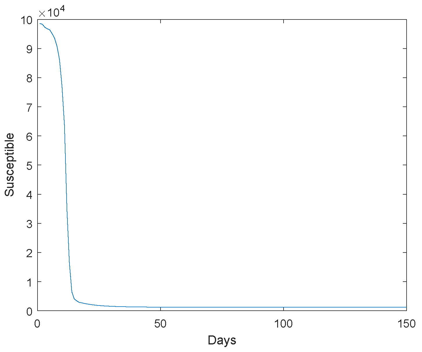
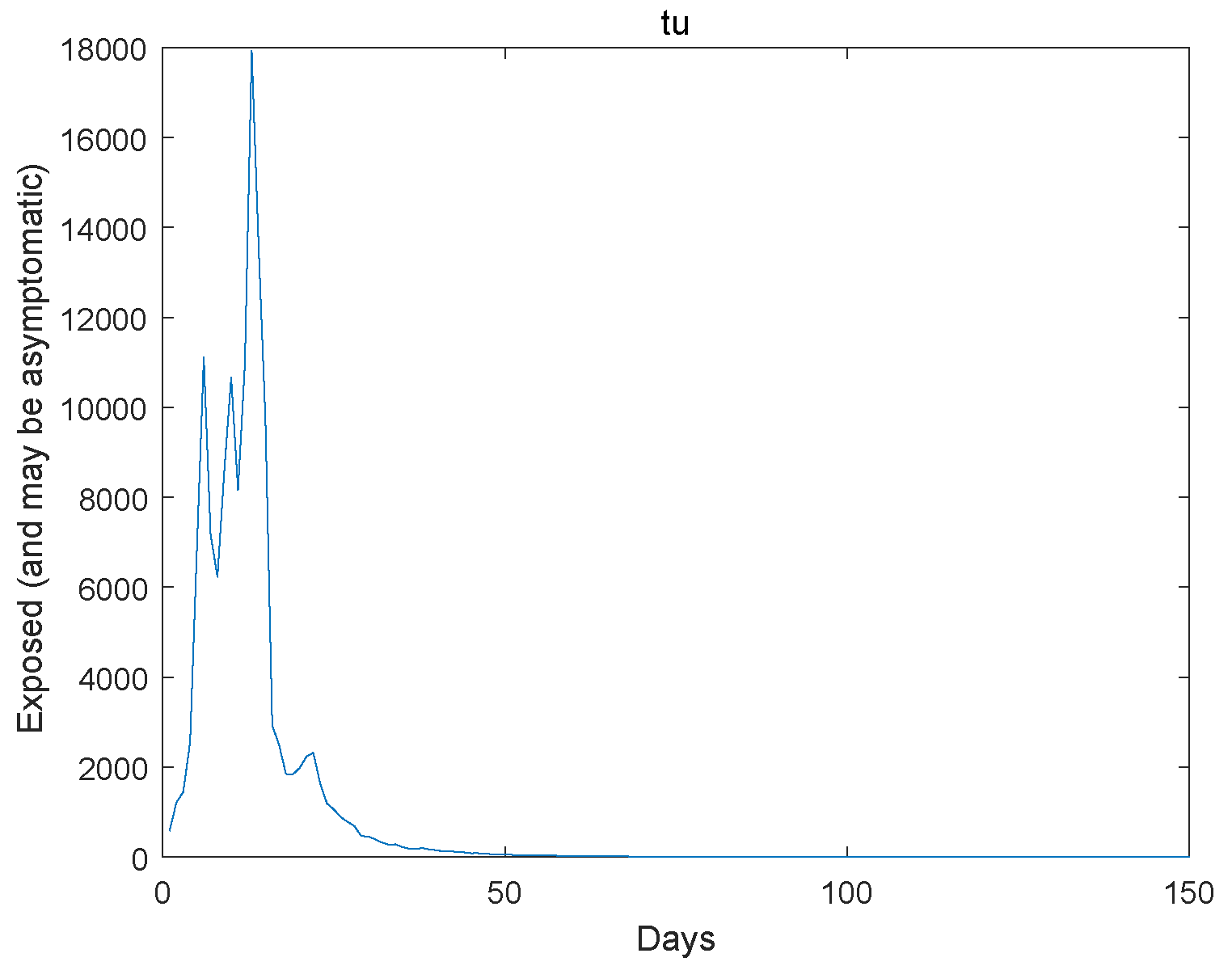
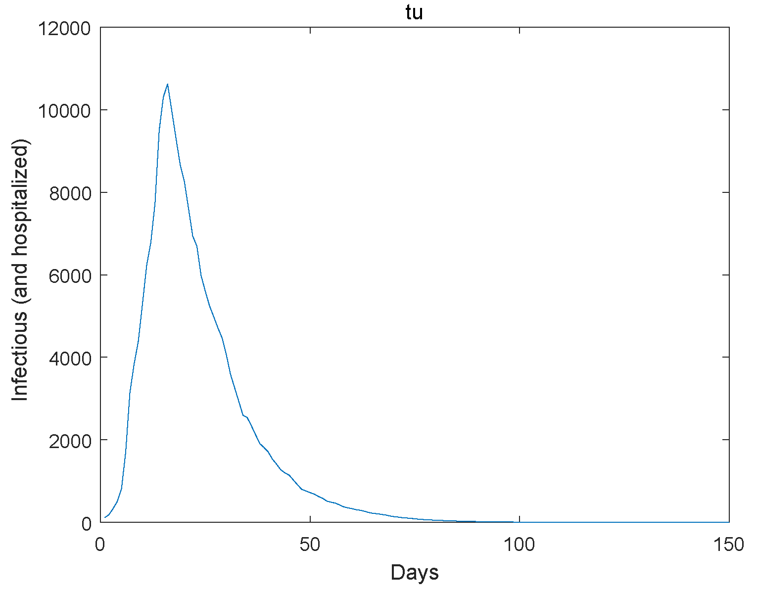
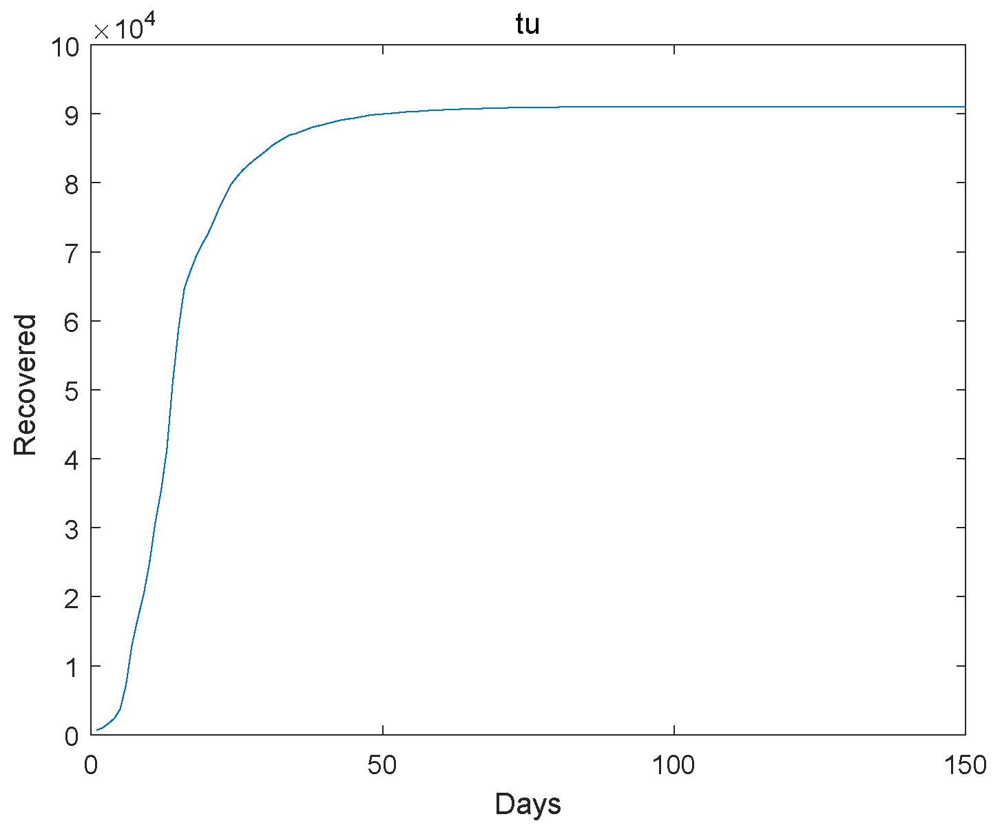
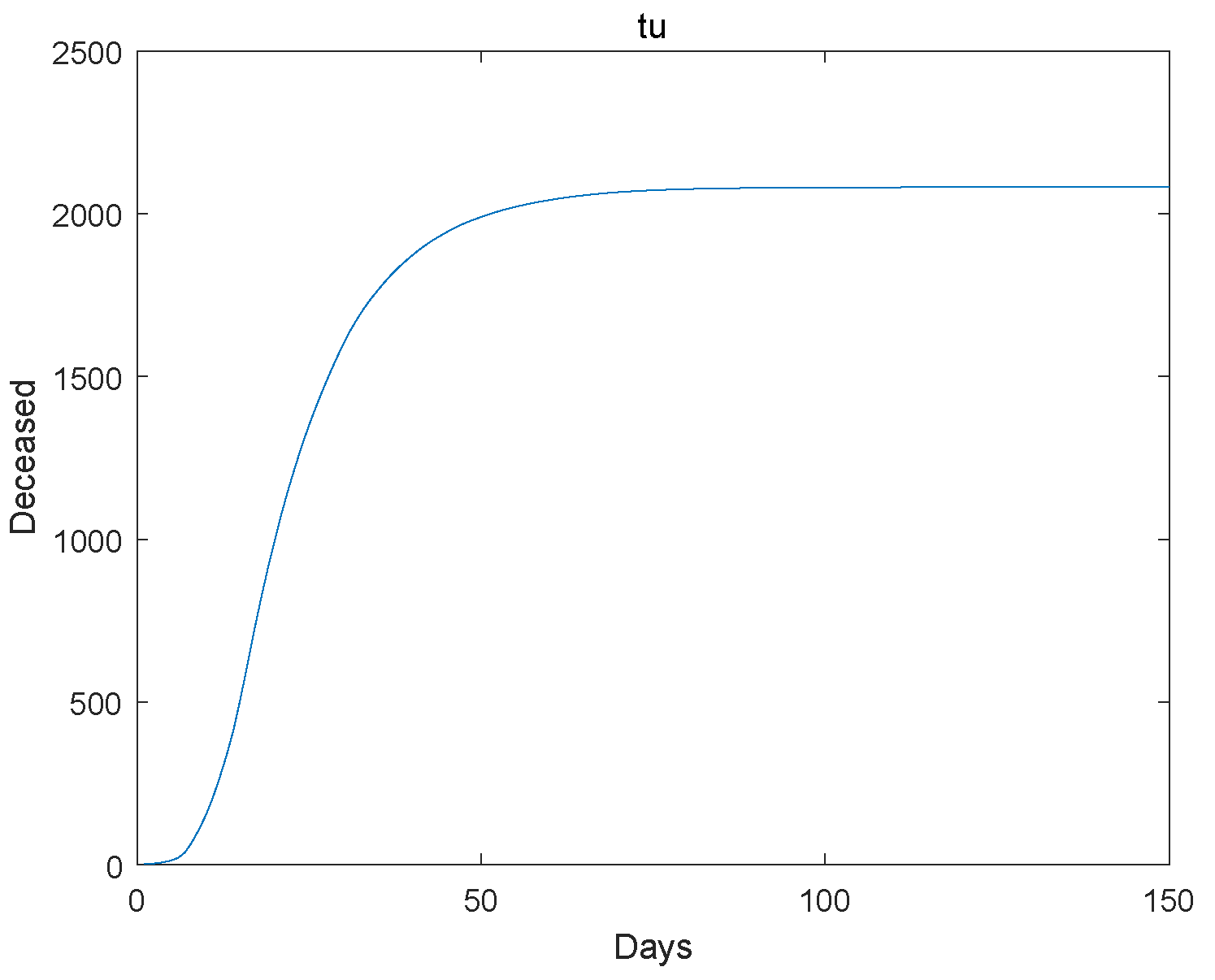
Based on the transmission characteristics of the disease and the research objectives, initially estimate the parameters in the model or set a reasonable initial range. Collect relevant infectious disease outbreak data, and we use the Markov Chain Monte Carlo simulation as utilized in reference [23] to estimate the model parameters using the Wuhan outbreak data. Next, we give the extinction of the system. The initial value , , , , , , , , . The Figure 1, Figure 2, Figure 3, Figure 4 and Figure 5 represent the simulation of progression of the number of individuals who are classified as susceptible, exposed, infectious, recovered, and deceased, plotted against the number of days.
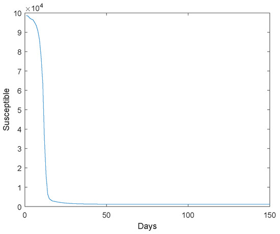
Figure 1.
The susceptible go to extinction.
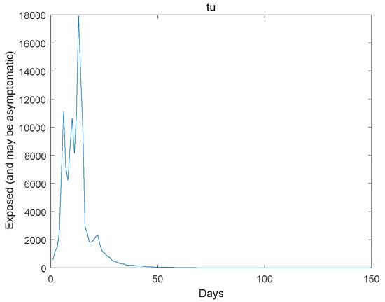
Figure 2.
The exposed go to extinction.
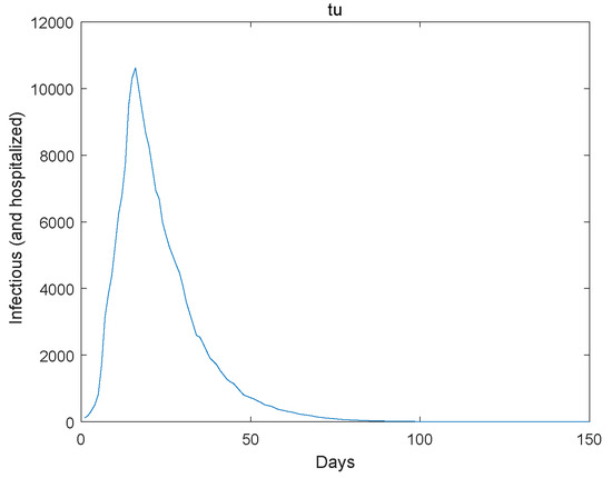
Figure 3.
The infectious go to extinction.

Figure 4.
The recovered go to extinction.
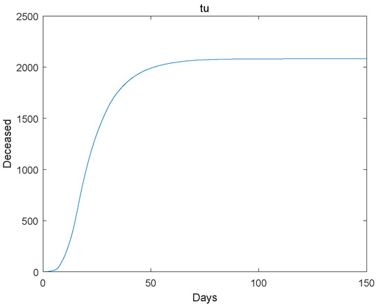
Figure 5.
The deceased go to extinction.
Remark 2.
Under the current parameter settings, the disease cannot sustain transmission within the population and will eventually disappear. This may be due to a relatively high recovery rate or a relatively low infection rate, resulting in a transmission rate insufficient to maintain the disease’s spread among people. The birth rate being relatively low may help reduce the number of new susceptible individuals, thereby slowing the transmission of the disease.
Remark 3.
The first perturbation coefficient being relatively high might imply that the conversion of susceptible individuals to infected individuals occurs rapidly; however, due to the configuration of other parameters, this does not lead to sustained transmission of the disease. This information is significant for understanding and controlling the spread of infectious diseases.
Remark 4.
It provides a mathematical proof that, given system dynamics, the total population does not grow indefinitely, but rather tends to stabilize over time. Although a disease control strategy is proposed in literature [12,13], this analysis of stability is not achieved by analyzing the ratio of each state in the system and the limit of the natural logarithm over time. Such stability analysis is crucial for understanding and predicting disease transmission and designing control strategies.
7. Conclusions
This study provides a mathematical foundation and theoretical support for understanding and predicting the transmission dynamics of COVID-19. It proves the existence of global solutions for the stochastic SEIRM COVID-19 model with a standard incidence rate. System stability is analyzed by constructing Lyapunov functions and employing relevant mathematical tools. The properties of the diffusion matrix are utilized to ensure the steady-state distribution of the system. The potential limitations of the model and the scope for future work have been discussed in more detail:
Understand that you need to reorganize the language for the following content [24,25,26,27,28]:
- Discuss whether the model assumes a uniform mixing of populations or fails to consider factors such as spatial distribution and varying contact rates among different demographic groups.
- If the model assumes constant parameters, this may be a limitation because real-world scenarios often involve time-varying parameters due to interventions or behavioral changes.
- Evaluate the model’s capacity to predict long-term outcomes in dynamic environments.
- Pandemics can be influenced by external factors such as policy changes, vaccine distribution, or the emergence of new variants.
- Consider unreported cases as potential limitations of the model. Additionally, propose that future research could build on this work by integrating methods to estimate and account for unreported cases.
Author Contributions
Methodology, D.W.; software, D.W.; writing—original draft preparation, Y.Z.; visualization, H.W. All authors have read and agreed to the published version of the manuscript.
Funding
This work was supported by program for National Natural Science Foundation of China (No.11526046).
Data Availability Statement
The original contributions presented in the study are included in the article, further inquiries can be directed to the corresponding authors.
Conflicts of Interest
The authors declare no conflict of interest.
References
- Kermack, W.O.; McKendrick, A.G. A contribution to the mathematical theory of epidemics. Proc. R. Soc. Lond. Ser. Contain. Pap. Math. Phys. Character 1927, 115, 700–721. [Google Scholar]
- Brauer, F. Compartmental models in epidemiology. Math. Epidemiol. 2008, 19–79. [Google Scholar]
- Aybar, O. Biochemical models of SIR and SIRS: Effects of bilinear incidence rate on infection-free and endemic states. Chaos 2023, 33, 093120. [Google Scholar] [CrossRef]
- Wang, J.; Zhang, J.; Jin, Z. Analysis of an SIR model with bilinear incidence rate. Nonlinear Anal. Real World Appl. 2010, 14, 2390–2402. [Google Scholar] [CrossRef]
- Zhang, Q. On small-data solution of the chemotaxis-SIS epidemic system with bilinear incidence rate. Nonlinear Anal. Real World Appl. 2024, 77, 104063. [Google Scholar] [CrossRef]
- Mahmood, P.; Majid, E. Global dynamics of an epidemic model with standard incidence rate and vaccination strategy. Chaos Solitons Fractals 2018, 117, 192–199. [Google Scholar]
- Han, S.; Lei, C.; Zhang, X. Qualitative analysis on a diffusive SIRS epidemic model with standard incidence infection mechanism. Z. Angew. Math. Phys. 2021, 71, 190. [Google Scholar] [CrossRef]
- Wu, Z.; Jiang, D. Dynamics and Density Function of a Stochastic SICA Model of a Standard Incidence Rate with Ornstein-Uhlenbeck Process. Qual. Theory Dyn. Syst. 2014, 23, 219. [Google Scholar] [CrossRef]
- Guo, S.; Xue, Y.; Li, X. A novel analysis approach of uniform persistence for a COVID-19 model with quarantine and standard incidence rate. Quant. Biol. 2022. [Google Scholar]
- Guo, S.; He, M.; Cui, J. Global Stability of a Time-delayed Malaria Model with Standard Incidence Rate. Acta Math. Appl.-Sin.-Engl. Ser. 2023, 39, 211–221. [Google Scholar] [CrossRef]
- He, B.; Peng, Y.; Sun, K. SEIR modeling of the COVID-19 and its dynamics. Nonlinear Dyn. 2020, 101, 1667–1680. [Google Scholar] [CrossRef] [PubMed]
- Saroj, K.; Ahmed, N.U. Mathematical modeling and optimal intervention of COVID-19 outbreak. Quatitative Biol. 2021, 9, 84–92. [Google Scholar]
- Shengjie, L. Effects of non-pharmaceutical interventions to contain COVID-19 in China. Nature 2020, 585, 410–413. [Google Scholar]
- Zhao, Y.; Wang, L. Practical exponential stability of impulsive stochastic food chain system with time-varying delays. Mathematics 2023, 11, 147. [Google Scholar] [CrossRef]
- Zhao, Y.; Lin, H.; Qiao, X. Persistence, extinction and practical exponential stability of impulsive stochastic competition models with varying delays. AIMS Math. 2023, 8, 22643–22661. [Google Scholar] [CrossRef]
- Xu, H.; Zhu, Q.; Zheng, W. Exponential stability of stochastic nonlinear delay systems subject to multiple periodic impulses. IEEE Trans. Autom. Control. 2024, 69, 2621–2628. [Google Scholar] [CrossRef]
- Zhao, Y.; Wang, L. Asymptotic behavior of a stochastic three-species food chain model with time-varying delays. Period. Ocean. Univ. China 2023, 53, 132–136. [Google Scholar]
- Zhao, Y.; Wang, L.; Wang, Y. The Periodic Solutions to a Stochastic Two-Prey One-Predator Population Model with Impulsive Perturbations in a Polluted Environment. Methodol. Comput. Appl. Probab. 2021, 23, 859–872. [Google Scholar] [CrossRef]
- Khan, A.; Ikram, R.; Din, A.; Humphries, U.W.; Akgul, A. Stochastic COVID-19 SEIQ epidemic model with time-delay. Results Phys. 2021, 30, 104775. [Google Scholar] [CrossRef]
- Allen, L. An Introduction to Stochastic Epidemic Models; Springer: Berlin/Heidelberg, Germany, 2008. [Google Scholar]
- Yang, Q.; Zhang, X.; Jiang, D. Dynamical behavior of a stochastic food chain system with ornstein uhlenbeck Process. J. Nonlinear Sci. 2022, 32, 34. [Google Scholar] [CrossRef]
- Mao, X. Stochastic Differential Equations and Their Applications; Horwood: Chichester, UK, 1997. [Google Scholar]
- He, S.; Tang, S.; Rong, C. A discrete stochastic model of the COVID-19 outbreak: Forecast and control. Math. Biosci. Eng. 2020, 17, 2792–2804. [Google Scholar] [CrossRef] [PubMed]
- Pei, L.; Zhang, M. Long-Term Predictions of COVID-19 in Some Countries by the SIRD Model. Complexity 2021, 1, 6692678. [Google Scholar] [CrossRef]
- Beghi, E.; Helbok, R.; Ozturk, S.; Karadas, O.; Lisnic, V.; Grosu, O.; Kovács, T.; Dobronyi, L.; Bereczki, D.; Cotelli, M.S.; et al. Short- and long-term outcome and predictors in an international cohort of patients with neuro-COVID-19. Eur. J. Neurol. 2022, 29, 1663–1684. [Google Scholar] [CrossRef] [PubMed]
- El-Shabasy, R. Three waves changes, new variant strains, and vaccination effect against COVID-19 pandemic. Int. J. Biol. Macromol. 2022, 204, 161–168. [Google Scholar] [CrossRef] [PubMed]
- Liu, Z. Predicting the number of reported and unreported cases for the COVID-19 epidemics in China, South Korea, Italy, France, Germany and United Kingdom. J. Theor. Biol. 2021, 509, 110501. [Google Scholar] [CrossRef]
- Hamou, A. Analysis and dynamics of a mathematical model to predict unreported cases of COVID-19 epidemic in Morocco. Comp. Appl. Math. 2021, 41, 289. [Google Scholar] [CrossRef]
Disclaimer/Publisher’s Note: The statements, opinions and data contained in all publications are solely those of the individual author(s) and contributor(s) and not of MDPI and/or the editor(s). MDPI and/or the editor(s) disclaim responsibility for any injury to people or property resulting from any ideas, methods, instructions or products referred to in the content. |
© 2024 by the authors. Licensee MDPI, Basel, Switzerland. This article is an open access article distributed under the terms and conditions of the Creative Commons Attribution (CC BY) license (https://creativecommons.org/licenses/by/4.0/).