Impulsive Discrete Runge–Kutta Methods and Impulsive Continuous Runge–Kutta Methods for Nonlinear Differential Equations with Delayed Impulses

Abstract

In this paper, we study the asymptotical stability of the exact solutions of nonlinear impulsive differential equations with the Lipschitz continuous function $f(t,x)$ for the dynamic system and for the impulsive term Lipschitz continuous delayed functions $I_k$. In order to obtain numerical methods with a high order of convergence and that are capable of preserving the asymptotical stability of the exact solutions of these equations, impulsive discrete Runge–Kutta methods and impulsive continuous Runge–Kutta methods are constructed, respectively. For these different types of numerical methods, different convergence results are obtained and the sufficient conditions for asymptotical stability of these numerical methods are also obtained, respectively. Finally, some numerical examples are provided to confirm the theoretical results.

1. Introduction

Impulsive differential equations (IDEs) are widely applied in numerous fields of science and technology: theoretical physics, mechanics, population dynamics, pharmacokinetics, industrial robotics, chemical technology, biotechnology, economics, etc. (see [1,2,3,4,5] and references therein). Recently, there has been growing interest in the study of impulsive differential equations with delayed impulses (DEDIs) [5,6,7,8,9,10,11,12,13,14,15,16,17]. In particular, the stability of the exact solutions of DEDIs has been widely studied [5,6,7,8,9,10,11,12,13]. However, to the best of our knowledge, our present paper is the first paper to study the asymptotical stability of nonlinear DEDIs under Lipschitz conditions.

In recent years, the theory of numerical methods for IDEs has been developed rapidly. The convergence and stability of numerical methods for scalar linear IDEs [18,19,20], multidimensional linear IDEs [21], semi-linear IDEs [22], nonlinear IDEs [23,24,25,26,27,28,29], impulsive time-delay differential equations [30,31,32,33,34,35] and stochastic impulsive time-delay differential equations [36] have been studied. But little work has been conducted on numerical methods for DEDIs. In [37], we investigated asymptotical stability and convergence of impulsive discrete Runge–Kutta methods for linear DEDIs. In our present paper, we further investigate the convergence and stability of impulsive discrete Runge–Kutta methods for nonlinear DEDIs.

Continuous numerical methods are widely applied to delay differential equations without impulsive perturbations (see [38,39,40,41,42,43], etc.). But the exact solutions of impulsive differential equations are not continuous, so the continuous numerical methods are not applicable for impulsive differential equations. In [20], asymptotical stability and convergence of impulsive collocation methods for impulsive ordinary differential equations were studied. In [35], the convergence of the impulsive continuous Runge–Kutta methods was studied. As far as we know, our present paper is the first to study the convergence and stability of impulsive continuous Runge–Kutta methods (ICRKMs) for nonlinear DEDIs.

The Runge–Kutta method ([44,45,46,47]) is applicable to various types of ordinary differential equations and its advantages mainly include high accuracy, generally good numerical stability and convergence. A natural question is, when applying the Runge–Kutta method to solve DEDIs, does the Runge–Kutta method method still have good stability and convergence when we treat the impulse terms in different ways? The continuous Runge–Kutta method ([39,46]) is described above and is suitable for solving ordinary differential equations and delay differential equations. It is also important for many practical questions such as graphical output, and even location or treatment of discontinuities in differential equations. Another natural question is whether the application of the continuous Runge–Kutta method to solve DEDIs also has good stability and convergence. This paper will answer both of these questions.

The remainder of this paper is arranged as follows. In Section 2, sufficient conditions for asymptotical stability of the exact solution of a class of nonlinear DEDIs are provided. In Section 3, the scheme 1 are correct. impulsive Runge–Kutta methods (S1IRKMs) are constructed. It is proved that S1IRKM is convergent of order p if the corresponding Runge–Kutta method is p-th order. S1IRKMs are obtained to preserve asymptotical stability of the exact solutions under the sufficient conditions obtained in Section 2, applying the theory of Padé approximation. Moreover, the scheme 1 impulsive $\theta$ method (S1I$\theta$M) are obtained to preserve asymptotical stability of the exact solutions under the sufficient conditions. In Section 4, the scheme 2 impulsive Runge–Kutta methods (S2IRKM) are constructed. It is proved that S2IRKM is only convergent of order 1 if the corresponding Runge–Kutta method is p-th order. S2IRKMs are obtained to preserve asymptotical stability of the exact solutions under the sufficient conditions applying the theory of Padé approximation. Moreover, the scheme 2 impulsive $\theta$ method (S2I$\theta$M) is obtained to preserve asymptotical stability of the exact solutions under sufficient conditions. In Section 5, the convergence and asymptotical stability of ICRKMs are studied. In Section 6, we provide two numerical examples to confirm our theoretical results. Finally, in Section 7, conclusions and future work are provided.

2. Asymptotical Stability of the Exact Solutions of DEDIs

Consider the DEDI [6] of the following form

$$\left\{\begin{array}{cc}{x}^{\prime }\left(t\right)=f(t,x\left(t\right)),\hfill & t\ge t_0,t\ne {\tau }_k,k\in {\mathbb{Z}}^{+},\hfill \\ x\left({\tau }_k^{+}\right)=I_k\left(x\left(r_k^{-}\right)\right),\hfill & r_k\in {\mathcal{F}}_{{\tau }_k}^{\sigma },k\in {\mathbb{Z}}^{+},\hfill \\ x\left(t_0\right)=x_0,\hfill \end{array}\right.$$

(1)

where ${\mathbb{Z}}^{+}=\{1,2,\cdots \}$, $x\left(t^{+}\right)$ is the right limit of $x\left(t\right)$, $t_0={\tau }_0<{\tau }_1<{\tau }_2<\cdots$, ${lim}_{k\to \infty }{\tau }_k=\infty$, the function $f:[t_0,+\infty )\times {\mathbb{R}}^d\to {\mathbb{R}}^d$ is continuous in t and Lipschitz continuous with respect to the second variable in the following sense: there is a positive real constant $\alpha$ such that

$$\parallel f(t,x_1)-f(t,x_2)\parallel \le \alpha \parallel x_1-x_2\parallel$$

(2)

for arbitrary $t\in [t_0,\infty )$, $x_1,x_2\in {\mathbb{R}}^d$, where $\parallel ·\parallel$ is any convenient norm on ${\mathbb{R}}^d$. Define the functions $I_k$ to be from ${\mathbb{R}}^d$ to ${\mathbb{R}}^d$, $k\in {\mathbb{Z}}^{+}$. Assume that each function $I_k$ ($k\in {\mathbb{Z}}^{+}$ ) is Lipschitz continuous, i.e., there is a positive constant ${\beta }_k$ such that

$$\parallel I_k\left(x\right)-I_k\left(y\right)\parallel \le {\beta }_k\parallel x-y\parallel ,\mathrm{for}\forall x,y\in {\mathbb{R}}^d.$$

(3)

For any given impulse sequence ${\tau }_k$, $k\in {\mathbb{Z}}^{+}$ and any constant $\sigma \in (0,1]$, the set ${\mathcal{F}}_{{\tau }_k}^{\delta }$ is defined as follows

$${\mathcal{F}}_{{\tau }_k}^{\sigma }=\{r_k:r_k=(1-\sigma ){\tau }_{k-1}+\sigma {\tau }_k,k\in {\mathbb{Z}}^{+}\}.$$

Definition 1. 

A function $x:[t_0,\infty )\to {\mathbb{R}}^d$ is said to be a solution of (1), if

(i) 

$\underset{t\to t_0^{+}}{lim}x\left(t\right)=x_0$,

(ii) 

For $t\in (t_0,+\infty ),t\ne {\tau }_k,k=1,2,\cdots$, $x\left(t\right)$ is differentiable and $x^{\prime }\left(t\right)=f(t,x\left(t\right))$,

(iii) 

$x\left(t\right)$ is right continuous in $(t_0,+\infty )$ and $x\left({\tau }_k\right)=I_k\left(x\left(r_k^{-}\right)\right),k=1,2,\cdots$.

In order to investigate the asymptotical stability of $x\left(t\right)$, consider Equation (1) with another initial datum:

$$\left\{\begin{array}{c}{y}^{\prime }\left(t\right)=f(t,y\left(t\right)),t>t_0,t\ne {\tau }_k,k\in {\mathbb{Z}}^{+},\hfill \\ y\left({\tau }_k\right)=I_k\left(y\left(r_k^{-}\right)\right),r_k\in {\mathcal{F}}_{{\tau }_k}^{\delta },k\in {\mathbb{Z}}^{+},\hfill \\ y\left(t_0\right)=y_0.\hfill \end{array}\right.$$

(4)

Definition 2. 

The exact solution $x\left(t\right)$ of (1) is said to be

1. 

stable if, for an arbitrary $ϵ>0$, there exists a positive number $\delta =\delta \left(ϵ\right)$ such that, for any other solution $y\left(t\right)$ of (4), $\parallel x_0-y_0\parallel <\delta$ implies

$$\parallel x\left(t\right)-y\left(t\right)\parallel <ϵ,\forall t>t_0;$$

2. 

asymptotically stable, if it is stable and $\underset{t\to \infty }{lim}\parallel x\left(t\right)-y\left(t\right)\parallel =0.$

Theorem 1. 

Assume that there exists a positive constant γ such that ${\tau }_k-{\tau }_{k-1}\le \gamma$, $k\in {\mathbb{Z}}^{+}$. The exact solution of (1) is asymptotically stable if there is a positive constant C such that

$${\beta }_k{\mathrm{e}}^{\alpha \sigma ({\tau }_k-{\tau }_{k-1})}\le C<1$$

(5)

for arbitrary $k\in {\mathbb{Z}}^{+}$.

Proof. 

For arbitrary $t\in [{\tau }_k,{\tau }_{k+1})$, $k=0,1,2,\cdots$, we can obtain that

$$\begin{array}{cc}\hfill \parallel x\left(t\right)-y\left(t\right)\parallel & =\parallel x\left({\tau }_k\right)-y\left({\tau }_k\right)+{\int }_{{\tau }_{k-1}}^t(f(s,x\left(s\right))-f(s,y\left(s\right)))ds\parallel \hfill \\ \hfill & \le \parallel x\left({\tau }_k\right)-y\left({\tau }_k\right)\parallel +{\int }_{{\tau }_k}^t\parallel f(s,x\left(s\right))-f(s,y\left(s\right))\parallel ds\hfill \\ \hfill & \le \parallel x\left({\tau }_k\right)-y\left({\tau }_k\right)\parallel +\alpha {\int }_{{\tau }_k}^t\parallel x\left(s\right)-y\left(s\right)\parallel ds\hfill \end{array}$$

By Gronwall’s Theorem, for arbitrary $t\in [{\tau }_k,{\tau }_{k+1})$, $k=0,1,2,\cdots$, we have

$$\parallel x\left(t\right)-y\left(t\right)\parallel \le \parallel x\left({\tau }_k\right)-y\left({\tau }_k\right)\parallel {\mathrm{e}}^{\alpha (t-{\tau }_k)},$$

which implies

$$\parallel x\left(r_{k+1}^{-}\right)-y\left(r_{k+1}^{-}\right)\parallel \le \parallel x\left({\tau }_k\right)-y\left({\tau }_k\right)\parallel {\mathrm{e}}^{\alpha (r_{k+1}-{\tau }_k)}=\parallel x\left({\tau }_k\right)-y\left({\tau }_k\right)\parallel {\mathrm{e}}^{\alpha \sigma ({\tau }_{k+1}-{\tau }_k)}.$$

Consequently, we can obtain that

$$\begin{array}{cc}\hfill & \parallel x\left({\tau }_{k+1}\right)-y\left({\tau }_{k+1}\right)\parallel \hfill \\ & =\parallel I_{k+1}\left(x\left(r_{k+1}^{-}\right)\right)-I_{k+1}\left(y\left(r_{k+1}^{-}\right)\right)\parallel \hfill \\ \hfill & \le {\beta }_{k+1}\parallel x\left(r_{k+1}^{-}\right)-y\left(r_{k+1}^{-}\right)\parallel \hfill \\ \hfill & \le \parallel x\left({\tau }_k\right)-y\left({\tau }_k\right)\parallel {\beta }_{k+1}{\mathrm{e}}^{\alpha \sigma ({\tau }_{k+1}-{\tau }_k)}.\hfill \end{array}$$

Therefore, by the method of introduction and the conditions (3) and (5), for arbitrary $t\in [{\tau }_k,{\tau }_{k+1})$, $k=0,1,2,\cdots$, we can obtain that

$$\begin{array}{cc}\hfill & \parallel x\left(t\right)-y\left(t\right)\parallel \hfill \\ & \le \parallel x_0-y_0\parallel {\mathrm{e}}^{\alpha (t-{\tau }_k)}\prod _{i=1}^k{\beta }_i{\mathrm{e}}^{\alpha \sigma ({\tau }_i-{\tau }_{i-1})}\hfill \\ \hfill & \le C^k\parallel x_0-y_0\parallel {\mathrm{e}}^{\alpha (t-{\tau }_k)}\hfill \\ \hfill & \le C^k\parallel x_0-y_0\parallel {\mathrm{e}}^{\alpha ({\tau }_{k+1}-{\tau }_k)}\hfill \\ \hfill & \le C^k\parallel x_0-y_0\parallel {\mathrm{e}}^{\alpha \gamma },\hfill \end{array}$$

which implies $\parallel x\left({\tau }_{k+1}^{-}\right)-y\left({\tau }_{k+1}^{-}\right)\parallel \le C^k\parallel x_0-y_0\parallel {\mathrm{e}}^{\alpha \gamma }$ and $\parallel x\left({\tau }_{k+1}\right)-y\left({\tau }_{k+1}\right)\parallel \le \parallel x_0-y_0\parallel C^{k+1}$. Hence for an arbitrary $ϵ>0$, there exists $\delta ={\mathrm{e}}^{-\alpha \gamma }ϵ$ such that $\parallel x_0-y_0\parallel <\delta$ implies

$$\parallel x\left(t\right)-y\left(t\right)\parallel \le C^k\parallel x_0-y_0\parallel {\mathrm{e}}^{\alpha \gamma }\le \parallel x_0-y_0\parallel {\mathrm{e}}^{\alpha \gamma }<ϵ$$

for arbitrary $t\in [{\tau }_k,{\tau }_{k+1})$, $k=0,1,2,\cdots$, i.e.,

$$\parallel x\left(t\right)-y\left(t\right)\parallel <ϵ,\forall t>t_0.$$

So the exact solution of (1) is stable. Obviously, for arbitrary $t\in [{\tau }_k,{\tau }_{k+1})$, $k=0,1,2,\cdots$,

$$\parallel x\left(t\right)-y\left(t\right)\parallel \le C^k\parallel x_0-y_0\parallel {\mathrm{e}}^{\alpha \gamma }\to 0,k\to \infty .$$

Similarly, we can also obtain that

$$\parallel x\left({\tau }_{k+1}^{-}\right)-y\left({\tau }_{k+1}^{-}\right)\parallel \le C^k\parallel x_0-y_0\parallel {\mathrm{e}}^{\alpha \gamma }\to 0,k\to \infty ,$$

and

$$\parallel x\left({\tau }_{k+1}^{+}\right)-y\left({\tau }_{k+1}^{+}\right)\parallel \le C^{k+1}\parallel x_0-y_0\parallel \to 0,k\to \infty .$$

Consequently, the exact solution of (1) is asymptotically stable. □

From the proof of Theorem 1, we can obtain the following result.

Remark 1. 

If condition (5) of Theorem 1 is changed into the weaker condition

$${\beta }_k{\mathrm{e}}^{\alpha \sigma ({\tau }_k-{\tau }_{k-1})}\le 1,\forall k\in {\mathbb{Z}}^{+},$$

(6)

then the exact solution of (1) is stable.

3. Scheme 1 Impulsive Discrete Runge–Kutta Methods

In the following part of this paper, we will focus on the case of $0<\sigma <1$; the special case of $\sigma =1$ has already been studied in paper [29]. The simplest and most straightforward idea is to take all points in the set $\{{\tau }_k,r_k:{\mathbb{Z}}^{+}\}$ as the numerical mesh. For convenience, we divide the intervals $[{\tau }_{k-1},r_k]$ and $[r_k,{\tau }_k)$ ($k\in {\mathbb{Z}}^{+}$) equally by m; m is a positive integer. In this case, for $k\in \mathbb{N}$, the step sizes are as follows

$$h_{k,l}=\left\{\begin{array}{cc}{\overline{h}}_{k,1}:={\displaystyle \frac{r_k-{\tau }_k}{m}},\hfill & l=1,2,\cdots ,m\hfill \\ {\overline{h}}_{k,2}:={\displaystyle \frac{{\tau }_{k+1}-r_k}{m}},\hfill & l=m+1,m+2,\cdots ,2m,\hfill \end{array}\right.$$

(7)

which implies that the mesh point $t_{k,0}={\tau }_k$, $t_{k,2m}={\tau }_{k+1}^{-}$, $t_{k,l}={\tau }_k+{\sum }_{j=0}^l{h}_{k,j}$, $\forall k\in \mathbb{N}$, $l=1,2,\cdots ,2m-1$.

The S1IRKM for DEDI (1) can be constructed as follows:

$$\left\{\begin{array}{cc}{X}_{k,l+1}^i=x_{k,l}+h_{k,l+1}{\displaystyle \sum _{j=1}^v}{a}_{ij}f(t_{k,l+1}^j,X_{k,l+1}^j),\hfill & k\in \mathbb{N},i=1,2,\cdots ,v,\hfill \\ x_{k,l+1}=x_{k,l}+h_{k,l+1}{\displaystyle \sum _{i=1}^v}{b}_{i}f(t_{k,l+1}^i,X_{k,l+1}^i),\hfill & l=0,1,\cdots ,2m-1,\hfill \\ x_{k+1,0}=I_{k+1}\left(x_{k,m}\right),\hfill \\ x_{0,0}=x_0,\hfill \end{array}\right.$$

(8)

where v is referred to as the number of stages, $t_{k,l}^i=t_{k,l}+c_i{h}_{k,l+1}$, $x_{k,l}$ is an approximation to the exact solution $x\left(t_{k,l}\right)$ and $X_{k,l+1}^i$ is an approximation to the exact solution $x\left(t_{k,l+1}^i\right)$, $k\in \mathbb{N},l=0,1,\cdots ,2m-1,i=1,2,\cdots ,v$. The weights $b_i$, the abscissae $c_i={\displaystyle \sum _{j=1}^v}{a}_{ij}$ and the matrix $A={\left[a_{ij}\right]}_{i,j=1}^v$ will be denoted by $(A,b,c)$.

3.1. Convergence of S1IRKMs

In order to study the convergence of S1IRKMs, the DEDI (1) is restricted to the interval $[0,T]$ in this subsection. For convenience, assume that there exists a positive integer N such that $T={\tau }_N$.

To analyze the local truncation errors of S1IRKM (8) for DEDI (1), consider the following local problem

$$\left\{\begin{array}{cc}{Z}_{k,l+1}^i=z_{k,l}+h_{k,l+1}{\displaystyle \sum _{j=1}^v}{a}_{ij}f(t_{k,l+1}^j,Z_{k,l+1}^j),\hfill & k\in \mathbb{N},i=1,2,\cdots ,v,\hfill \\ z_{k,l+1}=z_{k,l}+h_{k,l+1}{\displaystyle \sum _{i=1}^v}{b}_{i}f(t_{k,l+1}^i,Z_{k,l+1}^i),\hfill & l=0,1,\cdots ,2m-1,\hfill \end{array}\right.$$

(9)

where $z_{k,l}=x\left(t_{k,l}\right)$, $k=0,1,2,\cdots ,N-1$, $l=0,1,2,\cdots ,2m-1$.

Because it can be seen as a problem of ordinary differential equation (see [44,45,46]) when we consider the local problem, we can directly obtain the following result.

Theorem 2. 

Consider the DEDI (1) where $f(t,x)$ is $C^p$-continuous in $[t_0,T]\times {\mathbb{R}}^d$. If the corresponding Runge–Kutta method is convergent of order p, then local errors between the numerical solutions obtained from (9) and the exact solutions obtained from DEDI (1) satisfy that there exists a constant C such that, for arbitrary $k=0,1,2,\cdots ,N-1$, $l=0,1,2,\cdots ,2m-2$,

$$R_{k,l+1}:=\parallel z_{k,l+1}-x\left(t_{k,l+1}\right)\parallel \le C{h}_{k,l+1}^{p+1}$$

and

$$R_{k,2m}:=\parallel z_{k,2m}-x\left({\tau }_{k+1}^{-}\right)\parallel \le C{h}_{k,2m}^{p+1}.$$

Theorem 3. 

Assume that $f(t,x)$ of DEDI (1) is $C^p$-continuous in $[t_0,T]\times {\mathbb{R}}^d$, the functions $I_k$ are bounded, and Lipschitz conditions (2) and (3) hold. If the corresponding Runge–Kutta method is convergent of order p, then the global errors $e_{k,l}$ between the numerical solutions $x_{k,l}$ obtained from (8) and the exact solutions $x\left(t_{k,l}\right)$ obtained from DEDI (1) satisfy that there exists a constant $C_1$ such that, when h is small enough, for arbitrary $k=0,1,2,\cdots ,N-1$, $l=0,1,2,\cdots ,2m-1$,

$$e_{k,l}:=\parallel x_{k,l}-x\left(t_{k,l}\right)\parallel \le C_1{h}^p$$

(10)

and

$$e_{k,2m}:=\parallel x_{k,2m}-x\left({\tau }_{k+1}^{-}\right)\parallel \le C_1{h}^p,$$

(11)

where $h=\underset{k,l}{max}\left\{h_{k,l}\right\}=\underset{k}{max}\{{\overline{h}}_{k,1},{\overline{h}}_{k,2}\}$.

Proof. 

From (8) and (9), we can obtain that

$$\begin{array}{cc}\hfill & \parallel X_{k,l+1}^i-Z_{k,l+1}^i\parallel \hfill \\ \hfill & =\parallel x_{k,l}-z_{k,l}+h_{k,l+1}\sum _{j=1}^v{a}_{ij}(f(t_{k,l+1}^j,X_{k,l+1}^j)-f(t_{k,l+1}^j,Z_{k,l+1}^j))\parallel \hfill \\ \hfill & \le \parallel x_{k,l}-z_{k,l}\parallel +h_{k,l+1}\sum _{j=1}^v|a_{ij}|\parallel f(t_{k,l+1}^j,X_{k,l+1}^j)-f(t_{k,l+1}^j,Z_{k,l+1}^j)\parallel \hfill \\ \hfill & \le \parallel x_{k,l}-z_{k,l}\parallel +\alpha h_{k,l+1}\sum _{j=1}^v|a_{ij}|\parallel X_{k,l+1}^j-Z_{k,l+1}^j\parallel \hfill \\ \hfill & \le \parallel x_{k,l}-z_{k,l}\parallel +\alpha h\left(\underset{1\le i\le v}{max}\sum _{j=1}^v|a_{ij}|\right)\underset{1\le j\le v}{max}\{\parallel X_{k,l+1}^j-Z_{k,l+1}^j\parallel \}\hfill \end{array}$$

which implies that, for $h<{\alpha }^{-1}{\left({max}_{1\le i\le v}{\sum }_{j=1}^v|a_{ij}|\right)}^{-1}$,

$$\underset{1\le i\le v}{max}\{\parallel X_{k,l+1}^i-Z_{k,l+1}^i\parallel \}\le {\Lambda }_1\parallel x_{k,l}-z_{k,l}\parallel .$$

where $\Lambda ={\left(1-\alpha h\left(\underset{1\le i\le v}{max}{\sum }_{j=1}^v|a_{ij}|\right)\right)}^{-1}$. Hence,

$$\begin{array}{cc}\hfill & \parallel x_{k,l+1}-z_{k,l+1}\parallel \hfill \\ \hfill & =\parallel x_{k,l}-z_{k,l}+h_{k,l+1}\sum _{j=1}^v{b}_j(f(t_{k,l+1}^j,X_{k,l+1}^j)-f(t_{k,l}^j,Z_{k,l}^j))\parallel \hfill \\ \hfill & \le \parallel x_{k,l}-z_{k,l}\parallel +h_{k,l+1}\sum _{j=1}^v|b_j|\parallel f(t_{k,l+1}^j,X_{k,l+1}^j)-f(t_{k,l+1}^j,Z_{k,l+1}^j)\parallel \hfill \\ \hfill & \le \parallel x_{k,l}-z_{k,l}\parallel +\alpha h_{k,l+1}\left(\sum _{j=1}^v|b_j|\right)\underset{1\le i\le v}{max}\{\parallel X_{k,l+1}^i-Z_{k,l+1}^i\parallel \}\hfill \\ \hfill & \le \left(1+\alpha B\Lambda h_{k,l+1}\right)\parallel x_{k,l}-z_{k,l}\parallel \hfill \end{array}$$

where $B={\displaystyle \sum _{j=1}^v}|b_j|$. From Theorem 2, we have

$$\begin{array}{cc}\hfill & {\overline{R}}_{k,1}:=\underset{1\le l\le m}{max}{R}_{k,l}\le C{\overline{h}}_{k,1}{h}^p,\hfill \\ \hfill /& {\overline{R}}_{k,2}:=\underset{m+1\le l\le 2m}{max}{R}_{k,l}\le C{\overline{h}}_{k,2}{h}^p.\hfill \end{array}$$

If $0\le l\le m-1$,

$$\begin{array}{cc}{e}_{k,l+1}\hfill & :=\parallel x\left(t_{k,l+1}\right)-x_{k,l+1}\parallel \hfill \\ \hfill & \le \parallel x\left(t_{k,l+1}\right)-z_{k,l+1}\parallel +\parallel z_{k,l+1}-x_{k,l+1}\parallel \hfill \\ \hfill & \le \left(1+\alpha B\Lambda {\overline{h}}_{k,1}\right)e_{k,l}+{\overline{R}}_{k,1}\hfill \\ \hfill & \le {\left(1+\alpha B\Lambda {\overline{h}}_{k,1}\right)}^{l+1}{e}_{k,0}+\left({\left(1+\alpha B\Lambda {\overline{h}}_{k,1}\right)}^{l+1}-1\right){\displaystyle \frac{{\overline{R}}_{k,1}}{\alpha \beta \Lambda {\overline{h}}_{k,1}}}\hfill \\ \hfill & \le {\mathrm{e}}^{(l+1)\alpha B\Lambda {\overline{h}}_{k,1}}{e}_{k,0}+\left({\mathrm{e}}^{(l+1)\alpha B\Lambda {\overline{h}}_{k,1}}-1\right){\displaystyle \frac{{\overline{R}}_{k,1}}{\alpha B\Lambda {\overline{h}}_{k,1}}}\hfill \\ \hfill & \le {\mathrm{e}}^{\alpha B\Lambda \sigma ({\tau }_{k+1}-{\tau }_k)}{e}_{k,0}+\left({\mathrm{e}}^{\alpha B\Lambda \sigma ({\tau }_{k+1}-{\tau }_k)}-1\right){\displaystyle \frac{C{h}^p}{\alpha B\Lambda }}\hfill \\ \hfill & \le {\mathrm{e}}^{\alpha B\Lambda \sigma T}{e}_{k,0}+\left({\mathrm{e}}^{\alpha B{\Lambda }_1\sigma T}-1\right){\displaystyle \frac{C{h}^p}{\alpha B\Lambda }}\hfill \end{array}$$

(12)

Otherwise, if $m\le l\le 2m-1$,

$$\begin{array}{cc}{e}_{k,l+1}\hfill & :=\parallel x\left(t_{k,l+1}\right)-x_{k,l+1}\parallel \hfill \\ \hfill & \le \parallel x\left(t_{k,l+1}\right)-z_{k,l+1}\parallel +\parallel z_{k,l+1}-x_{k,l+1}\parallel \hfill \\ \hfill & \le \left(1+\alpha B\Lambda {\overline{h}}_{k,2}\right)e_{k,l}+{\overline{R}}_{k,2}\hfill \\ \hfill & \le {\left(1+\alpha B\Lambda {\overline{h}}_{k,2}\right)}^{l-m+1}{e}_{k,m}+\left({\left(1+\alpha B\Lambda {\overline{h}}_{k,2}\right)}^{l-m+1}-1\right){\displaystyle \frac{{\overline{R}}_{k,2}}{\alpha B\Lambda {\overline{h}}_{k,2}}}\hfill \\ \hfill & \le {\mathrm{e}}^{(l-m+1)\alpha B\Lambda {\overline{h}}_{k,2}}{e}_{k,m}+\left({\mathrm{e}}^{(l-m+1)\alpha B\Lambda {\overline{h}}_{k,2}}-1\right){\displaystyle \frac{{\overline{R}}_{k,2}}{\alpha \beta \Lambda {\overline{h}}_{k,2}}}\hfill \\ \hfill & \le {\mathrm{e}}^{\alpha B\Lambda (1-\sigma )({\tau }_{k+1}-{\tau }_k)}{e}_{k,m}+\left({\mathrm{e}}^{\alpha B\Lambda (1-\sigma )({\tau }_{k+1}-{\tau }_k)}-1\right){\displaystyle \frac{C{h}^p}{\alpha \beta \Lambda }}\hfill \\ \hfill & \le {\mathrm{e}}^{\alpha B\Lambda (1-\sigma )T}{e}_{k,m}+\left({\mathrm{e}}^{\alpha B\Lambda (1-\sigma )T}-1\right){\displaystyle \frac{C{h}^p}{\alpha B\Lambda }}\hfill \\ \hfill & \le {\mathrm{e}}^{\alpha B\Lambda T}{e}_{k,0}+\left({\mathrm{e}}^{\alpha B\Lambda T}-1\right){\displaystyle \frac{C{h}^p}{\alpha B\Lambda }}\hfill \end{array}$$

(13)

Otherwise,

$$\begin{array}{cc}{e}_{k+1,0}\hfill & :=\parallel x_{k+1,0}-x\left(t_{k+1,0}\right)\parallel =\parallel x_{k+1,0}-x\left({\tau }_{k+1}\right)\parallel \hfill \\ \hfill & =\parallel I_{k+1}\left(x_{k,m}\right)-I_{k+1}\left(x\left({\tau }_{k+1}^{-}\right)\right)\parallel \hfill \\ \hfill & \le {\beta }_{k+1}\parallel x_{k,m}-x\left(t_{k,m}^{-}\right)\parallel \hfill \\ \hfill & \le {\beta }_{k+1}{\mathrm{e}}^{\alpha B\Lambda \sigma T}{e}_{k,0}+{\beta }_{k+1}\left({\mathrm{e}}^{\alpha B\Lambda \sigma T}-1\right){\displaystyle \frac{C{h}^p}{\alpha B\Lambda }}\hfill \\ \hfill & \le \overline{B}{\mathrm{e}}^{\alpha B\Lambda \sigma T}{e}_{k,0}+\overline{B}\left({\mathrm{e}}^{\alpha B\Lambda \sigma T}-1\right){\displaystyle \frac{C{h}^p}{\alpha B\Lambda }}\hfill \\ \hfill & \le {\left(\overline{B}{\mathrm{e}}^{\alpha B\Lambda \sigma T}\right)}^{k+1}{e}_{0,0}+\left({\left(\overline{B}{\mathrm{e}}^{\alpha B\Lambda \sigma T}\right)}^{k+1}-1\right){\displaystyle \frac{C{h}^p}{\alpha B\Lambda }},\hfill \end{array}$$

(14)

where $\overline{B}=max\{{\beta }_1,{\beta }_2,\cdots ,{\beta }_N\}$. In fact, we can choose $\parallel x_{0,0}-x_0\parallel =O\left(h^p\right))$; that is, $\parallel e_{0,0}\parallel =O\left(h^p\right)$. For convenience, we only choose $x_{0,0}=x_0$, which impiles that $e_{0,0}=0$. So from (14), for arbitrary $k=0,1,2,\dots ,N$, we have

$$e_{k+1,0}\le C_2{h}^p$$

(15)

where $C_2=\left({\left(\overline{B}{\mathrm{e}}^{\alpha B\Lambda \sigma T}\right)}^N-1\right){\displaystyle \frac{C}{\alpha B\Lambda }}$. Combining (12) and (15), for $0\le l\le m-1$, we can obtain that

$$e_{k,l+1}\le C_3{h}^p$$

(16)

where $C_3={\mathrm{e}}^{\alpha B\Lambda \sigma T}{C}_2+\left({\mathrm{e}}^{\alpha B\Lambda \sigma T}-1\right){\displaystyle \frac{C}{\alpha B\Lambda }}$. Similarly, combining (13) and (16), for $m\le l\le 2m-1$, we obtain

$$e_{k,l+1}\le C_4{h}^p$$

(17)

where $C_4={\mathrm{e}}^{\alpha B\Lambda T}{C}_2+\left({\mathrm{e}}^{\alpha B\Lambda T}-1\right){\displaystyle \frac{C{h}^p}{\alpha B\Lambda }}$. Consequently, from (15), (16) and (17), we know that (10) and (11) hold for $C_1=max\{C_2,C_3,C_4\}$ and $h<{\alpha }^{-1}{\left({max}_{1\le i\le v}{\sum }_{j=1}^v|a_{ij}|\right)}^{-1}$. □

3.2. Asymptotical Stability of S1IRKMs

In order to study asymptotical stability of S1IRKMs, we also consider S1IRKM for DEDI (4) as follows:

$$\left\{\begin{array}{c}{Y}_{k,l+1}^i=y_{k,l}+h_{k,l+1}{\displaystyle \sum _{j=1}^v}{a}_{ij}f(t_{k,l+1}^j,Y_{k,l+1}^j),k\in \mathbb{N},i=1,2,\cdots ,v,\hfill \\ y_{k,l+1}=y_{k,l}+h_{k,l+1}{\displaystyle \sum _{i=1}^v}{b}_{i}f(t_{k,l+1}^i,Y_{k,l+1}^i),l=0,1,\cdots ,2m-1,\hfill \\ y_{k+1,0}=I_{k+1}\left(y_{k,m}\right),\hfill \\ y_{0,0}=y_0.\hfill \end{array}\right.$$

(18)

Definition 3. 

The S1IRKM (8) for DEDI (1) is said to be

1. 

stable, if $\exists \overline{h}>0$,

(i) $I-z_{k,l}A$ is invertible for all $z_{k,l}=\alpha h_{k,l}$, $h_{k,l}\le \overline{h}$, $\forall \in \mathbb{N}$, $l=1,2,\cdots ,2m$,

(ii) for an arbitrary $ϵ>0$, there exists such a positive number $\delta =\delta \left(ϵ\right)$ that, for any other numerical solutions of (29), $\parallel x_0-y_0\parallel <\delta$ implies

$$\parallel X_k-Y_k\parallel <ϵ,\forall k\in \mathbb{N},$$

where $X_k={(x_{k,0},x_{k,1},\cdots ,x_{k,m})}^T$ and $Y_k={(y_{k,0},y_{k,1},\cdots ,y_{k,m})}^T$.

2. 

asymptotically stable, if it is stable and if $\exists {\overline{h}}_1>0$, for $h_{k,l}\le {\overline{h}}_1$, $k\in \mathbb{N}$, $l=1,2,\cdots ,2m$; the following holds:

$$\underset{k\to \infty }{lim}\parallel X_k-Y_k\parallel =0.$$

Lemma 1. 

([44,45,46,48]). The $(\mathit{j},\mathit{k})$-Padé approximation to ${\mathrm{e}}^z$ is given by

$$\mathit{R}\left(z\right)={\displaystyle \frac{P_{\mathit{j}}\left(z\right)}{Q_{\mathit{k}}\left(z\right)}},$$

(19)

where

$$P_{\mathit{j}}\left(z\right)=1+{\displaystyle \frac{\mathit{j}}{\mathit{j}+\mathit{k}}}·z+{\displaystyle \frac{\mathit{j}(\mathit{j}-1)}{(\mathit{j}+\mathit{k})(\mathit{j}+\mathit{k}-1)}}·{\displaystyle \frac{z^2}{2!}}+\cdots +{\displaystyle \frac{\mathit{j}!\mathit{k}!}{(\mathit{j}+\mathit{k})!}}·{\displaystyle \frac{z^{\mathit{j}}}{\mathit{j}!}},$$

$$Q_{\mathit{k}}\left(z\right)=1-{\displaystyle \frac{\mathit{k}}{\mathit{j}+\mathit{k}}}·z+{\displaystyle \frac{\mathit{k}(\mathit{k}-1)}{(\mathit{j}+\mathit{k})(\mathit{j}+\mathit{k}-1)}}·{\displaystyle \frac{z^2}{2!}}+\cdots +{(-1)}^{\mathit{k}}·{\displaystyle \frac{\mathit{k}!\mathit{j}!}{(\mathit{j}+\mathit{k})!}}·{\displaystyle \frac{z^{\mathit{k}}}{\mathit{k}!}},$$

with error

$${\mathrm{e}}^z-\mathit{R}\left(z\right)={(-1)}^{\mathit{k}}·{\displaystyle \frac{\mathit{j}!\mathit{k}!}{(\mathit{j}+\mathit{k})!(\mathit{j}+\mathit{k}+1)!}}·z^{\mathit{j}+\mathit{k}+1}+O\left(z^{j+k+2}\right).$$

It is the unique rational approximation to ${\mathrm{e}}^z$ of order $\mathit{j}+\mathit{k}$, such that the degrees of numerator and denominator are $\mathit{j}$ and $\mathit{k}$, respectively.

Lemma 2. 

([49,50,51]). Assume that $\mathit{R}\left(z\right)$ is the $(\mathit{j},\mathit{k})$-Padé approximation to ${\mathrm{e}}^z$. Then $\mathit{R}\left(z\right)<{\mathrm{e}}^z$ for all $z>0$ if and only if $\mathit{k}$ is even.

Theorem 4. 

Assume that $\mathit{R}\left(z\right)$ is the stability function of S1IRKM (8); that is,

$$\mathit{R}\left(z\right)=1+z{b}^T{(I-zA)}^{-1}e={\displaystyle \frac{P_{\mathit{j}}\left(z\right)}{Q_{\mathit{k}}\left(z\right)}},$$

where $e={(1,1,\cdots ,1)}^T$ is a v-dimensional vector. Let the coefficients of the corresponding Runge–Kutta method of S1IRKM (8) be nonnegative, that is, $a_{ij}\ge 0$ and $b_i\ge 0$, $1\le i\le v$, $1\le j\le v$. Under the conditions of Theorem 1, S1IRKM (8) for (1) is asymptotically stable when the step sizes satisfy (7) and $m>M$, if $\mathit{k}$ is even, where $M=inf\{m:I-zAisinvertibleand{(I-zA)}^{-1}e\ge 0,z=\alpha h,h=\underset{k,l}{max}\left\{h_{k,l}\right\}\}$. (The last inequality should be interpreted entrywise.)

Proof. 

Because $a_{ij}\ge 0$ and $b_i\ge 0$,$1\le i\le v$, $1\le j\le v$, we can obtain that

$$\begin{array}{cc}\hfill & \parallel X_{k,l+1}^i-Y_{k,l+1}^i\parallel \hfill \\ \hfill & =\parallel x_{k,l}-y_{k,l}+h_{k,l+1}\sum _{j=1}^v{a}_{ij}(f(t_{k,l+1}^j,X_{k,l+1}^j)-f(t_{k,l+1}^j,Y_{k,l+1}^j))\parallel \hfill \\ \hfill & \le \parallel x_{k,l}-y_{k,l}\parallel +h_{k,l+1}\sum _{j=1}^v{a}_{ij}\parallel f(t_{k,l+1}^j,X_{k,l+1}^j)-f(t_{k,l+1}^j,Y_{k,l+1}^j)\parallel \hfill \\ \hfill & \le \parallel x_{k,l}-y_{k,l}\parallel +\alpha h_{k,l+1}\sum _{j=1}^v{a}_{ij}\parallel X_{k,l+1}^j-Y_{k,l+1}^j\parallel .\hfill \end{array}$$

Since $m>M$, ${(I-\alpha h_{k,l+1}A)}^{-1}e\ge 0$. Hence

$$[\parallel X_{k,l+1}^i-Y_{k,l+1}^i\parallel ]\le {(I-\alpha h_{k}A)}^{-1}e\parallel x_{k,l}-y_{k,l}\parallel$$

where $[\parallel X_{k,l+1}^i-Y_{k,l+1}^i\parallel ]=(\parallel X_{k,l+1}^1-Y_{k,l+1}^1\parallel ,\parallel X_{k,l+1}^2-Y_{k,l+1}^2\parallel ,\cdots ,\parallel X_{k,l+1}^v-Y_{k,l+1}^v{\parallel )}^T$. By Lemmas 1 and 2, we can obtain

$$\begin{array}{cc}\hfill & \parallel x_{k,l+1}-y_{k,l+1}\parallel \hfill \\ \hfill & =\parallel x_{k,l}-y_{k,l}+h_{k,l+1}\sum _{j=1}^v{b}_j(f(t_{k,l+1}^j,X_{k,l+1}^j)-f(t_{k,l}^j,Y_{k,l}^j))\parallel \hfill \\ \hfill & \le \parallel x_{k,l}-y_{k,l}\parallel +h_{k,l+1}\sum _{j=1}^v{b}_j\parallel f(t_{k,l+1}^j,X_{k,l+1}^j)-f(t_{k,l+1}^j,Y_{k,l+1}^j)\parallel \hfill \\ \hfill & \le \parallel x_{k,l}-y_{k,l}\parallel +\alpha h_{k,l+1}\sum _{j=1}^v{b}_j\parallel X_{k,l+1}^j-Y_{k,l+1}^j\parallel \hfill \\ \hfill & =\parallel x_{k,l}-y_{k,l}\parallel +\alpha h_{k,l+1}{b}^T[\parallel X_{k,l+1}^i-Y_{k,l+1}^i\parallel ]\hfill \\ \hfill & \le (1+\alpha h_{k,l+1}{b}^T{(I-\alpha h_{k,l+1}A)}^{-1}e)\parallel x_{k,l}-y_{k,l}\parallel \hfill \\ \hfill & =\mathbf{R}\left(\alpha h_{k,l+1}\right)\parallel x_{k,l}-y_{k,l}\parallel \hfill \\ \hfill & \le {\mathrm{e}}^{\alpha h_{k,l+1}}\parallel x_{k,l}-y_{k,l}\parallel .\hfill \end{array}$$

Hence for arbitrary $k=0,1,2,\cdots$ and $l=0,1,\cdots ,2m$, we have

$$\parallel x_{k,l}-y_{k,l}\parallel \le \parallel x_{k,0}-y_{k,0}\parallel {\mathrm{e}}^{\alpha (t_{k,l}-{\tau }_k)}.$$

which implies

$$\begin{array}{cc}\hfill & \parallel x_{k+1,0}-y_{k+1,0}\parallel =\parallel I_{k+1}\left(x_{k,m}\right)-I_{k+1}\left(y_{k,m}\right)\parallel \hfill \\ & \le {\beta }_{k+1}\parallel x_{k,m}-y_{k,m}\parallel \hfill \\ \hfill & \le {\beta }_{k+1}\parallel x_{k,0}-y_{k,0}\parallel {\mathrm{e}}^{\alpha (t_{k,m}-{\tau }_k)}\hfill \\ \hfill & ={\beta }_{k+1}\parallel x_{k,0}-y_{k,0}\parallel {\mathrm{e}}^{\alpha \sigma ({\tau }_{k+1}-{\tau }_k)}.\hfill \end{array}$$

Therefore, by the method of introduction and condition (5), we can obtain that

$$\begin{array}{cc}\hfill & \parallel x_{k,l}-y_{k,l}\parallel \hfill \\ & \le \parallel x_0-y_0\parallel \left({\beta }_1{\mathrm{e}}^{\alpha \sigma ({\tau }_1-{\tau }_0)}\right)\left({\beta }_2{\mathrm{e}}^{\alpha \sigma ({\tau }_2-{\tau }_1)}\right)\left({\beta }_k{\mathrm{e}}^{\alpha \sigma ({\tau }_k-{\tau }_{k-1})}\right){\mathrm{e}}^{\alpha (t_{k,l}-{\tau }_k)}\hfill \\ \hfill & \le \parallel x_0-y_0\parallel C^k{\mathrm{e}}^{\alpha \gamma }\hfill \end{array}$$

which implies that S1IRKM for DEDI (1) is asymptotically stable. □

Remark 2. 

For z sufficiently close to zero, the matrix $I-zA$ is invertible and ${(I-zA)}^{-1}e\ge 0$. Therefore, taking step sizes according to (7) and $m\ge M$ and $M=inf\{m:I-zAisinvertibleand{(I-zA)}^{-1}e\ge 0,z=\alpha h,h=\underset{k,l}{max}\left\{h_{k,l}\right\}\}$ in Theorem 4 is reasonable.

Remark 3. 

When the corresponding Runge–Kutta method chooses these formats as follows, which is also the special case $\mathit{k}=0$, the S1IRKM satisfies Theorem 4.

(1) 

Explicit Euler method

(2) 

Two-stage second-order explicit Runge–Kutta methods

(3) 

Three-stage third-order explicit Runge–Kutta methods

(4) 

The classical four-stage fourth-order explicit Runge–Kutta method

Unfortunately, we cannot obtain the p-stage explicit Runge–Kutta methods of order p for $p\ge 5$ because of the Butcher Barriers (See [44] (Theorem 370B, pp.259) or [46] (Theorem 5.1 pp.173)).

3.3. Asymptotical Stability of S1I$\theta$Ms

Similar to (8), the scheme 1 impulsive $\theta$ method (S1I$\theta$M) for (1) is constructed as follows:

$$\left\{\begin{array}{cc}{x}_{k,l+1}=x_{k,l}+h_{k,l+1}\left((1-\theta )f(t_{k,l},x_{k,l})+\theta f(t_{k,l+1},x_{k,l+1})\right),\hfill & l=0,1,\dots ,2m-1\hfill \\ x_{k+1,0}=I_{k+1}\left(x_{k,m}\right),\hfill & k\in \mathbb{N}\hfill \\ x_{0,0}=x_0.\hfill \end{array}\right.$$

(20)

From [49] (Lemma 2 and Lemma 3) or [18] (Theorem 2.2 and Lemma 2.3), we can obtain the following result.

Lemma 3. 

When z is small enough,

$$1+{\displaystyle \frac{z}{1-z\theta }}\le {\mathrm{e}}^z$$

if and only if $0\le \theta \le \phi \left(1\right)$, where $\phi \left(x\right)={\displaystyle \frac{1}{x}}-{\displaystyle \frac{1}{{\mathrm{e}}^x-1}}$.

Theorem 5. 

Under the conditions of Theorem 1, if $0\le \theta \le \phi \left(1\right)$, S1IθM (20) for DEDI (1) is asymptotically stable when the step sizes satisfy (7) and are small enough.

Proof. 

Obviously, we can obtain

$$\begin{array}{cc}\hfill & \parallel x_{k,l+1}-y_{k,l+1}\parallel \hfill \\ \hfill & \le \parallel x_{k,l}-y_{k,l}+(1-\theta )h_{k,l+1}(f(t_{k,l},x_{k,l})-f(t_{k,l},y_{k,l}))\parallel \hfill \\ \hfill & +\theta h_{k,l+1}\parallel f(t_{k,l+1},x_{k,l+1})-f(t_{k,l+1},y_{k,l+1})\parallel \hfill \\ \hfill & \le (1+(1-\theta )\alpha h_{k,l+1})\parallel x_{k,l}-y_{k,l}\parallel +\theta \alpha h_{k,l+1}\parallel x_{k,l+1}-y_{k,l+1}\parallel \hfill \end{array}$$

which implies

$$\parallel x_{k,l+1}-y_{k,l+1}\parallel \le {\displaystyle \frac{1+(1-\theta )\alpha h_{k,l+1}}{1-\theta \alpha h_{k,l+1}}}·\parallel x_{k,l}-y_{k,l}\parallel$$

Therefore, by Lemma 3 and the method of introduction, we can obtain that

$$\parallel x_{k,l+1}-y_{k,l+1}\parallel \le {\mathrm{e}}^{\alpha h_{k,l+1}}\parallel x_{k,l}-y_{k,l}\parallel .$$

Similar to the proof of Theorem 4, we can obtain that S1I$\theta$M (20) for DEDI (1) is asymptotically stable. □

4. Scheme 2 Impulsive Discrete Runge–Kutta Methods

In this section, S2IRKM for DEDI (1) can be constructed as follows:

$$\left\{\begin{array}{cc}{X}_{k,l+1}^i=x_{k,l}+h_k{\displaystyle \sum _{j=1}^v}{a}_{ij}f(t_{k,l+1}^j,X_{k,l+1}^j),\hfill & k\in \mathbb{N},i=1,2,\cdots ,v,\hfill \\ x_{k,l+1}=x_{k,l}+h_k{\displaystyle \sum _{i=1}^v}{b}_{i}f(t_{k,l+1}^i,X_{k,l+1}^i),\hfill & l=1,2,\cdots ,m-1,\hfill \\ x_{k+1,0}=I_{k+1}\left(x_{k,\lfloor \sigma m\rfloor }\right),\hfill \\ x_{0,0}=x_0,\hfill \end{array}\right.$$

(21)

where $h_k={\displaystyle \frac{{\tau }_{k+1}-{\tau }_k}{m}}$, $t_{k,l}={\tau }_k+l{h}_k$, $t_{k,l}^i=t_{k,l}+c_i{h}_k$, $x_{k,l}$ is an approximation to the exact solution $x\left(t_{k,l}\right)$ and $X_{k,l+1}^i$ is an approximation to the exact solution $x\left(t_{k,l+1}^i\right)$, $k\in \mathbb{N}=\{0,1,2,\cdots \},l=0,1,\cdots ,m-1,i=1,2,\cdots ,v$; v is referred to as the number of stages.

4.1. Convergence of S2IRKMs

In order to study the convergence of S2IRKMs, DEDI (1) is restricted to the interval $[0,T]$ in this subsection. For convenience, assume that there exists a positive integer N such that $T={\tau }_N$.

To analyze the local truncation errors of S2RKM (21) for DEDI (1), consider the following local problem

$$\left\{\begin{array}{cc}{Z}_{k,l+1}^i=z_{k,l}+h_k{\displaystyle \sum _{j=1}^v}{a}_{ij}f(t_{k,l+1}^j,Z_{k,l+1}^j),\hfill & k\in \mathbb{N},i=1,2,\cdots ,v,\hfill \\ z_{k,l+1}=z_{k,l}+h_k{\displaystyle \sum _{i=1}^v}{b}_{i}f(t_{k,l+1}^i,Z_{k,l+1}^i),\hfill & l=0,1,\cdots ,m-1,\hfill \end{array}\right.$$

(22)

where $z_{k,l}=x\left(t_{k,l}\right)$, $k=0,1,2,\cdots ,N-1$, $l=0,1,2,\cdots ,m-1$.

Because it can be seen as a problem of ordinary differential equation (see [44,45,46]) when we consider the local problem, we can directly obtain the following result.

Theorem 6. 

Consider DEDI (1) where $f(t,x)$ is $C^p$-continuous in $[t_0,T]\times {\mathbb{R}}^d$. If the corresponding Runge–Kutta method is convergent of order p, then local errors between the numerical solutions obtained from (22) and the exact solutions obtained from DEDI (1) satisfy that there exists a constant $C_5$ such that, for arbitrary $k=0,1,2,\cdots ,N-1$, $l=0,1,2,\cdots ,m-2$,

$$R_{k,l+1}:=\parallel z_{k,l+1}-x\left(t_{k,l+1}\right)\parallel \le C_5{h}_k^{p+1}$$

and

$$R_{k,m}:=\parallel z_{k,m}-x\left({\tau }_{k+1}^{-}\right)\parallel \le C_5{h}_k^{p+1}.$$

Theorem 7. 

Assume that $f(t,x)$ of DEDI (1) is $C^p$-continuous in $[t_0,T]\times {\mathbb{R}}^d$, the functions $I_k$ are bounded, and Lipschitz conditions (2) and (3) hold. If the corresponding Runge–Kutta method is convergent of order p, then the global errors $e_{k,l}$ between the numerical solutions $x_{k,l}$ obtained from (8) and the exact solutions $x\left(t_{k,l}\right)$ obtained from DEDI (1) satisfy that there exists a constant $C_6$ such that, for arbitrary $k=0,1,2,\cdots ,N-1$, $l=0,1,2,\cdots ,m-1$,

$$e_{k,l}:=\parallel x_{k,l}-x\left(t_{k,l}\right)\parallel \le C_{6}h$$

(23)

and

$$e_{k,m}:=\parallel x_{k,m}-x\left({\tau }_{k+1}^{-}\right)\parallel \le C_{6}h,$$

(24)

where $h=\underset{0\le k<N}{max}\left\{h_k\right\}$.

Proof. 

From (8) and (9), we can obtain that

$$\begin{array}{cc}\hfill & \parallel X_{k,l+1}^i-Z_{k,l+1}^i\parallel \hfill \\ \hfill & =\parallel x_{k,l}-z_{k,l}+h_k\sum _{j=1}^v{a}_{ij}(f(t_{k,l+1}^j,X_{k,l+1}^j)-f(t_{k,l+1}^j,Z_{k,l+1}^j))\parallel \hfill \\ \hfill & \le \parallel x_{k,l}-z_{k,l}\parallel +h_k\sum _{j=1}^v|a_{ij}|\parallel f(t_{k,l+1}^j,X_{k,l+1}^j)-f(t_{k,l+1}^j,Z_{k,l+1}^j)\parallel \hfill \\ \hfill & \le \parallel x_{k,l}-z_{k,l}\parallel +\alpha h_k\sum _{j=1}^v|a_{ij}|\parallel X_{k,l+1}^j-Z_{k,l+1}^j\parallel \hfill \\ \hfill & \le \parallel x_{k,l}-z_{k,l}\parallel +\alpha h\left(\underset{1\le i\le v}{max}\sum _{j=1}^v|a_{ij}|\right)\underset{1\le j\le v}{max}\{\parallel X_{k,l+1}^j-Z_{k,l+1}^j\parallel \}\hfill \end{array}$$

which implies that

$$\underset{1\le i\le v}{max}\{\parallel X_{k,l+1}^i-Z_{k,l+1}^i\parallel \}\le \Lambda \parallel x_{k,l}-z_{k,l}\parallel ,$$

where $\Lambda ={\left(1-\alpha h\left(\underset{1\le i\le v}{max}{\sum }_{j=1}^v|a_{ij}|\right)\right)}^{-1}$. Hence

$$\begin{array}{cc}\hfill & \parallel x_{k,l+1}-z_{k,l+1}\parallel \hfill \\ \hfill & =\parallel x_{k,l}-z_{k,l}+h_k\sum _{j=1}^v{b}_j(f(t_{k,l+1}^j,X_{k,l+1}^j)-f(t_{k,l}^j,Z_{k,l}^j))\parallel \hfill \\ \hfill & \le \parallel x_{k,l}-z_{k,l}\parallel +h_k\sum _{j=1}^v|b_j|\parallel f(t_{k,l+1}^j,X_{k,l+1}^j)-f(t_{k,l+1}^j,Z_{k,l+1}^j)\parallel \hfill \\ \hfill & \le \parallel x_{k,l}-z_{k,l}\parallel +\alpha h_k\left(\sum _{j=1}^v|b_j|\right)\underset{1\le i\le v}{max}\{\parallel X_{k,l+1}^i-Z_{k,l+1}^i\parallel \}\hfill \\ \hfill & \le \left(1+\alpha B\Lambda h_k\right)\parallel x_{k,l}-z_{k,l}\parallel .\hfill \end{array}$$

From Theorem 2, we have

$${\overline{R}}_k:=\underset{1\le l\le m}{max}{R}_{k,l}\le C_5{h}_k{h}^p.$$

For $0\le l\le m-1$,

$$\begin{array}{cc}{e}_{k,l+1}\hfill & :=\parallel x\left(t_{k,l+1}\right)-x_{k,l+1}\parallel \hfill \\ \hfill & \le \parallel x\left(t_{k,l+1}\right)-z_{k,l+1}\parallel +\parallel z_{k,l+1}-x_{k,l+1}\parallel \hfill \\ \hfill & \le \left(1+\alpha B\Lambda h_k\right)e_{k,l}+{\overline{R}}_k\hfill \\ \hfill & \le {\left(1+\alpha B\Lambda h_k\right)}^{l+1}{e}_{k,0}+\left({\left(1+\alpha B\Lambda h_k\right)}^{l+1}-1\right){\displaystyle \frac{{\overline{R}}_k}{\alpha \beta \Lambda h_k}}\hfill \\ \hfill & \le {\mathrm{e}}^{(l+1)\alpha B\Lambda h_k}{e}_{k,0}+\left({\mathrm{e}}^{(l+1)\alpha B\Lambda h_k}-1\right){\displaystyle \frac{{\overline{R}}_k}{\alpha B\Lambda h_k}}\hfill \\ \hfill & \le {\mathrm{e}}^{\alpha B\Lambda \sigma ({\tau }_{k+1}-{\tau }_k)}{e}_{k,0}+\left({\mathrm{e}}^{\alpha B\Lambda \sigma ({\tau }_{k+1}-{\tau }_k)}-1\right){\displaystyle \frac{C_5{h}^p}{\alpha B\Lambda }}\hfill \\ \hfill & \le {\mathrm{e}}^{\alpha B\Lambda \sigma T}{e}_{k,0}+\left({\mathrm{e}}^{\alpha B\Lambda \sigma T}-1\right){\displaystyle \frac{C_5{h}^p}{\alpha B\Lambda }}.\hfill \end{array}$$

(25)

Applying Taylor’s formula, for any $k=1,2,\cdots ,N$,

$$x\left(r_k\right)-x\left(t_{k,\lfloor \sigma m\rfloor }\right)=x^{\prime }\left(t_{k,\lfloor \sigma m\rfloor }\right)(r_k-t_{k,\lfloor \sigma m\rfloor })+{\displaystyle \frac{1}{2!}}{x}^{″}\left(\xi \right){(r_k-t_{k,\lfloor \sigma m\rfloor })}^2$$

which implies that

$$\parallel x\left(r_k\right)-x\left(t_{k,\lfloor \sigma m\rfloor }\right)\parallel =C_{7}h,$$

where $\xi \in (t_{k,\lfloor \sigma m\rfloor },r_k)$. Consequently, we can obtain that

$$\begin{array}{cc}{e}_{k+1,0}\hfill & :=\parallel x_{k+1,0}-x\left(t_{k+1,0}\right)\parallel \hfill \\ \hfill & =\parallel I_{k+1}\left(x_{k+1,\lfloor \sigma m\rfloor }\right)-I_{k+1}\left(x\left(r_{k+1}^{-}\right)\right)\parallel \hfill \\ \hfill & \le {\beta }_{k+1}\parallel x_{k+1,\lfloor \sigma m\rfloor }-x\left(t_{k,\lfloor \sigma m\rfloor }\right)\parallel +{\beta }_{k+1}\parallel x\left(t_{k,\lfloor \sigma m\rfloor }\right)-x\left(r_{k+1}^{-}\right)\parallel \hfill \\ \hfill & \le {\beta }_{k+1}\parallel x_{k+1,\lfloor \sigma m\rfloor }-x\left(r_{k+1}^{-}\right)\parallel +{\beta }_{k+1}{C}_{7}h\hfill \\ \hfill & \le {\beta }_{k+1}{\mathrm{e}}^{\alpha B\Lambda \sigma T}{e}_{k,0}+{\beta }_{k+1}\left({\mathrm{e}}^{\alpha B\Lambda \sigma T}-1\right){\displaystyle \frac{C_5{h}^p}{\alpha B\Lambda }}+{\beta }_{k+1}{C}_{7}h\hfill \\ \hfill & \le \overline{B}{\mathrm{e}}^{\alpha B\Lambda \sigma T}{e}_{k,0}+\overline{B}\left({\mathrm{e}}^{\alpha B\Lambda \sigma T}-1\right){\displaystyle \frac{C_5{h}^p}{\alpha B\Lambda }}+(k+1)\overline{B}{C}_{7}h\hfill \\ \hfill & \le {\left(\overline{B}{\mathrm{e}}^{\alpha B\Lambda \sigma T}\right)}^{k+1}{e}_{0,0}+\left(\left({\left(\overline{B}{\mathrm{e}}^{\alpha B\Lambda \sigma T}\right)}^{k+1}-1\right){\displaystyle \frac{C_5{T}^{p-1}}{\alpha B\Lambda }}+(k+1)\overline{B}{C}_7\right)h.\hfill \end{array}$$

(26)

For convenience, we choose $x_{0,0}=x_0$, which impiles that $e_{0,0}=0$. So from (26), for arbitrary $k=0,1,2,\dots ,N$, we have

$$e_{k+1,0}\le C_{8}h$$

(27)

where $C_8=\left({\left(\overline{B}{\mathrm{e}}^{\alpha B\Lambda \sigma T}\right)}^N-1\right){\displaystyle \frac{C_5{T}^{p-1}}{\alpha B\Lambda }}+N\overline{B}{C}_7$. Combining (25) and (27), for $0\le l\le m-1$, we can obtain that

$$e_{k,l+1}\le C_{9}h$$

(28)

where $C_9={\mathrm{e}}^{\alpha B\Lambda \sigma T}{C}_8+\left({\mathrm{e}}^{\alpha B\Lambda \sigma T}-1\right){\displaystyle \frac{C_5{T}^{p-1}}{\alpha B\Lambda }}$. Consequently, from (27) and (28), we know that (23) and (24) hold for $C_6=max\{C_8,C_9\}$ and $h<{\alpha }^{-1}{\left({max}_{1\le i\le v}{\sum }_{j=1}^v|a_{ij}|\right)}^{-1}$. □

4.2. Asymptotical Stability of S2IRKMs

In order to study the asymptotical stability of S2IRKMs, we consider S2IRKM for (4) as follows:

$$\left\{\begin{array}{c}{Y}_{k,l+1}^i=y_{k,l}+h_k{\displaystyle \sum _{j=1}^v}{a}_{ij}f(t_{k,l+1}^j,Y_{k,l+1}^j),k\in \mathbb{N},i=1,2,\cdots ,v,\hfill \\ y_{k,l+1}=y_{k,l}+h_k{\displaystyle \sum _{i=1}^v}{b}_{i}f(t_{k,l+1}^i,Y_{k,l+1}^i),l=1,2,\cdots ,m-1,\hfill \\ y_{k+1,0}=I_{k+1}\left(y_{k,\lfloor \sigma m\rfloor }\right),\hfill \\ y_{0,0}=y_0.\hfill \end{array}\right.$$

(29)

Theorem 8. 

Assume that $\mathit{R}\left(z\right)$ is the stability function of S2IRKM (21), that is

$$\mathit{R}\left(z\right)=1+z{b}^T{(I-zA)}^{-1}e={\displaystyle \frac{P_{\mathit{j}}\left(z\right)}{Q_{\mathit{k}}\left(z\right)}},$$

where $e={(1,1,\cdots ,1)}^T$ is a v-dimensional vector. Let the coefficients of the corresponding Runge–Kutta method of S2IRKM (21) be nonnegative; that is, $a_{ij}\ge 0$ and $b_i\ge 0$, $1\le i\le v$, $1\le j\le v$. Under the conditions of Theorem 1, S2IRKM (21) for (1) is asymptotically stable for $h_k={\displaystyle \frac{{\tau }_{k+1}-{\tau }_k}{m}}$, $k\in \mathbb{N}$, $m\in {\mathbb{Z}}^{+}$ and $m\ge M$, if $\mathit{k}$ is even, where $M=inf\{m:I-zAisinvertibleand{(I-zA)}^{-1}e\ge 0,z=\alpha h,h={max}_k\left\{h_k\right\},m\in {\mathbb{Z}}^{+}\}$.

Proof. 

Because $a_{ij}\ge 0$ and $b_i\ge 0$, $1\le i\le v$, $1\le j\le v$, we can obtain that

$$\begin{array}{cc}\hfill & \parallel X_{k,l+1}^i-Y_{k,l+1}^i\parallel \hfill \\ \hfill & =\parallel x_{k,l}-y_{k,l}+h_k\sum _{j=1}^v{a}_{ij}(f(t_{k,l+1}^j,X_{k,l+1}^j)-f(t_{k,l+1}^j,Y_{k,l+1}^j))\parallel \hfill \\ \hfill & \le \parallel x_{k,l}-y_{k,l}\parallel +h_k\sum _{j=1}^v{a}_{ij}\parallel f(t_{k,l+1}^j,X_{k,l+1}^j)-f(t_{k,l+1}^j,Y_{k,l+1}^j)\parallel \hfill \\ \hfill & \le \parallel x_{k,l}-y_{k,l}\parallel +\alpha h_k\sum _{j=1}^s{a}_{ij}\parallel X_{k,l+1}^j-Y_{k,l+1}^j\parallel .\hfill \end{array}$$

When $m\ge M$, ${(I-zA)}^{-1}e\ge 0,z=\alpha h_k,k\in {\mathbb{Z}}^{+}$, so

$$[\parallel X_{k,l+1}^i-Y_{k,l+1}^i\parallel ]\le {(I-\alpha h_{k}A)}^{-1}e\parallel x_{k,l}-y_{k,l}\parallel$$

where $[\parallel X_{k,l+1}^i-Y_{k,l+1}^i\parallel ]=(\parallel X_{k,l+1}^1-Y_{k,l+1}^1\parallel ,\parallel X_{k,l+1}^2-Y_{k,l+1}^2\parallel ,\cdots ,\parallel X_{k,l+1}^v-Y_{k,l+1}^v{\parallel )}^T$. By Lemmas 1 and 2, we can obtain

$$\begin{array}{cc}\hfill & \parallel x_{k,l+1}-y_{k,l+1}\parallel \hfill \\ \hfill & =\parallel x_{k,l}-y_{k,l}+h_k\sum _{j=1}^s{b}_j(f(t_{k,l+1}^j,X_{k,l+1}^j)-f(t_{k,l+1}^j,Y_{k,l+1}^j))\parallel \hfill \\ \hfill & \le \parallel x_{k,l}-y_{k,l}\parallel +h_k\sum _{j=1}^s{b}_j\parallel f(t_{k,l+1}^j,X_{k,l+1}^j)-f(t_{k,l+1}^j,Y_{k,l+1}^j)\parallel \hfill \\ \hfill & \le \parallel x_{k,l}-y_{k,l}\parallel +\alpha h_k\sum _{j=1}^s{b}_j\parallel X_{k,l+1}^j-Y_{k,l+1}^j\parallel \hfill \\ \hfill & =\parallel x_{k,l}-y_{k,l}\parallel +\alpha h_k{b}^T[\parallel X_{k,l+1}^i-Y_{k,l+1}^i\parallel ]\hfill \\ \hfill & \le (1+\alpha h_k{b}^T{(I-\alpha h_{k}A)}^{-1}e)\parallel x_{k,l}-y_{k,l}\parallel \hfill \\ \hfill & =\mathbf{R}\left(\alpha h_k\right)\parallel x_{k,l}-y_{k,l}\parallel \hfill \\ \hfill & \le {\mathrm{e}}^{\alpha h_k}\parallel x_{k,l}-y_{k,l}\parallel .\hfill \end{array}$$

Hence, for arbitrary $k=0,1,2,\cdots$ and $l=0,1,\cdots ,m$, we have

$$\parallel x_{k,l}-y_{k,l}\parallel \le \parallel x_{k,0}-y_{k,0}\parallel {\mathrm{e}}^{\alpha l{h}_k}.$$

which implies

$$\begin{array}{cc}\hfill & \parallel x_{k+1,0}-y_{k+1,0}\parallel =\parallel I_{k+1}\left(x_{k,\lfloor \sigma m\rfloor }\right)-I_{k+1}\left(y_{k,\lfloor \sigma m\rfloor }\right)\parallel \hfill \\ & \le {\beta }_{k+1}\parallel x_{k,\lfloor \sigma m\rfloor }-y_{k,\lfloor \sigma m\rfloor }\parallel \hfill \\ \hfill & \le {\beta }_{k+1}\parallel x_{k,0}-y_{k,0}\parallel {\mathrm{e}}^{\alpha \lfloor \sigma m\rfloor h_k}\hfill \\ \hfill & \le {\beta }_{k+1}\parallel x_{k,0}-y_{k,0}\parallel {\mathrm{e}}^{\alpha \sigma ({\tau }_{k+1}-{\tau }_k)}.\hfill \end{array}$$

Therefore, by the method of introduction and condition (5), we can obtain that

$$\begin{array}{cc}\hfill & \parallel x_{k,l}-y_{k,l}\parallel \hfill \\ & \le \parallel x_0-y_0\parallel \left({\beta }_1{\mathrm{e}}^{\alpha \sigma ({\tau }_1-{\tau }_0)}\right)\left({\beta }_2{\mathrm{e}}^{\alpha \sigma ({\tau }_2-{\tau }_1)}\right)\left({\beta }_k{\mathrm{e}}^{\alpha \sigma ({\tau }_k-{\tau }_{k-1})}\right){\mathrm{e}}^{\alpha l{h}_k}\hfill \\ \hfill & \le \parallel x_0-y_0\parallel C^k{\mathrm{e}}^{\alpha \gamma }\hfill \end{array}$$

which implies that the Runge–Kutta method for (1) is asymptotically stable for $h_k={\displaystyle \frac{{\tau }_{k+1}-{\tau }_k}{m}}$, $k\in \mathbb{N}$, $m\in {\mathbb{Z}}^{+}$ and $m\ge M$. □

4.3. Asymptotical Stability of S2I$\theta$M

S2I$\theta$M for (1) can be constructed as follows:

$$\left\{\begin{array}{c}{x}_{k,l+1}=x_{k,l}+h_k(1-\theta )f(t_{k,l},x_{k,l})+h_k\theta f(t_{k,l+1},x_{k,l+1})\hfill \\ x_{k+1,0}=I_{k+1}\left(x_{k,\lfloor \sigma m\rfloor }\right),\hfill \\ x_{0,0}=x_0,\hfill \end{array}\right.$$

(30)

where $h_k={\displaystyle \frac{{\tau }_{k+1}-{\tau }_k}{m}},m\ge 1$, $m\in {\mathbb{Z}}^{+}$, $k\in \mathbb{N}$.

Theorem 9. 

Under the conditions of Theorem 1, if $0\le \theta \le \phi \left(1\right)$, there is a positive M such that S2IθM (30) for (1) is asymptotically stable for $h_k={\displaystyle \frac{{\tau }_{k+1}-{\tau }_k}{m}}$, $k\in \mathbb{N}$, $m\in {\mathbb{Z}}^{+}$ and $m\ge M$.

Proof. 

Obviously, we can obtain

$$\begin{array}{cc}\hfill & \parallel x_{k,l+1}-y_{k,l+1}\parallel \hfill \\ \hfill & \le \parallel x_{k,l}-y_{k,l}+(1-\theta )h_k(f(t_{k,l},x_{k,l})-f(t_{k,l},y_{k,l}))\parallel \hfill \\ \hfill & +\theta h_k\parallel f(t_{k,l+1},x_{k,l+1})-f(t_{k,l+1},y_{k,l+1})\parallel \hfill \\ \hfill & \le (1+(1-\theta )\alpha h_k)\parallel x_{k,l}-y_{k,l}\parallel +\theta \alpha h_k\parallel x_{k,l+1}-y_{k,l+1}\parallel \hfill \end{array}$$

which implies

$$\parallel x_{k,l+1}-y_{k,l+1}\parallel \le {\displaystyle \frac{1+(1-\theta )\alpha h_k}{1-\theta \alpha h_k}}·\parallel x_{k,l}-y_{k,l}\parallel$$

Therefore, by Lemma 2 and the method of introduction, we can obtain that

$$\parallel x_{k,l+1}-y_{k,l+1}\parallel \le {\mathrm{e}}^{\alpha h_k}\parallel x_{k,l}-y_{k,l}\parallel .$$

Similarly to the proof of Theorem 8, we can prove that S2I$\theta$M (30) for (1) is asymptotically stable for $h_k={\displaystyle \frac{{\tau }_{k+1}-{\tau }_k}{m}}$, $k\in \mathbb{N}$, $m\in {\mathbb{Z}}^{+}$ and $m>\alpha ({\tau }_{k+1}-{\tau }_k)$, $k\in {\mathbb{Z}}^{+}$ if $0\le \theta \le \phi \left(1\right)$. □

5. Impulsive Continuous Runge–Kutta Methods

The purpose of this section is to construct impulsive continuous Runge–Kutta methods (ICRKMs) for DEDI (1) and study the convergence and stability of the constructed numerical methods, respectively.

To ensure the high-order convergence of the numerical methods, the mesh

$$\overline{\mathbf{S}}=\{t_0,t_1,\cdots ,t_n,\cdots \}$$

includes all discontinuous points (the points at the moments of impulsive effect), i.e., $\mathbf{S}\subset \overline{\mathbf{S}}$, where $\mathbf{S}=\{{\tau }_k:k\in {\mathbb{Z}}^{+}\}$.

Remark 4. 

(1) 

The same as S1IRKMs in Section 3, all points in the set $\{{\tau }_k,r_k:k\in {\mathbb{Z}}^{+}\}$ are chosen as the numerical mesh. We can divide the intervals $[{\tau }_{k-1},r_k]$ and $[r_k,{\tau }_k)$ ($k\in {\mathbb{Z}}^{+}$) equally by m; m is a positive integer. In this case, ICRKM (31) in this section and S1IRKM (8) have the same values at the discrete points, if they have the same corresponding Runge–Kutta method. Because they have similar properties, we ignore this case for the sake of brevity.

(2) 

For convenience, in the next part of this section, we divide the intervals $[{\tau }_{k-1},{\tau }_k]$ ($k\in {\mathbb{Z}}^{+}$) equally by m; m is a positive integer. Unlike the S2IRKMs, when we compute the numerical solutions at the moments of impulsive effect, the numerical solutions of ICRKMs at points $\{r_k:k\in {\mathbb{Z}}^{+}\}$ can be obtained directly without substituting nearby values.

When interpolants (constructed using no extra stages) of the corresponding continuous Runge–Kutta method are interpolants of the first class, ICRKM for DEDI (1) is constructed as follows.

$$\left\{\begin{array}{cc}{X}_{n+1}^i=x_n+h_{n+1}{\displaystyle \sum _{j=1}^v}{a}_{ij}f(t_{n+1}^j,X_{n+1}^j),\hfill & i=1,2,\cdots ,v,\hfill \\ \eta (t_n+\vartheta h_{n+1})=x_n+h_{n+1}{\displaystyle \sum _{i=1}^v}{b}_i\left(\vartheta \right)f(t_{n+1}^i,X_{n+1}^i),\hfill & 0\le \vartheta <1,\hfill \\ \eta \left(t_{n+1}^{-}\right)=x_n+h_{n+1}{\displaystyle \sum _{i=1}^v}{b}_{i}f(t_{n+1}^i,X_{n+1}^i),\hfill \\ x_{n+1}=\eta \left(t_{n+1}\right)=\left\{\begin{array}{cc}{I}_k\left(\eta \left(r_k^{-}\right)\right),\hfill & \mathrm{if} \exists k \mathrm{such}\mathrm{that} t_{n+1}={\tau }_k,\hfill \\ \eta \left(t_{n+1}^{-}\right),\hfill & \mathrm{otherwise},\hfill \end{array}\right.\hfill \\ x_0=x\left(t_0\right)\hfill \end{array}\right.$$

(31)

where $y_n=\eta \left(t_n\right)$, $t_{n+1}=t_n+h_{n+1}$, $t_{n+1}^i=t_n+c_i{h}_{n+1}$, $b_i\left(0\right)=0$, $b_i=b_i\left(1\right)$, $c_i={\displaystyle \sum _{j=1}^v}{a}_{ij}$, $i=1,2,\cdots ,v$, for $j=1,2,\cdots ,v$,

$$X_{n+1}^j=\left\{\begin{array}{cc}\eta \left(t_{n+1}^{-}\right),\hfill & \mathrm{if} \exists k\in {\mathbb{Z}}^{+},\mathrm{such}\mathrm{that} t_{n+1}^j={\tau }_k \mathrm{and} c_j=1,\hfill \\ \eta \left(t_{n+1}^j\right),\hfill & \mathrm{otherwise}.\hfill \end{array}\right.$$

According to Remark 4 (2), the step sizes are chosen as follows, for $km<n\le (k+1)m$, $k\in \mathbb{N}$,

$$h_n={\tilde{h}}_k={\displaystyle \frac{{\tau }_{k+1}-{\tau }_k}{m}},$$

where m is a positive integer.

When interpolants (constructed by means of additional stages) of the corresponding continuous Runge–Kutta method are interpolants of the second class, ICRKM for DEDI (1) is constructed as follows.

$$\left\{\begin{array}{cc}{X}_{n+1}^i=x_n+h_{n+1}{\displaystyle \sum _{j=1}^v}{a}_{ij}f(t_{n+1}^j,X_{n+1}^j),\hfill & i=1,2,\cdots ,v,\hfill \\ X_{n+1}^i=x_n+h_{n+1}{\displaystyle \sum _{j=1}^s}{a}_{ij}f(t_{n+1}^j,X_{n+1}^j),\hfill & i=v+1,\cdots ,s,\hfill \\ \eta (t_n+\vartheta h_{n+1})=x_n+h_{n+1}{\displaystyle \sum _{i=1}^s}{b}_i\left(\vartheta \right)f(t_{n+1}^i,X_{n+1}^i),\hfill & 0\le \vartheta <1,\hfill \\ \eta \left(t_{n+1}^{-}\right)=y_n+h_{n+1}{\displaystyle \sum _{i=1}^s}{b}_{i}f(t_{n+1}^i,X_{n+1}^i),\hfill \\ x_{n+1}=\eta \left(t_{n+1}\right)=\left\{\begin{array}{cc}{I}_k\left(\eta \left(r_k^{-}\right)\right),\hfill & \mathrm{if} \exists k \mathrm{such}\mathrm{that} t_{n+1}={\tau }_k,\hfill \\ \eta \left(t_{n+1}^{-}\right),\hfill & \mathrm{otherwise},\hfill \end{array}\right.\hfill \end{array}\right.$$

(32)

where

$$\begin{array}{ccc}\hfill & b_i\left(0\right)=0,\hfill & \hfill i=1,2,\cdots ,s;\\ \hfill & b_i\left(1\right)=b_i,\hfill & \hfill i=1,2,\cdots ,v;\\ \hfill & b_i\left(1\right)=0,\hfill & \hfill i=v+1,v+2,\cdots ,s.\end{array}$$

5.1. Convergence of ICRKMs

To analyze the local truncation errors of ICRKM for DEDI (1), consider the following local problem of (31) on $[t_n,t_{n+1}]$, $n=0,1,2,\cdots ,M-1$,

$$\left\{\begin{array}{cc}{Z}_{n+1}^i=z_n+h_{n+1}{\displaystyle \sum _{j=1}^v}{a}_{ij}f(t_{n+1}^j,Z_{n+1}^j),\hfill & i=1,2,\cdots ,v,\hfill \\ \zeta (t_n+\vartheta h_{n+1})=z_n+h_{n+1}{\displaystyle \sum _{i=1}^v}{b}_i\left(\vartheta \right)f(t_{n+1}^i,Z_{n+1}^i),\hfill & 0\le \vartheta <1,\hfill \\ \zeta \left(t_{n+1}^{-}\right)=z_n+h_{n+1}{\displaystyle \sum _{i=1}^v}{b}_{i}f(t_{n+1}^i,Z_{n+1}^i),\hfill \\ z_{n+1}=\zeta \left(t_{n+1}\right)=\left\{\begin{array}{cc}{I}_k\left(\zeta \left(r_k^{-}\right)\right),\hfill & \mathrm{if} \exists k \mathrm{such}\mathrm{that} t_{n+1}={\tau }_k,\hfill \\ \zeta \left(t_{n+1}^{-}\right),\hfill & \mathrm{otherwise},\hfill \end{array}\right.\hfill \end{array}\right.$$

(33)

and the following local problem of (32) on $[t_n,t_{n+1}]$,

$$\left\{\begin{array}{cc}{Z}_{n+1}^i=z_n+h_{n+1}{\displaystyle \sum _{j=1}^v}{a}_{ij}f(t_{n+1}^j,Z_{n+1}^j),\hfill & i=1,2,\cdots ,v,\hfill \\ Z_{n+1}^i=z_n+h_{n+1}{\displaystyle \sum _{j=1}^s}{a}_{ij}f(t_{n+1}^j,Z_{n+1}^j),\hfill & i=v+1,\cdots ,s,\hfill \\ \zeta (t_n+\vartheta h_{n+1})=z_n+h_{n+1}{\displaystyle \sum _{i=1}^s}{b}_i\left(\vartheta \right)f(t_{n+1}^i,Z_{n+1}^i),\hfill & 0\le \vartheta <1,\hfill \\ \zeta \left(t_{n+1}^{-}\right)=z_n+h_{n+1}{\displaystyle \sum _{i=1}^s}{b}_{i}f(t_{n+1}^i,Z_{n+1}^i),\hfill \\ z_{n+1}=\zeta \left(t_{n+1}\right)=\left\{\begin{array}{cc}{I}_k\left(\zeta \left(r_k^{-}\right)\right),\hfill & \mathrm{if} \exists k \mathrm{such}\mathrm{that} t_{n+1}={\tau }_k,\hfill \\ \zeta \left(t_{n+1}^{-}\right),\hfill & \mathrm{otherwise},\hfill \end{array}\right.\hfill \end{array}\right.$$

(34)

where $z_n=x\left(t_n\right)$ and for $j=1,2,\cdots ,v$,

$$Z_{n+1}^j=\left\{\begin{array}{cc}\zeta \left(t_{n+1}^{-}\right),\hfill & \mathrm{if} \exists k\in {\mathbb{Z}}^{+}, \mathrm{such}\mathrm{that} t_{n+1}^j={\tau }_k \mathrm{and} c_j=1,\hfill \\ \zeta \left(t_{n+1}^j\right),\hfill & \mathrm{otherwise}.\hfill \end{array}\right.$$

Because it can be seen as a problem of ordinary differential equations when we consider the local problem, from [39] (page 114, Definition 5.1.3), we can directly obtain the following result.

Theorem 10. 

Consider DEDI (1) where $f(t,x)$ is $C^p$-continuous in $[t_0,T]\times {\mathbb{R}}^d$. If the corresponding continuous Runge–Kutta method is consistent of order p, then local errors between the numerical solutions obtained from (33) (or (34)) and the exact solutions obtained from DEDI (1) satisfy that there exists a constant C such that, for arbitrary $n=0,1,2,\cdots ,N-1$, if $t_{n+1}\ne {\tau }_k$, for $\forall k$,

$$R_n:=\parallel z_{n+1}-x\left(t_{n+1}\right)\parallel \le C{h}_{n+1}^{p+1};$$

(35)

otherwise, there exists an integer k such that $t_{n+1}={\tau }_k$,

$$\parallel \zeta \left(t_{n+1}^{-}\right)-x\left({\tau }_k^{-}\right)\parallel \le C{h}_{n+1}^{p+1},$$

(36)

If the corresponding continuous Runge–Kutta method is consistent of uniform order q, then local errors between the numerical solutions obtained from (33) (or (34)) and the exact solutions obtained from DEDI (1) satisfy that there exists a constant C such that, for arbitrary $n=0,1,2,\cdots ,N-1$, when $t_{n+1}\ne {\tau }_k$, for $\forall k$,

$$\parallel \zeta \left(t\right)-x\left(t\right)\parallel \le C{h}_{n+1}^{q+1},\forall t\in [t_n,t_{n+1}];$$

(37)

otherwise, there exists an integer k such that $t_{n+1}={\tau }_k$,

$$\parallel \zeta \left(t\right)-x\left(t\right)\parallel \le C{h}_{n+1}^{q+1},\forall t\in [t_n,{\tau }_k).$$

(38)

Theorem 11. 

Assume that $f(t,x)$ of DEDI (1) is $C^p$-continuous in $[t_0,T]\times {\mathbb{R}}^d$, the functions $I_k$ are bounded, and Lipschitz conditions (2) and (3) hold. If the corresponding continuous Runge–Kutta method is consistent of order p and is consistent of uniform order q, then the global errors $e\left(t\right)=\parallel x\left(t\right)-\eta \left(t\right)\parallel$ between the numerical solutions $\eta \left(t\right)$ obtained from (31) (or (32)) and the exact solutions $x\left(t\right)$ obtained from DEDI (1) satisfy that there exists a constant $C_1$ such that, for arbitrary $n=0,1,2,\cdots ,N-1$, when $t_{n+1}\ne {\tau }_k,k\in {\mathbb{Z}}^{+}$

$$e\left(t\right)=\parallel x\left(t\right)-\eta \left(t\right)\parallel \le C_1{h}^{q^{\prime }},t\in [t_n,t_{n+1}]$$

(39)

when $\exists k\in {\mathbb{Z}}^{+},t_{n+1}={\tau }_k$,

$$e\left(t\right)=\parallel x\left(t\right)-\eta \left(t\right)\parallel \le C_1{h}^{q^{\prime }},t\in [t_n,{\tau }_k)$$

(40)

and

$$e\left({\tau }_k\right)=\parallel x\left({\tau }_k\right)-\eta \left({\tau }_k\right)\parallel \le C_1{h}^{q^{\prime }},$$

(41)

where $q^{\prime }=min\{p,q+1\}$.

Proof. 

From (8) and (9), we can obtain that

$$\begin{array}{cc}\hfill & \parallel X_{n+1}^i-Z_{n+1}^i\parallel \hfill \\ \hfill & =\parallel x_n-z_n+h_{n+1}\sum _{j=1}^v{a}_{ij}(f(t_{n+1}^j,X_{k,l+1}^j)-f(t_{n+1}^j,Z_{n+1}^j))\parallel \hfill \\ \hfill & \le \parallel x_n-z_n\parallel +h_{n+1}\sum _{j=1}^v|a_{ij}|\parallel f(t_{n+1}^j,X_{n+1}^j)-f(t_{n+1}^j,Z_{n+1}^j)\parallel \hfill \\ \hfill & \le \parallel x_n-z_n\parallel +\alpha h_{n+1}\sum _{j=1}^v|a_{ij}|\parallel X_{n+1}^j-Z_{n+1}^j\parallel \hfill \\ \hfill & \le \parallel x_n-z_n\parallel +\alpha h\left(\underset{1\le i\le v}{max}\sum _{j=1}^v|a_{ij}|\right)\underset{1\le j\le v}{max}\{\parallel X_{n+1}^j-Z_{n+1}^j\parallel \}\hfill \end{array}$$

which implies that

$$\underset{1\le i\le v}{max}\{\parallel X_{n+1}^i-Z_{n+1}^i\parallel \}\le \Lambda \parallel x_n-z_n\parallel .$$

where $\Lambda ={\left(1-\alpha h\left(\underset{1\le i\le v}{max}{\sum }_{j=1}^v|a_{ij}|\right)\right)}^{-1}$. Hence

$$\begin{array}{cc}\hfill & \parallel x_{n+1}-z_{n+1}\parallel \hfill \\ \hfill & =\parallel x_n-z_n+h_{n+1}\sum _{j=1}^v{b}_j(f(t_{n+1}^j,X_{n+1}^j)-f(t_{n+1}^j,Z_{n+1}^j))\parallel \hfill \\ \hfill & \le \parallel x_n-z_n\parallel +h_{n+1}\sum _{j=1}^v|b_j|\parallel f(t_{n+1}^j,X_{n+1}^j)-f(t_{n+1}^j,Z_{n+1}^j)\parallel \hfill \\ \hfill & \le \parallel x_n-z_n\parallel +\alpha h_{n+1}\left(\sum _{j=1}^v|b_j|\right)\underset{1\le i\le v}{max}\{\parallel X_{n+1}^i-Z_{n+1}^i\parallel \}\hfill \\ \hfill & \le \left(1+\alpha B\Lambda h_{n+1}\right)\parallel x_n-z_n\parallel .\hfill \end{array}$$

From Theorem 2, we have

$${\overline{R}}_k:=\underset{km\le n<(k+1)m}{max}{R}_n=\underset{km\le n<(k+1)m}{max}\parallel z_n-x\left(t_n\right)\parallel \le C{\tilde{h}}_k{h}^p,$$

where $h={max}_{1\le n\le N}{h}_n$.

For $km\le n<(k+1)m-1$, ($t_{n+1}\ne {\tau }_{k+1}$), $k\in \mathbb{N}$,

$$\begin{array}{cc}\hfill e_{n+1}& :=\parallel x\left(t_{n+1}\right)-\eta \left(t_{n+1}\right)\parallel \hfill \\ \hfill & \le \parallel x\left(t_{n+1}\right)-z_{n+1}\parallel +\parallel z_{n+1}-x_{n+1}\parallel \hfill \\ \hfill & \le \left(1+\alpha B\Lambda {\tilde{h}}_k\right)e_n+{\overline{R}}_{n+1}\hfill \\ \hfill & \le {\left(1+\alpha B\Lambda {\tilde{h}}_k\right)}^{n+1-km}{e}_{km}+\left({\left(1+\alpha B\Lambda h_{n+1}\right)}^{n+1-km}-1\right){\displaystyle \frac{{\overline{R}}_k}{\alpha \beta \Lambda {\tilde{h}}_k}}\hfill \\ \hfill & \le {\mathrm{e}}^{\alpha B\Lambda ({\tau }_{k+1}-{\tau }_k)}{e}_{km}+\left({\mathrm{e}}^{\alpha B\Lambda ({\tau }_{k+1}-{\tau }_k)}-1\right){\displaystyle \frac{C{h}^p}{\alpha B\Lambda }}\hfill \\ \hfill & \le {\mathrm{e}}^{\alpha B\Lambda T}{e}_{km}+\left({\mathrm{e}}^{\alpha B\Lambda T}-1\right){\displaystyle \frac{C{h}^p}{\alpha B\Lambda }}\hfill \end{array}$$

(42)

and on the interval $[t_n,t_{n+1}]$,

$$\begin{array}{cc}\hfill & \parallel x(t_n+\vartheta h_{n+1})-\eta (t_n+\vartheta h_{n+1})\parallel \hfill \\ \hfill & \le \parallel x(t_n+\vartheta h_{n+1})-\zeta (t_n+\vartheta h_{n+1})\parallel +\parallel \zeta (t_n+\vartheta h_{n+1})-\eta (t_n+\vartheta h_{n+1})\parallel +C{h}^{q+1}\hfill \\ \hfill & \le \parallel x_n-z_n\parallel +h_{n+1}\sum _{i=1}^v{b}_i\left(\vartheta \right)\parallel f(t_{n+1}^i,X_{n+1}^i)-f(t_{n+1}^i,Z_{n+1}^i)\parallel +C{h}^{q+1}\hfill \\ \hfill & \le \parallel x_n-z_n\parallel +h_{n+1}\tilde{B}\underset{1\le i\le v}{max}\parallel f(t_{n+1}^i,X_{n+1}^i)-f(t_{n+1}^i,Z_{n+1}^i)\parallel +C{h}^{q+1}\hfill \\ \hfill & \le (1+h_{n+1}\alpha \Lambda \tilde{B})\parallel x_n-z_n\parallel +C{h}^{q+1}\hfill \\ \hfill & \le {\mathrm{e}}^{\alpha \Lambda \tilde{B}{\tilde{h}}_k}{e}_n+C{h}^{q+1}\hfill \\ \hfill & \le {\mathrm{e}}^{\alpha \Lambda \tilde{B}{\tilde{h}}_k}{\mathrm{e}}^{\alpha B\Lambda T}{e}_{km}+{\mathrm{e}}^{\alpha \Lambda \tilde{B}{\tilde{h}}_k}\left({\mathrm{e}}^{\alpha B\Lambda T}-1\right){\displaystyle \frac{C{h}^p}{\alpha B\Lambda }}+C{h}^{q+1}\hfill \\ \hfill & \le {\mathrm{e}}^{\alpha (B+\tilde{B})\Lambda T}{e}_{km}+{\mathrm{e}}^{\alpha \Lambda \tilde{B}T}\left({\mathrm{e}}^{\alpha B\Lambda T}-1\right){\displaystyle \frac{C{h}^p}{\alpha B\Lambda }}+C{h}^{q+1}.\hfill \end{array}$$

(43)

where $\tilde{B}={max}_{0\le \vartheta \le 1}{\sum }_{i=1}^v{b}_i\left(\vartheta \right)$. For $n=(k+1)m-1$, ($t_{n+1}={\tau }_{k+1}$), $k\in \mathbb{N}$, from (43), we can obtain

$$\begin{array}{cc}\hfill e_{n+1}& :=\parallel x\left(t_{n+1}\right)-\eta \left(t_{n+1}\right)\parallel =\parallel x\left({\tau }_{k+1}\right)-\eta \left({\tau }_{k+1}\right)\parallel \hfill \\ \hfill & =\parallel I_{k+1}\left(x\left(r_{k+1}^{-}\right)\right)-I_{k+1}(\eta \left(x\left(r_{k+1}^{-}\right)\right)\parallel \hfill \\ \hfill & \le {\beta }_{k+1}\parallel x\left(r_{k+1}^{-}\right)-\eta (x\left(r_{k+1}^{-}\right)\parallel \hfill \\ \hfill & \le \overline{B}{\mathrm{e}}^{\alpha (B+\tilde{B})\Lambda T}{e}_{km}+\overline{B}{\mathrm{e}}^{\alpha \Lambda \tilde{B}T}\left({\mathrm{e}}^{\alpha B\Lambda T}-1\right){\displaystyle \frac{C{h}^p}{\alpha B\Lambda }}+\overline{B}C{h}^{q+1}\hfill \\ \hfill & \le \overline{B}{\mathrm{e}}^{\alpha (B+\tilde{B})\Lambda T}{e}_{km}+D{h}^{q^{\prime }}.\hfill \end{array}$$

(44)

where $\overline{B}=max\{{\beta }_1,{\beta }_2,\cdots ,{\beta }_N\}$ and $D=\overline{B}{\mathrm{e}}^{\alpha \Lambda \tilde{B}T}\left({\mathrm{e}}^{\alpha B\Lambda T}-1\right){\displaystyle \frac{C}{\alpha B\Lambda }}+\overline{B}C$. By (44) and mathematical induction, we know that

$$e\left({\tau }_k\right)=e_{km}\le {\overline{B}}^N{\mathrm{e}}^{N\alpha (B+\tilde{B})\Lambda T}{e}_0+\left({\displaystyle \frac{{\overline{B}}^N{\mathrm{e}}^{N\alpha (B+\tilde{B})\Lambda T}-1}{\overline{B}{\mathrm{e}}^{\alpha (B+\tilde{B})\Lambda T}-1}}\right)D{h}^{q^{\prime }}.$$

(45)

If the inital data $\eta \left(t_0\right)=x\left(t_0\right)$, $e_0=0$. Combining (43) and (45), the theorem holds for $C_1=max\{\left({\displaystyle \frac{{\overline{B}}^N{\mathrm{e}}^{N\alpha (B+\tilde{B})\Lambda T}-1}{\overline{B}{\mathrm{e}}^{\alpha (B+\tilde{B})\Lambda T}-1}}\right)D,{\mathrm{e}}^{\alpha (B+\tilde{B})\Lambda T}\left({\displaystyle \frac{{\overline{B}}^N{\mathrm{e}}^{N\alpha (B+\tilde{B})\Lambda T}-1}{\overline{B}{\mathrm{e}}^{\alpha (B+\tilde{B})\Lambda T}-1}}\right)D+{\mathrm{e}}^{\alpha \Lambda \tilde{B}T}\left({\mathrm{e}}^{\alpha B\Lambda T}-1\right){\displaystyle \frac{C}{\alpha B\Lambda }}+C\}$. □

5.2. Asymptotical Stability of ICRKMs

In order to study the asymptotical stability of ICRKMs, we first consider that ICRKM for DEDI (4) is constructed as follows.

$$\left\{\begin{array}{cc}{\overline{Y}}_{n+1}^i={\overline{y}}_n+h_{n+1}{\displaystyle \sum _{j=1}^v}{a}_{ij}f(t_{n+1}^j,{\overline{Y}}_{n+1}^j),\hfill & i=1,2,\cdots ,v,\hfill \\ \overline{\eta }(t_n+\vartheta h_{n+1})={\overline{y}}_n+h_{n+1}{\displaystyle \sum _{i=1}^v}{b}_i\left(\vartheta \right)f(t_{n+1}^i,{\overline{Y}}_{n+1}^i),\hfill & 0\le \vartheta <1,\hfill \\ \overline{\eta }\left(t_{n+1}^{-}\right)={\overline{y}}_n+h_{n+1}{\displaystyle \sum _{i=1}^v}{b}_{i}f(t_{n+1}^i,{\overline{Y}}_{n+1}^i),\hfill \\ {\overline{y}}_{n+1}=\overline{\eta }\left(t_{n+1}\right)=\left\{\begin{array}{cc}{I}_k\left(\overline{\eta }\left(r_k^{-}\right)\right),\hfill & \mathrm{if} \exists k \mathrm{such}\mathrm{that} t_{n+1}={\tau }_k,\hfill \\ \overline{\eta }\left(t_{n+1}^{-}\right),\hfill & \mathrm{otherwise},\hfill \end{array}\right.\hfill \\ {\overline{y}}_0=y\left(t_0\right)\hfill \end{array}\right.$$

(46)

where

$${\overline{Y}}_{n+1}^j=\left\{\begin{array}{cc}\overline{\eta }\left(t_{n+1}^{-}\right),\hfill & \mathrm{if} \exists k\in {\mathbb{Z}}^{+}, \mathrm{such}\mathrm{that} t_{n+1}^j={\tau }_k \mathrm{and} c_j=1,\hfill \\ \overline{\eta }\left(t_{n+1}^j\right),\hfill & \mathrm{otherwise}.\hfill \end{array}\right.$$

Theorem 12. 

Assume that $f(t,x)$ is $C^p$-continuous in $[t_0,T]\times {\mathbb{R}}^d$ and satisfies the Lipschitz conditions (2) and (3); $\eta \left(t\right)$ and $\overline{\eta }\left(t\right)$ are the numerical solutions obtained from ICRKMs (31) and (46) for DEDI (1) and (4), respectively. If there are positive constants ${\overline{h}}_0$ and C such that ${\beta }_k{\mathrm{e}}^{\alpha \Lambda \tilde{B}\left[\sigma ({\tau }_k-{\tau }_{k-1})+{\overline{h}}_0\right]}<C<1$ for all $k\in {\mathbb{Z}}^{+}$, then ICRKMs (31) and (46) for DEDI (1) and (4) are asymptotically stable.

Proof. 

Because of the Lipschitz condition of f, we can obtain that

$$\begin{array}{cc}\hfill & \parallel f(t_{n+1}^i,X_{n+1}^i)-f(t_{n+1}^i,{\overline{Y}}_{n+1}^i)\parallel \hfill \\ \hfill & \le \alpha \parallel X_{n+1}^i-{\overline{Y}}_{n+1}^i\parallel \hfill \\ \hfill & \le \alpha \parallel x_n-{\overline{y}}_n\parallel +h_{n+1}\alpha \sum _{j=1}^v|a_{ij}|\parallel f(t_{n+1}^j,X_{n+1}^j)-f(t_{n+1}^j,{\overline{Y}}_{n+1}^j)\parallel \hfill \\ \hfill & \le h_{n+1}\alpha (\underset{1\le i\le s}{max}\sum _{j=1}^s|a_{ij}|)\underset{1\le i\le s}{max}\parallel f(t_{n+1}^j,X_{n+1}^j)-f(t_{n+1}^j,{\overline{Y}}_{n+1}^j)\parallel \hfill \\ & +\alpha \parallel x_n-{\overline{y}}_n\parallel \hfill \end{array}$$

Therefore, if $h_{n+1}\le {\overline{h}}_1$ for some ${\overline{h}}_1<(\alpha \underset{1\le i\le v}{max}{\displaystyle \sum _{j=1}^v}|a_{ij}{|)}^{-1}$, then

$$\underset{1\le i\le v}{max}\parallel f(t_{n+1}^i,X_{n+1}^i)-f(t_{n+1}^i,{\overline{Y}}_{n+1}^i)\parallel \le \alpha \Lambda \parallel x_n-{\overline{y}}_n\parallel$$

where

$$\Lambda =(1-h\alpha \underset{1\le i\le v}{max}\sum _{j=1}^v|a_{ij}{|)}^{-1}.$$

Hence

$$\begin{array}{cc}\hfill & \parallel \eta (t_n+\vartheta h_{n+1})-\overline{\eta }(t_n+\vartheta h_{n+1})\parallel \hfill \\ \hfill & \le \parallel x_n-{\overline{y}}_n\parallel +h_{n+1}\sum _{i=1}^v{b}_i\left(\vartheta \right)\parallel f(t_{n+1}^i,X_{n+1}^i)-f(t_{n+1}^i,{\overline{Y}}_{n+1}^i)\parallel \hfill \\ \hfill & \le \parallel x_n-{\overline{y}}_n\parallel +h_{n+1}\tilde{B}\underset{1\le i\le v}{max}\parallel f(t_{n+1}^i,X_{n+1}^i)-f(t_{n+1}^i,{\overline{Y}}_{n+1}^i)\parallel \hfill \\ \hfill & \le (1+h_{n+1}\alpha \Lambda \tilde{B})\parallel x_n-{\overline{y}}_n\parallel \hfill \\ \hfill & \le {\mathrm{e}}^{\alpha \Lambda \tilde{B}{h}_{n+1}}\parallel x_n-{\overline{y}}_n\parallel \hfill \end{array}$$

(47)

which implies

$$\parallel x_{n+1}-{\overline{y}}_{n+1}\parallel \le {\mathrm{e}}^{\alpha \Lambda \tilde{B}{h}_{n+1}}\parallel x_n-{\overline{y}}_n\parallel .$$

So, for $km\le n<(k+1)m$,

$$\parallel x_n-{\overline{y}}_n\parallel \le {\mathrm{e}}^{\alpha \Lambda \tilde{B}(t_n-t_{km})}\parallel x_{km}-{\overline{y}}_{km}\parallel .$$

(48)

From (47) and (48), we obtain

$$\begin{array}{cc}\hfill & \parallel x_{(k+1)m}-{\overline{y}}_{(k+1)m}\parallel =\parallel \eta \left({\tau }_{k+1}\right)-\overline{\eta }\left({\tau }_{k+1}\right)\parallel \hfill \\ \hfill & \le {\beta }_{k+1}\parallel \eta \left(r_{k+1}^{-}\right)-\overline{\eta }\left(r_{k+1}^{-}\right)\parallel \hfill \\ \hfill & \le {\beta }_{k+1}{\mathrm{e}}^{\alpha \Lambda \tilde{B}{\overline{h}}_0}\parallel x_{km+\lfloor \sigma m\rfloor }-{\overline{y}}_{km+\lfloor \sigma m\rfloor }\parallel \hfill \\ \hfill & \le {\beta }_{k+1}{\mathrm{e}}^{\alpha \Lambda \tilde{B}{\overline{h}}_0}{\mathrm{e}}^{\alpha \Lambda \tilde{B}(t_{km+\lfloor \sigma m\rfloor }-t_{km})}\parallel x_{km}-{\overline{y}}_{km}\parallel \hfill \\ \hfill & \le {\beta }_{k+1}{\mathrm{e}}^{\alpha \Lambda \tilde{B}\left[\sigma ({\tau }_{k+1}-{\tau }_k)+{\overline{h}}_0\right]}\parallel x_{km}-{\overline{y}}_{km}\parallel .\hfill \end{array}$$

(49)

Combining (47), (48) and (49) and applying mathematical induction, we can obtain that ICRKMs (31) and (46) for DEDI (1) and (4) are asymptotically stable when the step sizes satisfy $h_n\le min\{{\overline{h}}_0,{\overline{h}}_1\}$, $\forall n\in {\mathbb{Z}}^{+}$. □

6. Numerical Experiments

In this section, two simple numerical examples in real space are given.

Example 1. 

Consider the following scalar DEDI:

$$\left\{\begin{array}{cc}{x}^{\prime }\left(t\right)=sin\left(x\left(t\right)\right),\hfill & t>0,t\ne k,k\in {\mathbb{Z}}^{+},\hfill \\ x\left(k\right)=\left({\displaystyle \frac{1}{2}}\right)x\left({(k-{\displaystyle \frac{\pi }{4}})}^{-}\right),\hfill & k\in {\mathbb{Z}}^{+},\hfill \\ x\left(0\right)=x_0.\hfill \end{array}\right.$$

(50)

Obviously, $\sigma =1-{\displaystyle \frac{\pi }{4}}$, ${\beta }_k={\displaystyle \frac{1}{2}}$, ${\tau }_k=k$, $k\in {\mathbb{Z}}^{+}$. For arbitrary $x,y\in \mathbb{R}$, we can obtain that

$$|sin\left(x\right)-sin\left(y\right)|=|2cos\left({\displaystyle \frac{x+y}{2}}\right)sin\left({\displaystyle \frac{x-y}{2}}\right)|\le 2|{\displaystyle \frac{x-y}{2}}|=|x-y|,$$

which implies the Lipschitz coefficient $\alpha =1$. Hence

$${\beta }_k{\mathrm{e}}^{\alpha \sigma ({\tau }_k-{\tau }_{k-1})}={\displaystyle \frac{{\mathrm{e}}^{1-\frac{\pi }{4}}}{2}}<1.$$

Therefore, by Theorem 1, the exact solution of (50) is asymptotically stable.

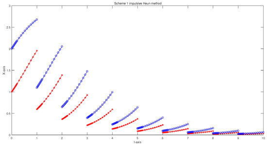
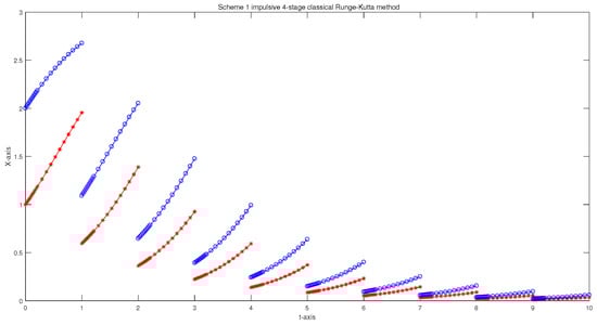
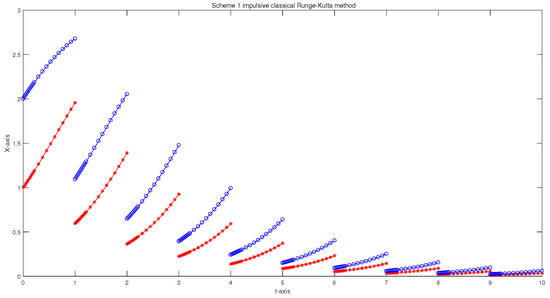
This statement is correct. By Theorems 4 and 8, if the stability function $\mathit{R}\left(z\right)={\displaystyle \frac{P_{\mathit{j}}\left(z\right)}{Q_{\mathit{k}}\left(z\right)}}$ with nonnegative coefficients of S1IRKM (8) (or S2IRKM (21)), then S1IRKM (8) (or S2IRKM (21)) for (50) is asymptotically stable if $\mathit{k}$ is even and the step sizes are small enough. For example, the scheme 1 impulsive Heun’s method (S1IHM) (see Figure 1) and scheme 1 impulsive four-stage four-order classical Runge–Kutta method (S1IRKM) (see Figure 2) for (50) is asymptotically stable.

Figure 1. The S1IHM for DEDI (50) with initial values $x_0=1$ and $y_0=2$, respectively.

Figure 2. The S1IRKM with corresponding classical 4-stage 4-order Runge–Kutta method for DEDI (50) with intitial values $x_0=1$ and $y_0=2$, respectively.

When $x_0=1$, solving (50), we can obtain

$$\begin{array}{cc}\hfill & x\left(t\right)=arccos\left({\displaystyle \frac{C_0{\mathrm{e}}^{-2t}-1}{C_0{\mathrm{e}}^{-2t}+1}}\right),t\in (0,1),\hfill \\ \hfill & x\left(1\right)=\left({\displaystyle \frac{1}{2}}\right)x\left({(1-{\displaystyle \frac{\pi }{4}})}^{-}\right)=\left({\displaystyle \frac{1}{2}}\right)arccos\left({\displaystyle \frac{C_0{\mathrm{e}}^{-2\left(1-\frac{\pi }{4}\right)}-1}{C_0{\mathrm{e}}^{-2\left(1-\frac{\pi }{4}\right)}+1}}\right),\hfill \\ \hfill & x\left(t\right)=arccos\left({\displaystyle \frac{C_1{\mathrm{e}}^{-2t}-1}{C_1{\mathrm{e}}^{-2t}+1}}\right),t\in (1,2),\hfill \\ \hfill & x\left(2\right)=\left({\displaystyle \frac{1}{2}}\right)x\left({(2-{\displaystyle \frac{\pi }{4}})}^{-}\right)=\left({\displaystyle \frac{1}{2}}\right)arccos\left({\displaystyle \frac{C_1{\mathrm{e}}^{-2\left(2-\frac{\pi }{4}\right)}-1}{C_1{\mathrm{e}}^{-2\left(2-\frac{\pi }{4}\right)}+1}}\right),\hfill \\ \hfill & x\left(t\right)=arccos\left({\displaystyle \frac{C_2{\mathrm{e}}^{-2t}-1}{C_2{\mathrm{e}}^{-2t}+1}}\right),t\in (2,3),\hfill \\ \hfill & x\left(3\right)=\left({\displaystyle \frac{1}{2}}\right)x\left({(3-{\displaystyle \frac{\pi }{4}})}^{-}\right)=\left({\displaystyle \frac{1}{2}}\right)arccos\left({\displaystyle \frac{C_2{\mathrm{e}}^{-2\left(3-\frac{\pi }{4}\right)}-1}{C_2{\mathrm{e}}^{-2\left(3-\frac{\pi }{4}\right)}+1}}\right),\hfill \\ \hfill & ⋮\hfill \end{array}$$

where

$$\begin{array}{cc}\hfill & C_0={\displaystyle \frac{1+cos1}{1-cos1}},\hfill \\ \hfill & C_1={\mathrm{e}}^2\left({\displaystyle \frac{1+cos\left[\left(\frac{1}{2}\right)arccos\left(\frac{C_0{\mathrm{e}}^{-2\left(1-\frac{\pi }{4}\right)}-1}{C_0{\mathrm{e}}^{-2\left(1-\frac{\pi }{4}\right)}+1}\right)\right]}{1-cos\left[\left(\frac{1}{2}\right)arccos\left(\frac{C_0{\mathrm{e}}^{-2\left(1-\frac{\pi }{4}\right)}-1}{C_0{\mathrm{e}}^{-2\left(1-\frac{\pi }{4}\right)}+1}\right)\right]}}\right),\hfill \\ \hfill & C_2={\mathrm{e}}^4\left({\displaystyle \frac{1+cos\left[\left(\frac{1}{2}\right)arccos\left(\frac{C_1{\mathrm{e}}^{-2\left(2-\frac{\pi }{4}\right)}-1}{C_1{\mathrm{e}}^{-2\left(2-\frac{\pi }{4}\right)}+1}\right)\right]}{1-cos\left[\left(\frac{1}{2}\right)arccos\left(\frac{C_1{\mathrm{e}}^{-2\left(2-\frac{\pi }{4}\right)}-1}{C_1{\mathrm{e}}^{-2\left(2-\frac{\pi }{4}\right)}+1}\right)\right]}}\right).\hfill \end{array}$$

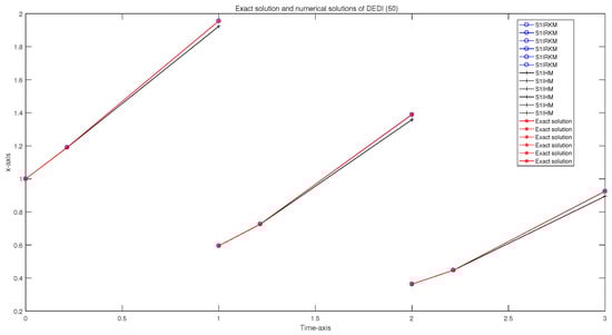
From the theory in the previous part of this paper, we can see that the numerical solutions obtained by scheme 1 impulsive discrete Runge–Kutta methods (See Section 3) converge best. From Table 1, Table 2, Table 3 and Table 4, we can also see that the scheme 1 impulsive discrete Runge–Kutta methods have the best convergence when we use computational simulation, even when the step sizes are not precise enough to have truncation errors. From Figure 3, we can see that the curves of the exact solution of DEDI (50) seem to overlap with those obtained by the S1IRKM and the difference between the curves of the exact solution and those obtained by the S1IHM is not very large. Even if we take the maximum step sizes ${\overline{h}}_{k,1}=1-{\displaystyle \frac{\pi }{4}}$ and ${\overline{h}}_{k,2}={\displaystyle \frac{\pi }{4}}$, $k\in \mathbb{N}$ ($m=1$), the scheme 1 impulsive discrete Runge–Kutta methods are simulated very well.

Table 1. The errors between the numerical solutions obtained from different impulsive schemes with corresponding Heun’s method for (50) and the exact solution of (50) at $t=3$.

	S1IHM		S2IHM		ICHM
$\mathit{m}$	AE	RE	AE	RE	AE	RE
10	7.553082 × 10−6	3.375092 × 10−5	0.008562	0.038261	9.937190 × 10−5	4.440430 × 10−4
20	1.902566 × 10−6	8.501609 × 10−6	0.008458	0.037796	6.538494 × 10−5	2.921723 × 10−4
40	4.774370 × 10−7	2.133426 × 10−6	0.008431	0.037674	2.077670 × 10−5	9.284060 × 10−5
80	1.195843 × 10−7	5.343618 × 10−7	0.001232	0.005504	1.88584928 × 10−6	8.426910 × 10−6
Ratio	3.982459	3.982459	2.953555	2.953555	5.227996	5.227996

Table 2. The errors between the numerical solutions obtained from different impulsive schemes with corresponding classical 4-stage 4-order Runge–Kutta method for (50) and the exact solution of (50) at $t=3$.

	S1IRKM		S2IRKM		ICCRKM
$\mathit{m}$	AE	RE	AE	RE	AE	RE
10	1.626758 × 10−10	7.269161 × 10−10	0.008422	0.037633	3.287970 × 10−7	1.469228 × 10−6
20	1.022230 × 10−11	4.567829 × 10−11	0.008422	0.037633	4.455852 × 10−8	1.991096 × 10−7
40	6.374623 × 10−13	2.848498 × 10−12	0.008422	0.037633	1.003505 × 10−9	4.484159 × 10−9
80	3.674838 × 10−14	1.642100 × 10−13	0.001229	0.005492	5.924100 × 10−10	2.647182 × 10−9
Ratio	16.432140	16.432140	2.950583	2.950583	17.825269	17.825269

Table 3. The errors between the numerical solutions obtained from different impulsive schemes with corresponding Heun’s method for (51) and the exact solution of (51) at $t=3$.

	S1IHM		S2IHM		ICHM
m	AE	RE	AE	RE	AE	RE
10	1.818238 × 10−5	1.806009 × 10−4	0.009707	0.096421	1.826220 × 10−4	0.001814
20	4.602998 × 10−6	4.572040 × 10−5	0.009614	0.095489	4.296101 × 10−5	4.267208 × 10−4
40	1.157979 × 10−6	1.150191 × 10−5	0.002496	0.024787	1.073603 × 10−5	1.066382 × 10−4
80	2.904017 × 10−7	2.884486 × 10−6	0.002488	0.024715	2.638715 × 10−6	2.620969 × 10−5
Ratio	3.970884	3.970884	1.955017	1.955017	4.107037	4.107037

Table 4. The errors between the numerical solutions obtained from different impulsive schemes with corresponding classical 4-stage 4-order Runge–Kutta method for (51) and the exact solution of (51) at $t=3$.

	S1IRKM		S2IRKM		ICCRKM
$\mathit{m}$	AE	RE	AE	RE	AE	RE
10	1.007330 × 10−9	1.000556 × 10−8	0.009581	0.095163	2.293592 × 10−6	2.278166 × 10−5
20	6.376583 × 10−11	6.333697 × 10−10	0.009581	0.095163	2.057541 × 10−7	2.043703 × 10−6
40	3.940667 × 10−12	3.914164 × 10−11	0.002486	0.0246901	3.088753 × 10−8	3.067981 × 10−7
80	1.746658 × 10−13	1.734911 × 10−12	0.002486	0.0246901	3.531197 × 10−9	3.507448 × 10−8
Ratio	18.180002	18.180002	1.9514301	1.9514301	8.851896	8.851896

Figure 3. The exact solution of DEDI (50) and the numerical solutions obtained from S1IRKM and S1IHM for DEDI (50), respectively, when the initial values $x_0=1$.

Example 2. 

The above theory also holds for the following linear DEDI:

$$\left\{\begin{array}{cc}{x}^{\prime }\left(t\right)=x\left(t\right),\hfill & t\ge 0,t\ne k,k=1,2,\cdots ,\hfill \\ x\left(k\right)=\left({\displaystyle \frac{1}{3}}\right)x\left({(k-{\displaystyle \frac{2}{3}})}^{-}\right),\hfill & k\in {\mathbb{Z}}^{+},\hfill \\ x\left(0\right)=x_0.\hfill \end{array}\right.$$

(51)

Applying mathematical induction, the exact solution to DEDI (51) can be obtained by direct calculation as follows, for $k\in \mathbb{N}$,

$$x\left(t\right)=x_0{\left({\displaystyle \frac{1}{3}}{\mathrm{e}}^{{\displaystyle \frac{1}{3}}}\right)}^k{\mathrm{e}}^{t-k},t\in [k,k+1).$$

Obviously, $\alpha =1$, $\sigma ={\displaystyle \frac{1}{3}}$, ${\tau }_k=k$, ${\beta }_k={\displaystyle \frac{1}{3}}$, $k\in {\mathbb{Z}}^{+}$. So

$${\beta }_k{\mathrm{e}}^{\alpha \sigma ({\tau }_k-{\tau }_{k-1})}=\left({\displaystyle \frac{1}{3}}\right){\mathrm{e}}^{\left({\displaystyle \frac{1}{3}}\right)(k-(k-1))}={\displaystyle \frac{{\mathrm{e}}^{\frac{1}{3}}}{3}}<1.$$

Therefore, by Theorem 1, the exact solution of (51) is asymptotically stable.

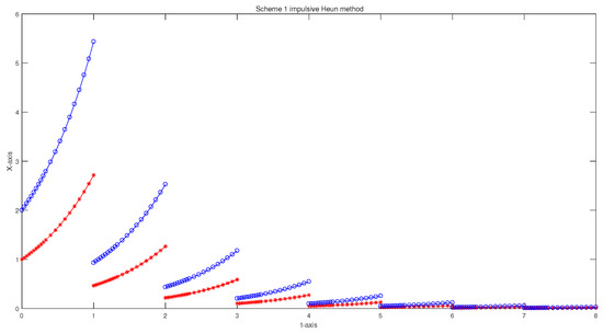
By Theorems 4 and 8, if the stability function $\mathit{R}\left(z\right)={\displaystyle \frac{P_{\mathit{j}}\left(z\right)}{Q_{\mathit{k}}\left(z\right)}}$ with nonnegative coefficients of S1IRKM (8) (or S2IRKM (21)), then S1IRKM (8) (or S2IRKM (21)) for (51) is asymptotically stable if $\mathit{k}$ is even and the step sizes are small enough. For example, the S1IHM (see Figure 4) and S1IRKM (see Figure 5) for (51) is asymptotically stable.

Figure 4. The S1IHM for DEDI (51) with initial values $x_0=1$ and $y_0=2$, respectively.

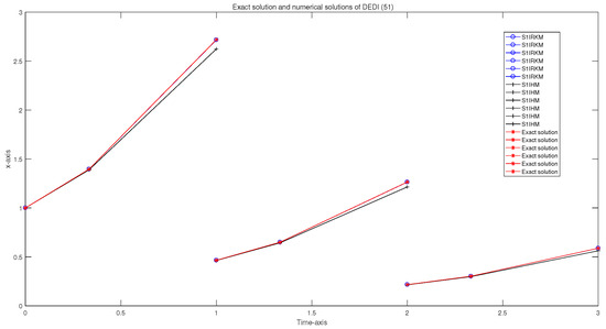
Figure 5. The S1IRKM for DEDI (51) with initial values $x_0=1$ and $y_0=2$, respectively.

Even if we take the maximum step sizes ${\overline{h}}_{k,1}={\displaystyle \frac{2}{3}}$ and ${\overline{h}}_{k,2}={\displaystyle \frac{1}{3}}$, $k\in \mathbb{N}$, ($m=1$), the scheme 1 impulsive discrete Runge–Kutta methods (See Section 3) are simulated very well. From Figure 6, we can see that the curves of the exact solution of DEDI (51) seem to overlap with those obtained by the S1IRKM and the difference between the curves of the exact solution and those obtained by the S1IHM is not very large.

Figure 6. The exact solution of DEDI (51) and the numerical solutions obtained from S1IRKM and S1IHM for DEDI (51), respectively, when the initial values $x_0=1$.

Consider the following impulsive continuous Heun’s method (ICHM) with corresponding two-stage Heun’s method of order $p=2$, interpolated by its unique natural continuous extension of order $q=1$.

From Theorem 3, S1IHM for DEDIs (1), (50) and (51) is convergent of order 2. From Theorem 7, S2IHM for DEDIs (1), (50) and (51) is convergent at least of order 1. Applying Theorem 11, we know that the above ICHM for DEDIs (1), (50) and (51) is convergent of order $q^{\prime }=2$. These results are in general agreement with those obtained from the numerical experiments in Table 1 and Table 3.

Similarly, consider the following impulsive continuous classical Runge–Kutta method (ICCRKM) with corresponding four-stage classical Runge–Kutta method of order $p=4$, interpolated by its unique natural continuous extension of order $q=2$.

From Theorem 3, S1IRKM with corresponding classical four-stage four-order Runge–Kutta method for DEDIs (1), (50) and (51) is convergent of order 4. From Theorem 7, S2IRKM for DEDIs (1), (50) and (51) is convergent at least of order 1. Applying Theorem 11, we know that the above ICCRKM for DEDIs (1), (50) and (51) is convergent of order $q^{\prime }=3$. These results are in general agreement with those obtained from the numerical experiments in Table 2 and Table 4.

AE denotes the absolute errors between the numerical solutions and the exact solutions of DEDIs in Table 1, Table 2, Table 3 and Table 4. Similarly, RE denotes the relative errors between the numerical solutions and the exact solutions of DEDIs.

As can be seen from Table 1 and Table 3, when the step size is halved, both AE and RE of the scheme 1 impulsive Heun’s method (S1IHM) and impulsive continuous Heun’s method ((ICHM)) for DEDIs (50) and (51) become one-quarter of the original ones, respectively, which roughly indicates that both the S1IHM and ICHM for DEDIs (50) and (51) are convergent of order 2. On the other hand, when the step size is halved, both AE and RE of the scheme 2 impulsive Heun’s method (S2IHM) for DEDIs (50) and (51) become one half of the original ones, respectively, which roughly indicates that both the S2IHM for DEDIs (50) and (51) are convergent of order 1.

As can be seen from Table 2 and Table 4, when the step size is halved, both AE and RE of the scheme 1 impulsive classical four-stage four-order Runge–Kutta method (S1IRKM) for DEDIs (50) and (51) become one-sixteenth of the original ones, which roughly indicates that the S1ICRKM for DEDIs (50) and (51) is convergent of order 4. On the other hand, when the step size is halved, both AE and RE of the scheme 2 impulsive classical four-stage four-order Runge–Kutta method (S2IRKM)for DEDIs (50) and (51) become half of the original ones, which roughly indicates that the S2IRKM for DEDIs (50) and (51) is convergent of order 1.

As can be seen from Table 4, when the step size is halved, both AE and RE of ICCRKM for DEDI (51) become one-eighth of the original ones, which roughly indicates that ICRKM for DEDI (51) is convergent of order 3. However, in Table 2, the magnitude of the ratios of AE and RE of ICCRKM for DEDI (50) vary a little bit, but the overall look of convergence is faster than one-eighth.

7. Conclusions and Future Works

The first innovation of this paper is to consider nonlinear Lipschitz continuous function $f(t,x)$ for the dynamic system and for the impulsive term a Lipschitz continuous function $I_k$, which also implies new sufficient conditions for asymptotical stability of the exact solutions, and numerical solutions of DEDIs are obtained. Another innovation of this paper is that different numerical methods are constructed in order to obtain efficient numerical formats for higher-order convergence, as follows. (1) The simplest and most straightforward idea is to select the times at discontinuous points ${\tau }_k$, (the moments of impulsive effects) $k\in {\mathbb{Z}}^{+}$ and the past times $r_k$ involved in calculating the exact (or numerical) solution of the discontinuities as step nodes of the numerical method, which is also the numerical method (S1RKM) with the best convergence. The S1IRKMs are convergent of order p if the corresponding Runge–Kutta method is p-order. (2) The second idea is to select only the discontinuities ${\tau }_k$ as step nodes and instead of the past times $r_k$ being selected as step nodes for the numerical method, the times $t_{k,\lfloor \sigma m\rfloor }$ near the past times $r_k$ are taken and selected as step nodes, which is the main idea behind the construction of S2RKM. The S2IRKMs for DEDI (1) in the general case are only convergent of order 1, but are more efficient and may be suitable for more complex DEDIs. Thus in this case, we only need to use the S2$\theta$M, which is also convergent of order 1 and simpler. (3) When the past times $r_k$ are not chosen as step nodes, in order to overcome the convergence order problem that occurs, in the second idea, we can use the ICRKM. In this article, we prove that ICRKM for DEDI (1) is convergent of order $q^{\prime }=min\{p,q\}$, if the corresponding continuous Runge–Kutta method is consistent of order p and is consistent of uniform order q.

When the past times $r_k$ involved in DEDIs at the moments of impulsive effects are state-dependent or stochastic, it is difficult or impossible for the past moments to be taken as step nodes, which is a problem we will address in the future. In other words, applying S2I$\theta$Ms or ICRKMs to solve time-delay differential equations with state-dependent delayed impulses or differential equations with stochastic delayed impulses will be the future work. What happens if the function $I_k$ in an impulsive term is not a continuous Lipschitz function? This is also a question we will study in the future.

References

- Bainov, D.D.; Simeonov, P.S. Systems with Impulsive Effect: Stability, Theory and Applications; Ellis Horwood: Chichester, UK, 1989. [Google Scholar]
- Bainov, D.D.; Simeonov, P.S. Impulsive Differential Equations: Asymptotic Properties of the Solutions; World Scientific: Singapore, 1995. [Google Scholar]
- Lakshmikantham, V.; Bainov, D.D.; Simeonov, P.S. Theory of Impulsive Differential Equations; World Scientific: Singapore, 1989. [Google Scholar]
- Samoilenko, A.M.; Perestyuk, N.A.; Chapovsky, Y. Impulsive Differential Equations; World Scientific: Singapore, 1995. [Google Scholar]
- Li, X.D.; Song, S.J. Impulsive Systems with Delays: Stability and Control; Science Press: Beijing, China, 2022. [Google Scholar]
- Li, X.D.; Song, S.J.; Wu, J.H. Exponential stability of nonlinear systems with delayed impulses and applications. IEEE Trans. Automat. Control 2019, 64, 4024–4034. [Google Scholar] [CrossRef]
- Yu, Z.Q.; Ling, S.; Liu, P.X. Exponential stability of time-delay systems with flexible delayed impulse. Asian J. Control. 2024, 26, 265–279. [Google Scholar] [CrossRef]
- Jiang, B.; Lu, J.; Liu, Y. Exponential stability of delayed systems with average-delay impulses. SIAM J. Control Optim. 2020, 58, 3763–3784. [Google Scholar] [CrossRef]
- He, Z.L.; Li, C.D.; Cao, Z.R.; Li, H.F. Stability of nonlinear variable-time impulsive differential systems with delayed impulses. Nonlinear Anal. Hybrid Syst. 2021, 39, 100970. [Google Scholar] [CrossRef]
- Lu, Y.; Zhu, Q.X. Exponential stability of impulsive random delayed nonlinear systems with average-delay impulses. J. Frankl. Inst. 2024, 361, 106813. [Google Scholar] [CrossRef]
- Chen, X.Y.; Liu, Y.; Ruan, Q.H.; Cao, J.D. Stabilization of nonlinear time-delay systems: Flexible delayed impulsive control. Appl. Math. Model. 2023, 114, 488–501. [Google Scholar] [CrossRef]
- Chen, W.H.; Zheng, W.X. Exponential stability of nonlinear time-delay systems with delayed impulse effects. Automatica 2011, 47, 1075–1083. [Google Scholar] [CrossRef]
- Cui, Q.; Li, L.L.; Cao, J.D. Stability of inertial delayed neural networks with stochastic delayed impulses via matrix measure method. Neurocomputing 2022, 471, 70–78. [Google Scholar] [CrossRef]
- Li, X.D.; Zhang, X.L.; Song, S.J. Effect of delayed impulses on input-to-state stability of nonlinear systems. Automatica 2017, 76, 378–382. [Google Scholar] [CrossRef]
- Liu, W.L.; Li, P.; Li, X.D. Impulsive systems with hybrid delayed impulses: Input-to-state stability. Nonlinear Anal. Hybrid Syst. 2022, 46, 101248. [Google Scholar] [CrossRef]
- Niu, S.N.; Chen, W.H.; Lu, X.M.; Xu, W.X. Integral sliding mode control design for uncertain impulsive systems with delayed impulses. J. Frankl. Inst. 2023, 360, 13537–13573. [Google Scholar] [CrossRef]
- Kuang, D.P.; Li, J.L.; Gao, D.D. Input-to-state stability of stochastic differential systems with hybrid delay-dependent impulses. Commun. Nonlinear Sci. Numer. Simul. 2024, 128, 107661. [Google Scholar] [CrossRef]
- Ran, X.J.; Liu, M.Z.; Zhu, Q.Y. Numerical methods for impulsive differential equation. Math. Comput. Model. 2008, 48, 46–55. [Google Scholar] [CrossRef]
- Liu, X.; Song, M.H.; Liu, M.Z. Linear multistep methods for impulsive differential equations. Discrete Dyn. Nat. Soc. 2012, 2012, 652928. [Google Scholar] [CrossRef]
- Zhang, Z.H.; Liang, H. Collocation methods for impulsive differential equations. Appl. Math. Comput. 2014, 228, 336–348. [Google Scholar] [CrossRef]
- Liu, M.Z.; Liang, H.; Yang, Z.W. Stability of Runge–Kutta methods in the numerical solution of linear impulsive differential equations. Appl. Math. Comput. 2007, 192, 346–357. [Google Scholar] [CrossRef]
- Zhang, G.L. Asymptotical stability of numerical methods for semi-linear impulsive differential equations. Comput. Appl. Math. 2020, 39, 17. [Google Scholar] [CrossRef]
- Liang, H.; Song, M.H.; Liu, M.Z. Stability of the analytic and numerical solutions for impulsive differential equations. Appl. Numer. Math. 2011, 61, 1103–1113. [Google Scholar] [CrossRef]
- Liang, H.; Liu, M.Z.; Song, M.H. Extinction and permanence of the numerical solution of a two-preyone-predator system with impulsive effect. Int. J. Comput. Math. 2011, 88, 1305–1325. [Google Scholar] [CrossRef]
- Liang, H. hp-Legendre-Gauss collocation method for impulsive differential equations. Int. J. Comput. Math. 2015, 94, 151–172. [Google Scholar] [CrossRef]
- Wen, L.P.; Yu, Y.X. The analytic and numerical stability of stiff impulsive differential equations in Banach space. Appl. Math. Lett. 2011, 24, 1751–1757. [Google Scholar] [CrossRef][Green Version]
- Zhang, G.L. Convergence, consistency and zero stability of impulsive one-step numerical methods. Appl. Math. Comput. 2022, 423, 127017. [Google Scholar] [CrossRef]
- Liu, X.; Zhang, G.L.; Liu, M.Z. Analytic and numerical exponential asymptotic stability of nonlinear impulsive differential equations. Appl. Numer. Math. 2014, 81, 40–49. [Google Scholar] [CrossRef]
- Zhang, G.L. Asymptotical stability of Runge–Kutta methods for nonlinear impulsive differential equations. Adv. Differ. Equ. 2020, 2020, 42. [Google Scholar] [CrossRef]
- Ding, X.; Wu, K.N.; Liu, M.Z. The Euler scheme and its convergence for impulsive delay differential equations. Appl. Math. Comput. 2010, 216, 1566–1570. [Google Scholar] [CrossRef]
- Zhang, G.L.; Song, M.H.; Liu, M.Z. Asymptotical stability of the exact solutions and the numerical solutions for a class of impulsive differential equations. Appl. Math. Comput. 2015, 258, 12–21. [Google Scholar] [CrossRef]
- Zhang, G.L.; Song, M.H. Asymptotical stability of Runge–Kutta methods for advanced linear impulsive differential equations with piecewise constant arguments. Appl. Math. Comput. 2015, 259, 831–837. [Google Scholar] [CrossRef]
- Zhang, G.L.; Song, M.H.; Liu, M.Z. Exponential stability of the exact solutions and the numerical solutions for a class of linear impulsive delay differential equations. J. Comput. Appl. Math. 2015, 285, 32–44. [Google Scholar] [CrossRef]
- Zhang, G.L. High order Runge–Kutta methods for impulsive delay differential equations. Appl. Math. Comput. 2017, 313, 12–23. [Google Scholar] [CrossRef]
- Zhang, G.L.; Song, M.H. Impulsive continuous Runge–Kutta methods for impulsive delay differential equations. Appl. Math. Comput. 2019, 341, 160–173. [Google Scholar] [CrossRef]
- Wu, K.N.; Ding, X. Convergence and stability of Euler method for impulsive stochastic delay differential equations. Appl. Math. Comput. 2014, 229, 151–158. [Google Scholar] [CrossRef]
- Zhang, G.L.; Liu, C. Two schemes of impulsive Runge–Kutta methods for linear differential equations with delayed impulses. Mathematics 2024, 12, 2075. [Google Scholar] [CrossRef]
- Bellen, A. One-step collocation for delay differential equations. J. Comput. Appl. Math. 1984, 183, 275–283. [Google Scholar] [CrossRef]
- Bellen, A.; Zennaro, M. Numerical Methods for Delay Differential Equations; Clarendon Press: Oxford, UK, 2003. [Google Scholar]
- Brunner, H. Collocation Methods for Volterra Integral and Related Functional Differential Equations; Cambridge University Press: Cambridge, UK, 2004. [Google Scholar]
- Brunner, H.; Liang, H. Stability of collocation methods for delay differential equations with vanishing delays. BIT Numer. Math. 2010, 50, 693–711. [Google Scholar] [CrossRef]
- Liang, H.; Brunner, H. Collocation methods for differential equations with piecewise linear delays. Commun. Pure Appl. Anal. 2012, 11, 1839–1857. [Google Scholar] [CrossRef]
- Engelborghs, K.; Luzyanina, T.; Houty, K.J.I.; Roose, D. Collocation methods for the computation of periodic solutions of delay differential equations. SIAM J. Sci. Comput. 2001, 5, 1593–1609. [Google Scholar] [CrossRef]
- Butcher, J.C. Numerical Methods for Ordinary Differential Equations; Wiley: Hoboken, NJ, USA, 2003. [Google Scholar]
- Dekker, K.; Verwer, J.G. Stability of Runge–Kutta Methods for Stiff Nonlinear Differential Equations; North-Holland: Amsterdam, The Netherlands, 1984. [Google Scholar]
- Hairer, E.; Nørsett, S.P.; Wanner, G. Solving Ordinary Differential Equations I; Nonstiff Problems; Springer: New York, NY, USA, 1993. [Google Scholar]
- Hairer, E.; Nørsett, S.P.; Wanner, G. Solving Ordinary Differential Equations II; Stiff Problems; Springer: New York, NY, USA, 1993. [Google Scholar]
- Wanner, G.; Hairer, E.; Nϕrsett, S.P. Order stars and stability theorems. BIT 1978, 18, 475–489. [Google Scholar] [CrossRef]
- Song, M.H.; Yang, Z.W.; Liu, M.Z. Stability of θ-methods for advanced differential equations with piecewise continuous arguments. Comput. Math. Appl. 2005, 49, 1295–1301. [Google Scholar] [CrossRef]
- Wang, Q.; Qiu, S. Oscillation of numerical solution in the Runge–Kutta methods for equation x′(t) = ax(t) + a0x([t]). Acta Math. Appl. Sin. Engl. Ser. 2014, 30, 943–950. [Google Scholar] [CrossRef]
- Yang, Z.W.; Liu, M.Z.; Song, M.H. Stability of Runge–Kutta methods in the numerical solution of equation u′(t) = au(t) + a0u([t]) + a1u([t − 1]). Appl. Math. Comput. 2005, 162, 37–50. [Google Scholar] [CrossRef]
Disclaimer/Publisher’s Note: The statements, opinions and data contained in all publications are solely those of the individual author(s) and contributor(s) and not of MDPI and/or the editor(s). MDPI and/or the editor(s) disclaim responsibility for any injury to people or property resulting from any ideas, methods, instructions or products referred to in the content. |
© 2024 by the authors. Licensee MDPI, Basel, Switzerland. This article is an open access article distributed under the terms and conditions of the Creative Commons Attribution (CC BY) license (https://creativecommons.org/licenses/by/4.0/).