Abstract
Effects of the road, such as speed bumps, can significantly affect a car’s stability. This study focuses on how a quarter-car model is affected by a basic harmonic speed hump and how Cubic Negative Velocity Control (CNVC) is used to control the amplitude of disturbances. This study differs from earlier research in considering various control and force kinds that impact the system. The external forces in this context are a component of a non-linear dynamic system. Two-degree-of-freedom (2DOF) differential coupled equations describe the system’s equation. Numerous numerical experiments have been conducted, including proportional derivative (PD), negative derivative feedback (NDF), positive position feedback (PPF), linear negative velocity control (LNVC), and CNVC; the results show that when the hump is represented as a simple harmonic hump, CNVC has the best effect and can regulate vibrations more precisely than the other approaches on this system. Subsequently, the vibration value of the system was numerically analyzed both before and after the control was implemented. Using the frequency response equation and phase plane approaches in conjunction with the Runge–Kutta fourth order method (RK-4) in the context of resonance situation analysis, the stability of the numerical solution has been evaluated.
Keywords:
suspension system; averaging technique; cubic negative velocity control; speed humps; simple harmonic hump; non-linear dynamical system MSC:
65P40; 70K20; 74H10; 74H45
1. Introduction
Different problems on the road affect the stability of vehicles as speed humps. Humps are raised bands across a road, designed to make drivers reduce their speed, especially in built-up areas, and are just a different solution to the problem of slowing down vehicles. Speed humps tend to be slightly smaller in height than speed bumps but longer, whereas speed bumps are taller and more likely to be found in a parking lot. Speed humps are a great way to calm and control traffic vehicular traffic on your site. They help to focus a driver’s attention in critical areas where additional safety measures are needed. Humps are made from a wide variety of materials, such as concrete, metal, plastic, and tarmac.
Gobbi et al. [1] examined a new strategy for creating automobile suspension systems that integrated the principles of resilient design and multi-objective programming, and developed analytical solutions with an advanced method inspired by the Fritz John necessity condition. Khorshid and Alfares [2] employed a mathematical model to simulate the effects of Speed Control Hump (SCH) geometry on vehicle–human dynamics to enhance its performance. The refinement of the model resulted in a significant improvement in its ability to simulate the actual response.
Amer et al. [3] applied the method of multiple time scale perturbation to address the nonlinear differential equations, while simultaneously mitigating and reducing vibrations within the twin-tail aircraft’s dynamic system through the implementation of two straightforward active control laws rooted in linear negative velocity and acceleration feedback. Dai et al. [4] regarded tire stiffness, suspension damping, sprung mass, and unsprung mass as random variables. Using the functional moment approach for the random variable and the algebraic synthesis technique, they were able to develop and alter the result. El-Ganaini et al. [5] obtained an approximate solution by applying the multiple scales method and adding a positive position feedback (PPF) controller to control vibration. They extracted the perfect acting conditions of the system and proved that all results from analytical solutions are in good agreement with the numerical simulation.
Hassaan [6,7] investigated the dynamics of a quarter-car model when using the novel simple harmonic in part one and the novel polynomial hump in part two. He was able to reach the appropriate measurements for bumps and their heights with vehicle speeds and reach the appropriate results for safer driving and high stability of the vehicles. Huang et al. [8] studied their work that acts on car body-mounted equipment on the car body’s flexible vibration. The main goals were to get the passenger of body flexible vibration and ride comfort. Silveira et al. [9] investigated how asymmetric viscous damping car suspension systems behave under harmonic excitation. They obtained an analytical approximation using harmonic balance. By reducing the effect of the uneven road on the displacement, acceleration, and damping of the sprung mass, the selection of asymmetry ratio eventually enhances comfort. Ghasabi et al. [10] showed that the use of a proportional derivative time delay controller reduces oscillations of a continuous spinning shaft with the use of Routh–Hurwitz criteria obtained for stable and unstable zones of the system.
Using the time-varying nonlinear contact load of an axle box bearing, Li et al. [11] created a spatially coupled dynamic model for the vehicle. The dynamic coupled connection between the wheel and rail was then used to create a spatially coupled dynamic model for the vehicle track, and it proved the ability to effectively reflect the vibration characteristics of locomotives. Azimov and Yakubjanova [12], Azimov et al. [13], and Azimov and Ikhsanova [14] solved the problem of the movement of semi-mounted cotton harvesters on slopes; they compiled the equations of motion of a Cotton Harvester (CH), using the example of the MX-2.4 brand, using the Lagrange equations of the second kind, and solved the equations of vertical oscillations of the machine when driving on slopes numerically using the Runge–Kutta method. Taking into account the uneven distribution in system and the power of the vibration of the machine and the wheels.
Dumitriu [15] studied a time-delayed proportional-derivative (TDPD) controller with quadratic and cubic nonlinearities which had its oscillations reduced and its performance enhanced for potential future uses of the car body able vibrations in a high-speed railway vehicle. Using the average approach, Bauomy and EL-Sayed [16] were able to determine the first-order approximation solutions. Finally, they improved performance and decreased fluctuating maximum peak overshoot. Łuczko and Ferde [17] added an extra inner cylinder with an auxiliary piston to the structure of the traditional monotube hydraulic shock absorber’s structure; the novel idea allowed them to isolate and minimize the vibration of the automobile body to confirm the operational efficacy of the suggested shock absorber, which is susceptible to random and impulse excitations.
Stojanovic et al. [18] discussed the importance of the suspension system in the vehicle to reduce shocks resulting from uneven road and maintain stability in the wheelhouse. Finally, they concluded that the most significant influence on the displacement of the sprung mass is the stiffness of the spring, which results from using MATLAB/SIMULINK software R2023b. Le and Tran [19] investigated the act of a two-stage asymmetric damper on the dynamic responses under transitory road inputs in the range of different vehicle velocities. They found that a two-stage asymmetric damper maintains a better ride comfort level but offers the bus less treatment stability and working space. Zhang et al. [20] obtained results that show that the magneto-rheological (MR) nonlinear response behavior of the half car is mostly concentrated in the medium frequency range for low and mid speeds that are concerned with the ride comfort performance of the vehicle. Wagh [21] designed a conceptual model and all the ingredients required to fix the test rig to the ground. This was done by considering the motion dynamics, then simulating the result, as he was able to fix the in-house Adams software package (developed by Hexagon (https://hexagon.com)) on the test rig to validate the system. Alhelou et al. [22] developed an active suspension control algorithm for the full car model to perfect properties with active disturbance rejection control. The result simulated the effectiveness of an active suspension system with the proposed algorithm to increase holding characteristics on the road. Shi et al. [23] showed in their results that the D-inerter has a broader bandwidth of enhanced isolation and the lower resonant peak is decreased by 21.5% at a speed of 30 m/s, reducing the Root Mean Square (RMS) of vehicle body acceleration.
Kandel et al. [24] concentrated on a mass-damper-spring model and employed a positive position feedback (PPF) controller to regulate vibrations and to obtain an approximate solution using the averaging perturbation method. Kandel et al. [25,26] discussed a model featuring a mass-damper-spring configuration controlled by a Cubic-Position Negative-Velocity Feedback (CPNV) controller. Kandel et al. [27] controlled the mass-damper-spring model via the nonlinear saturation controller (NSC) of the harmonically excited car. Graphical plots in 2D and 3D were provided, which were based on the equations obtained through the harmonic balance method. Kandel and Hamed [28] applied the multiple scales perturbation technique to derive an approximate solution for a horizontally supported car model. By incorporating an integral resonant controller (IRC), they successfully regulated the vibrations of this system.
The findings of Darus and Enzai [29] indicated that the Linear Quadratic Regulator (LQR) control strategy has a drawback. Compared to Proportional Integral Derivative (PID), it cannot provide good vehicle handling. Compared to LQR, PID is likewise unable to provide superior ride comfort. By increasing the number of iterations in the Particle Swarm Optimization (PSO) algorithm to find the optimal position for the centres of mass of force (MSF), Al-Mutar and Abdalla [30] observed that the displacement of the sprung mass has been reduced by approximately 96.53%, which shows a good improvement in ride comfort and sprung mass and good handling. The fuzzy logic controller (FLC) was designed by PSO for the quarter car active suspension system model to improve a more comfortable ride compared with the passive model.
Altıno [31] discovered that the Cultural Algorithm (CA) performs the best. The primary cause is the other algorithms’ local optimum issue with this situation. Additionally, the PID tuning algorithm can successfully use scalarization techniques to turn a multi-objective problem into a single-objective one. Basargan et al. [32] discovered that for specific road segments and vehicle velocities, a designated comfort-orientated velocity and the matching schedule variable had been specified. Abut and Salkim [33] suggested the control approach (fuzzy-LQR) outperforms the research in the literature by approximately 84.2% of bodies according to their findings.
The novel strategy, sometimes referred to as “a Cubic Negative Velocity Control,” or “CNVC,” lessens the damaging vibration of a quarter-car model in a shorter amount of time and with greater computing efficiency than other controllers. It is also effective in a larger class of non-linear vibrating situations. It also increases the stability of the system. Each of the aforementioned is proved in detail with the results that were obtained. The main objective of this research paper is to analyze, study, and solve the problems of road deformation on vehicles, which makes them unstable, unsafe, and more prone to accidents. Therefore, we studied two different types of road deformations and compared them. We also studied the worst form of vehicle damage. Using Cubic Negative Velocity Control and the averaging method, we can finally manage the vibration issue on the quarter-vehicle model and provide an approximate solution. The MATLAB tool has been utilized to conduct a numerical examination of the effects of different parameters on the performance of the model. In future work, it is possible to work on the text of the vehicle and the effect of deformations on the vehicle body and passengers from the inside to make vehicles more stable on the road.
2. Mathematical Modeling
In vehicle dynamics, the quarter-car model is a condensed representation that is used to examine how a car’s suspension system behaves. One tire, one suspension spring, one suspension damper, and one-fourth of the vehicle’s mass make up the four essential parts of the vehicle. The equation of motion explains how variations in the vertical motion of the road surface affect the sprung mass, which represents the vehicle body. For the quarter-car model, the equations of motion in Ref. [6] are as follows:
where
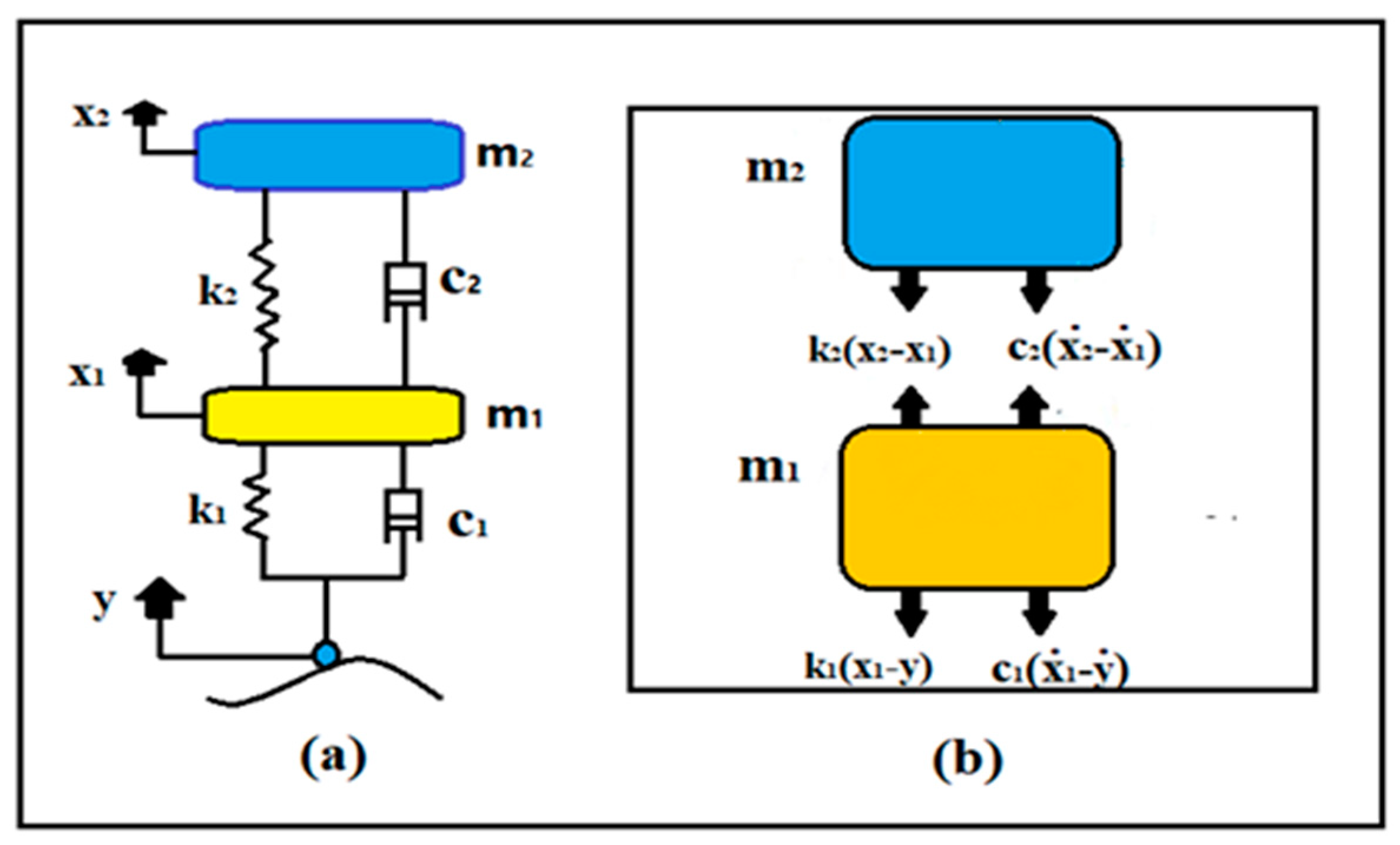
Figure 1 explains the mathematical model of a non-linear dynamical system consisting of 2-DOF differential coupled equations and the system’s equation: (a) the described quarter car system, where there are two bodies: sprung (car) which represents the displacement of the car body, and Unsprang (suspension, wheel, tire) mass which represents the displacement of the wheel. Although it is a simplified model, stiffness and damping of the systems are used so as not to consider everything rigid and the simple harmonic hump. (b) explains the types of forces that affect the system, which are the spring force and the damper force, as in Ref. [7].

Figure 1.
(a) Quarter-car physical model; (b) modeling of the system (force diagram of mass elements).
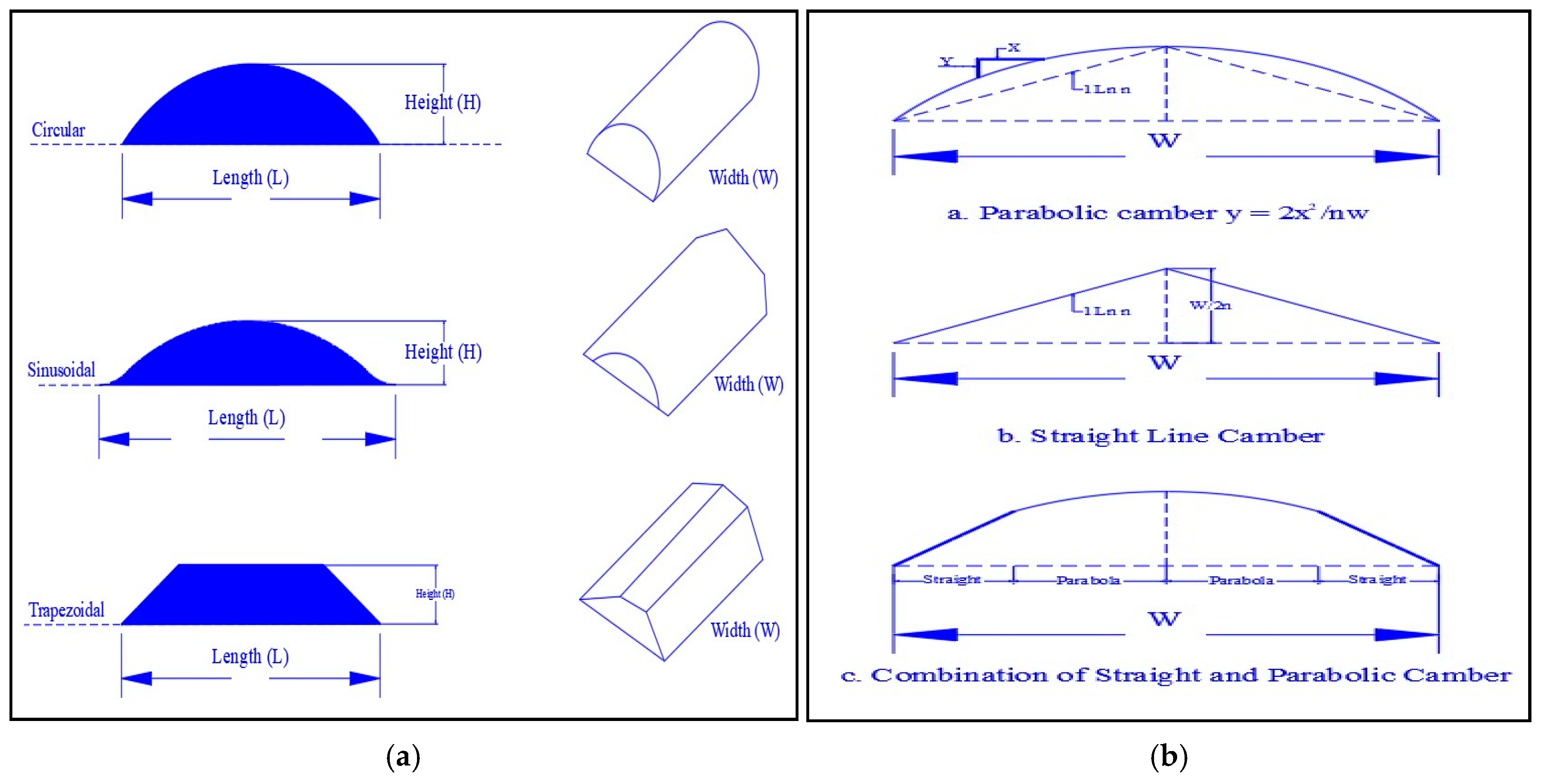
Figure 2a,b depict different types of speed humps commonly found on roads. These speed humps are designed with specific conditions to address various traffic concerns, and each type of speed hump has unique camber, which refers to the curvature of the surface provided to the road or any other paved surface. Understanding the various shapes of speed humps is crucial because different forms can affect the way cars interact with them, potentially causing problems and damage to car bodies and tires.

Figure 2.
(a) Types of road humps; (b) types of camber of road.
3. Equations of Motion with Control
For the quarter-car model, the equations of motion after adding the ideal control are as follows:
These formulas explain how the forces operating on the car, including those from speed bumps, affect the sprung mass’s motion and, in turn, the ride and handling qualities of the car. The answers to these equations in the control case show how the suspension system should be built to minimize vibration and maximize performance, comfort, and stability.
4. Mathematical Analysis
4.1. Mathematical Analysis (Averaging Method)
This section employs the averaging method to determine an approximate solution. Applying Equations (3) and (4), the approximate solution of the first order by using the proposed control (Cubic Negative Velocity Control) method outlined in the Equations controlled system can be obtained by solving the averaging method analytically. The required solution of these equations is written as follows:
where and (n = 1, 2) are constant, Differentiating Equations (5) and (6) concerning yields:
where (n = 1, 2) are constant
and are unknown functions of time t in Equations (3) and (4). Then, differentiating Equations (5) and (6) concerning and comparing with Equations (7) and (8), we get:
Differentiating Equations (7) and (8) once concerning , we get:
Substituting Equations (5)–(8), (11) and (12) into Equations (3) and (4), we obtain:
Then, we get:
4.2. Periodic Solutions
The averaging equations correspond to a numerical analysis; every potential resonance case is examined. In order to investigate the stability of the system, a numerical check was performed to identify the worst resonance cases. Resonance cases that have been chosen are:
where the detuning parameter .
Using only the constant portions and slowly moving parts in Equations (9), (10) and (19) in Equations (13) and (14), we can be introduce the following equations:
where and we have:
4.3. Frequency Response Equations
The stable solutions are examined for the framework’s stability. and the fixed points’ periodic solution in Equations (24)–(27), which led to the following equations being derived from the frequency response equations shown as follows:
where and .
Solving the above nonlinear algebraic equations numerically with the FSOLVE code of MATLAB, we get the frequency response equations within the fixed solutions.
4.4. Stability Solution
The non-linear solution of the obtained fixed points should be examined for stability. Let
where and are solutions of (24)–(27) and are perturbations which are assumed to be small in comparison with and .
Substituting Equation (32) into Equations (24)–(27), preserving the linear terms, then using the trigonometric function and preserving only the linear terms of in Equations (24)–(27), we get the following system of first-order differential equations the following equations are obtained:
Equations (33)–(36) can be presented in the following matrix form:
where is the Jacobian matrix and defined in the Appendix A.
The stability of a given fixed point to a disturbance proportional to exp(λt) is determined by the roots of:
Consequently, a non-trivial solution is stable if and only if the real parts of both eigenvalues of the coefficient matrix Equation (38) are less than zero, which of the following polynomials has the following roots:
where are the coefficients of Equation (40). The Routh–Hurwitz criterion must be satisfied for the aforementioned system’s solution to be stable:
5. Results and Discussion
By applying the Rung–Kutta fourth-order method and keeping a focus on the system’s behavior, showing that study of amplitude on the main system and choosing the worst cases and without absorber, it is also shown that these are the worst resonance cases, such that the oscillations of the system and absorber dynamic chaos are the conditions that must be controlled, using the control to fade the vibration and pressure damage.
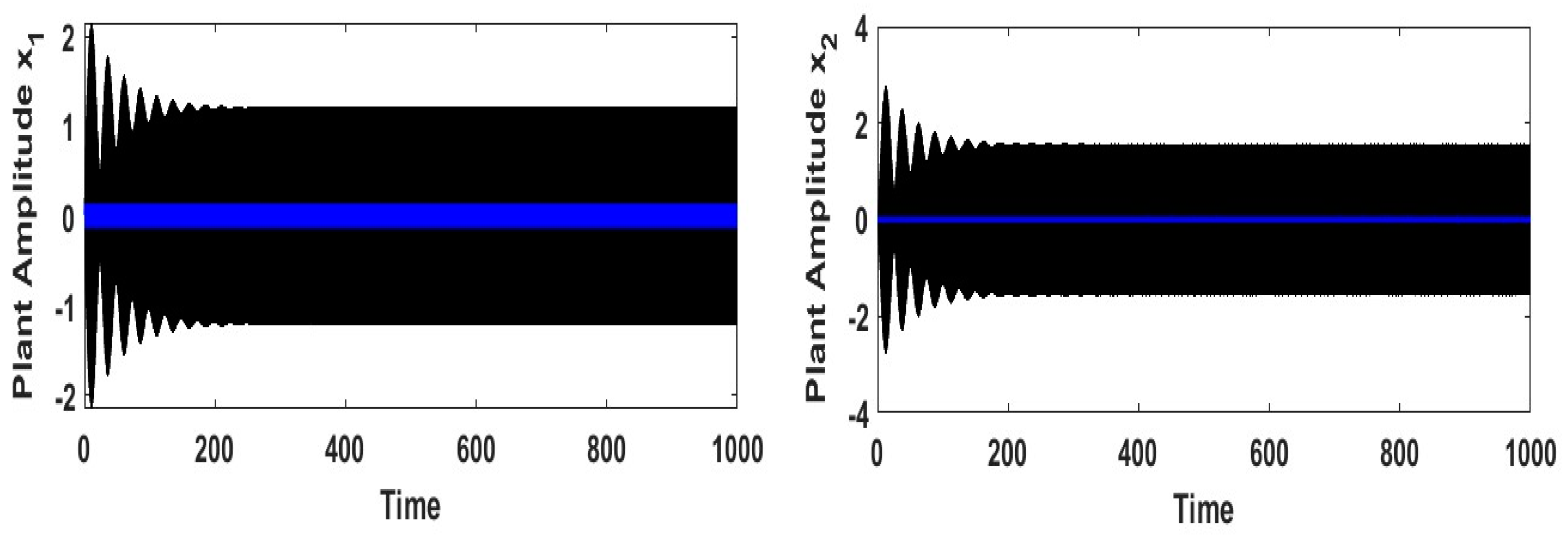
Figure 3 shows the amplitude values after and before CNVC, and we found CNVC to be the most effective, as shown in Figure 3, since it was able to manage and minimize the vibration as much as it could at the rate of 2556%, as shown in Table 1.

Figure 3.
Response of the system at the worst case (black color) and the effectiveness of the best control (CNVC) (blue color).

Table 1.
The values of absolute error and percentage error.
5.1. Frequency Response Curve
Numerical techniques are used to graphically display the frequency equation. Nonlinear algebraic equations, such as the frequency response problem, can be solved quantitatively using the Newton–Raphson technique. The frequency response, Equations (27)–(31), are nonlinear algebraic equations, and the steady-state amplitudes of the frequency response curve against parameter and frequency response curve against parameter resonance , and are displayed in Figure 4, Figure 5, Figure 6, Figure 7 and Figure 8. Then, study of the change effects of parameter values shows that the period of stability and instability changes with the different values of parameters, and the same goes for frequency values.
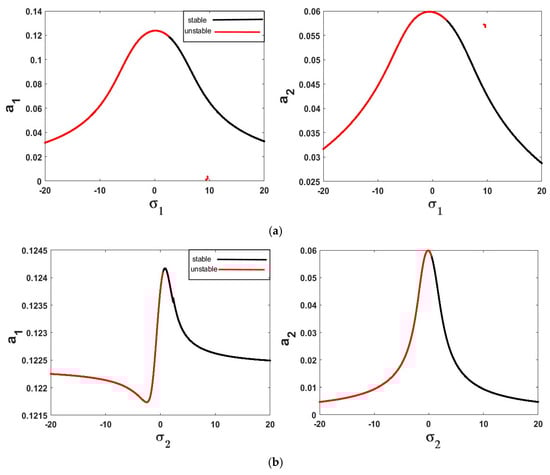
Figure 4.
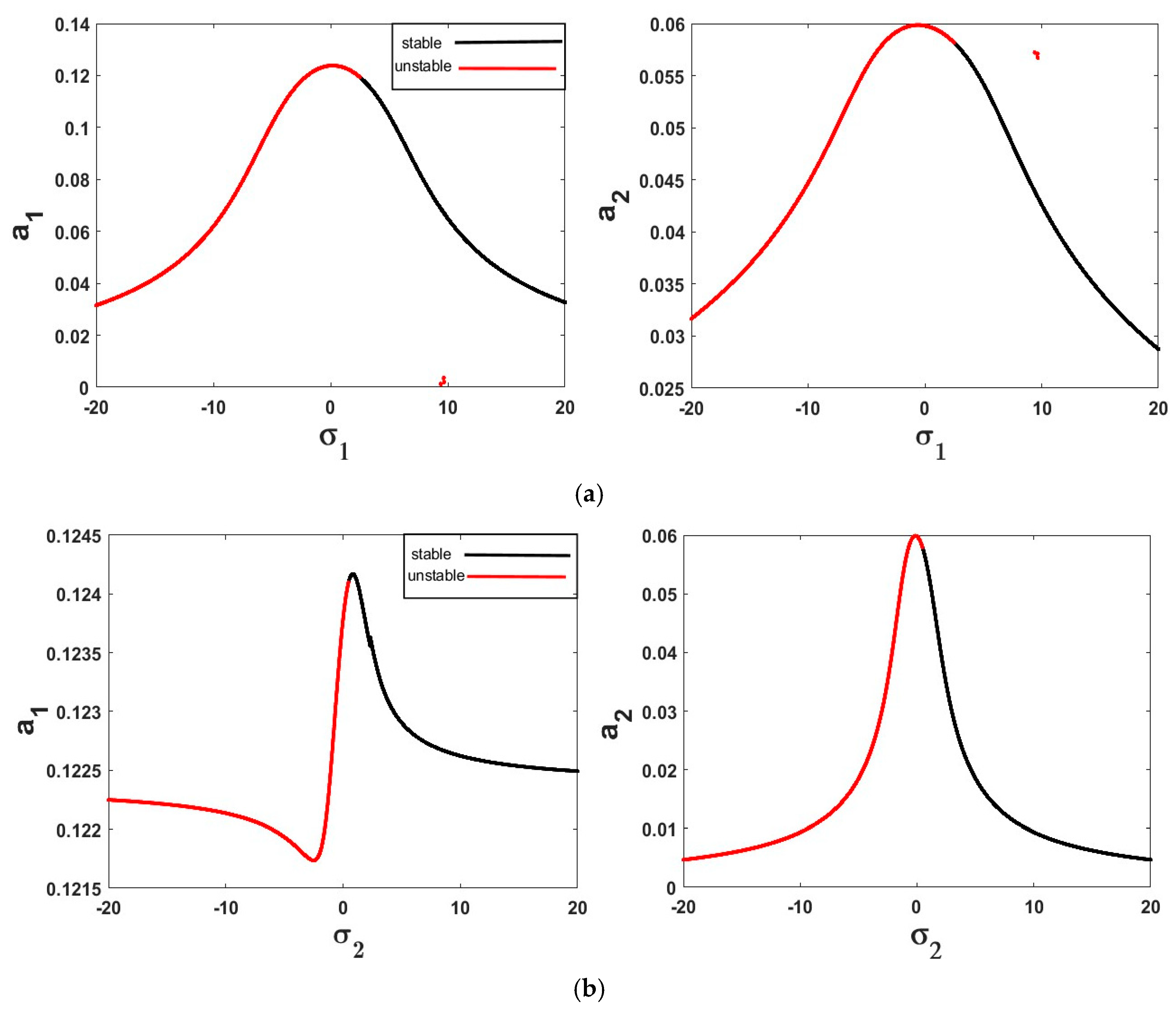
Frequency response curves: (a) stability of the steady-state amplitude ( against ); (b) stability of the steady-state amplitude ( against ).

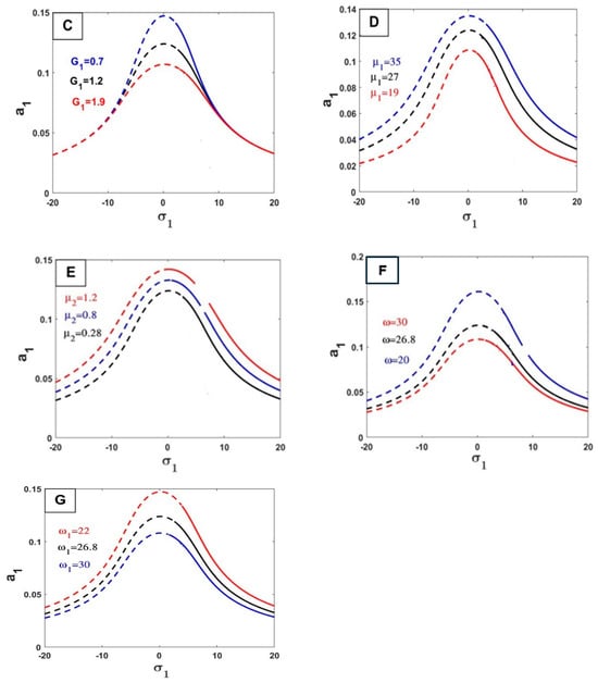
Figure 5.
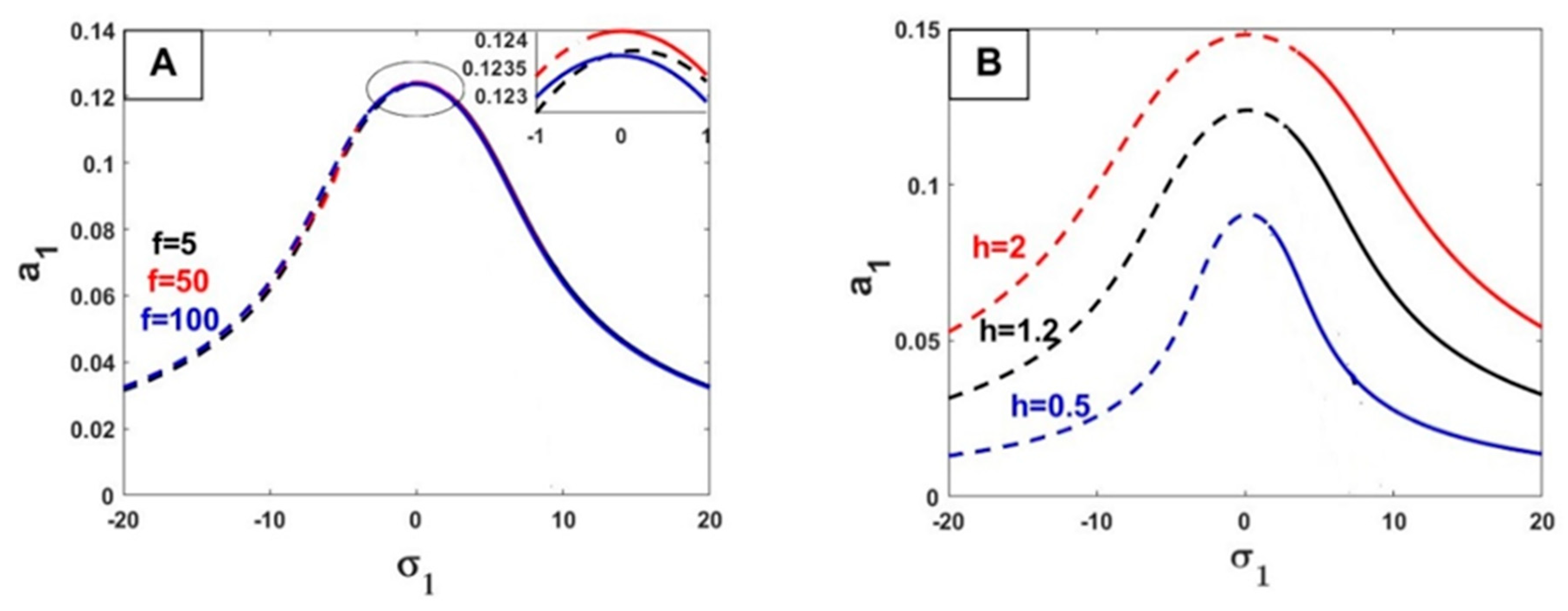
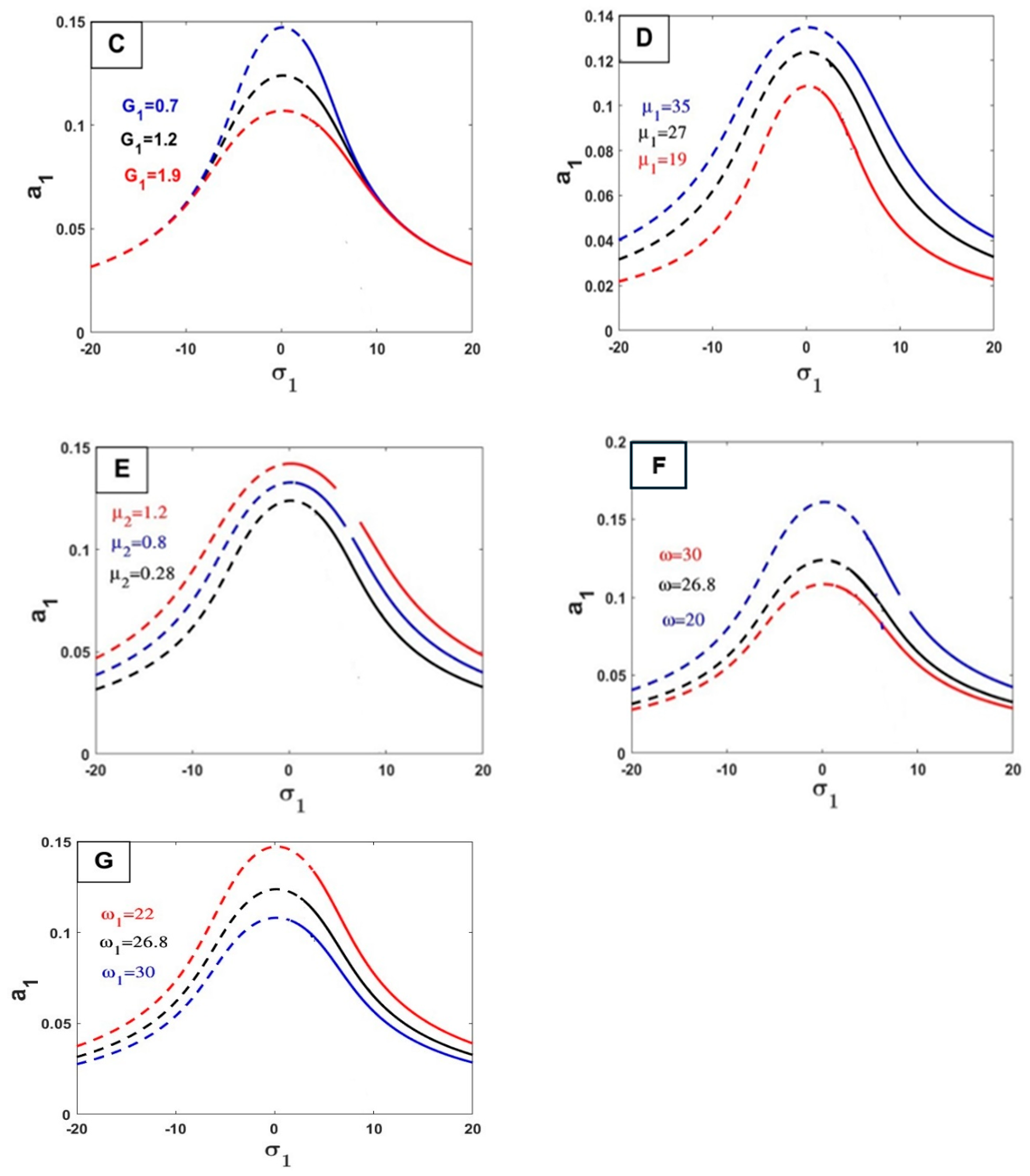
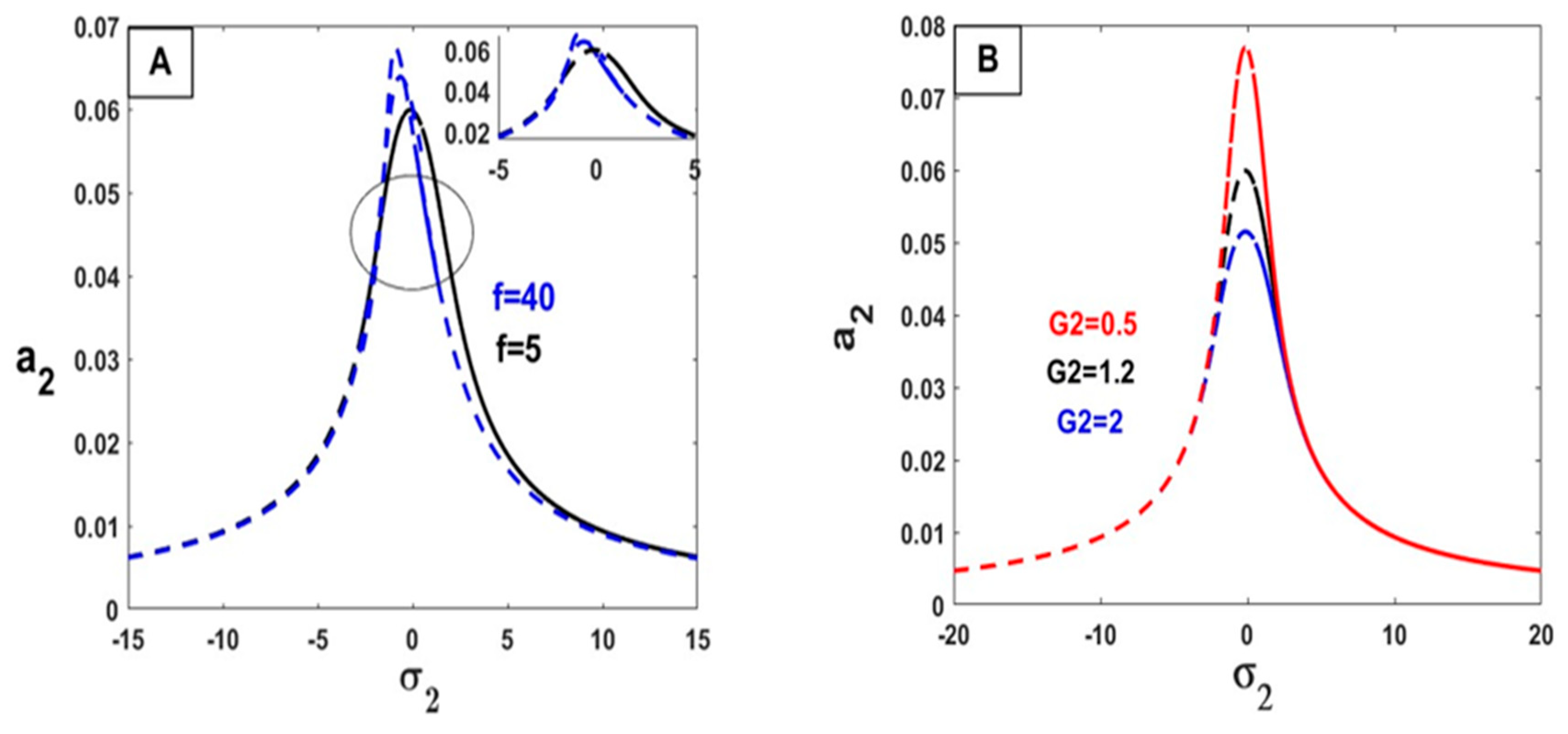
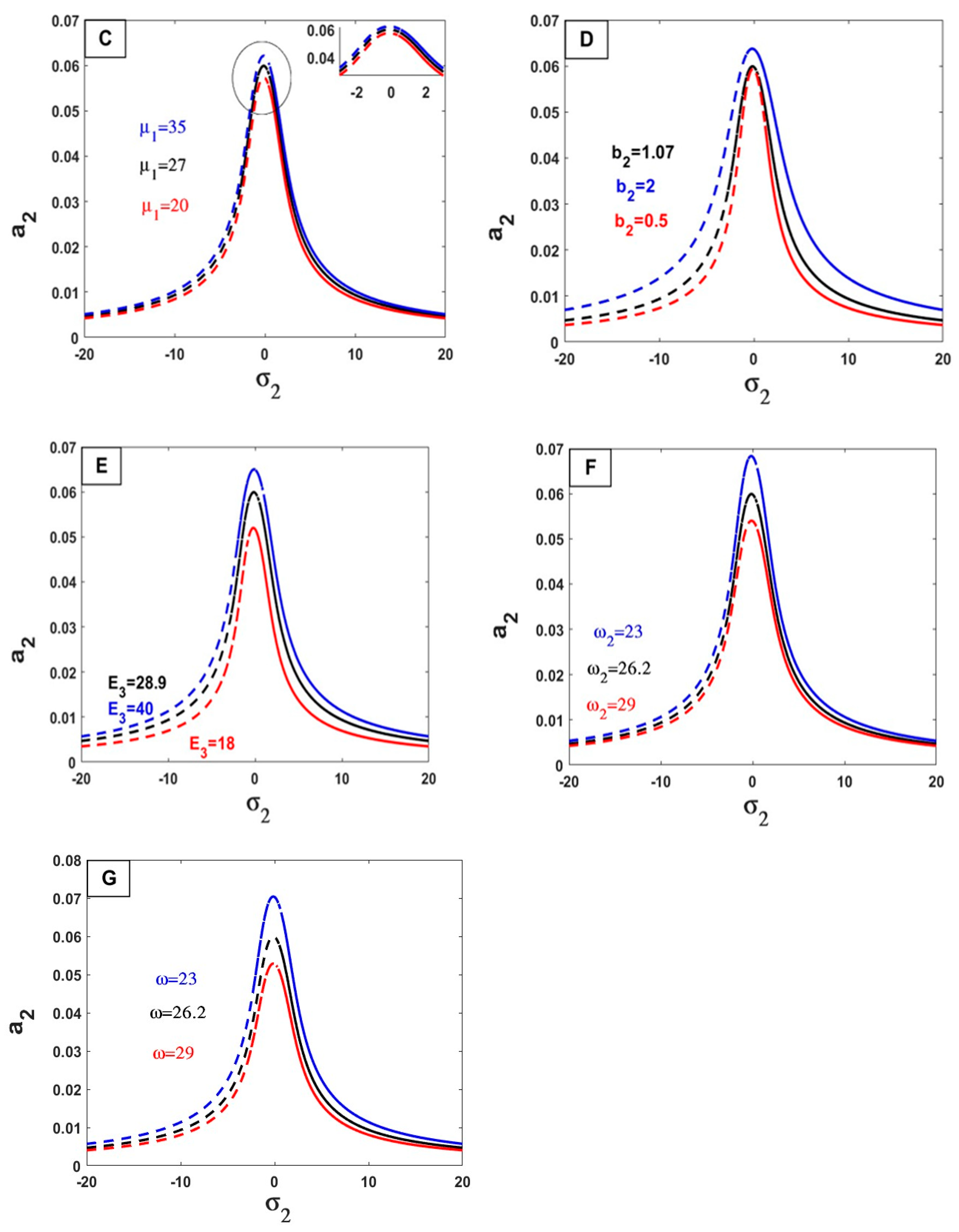
Effects of parameters on the response curves of stability of the steady-state amplitude against (stable: solid line, unstable: dashed line) (A) Effect , (B) Effect , (C) Effect , (D) Effect , (E) Effect , (F) Effect , (G) Effect .
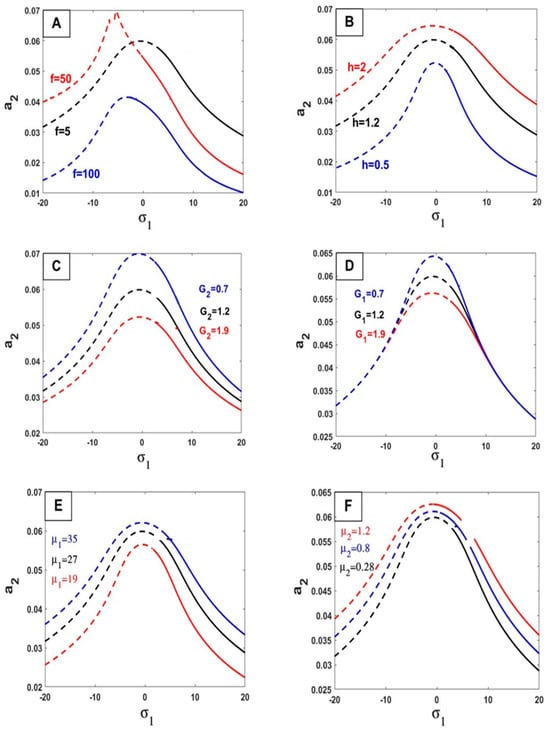
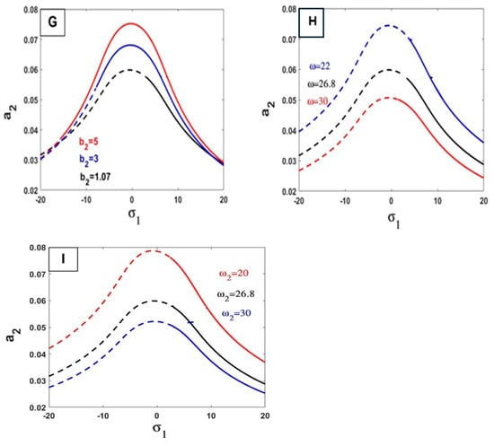
Figure 6.
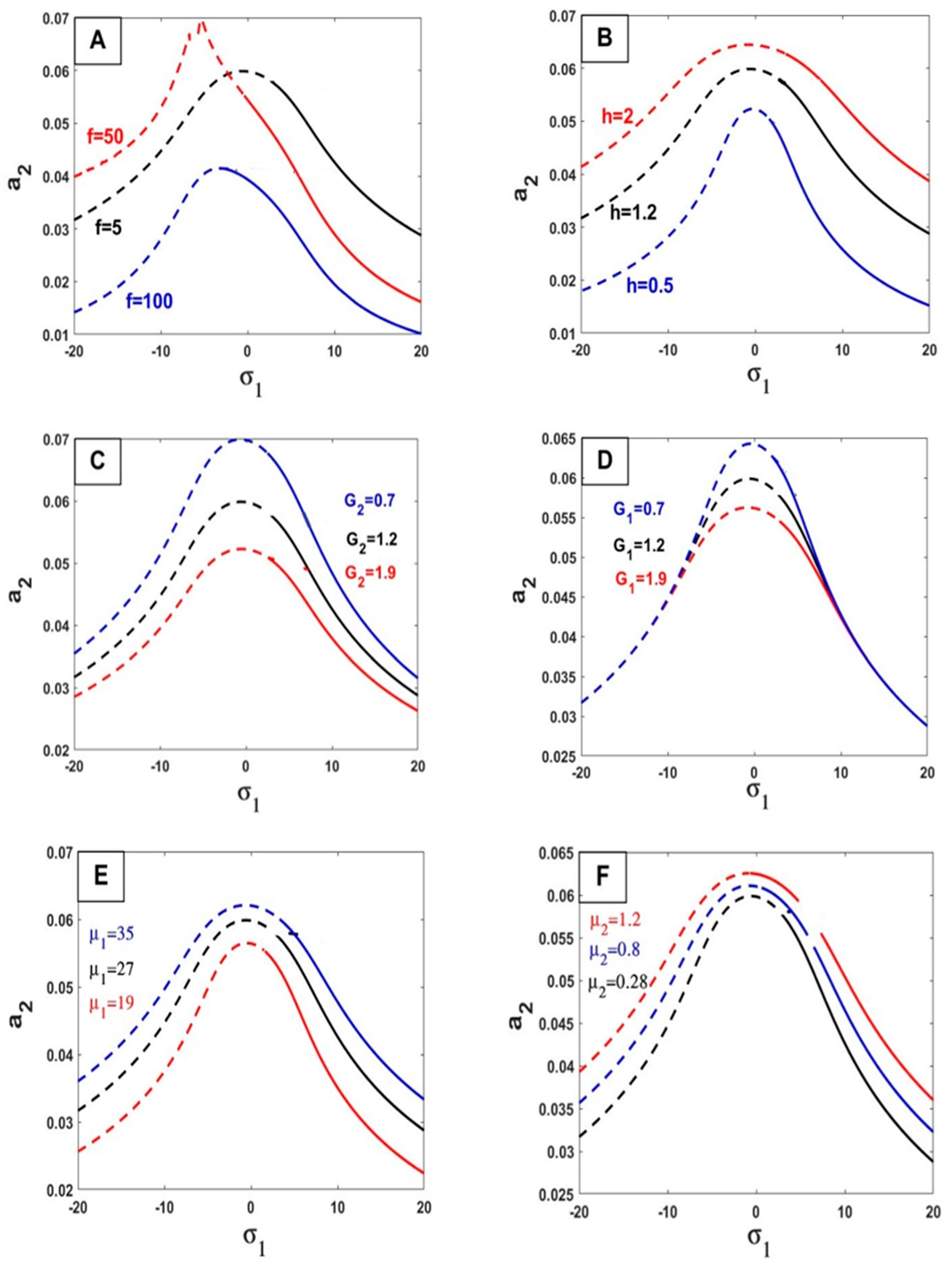
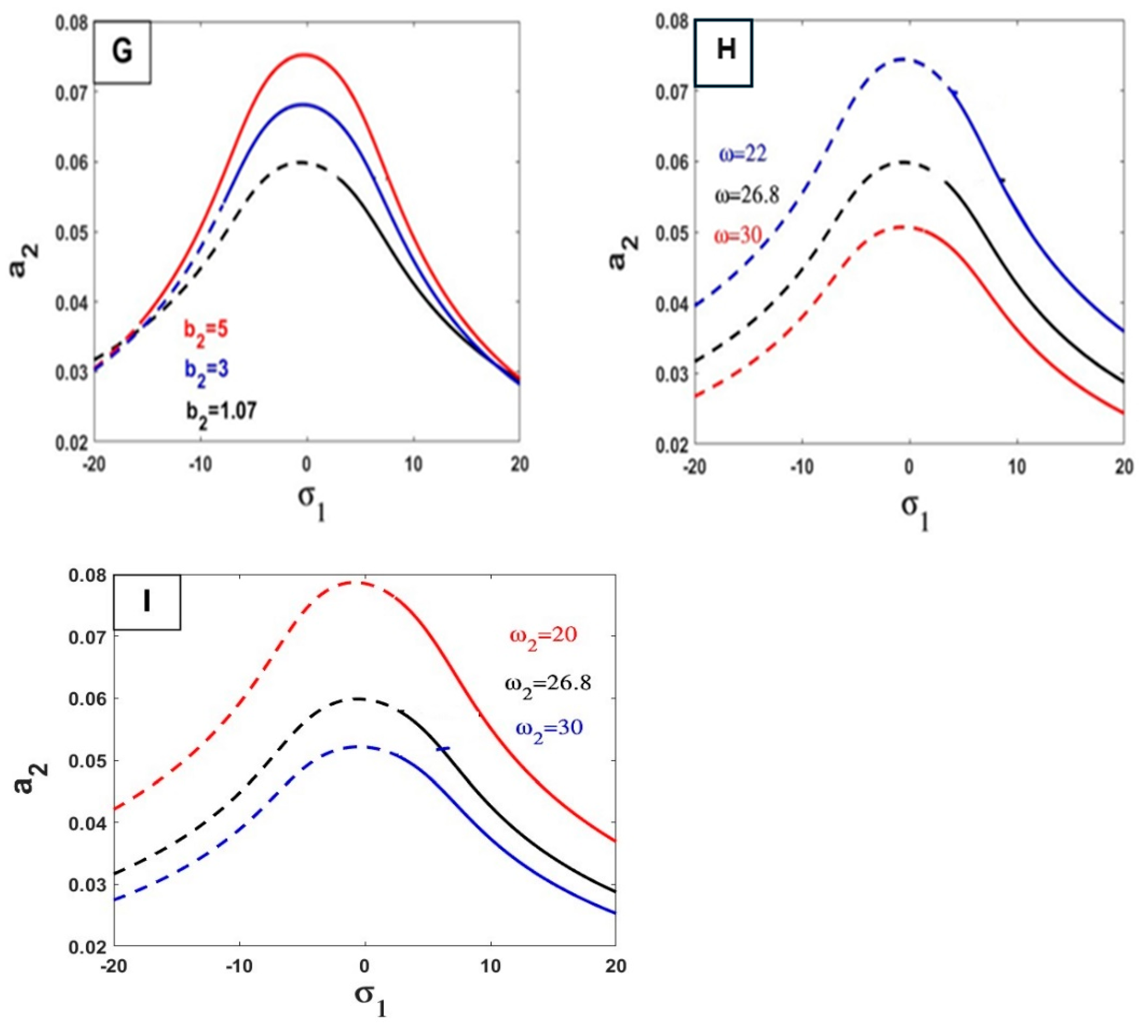
Effects of parameters on the response curves of stability of the steady-state amplitude against (stable: solid line, unstable: dashed line) (A) Effect , (B) Effect , (C) Effect , (D) Effect , (E) Effect , (F) Effect , (G) Effect , (H) Effect , (I) Effect .
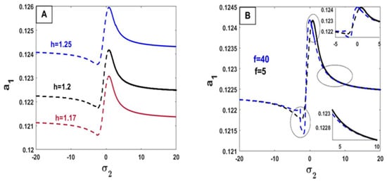

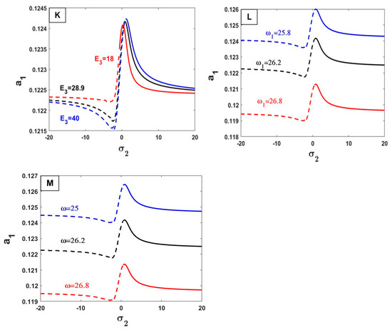
Figure 7.
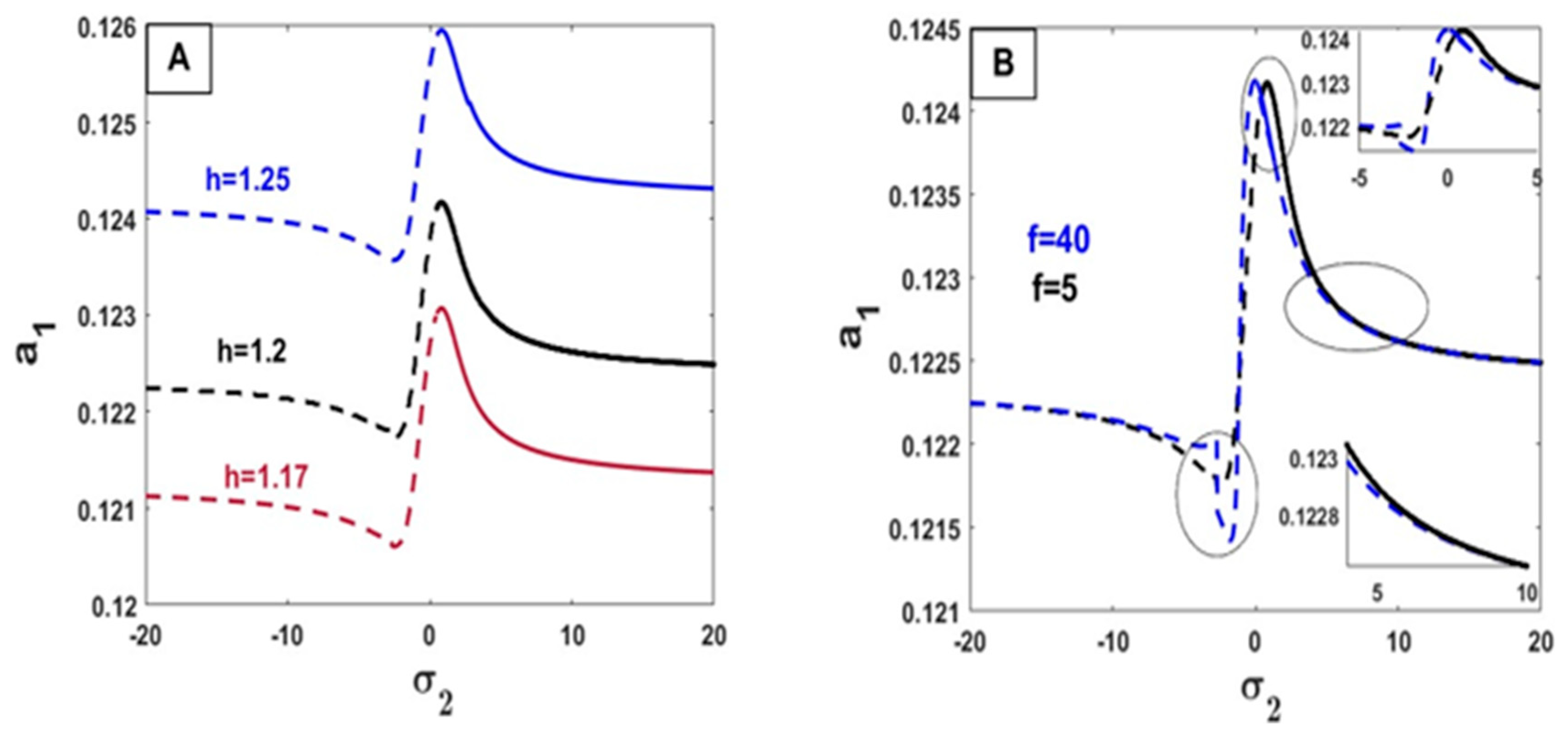
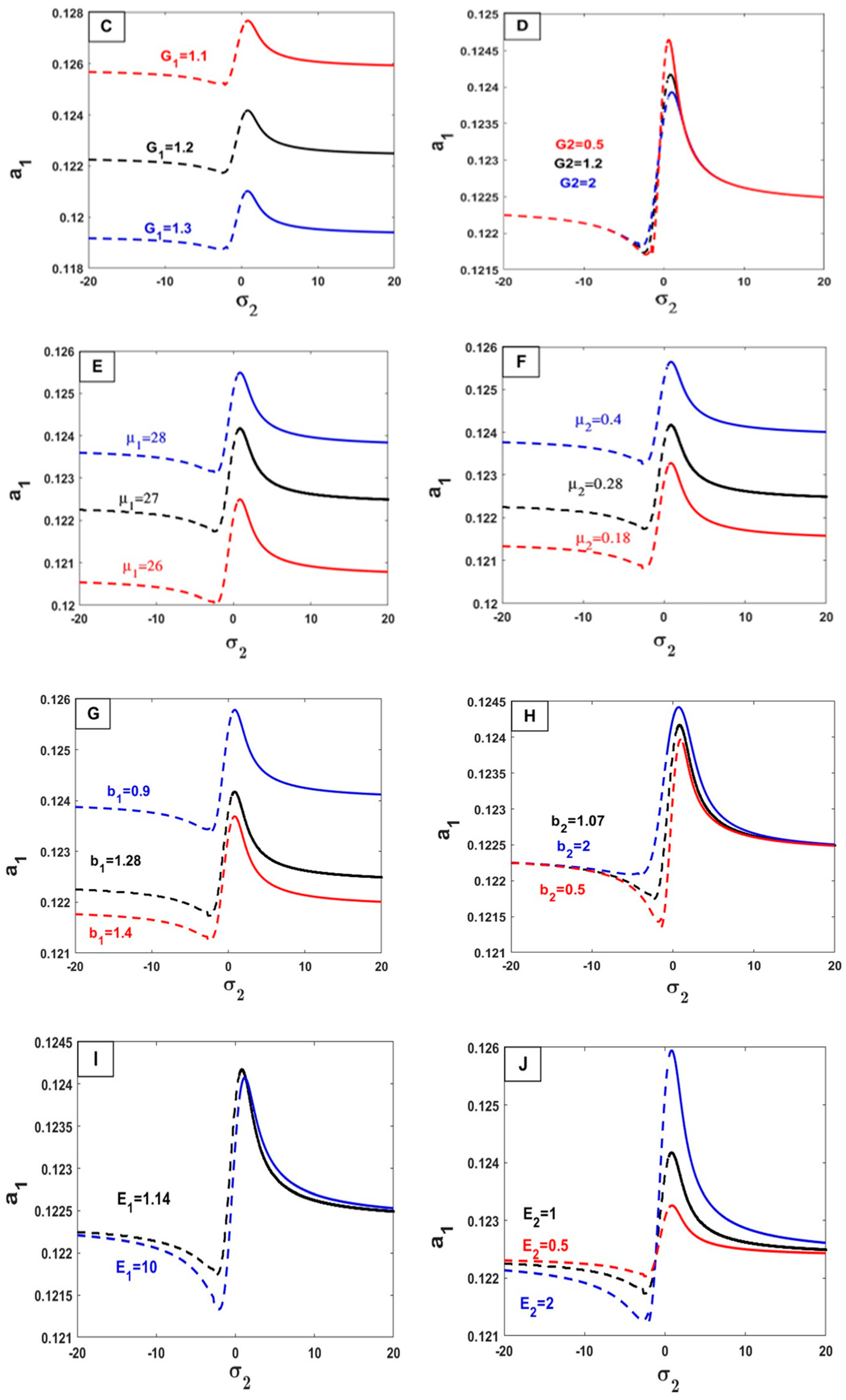
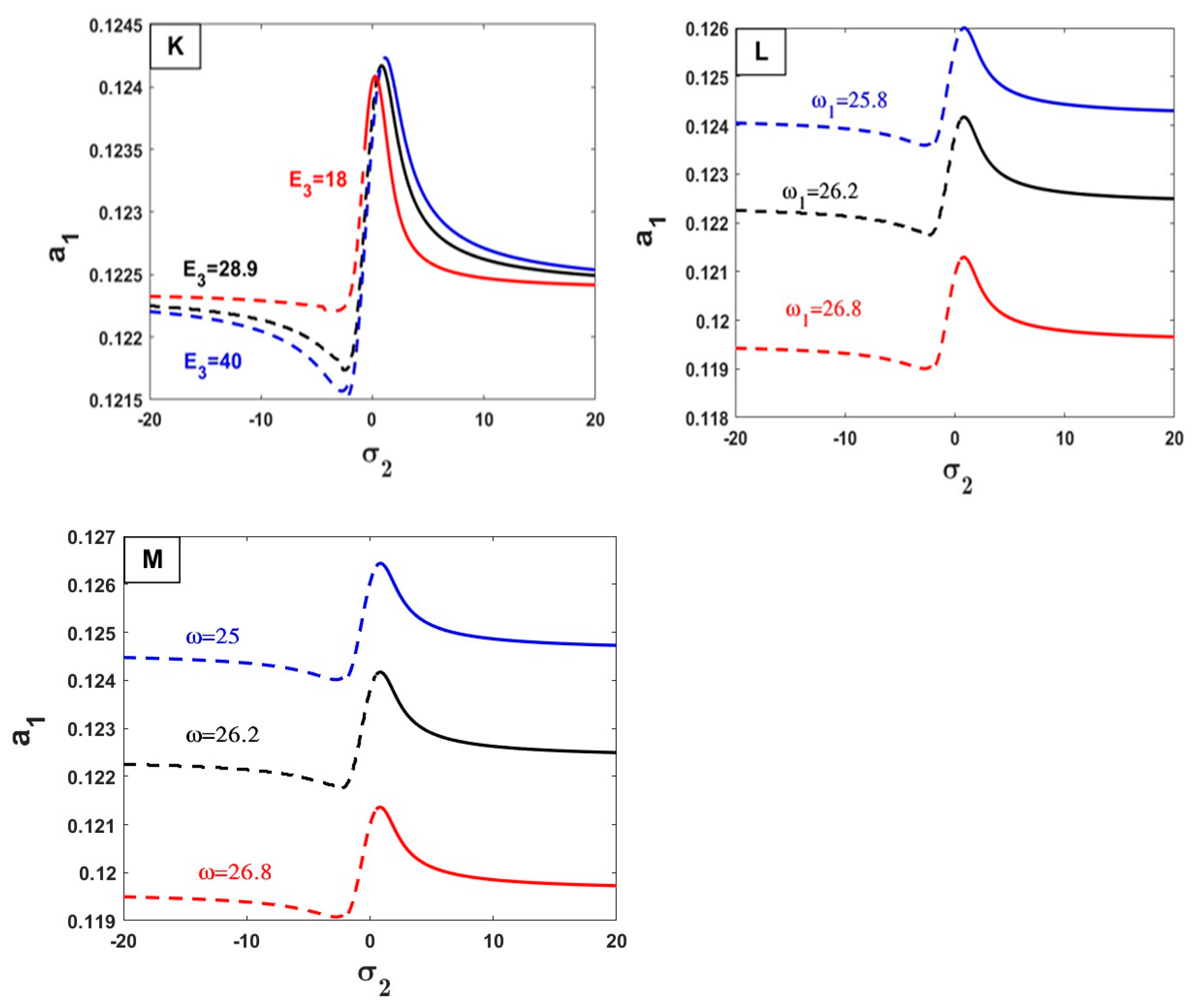
Parameter effects on the steady-state amplitude response curves of stability against (stable: solid line, unstable: dashed line) (A) Effect , (B) Effect , (C) Effect , (D) Effect , (E) Effect , (F) Effect , (G) Effect , (H) Effect , (I) Effect , (J) Effect , (K) Effect , (L) Effect , (M) Effect .

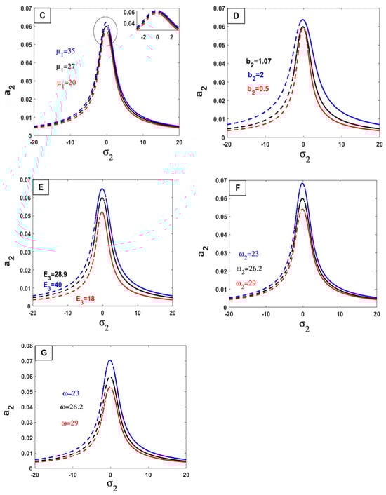
Figure 8.
Parameter effects on the steady-state amplitude response curves of stability against (stable: solid line, unstable: dashed line) (A) Effect , (B) Effect , (C) Effect , (D) Effect , (E) Effect , (F) Effect , (G) Effect .
Figure 4a shows the relation of against ; it shows as stable in the right branch and unstable in the left branch, and that the period of stability and instability changes. Figure 4b shows the relation of against ; it shows as stable in the right branch and unstable in the left branch, and that the period of stability and instability changes.
5.2. Effect of Different Parameters
We have concluded the following based on our examination of the extent to which variables alter the frequency curve and its impact on the periods of stability and instability, as shown in the accompanying Figure 5, Figure 6, Figure 7 and Figure 8 and explain the basic concepts and physical parameters.
- 1.
- Natural frequency . Since every body has mass and rigidity, all bodies have natural frequencies. Because of its interaction, the wave’s amplitude and frequency are physically inversely proportional to one another. The amplitude reduces as the frequency rises. The amplitude increases as the frequency decreases. The frequency of the oscillation has no bearing on its amplitude.
- 2.
- The process of releasing energy to halt vibratory motion, including mechanical oscillations, is known as damping in physics. Unless there is damage to the system controlled by the vibration, the amplitude steadily reduces with higher damping levels due to the increased damping () force within the elastic limit of mainframes.
- 3.
- An effect that operates on an object and changes its condition, direction, location, or movement is referred to be a force (f) in physics. This definition states that the relationship between amplitude and force is a removal relationship by which amplitude values are increased by force values.
- 4.
- Gain of control (): This indicates that the relationship is produced inversely by raising the values of the gain of control by lowering the amplitude. Gain of control is typically used to reduce vibration and damage to the dynamical system.
Based on all of these previous physical meanings, the validity of the following results in the study of the effects of these parameters on the frequency curve is confirmed.
In Figure 5, we studied the change in parameter values and their impact on the relationship between the response curves of stability of the steady-state amplitude a1 against . If the force increases significantly, it does not affect the increase or decrease in amplitude, but rather affects points of stability and instability. However, with a very large increase in force for external environmental conditions, the force can turn out to be a tranquilizer and reduce the frequency, as shown in Figure 5A. By increasing the values of the parameters () on Figure 5B,D,E, the value of the amplitude frequency increases. In other words, the opposite happens with these values () on Figure 5C,F,G; by increasing these values, the amplitude-frequency decreases. Finally, by increasing and decreasing the amplitude under effect of parameter the region of stable and unstable will change.
An increase in applied force can change the oscillation frequency in physical systems, especially in mechanical systems that vibrate or oscillate. To get this, think about the following two situations:
1. Spring–Mass system: The mass (m) and spring constant (k) of a basic mass–spring system determine the oscillation frequency (f) using the following formula:
In this system, the frequency is not directly impacted by increasing the applied force. On the other hand, the frequency may be affected if the applied force is so great that it permanently modifies the spring constant (k), for example by stretching the spring beyond its elastic limit.
2. Forced Oscillations and Damping: If an external force causes a system to oscillate at a particular frequency, a large increase in this force may cause non-linear effects or increase damping. Elevated damping has the capacity to modify the inherent frequency of the system by reducing the amplitude of oscillations. Extreme circumstances may cause non-linear forces to alter the system’s dynamics and the observed frequency.
In Figure 6, we showed the change in parameter values and their impact on the relationship between the response curves of stability of the steady-state amplitude against . If the force increases significantly, it does affect the increase in amplitude, but with a very large increase in force for external environmental conditions, the force can turn out to be a tranquilizer and reduce frequency, affecting points of stability and instability, as shown in Figure 6A. This is based on the explanation provided above. Therefore, while a direct increase in the force applied to the system leads to a fundamental change in frequency and shows an inverse relationship, as illustrated in the Figure when the force reaches a value higher than 60, and is clearly evident at a force value of 100, high forces can lead to effects or changes in damping that may reduce the effective frequency of the system. However, this is not permissible for the system as it diminishes the performance of the vehicle and affects its core tasks and movement. More propulsion force is required and higher costs are incurred, which highlights the importance and necessity of implementing control systems to achieve damping without relying on high forces as dampers. By increasing the values of the parameters () in Figure 6B,E–G, the value of the amplitude frequency increases, where this parameters express the following meanings (hump height, parameter of road, and negative damping). In other words, the opposite happens with these values through gain of control and natural frequency () on Figure 6C,D,H,I; by increasing these values, the amplitude frequency decreases. Finally by increasing and decreasing the amplitude under effect of parameter the region of stable and unstable will change.
In Figure 7, we show the change in parameter values and their impact on the relationship between the response curves of stability of the steady-state amplitude against . The effect of force on this part, even if it increases significantly, does not affect the amplitude much, as shown in Figure 7B. By increasing the values of the parameters () on Figure 7A,E,F,J,K, the frequency of the value of the amplitude increases. In other words, the opposite happens with these values () in Figure 7C,D,G,I,L,M, and with these values, the amplitude-frequency decreases.
In Figure 8, we show the change in parameter values and their impact on the relationship between the response curves of stability of the steady-state amplitude a2 against σ2. By increasing the values of the parameters () on Figure 8A,C,D,E, the value of the amplitude frequency increases. In other words, the opposite happens with these values () on Figure 8B,F,G, by increasing these values, the amplitude frequency decreases.
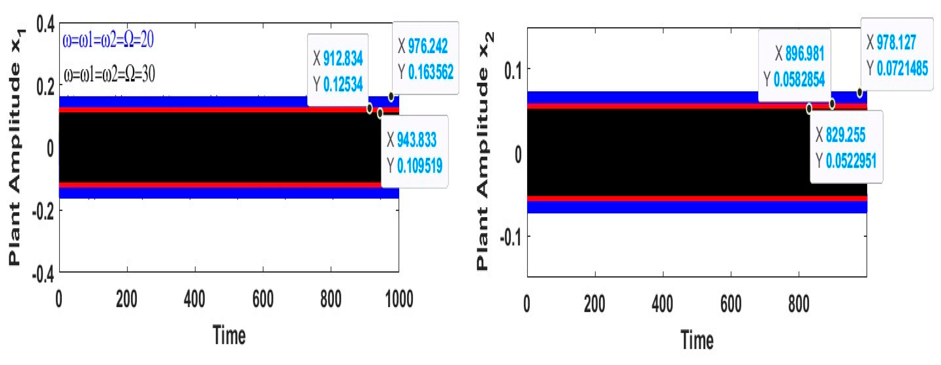
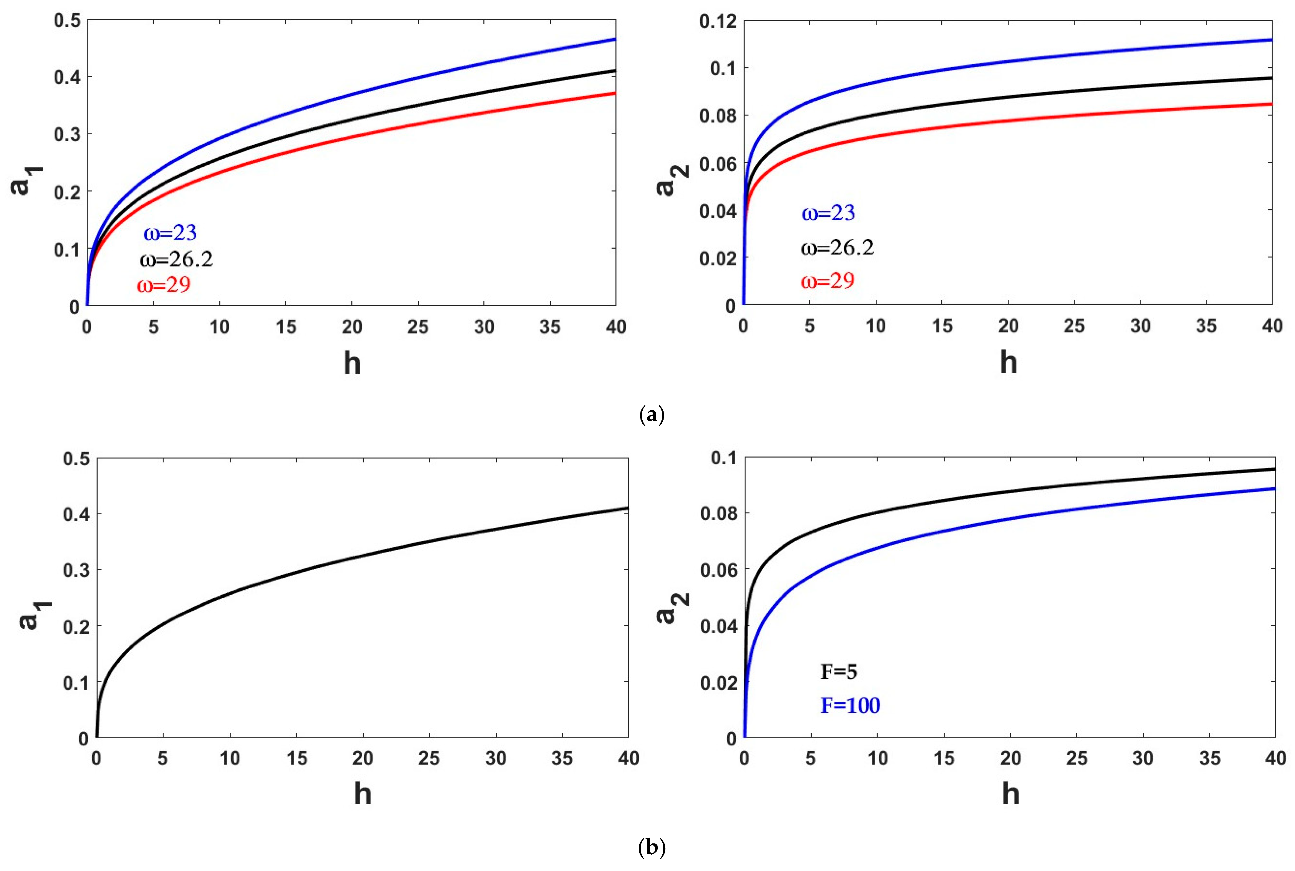
Figure 9 shows the effect of natural frequencies , the forcing frequency , and the displacement angular frequency of road at worst case with control. To prove the inverse relationship of these parameters with the value of the amplitude–frequency that appeared in the frequency curve while studying their effect on the curvature in the previous figures, and by comparing the values in Figure 9 and Figure 10, the relationship was achieved. The explanation for this is the presence of the bump equation, based on where the bump is represented as a simple harmonic motion .
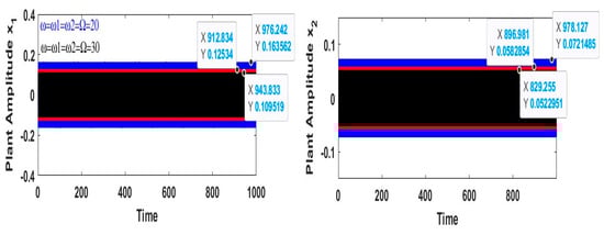
Figure 9.
Effect of parameter frequency at worst case with control on time history.
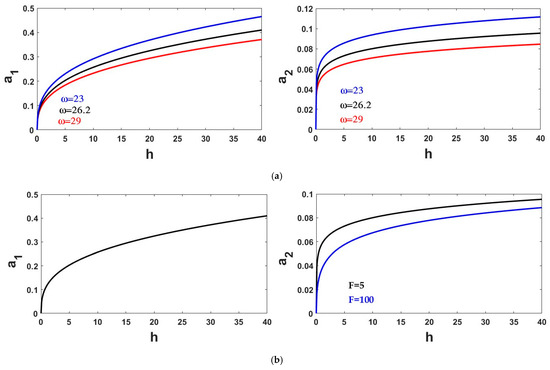
Figure 10.
Effect of the road parameter on the relation between the amplitude and h. (a) with (b) with .
6. Comparison
In this section, we conducted various types of comparisons, to demonstrate the validity of our studies.
6.1. Comparison of Types of Control
A comparison was made of the effectiveness of different controls and the best one representing the equation of motion to the road was a simple harmonic hump, as shown in the following figures.
Figure 11 displays the resulting effectiveness of two types of controls in the worst response case. Comparing these types, we were able to choose the control that has more effect on the system, in this case the hump expressed as step unit y = h where h is the height of the hump. As can be seen, the initial amplitude values before using the control were very small and there was no physical effect or benefit from using the control. Therefore, we decided to change the type of bump equation, as shown in the following figure.
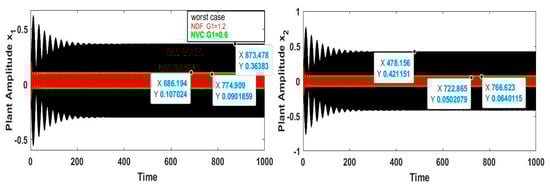
Figure 11.
Response of the system without absorber when hump constant step (y = h).
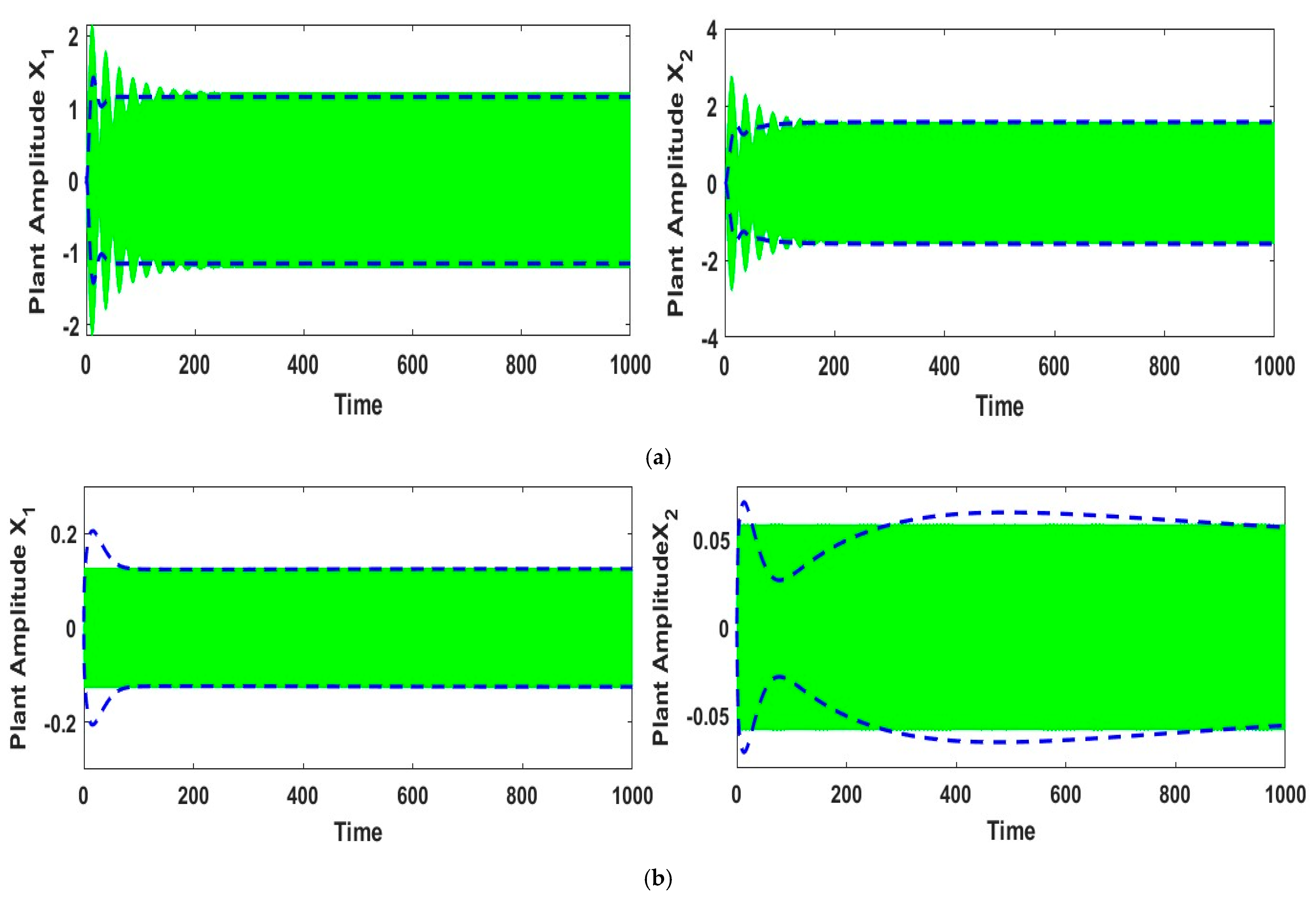
Figure 12 shows the result of multiple control methods applied to the worst case. By examining those types, we were able to choose the control that has a greater effect on the system, in this case a simple harmonic hump y = h sin () where h is the height of . Figure 12a studies PPF in two cases and Figure 12b studies CNVC and NDF; the results show that CNVC was the most effective, as shown in the figures above, since it was able to manage and minimize the vibration as much as it could.
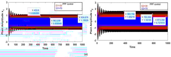
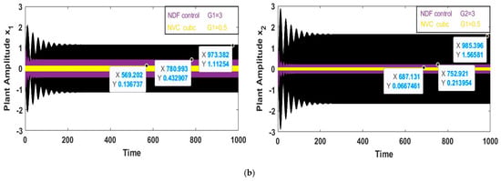
Figure 12.
Impacts on the system of multiple controls without absorber (black color) when hump represented as simple harmonic hump . (a) Effect of PPF in two cases (b) Effects of CNVC and NDF in two cases.
6.2. Comparison between the Numerical and Approximation Solutions
In Figure 13, we obtained perfect identification findings and nearly comparable results by comparing the numerical solution with the approximate solution.
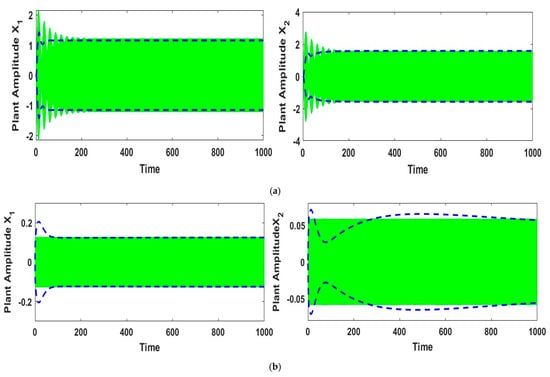
Figure 13.
Comparison between numerical solution (----------) and approximation solution (a) in worst case without control and (b) in worst case with control.
6.3. Comparison between Frequency Response Curves (FRC) and Time History Using RK-4
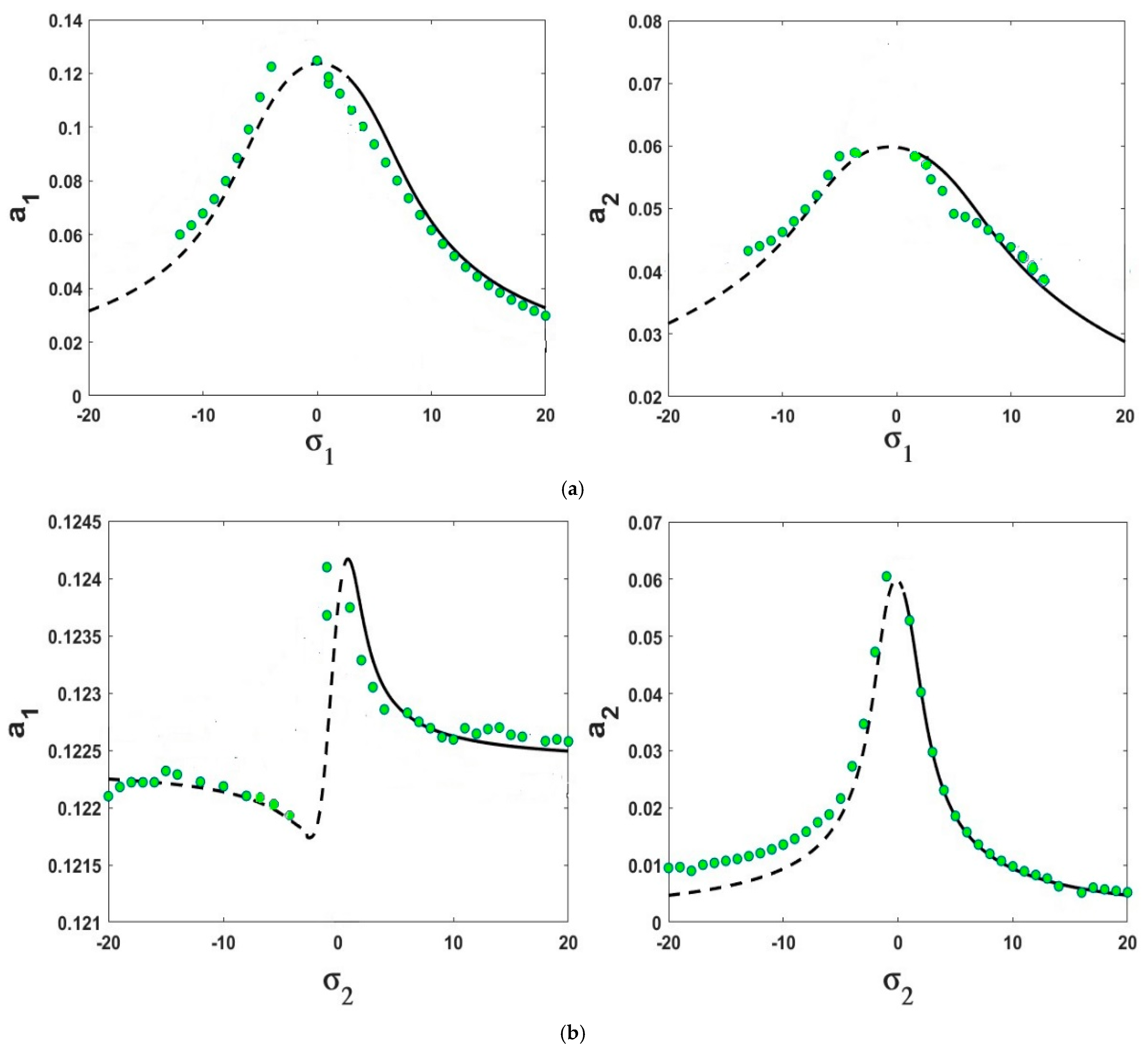
Figure 14 verifies the results of Figure 4a,b numerically; it can be seen that the numerical simulation results are in good agreement with the analytical solution results in two relations, against and against .
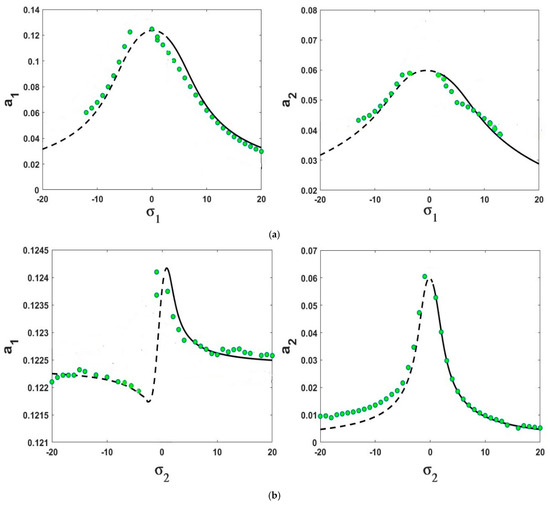
Figure 14.
Comparison between the numerical solution (green circles) and the approximation solution of the frequency curve (black color: solid line is stable and dashed line unstable) (a) relation between against ; (b) relation between against .
6.4. Comparison with Previous Studies
Reference [6] studied the effect of speed humps on the motion (displacement) of the car. The main research shows the effect of speed humps and the effects of the different parameters of the equation of motion for the road on the displacement of the car to know the appropriate dimensions of the road without mentioning or using any type of control systems. The goal was to arrive at the values of appropriate parameters with traffic, and we were able to connect those results according to numerical studies.
This article presents the quarter-car model with external excitation force to reduce vibrations by applying the Cubic Negative Velocity Control (CNVC) to effectively control vibration and reduce it to nearly a percentage of 2556%. Different types of control methods showing the effect of speed humps in the worst case were compared and the best control able to reduce of amplitude and damage on the car was selected. We also obtained a simple harmonic hump that is more effective on vibration for vehicles. Then, study of the changes effect of parameter values showed that the period of stability and instability changes with the different values of parameters, and the same goes for frequency values. The analysis demonstrates that the purpose of all calculations from the methodical solution is in excellent agreement with the numerical.
7. Conclusions
The response equation was displayed and an approximate solution was obtained using the approximation performed (averaging method) in the study. The system’s numerical behavior was examined in the study to determine the vibration’s amplitude value and the existence of the controller. To demonstrate the stability system, the phase plane methodology and the frequency response equation (also known as the averaging method) were applied simultaneously with the resonance case study to verify the numerical solution. The following results are given based on the previously identified study’s current implementation, affecting both the frequency response equations and results:
- 1.
- By comparing these types of controls, we were able to determine which one had a greater impact on the system in the case of a simple harmonic hump. Cubic NVC was found to be the most effective option because it could effectively control vibration and reduce it by nearly 2556%.
- 2.
- We obtained an excellent corresponding result and almost equal results by comparing the numerical solution with the approximate solution.
- 3.
- 4.
- We showed the change in parameter values and their impact on the relationship of the response curves of stability of the steady-state amplitude () against (), as shown in the figures.
- 5.
- The primary system’s steady-state amplitude grew monotonically, and when parameter values increased and reduced, the amplitude value decreased monotonically.
- 6.
- The effect of natural frequencies , the forcing frequency and displacement angular frequency of road at worst case with control were shown. To prove the inverse relationship of these parameters with the value of the amplitude–frequency that appeared in the frequency curve while studying their effect on the curvature in the previous Figures, the values in various Figures were compared.
- 7.
- Verifies the results of Figure 14a,b numerically; it can be seen that the numerical simulation results are in good agreement with the analytical solution result in two relations, against and against .
In order to improve passenger comfort and safety, future research could look into how cars behave and what effects they have under various road deformation systems, as well as how severe these effects are on traffic flow. Additionally, the technique could be used to improve the medical safety of ambulances, military vehicles in mountainous terrain, and complete semi-vehicle models.
Author Contributions
K.A.: resources, methodology, formal analysis, validation, visualization, and reviewing. Y.A.A.: Conceptualization, resources, methodology, writing—original draft preparation, visualization, reviewing, and editing. A.T.E.-S.: investigation, methodology, data curation, validation, reviewing, and editing. M.M.A.: formal analysis, validation, investigation, methodology, data curation, conceptualization, validation, reviewing and editing. All authors have read and agreed to the published version of the manuscript.
Funding
This research was funded by the Researchers Supporting Project, number (RSPD2024R588), King Saud University, Riyadh, Saudi Arabia.
Data Availability Statement
All data generated or analyzed during this study are included in this published article.
Acknowledgments
The authors extend their appreciation to Researchers Supporting Project number (RSPD2024R588), King Saud University, Riyadh, Saudi Arabia.
Conflicts of Interest
The authors have not revealed any conflicting interests.
Nomenclature
| Stiffness wheel system | |
| Stiffness of the main system (care body) | |
| Damping of wheel | |
| Damping of main system (care body) | |
| Displacements of wheel system and main system (care body) | |
| The second derivative of | |
| Natural frequencies | |
| The forcing frequency | |
| The amplitude of excitation of each linear oscillator | |
| Non-linear gains of the Cubic Negative Velocity controller | |
| The coordinates of simple harmonic motion of simple harmonic hump and velocity | |
| Hump height | |
| Displacement angular frequency | |
| Speed car | |
| Length of displacement for hump |
Appendix A
References
- Gobbi, M.; Levi, F.; Mastinu, G. Multi-objective stochastic optimisation of the suspension system of road vehicles. J. Sound Vib. 2006, 298, 1055–1072. [Google Scholar] [CrossRef]
- Khorshid, E.; Alfares, M. Model refinement and experimental evaluation for optimal design of speed humps. Int. J. Veh. Syst. Model. Test. 2007, 2, 80–99. [Google Scholar] [CrossRef]
- Amer, Y.A.; Bauomy, H.S.; Sayed, M. Vibration suppression in a twin-tail system to parametric and external excitations. Comput. Math. Appl. 2009, 58, 1947–1964. [Google Scholar] [CrossRef]
- Dai, J.; Gao, W.; Zhang, N. Random displacement and acceleration responses of vehicles with uncertainty. J. Mech. Sci. Technol. 2011, 25, 1221–1229. [Google Scholar] [CrossRef]
- El-Ganaini, W.A.; Saeed, N.A.; Eissa, M. Positive position feedback (PPF) controller for suppression of nonlinear system vibration. Nonlinear Dyn. 2013, 72, 517–537. [Google Scholar] [CrossRef]
- Hassaan, G.A. Car Dynamics using Quarter Model and Passive Suspension, Part II: A Novel Simple Harmonic Hump\n. IOSR J. Mech. Civ. Eng. 2015, 12, 93–100. [Google Scholar]
- Hassaan, G.A. Car Dynamics Using Quarter Model and Passive Suspension, Part III: A Novel Polynomial Hump. IOSR J. Mech. Civ. Eng. Ver. III 2015, 12, 2320–2334. [Google Scholar]
- Huang, C.; Zeng, J.; Luo, G.; Shi, H. Numerical and experimental studies on the car body flexible vibration reduction due to the effect of car body-mounted equipment. Proc. Inst. Mech. Eng. Part F J. Rail Rapid Transit 2018, 232, 103–120. [Google Scholar] [CrossRef]
- Silveira, M.; Wahi, P.; Fernandes, J.C.M. Effects of asymmetrical damping on a 2 DOF quarter-car model under harmonic excitation. Commun. Nonlinear Sci. Numer. Simul. 2017, 43, 14–24. [Google Scholar] [CrossRef]
- Ghasabi, S.A.; Shahgholi, M.; Arbabtafti, M. Analysis and suppression of the nonlinear oscillations of a continuous rotating shaft using an active time-delayed control. Mech. Adv. Mater. Struct. 2021, 28, 1978–1991. [Google Scholar] [CrossRef]
- Li, T.; Sun, W.; Meng, Z.; Huo, J.; Dong, J.; Wang, L. Dynamic investigation on railway vehicle considering the dynamic effect from the axle box bearings. Adv. Mech. Eng. 2019, 11, 1687814019840503. [Google Scholar] [CrossRef]
- Azimov, B.M.; Yakubjanova, D.K. Modeling and Optimal Control of Motion of cotton harvesting machines MX-1.8 and hitching systems of picking apparatus under vertical oscillations. J. Phys. Conf. Ser. 2019, 1210, 012004. [Google Scholar] [CrossRef]
- Azimov, B.M.; Abdazimov, A.D.; Sherkobilov, S.M.; Ikhsanova, S.Z. Modeling and numerical methods for studying the movement of a semi-mounted cotton harvesting machine. IOP Conf. Ser. Earth Environ. Sci. 2022, 1076, 012005. [Google Scholar] [CrossRef]
- Azimov, B.M.; Ikhsanova, S.Z. Mathematical modelling and numerical methods for studying the dynamic stability of the movement of cotton harvesters on slopes. E3S Web Conf. 2023, 386, 03005. [Google Scholar] [CrossRef]
- Dumitriu, M. Numerical study of the inuence of suspended equipment on ride comfort in high-speed railway vehicles. Sci. Iranica. 2020, 27, 1897–1915. [Google Scholar]
- Bauomy, H.S.; EL-Sayed, A.T. A time-delayed proportional-derivative controller for a dielectric elastomer circular membrane. Chinese J. Phys. 2023, 84, 216–231. [Google Scholar] [CrossRef]
- Łuczko, J.; Ferdek, U. Nonlinear dynamics of a vehicle with a displacement-sensitive mono-tube shock absorber. Nonlinear Dyn. 2020, 100, 185–202. [Google Scholar] [CrossRef]
- Stojanovic, N.; Jweeg, M.J.; Grujic, I.; Petrovic, M.; Muhsen, S.; Abdullah, O.I. An Investigation of the Suspension Characteristics of the Line Model of the Vehicle Using the Taguchi Method. Int. J. Appl. Mech. Eng. 2022, 27, 170–178. [Google Scholar] [CrossRef]
- Le, D.D.; Tran, H.N. Dynamic Behavior Analysis of the Bus with Two-stage Asymmetric Damper Using the Quarter Car Model Subjected to Transient Road Profile. J. Tech. Educ. Sci. 2023, 75A, 40–49. [Google Scholar] [CrossRef]
- Zhang, H.; Cheng, K.; Wang, E.; Rakheja, S.; Su, C.Y. Nonlinear Behaviors of a Half-Car Magneto- Rheological Suspension System Under Harmonic Road Excitation. IEEE Trans. Veh. Technol. 2023, 72, 8592–8600. [Google Scholar] [CrossRef]
- Wagh, S.Y. Quarter Car Rig for Software Function Development of Fully Active Suspension and Continuously Controlled Dampers. Master’s Thesis, Chalmers University of Technology, Gothenburg, Sweden, 2023. [Google Scholar]
- Alhelou, M.; Wassouf, Y.; Korzhukov, M.V.; Lobusov, E.S.; Serebrenny, V.V. Managing the Handling–Comfort Trade-Off in the Full Car Model by Active Suspension Control. Control. Sci. 2023, 1, 36–47. [Google Scholar]
- Shi, B.; Dai, W.; Yang, J. Performance enhancement of vehicle suspension system with geometrically nonlinear inerters. Arch. Appl. Mech. 2023, 94, 39–55. [Google Scholar] [CrossRef]
- Kandil, A.; Hamed, Y.S.; Alsharif, A.M.; Awrejcewicz, J. 2D and 3D visualizations of the Mass-damper-spring model dynamics controlled by a servo-controlled linear actuator. IEEE Access 2021, 9, 153012–153026. [Google Scholar] [CrossRef]
- Kandil, A.; Hamed, Y.S.; Abualnaja, K.M.; Awrejcewicz, J.; Bednarek, M. 1/3 order subharmonic resonance control of a mass-damper-spring model via cubic-position negative-velocity feedback. Symmetry 2022, 14, 685. [Google Scholar] [CrossRef]
- Kandil, A.; Hamed, Y.S.; Mohamed, M.S.; Awrejcewicz, J.; Bednarek, M. Third-order superharmonic resonance analysis and control in a nonlinear dynamical system. Mathematics 2022, 10, 1282. [Google Scholar] [CrossRef]
- Kandil, A.; Hamed, Y.S.; Awrejcewicz, J. Harmonic balance method to analyze the steady-state response of a controlled mass-damper-spring model. Symmetry 2022, 14, 1247. [Google Scholar] [CrossRef]
- Kandil, A.; Hamed, Y.S. Integral Resonant Controller for Suppressing Car’s Oscillations and Eliminating its Inherent Jump Phenomenon. Eur. J. Pure Appl. Math. 2023, 16, 2729–2750. [Google Scholar] [CrossRef]
- Darus, R.; Enzai, N.I. Modeling and control active suspension system for a quarter car model. In Proceedings of the 2010 International Conference on Science and Social Research (CSSR 2010), Kuala Lumpur, Malaysia, 5–7 December 2010; Institute of Electrical and Electronics Engineers (IEEE): New York, NY, USA; pp. 1203–1206. [Google Scholar]
- Al-Mutar, W.H.; Abdalla, T.Y. Quarter car active suspension system control using fuzzy controller tuned by pso. Int. J. Comput. Appl. 2015, 127, 38–43. [Google Scholar]
- Altinoz, O.T. Multiobjective PID controller design for active suspension system: Scalarization approach. Int. J. Optim. Control. Theor. Appl. (IJOCTA) 2018, 8, 183–194. [Google Scholar] [CrossRef]
- Basargan, H.; Mihály, A.; Gáspár, P.; Sename, O. Integrated adaptive velocity and semi-active suspension control for different road profiles. In Proceeding of the 2022 30th Mediterranean Conference on Control and Automation (MED), Vouliagmeni, Greece, 28 June 2022–1 July 2022; Institute of Electrical and Electronics Engineers (IEEE): New York, NY, USA; pp. 933–938. [Google Scholar]
- Abut, T.; Salkim, E. Control of quarter-car active suspension system based on optimized fuzzy linear quadratic regulator control method. Appl. Sci. 2023, 13, 8802. [Google Scholar] [CrossRef]


Disclaimer/Publisher’s Note: The statements, opinions and data contained in all publications are solely those of the individual author(s) and contributor(s) and not of MDPI and/or the editor(s). MDPI and/or the editor(s) disclaim responsibility for any injury to people or property resulting from any ideas, methods, instructions or products referred to in the content. |
© 2024 by the authors. Licensee MDPI, Basel, Switzerland. This article is an open access article distributed under the terms and conditions of the Creative Commons Attribution (CC BY) license (https://creativecommons.org/licenses/by/4.0/).