Assessing the Bridge Structure’s System Reliability Utilizing the Generalized Unit Half Logistic Geometric Distribution

Abstract

Reliability is now widely recognized across various industries, including manufacturing. This study investigates a system composed of five components, one of which is a bridge network. The components are assumed to follow the generalized unit half logistic geometric distribution (GUHLGD) with equal failure rates over time. The following three improvement methods are considered: reduction, cold duplication, and hot duplication. The reliability function and mean time to failure (MTTF) are employers liability equivalence factors (REFs). Additionally, the $\lambda$ fractiles of both the original and enhanced systems are obtained. Numerical results illustrate the effectiveness of these techniques, with cold duplication shown to be the most effective, offering higher reliability and MTTF compared to hot duplication. The enhanced system outperforms the original system overall.

1. Introduction

Numerous studies have explored various systems’ reliability and fundamental characteristics, as dependability is a critical concept employed across many sectors, especially in manufacturing (see [1,2,3,4,5,6,7,8]). These systems may consist of components with varying or constant failure rates over time. In particular, the bridge system is composed of independent, identical components with Weibull-distributed lifetimes arranged in a series-parallel configuration. Alghamdi and Percy (2017) [9] examined methods to enhance the reliability of such bridge systems. Also, Luo et al. [10] presented an overview of calculation methods of structural time-dependent reliability.

Ezzati and Rasouli [11], along with El-Faheem et al. [12], analyzed parallel systems and compound-series configurations using the linear exponential distribution for evaluation. Jaramillo et al. (2022) [13] investigated the integration of reliability principles into the design process to enhance the performance of electrical power transmission systems. This approach aims to ensure a more consistent and stable electricity flow. Luo et al. (2022) provided an overview of the reliability theory concerning time-dependent components, aiming to enhance structural performance by reducing the occurrence of failures. Alot of authors discussed the improved of system that included a bridge framework such as [14,15,16,17,18,19,20,21]. A study by Mustafa et al. [22] improved the effectiveness of a five-part system that included a bridge framework by implementing a gamma distribution. In another study, using the linear exponential distribution and a range of enhancement methods, Mustafa et al. [23] improved a series-parallel system. Additionally, Mustafa [24] investigated a series system’s reliability equivalent factor (REF) with failure rates following the Weibull and linearly increasing failure rate distributions. Mustafa (2009) [23] also investigated a series system’s reliability equivalent factor (REF) with failure rates conforming to Weibull and progressively rising failure-rate distributions. The reliability equivalence method was expanded by Mustafa and El-Faheem [25,26] by incorporating both the average and the equivalence of survival reliability. Moreover, Ramadan et al. (2024) [27] presented the reliability assessment of bridge structures using the Bilal distribution. This study examines the GUHLGD introduced by Nasiru et al. [28] in the units of the bridge framework system (Figure 1).

Assume that enhancements have been applied to all system components, encompassing reduction, duplication, and cold-improving methods.

In systems where minimizing size and weight is critical, such as well-logging equipment, pacemakers, biomedical devices, satellites, or other space applications, the redundancy method may not be the most effective solution [29]. In these cases, constraints on weight and space necessitate a focus on increasing component reliability rather than relying on redundancy. Therefore, greater attention must be focused on controlling the operational environment, ensuring stringent manufacturing quality control, and implementing robust design strategies. This leads to the application of the concept of reliability equivalency, wherein a system design optimized through reduction should be equivalent in reliability to one optimized using redundancy methods. According to this theory, alternative design approaches can enhance a system’s reliability; for more information, refer to [29]. In such cases, system designs can be compared using reliability metrics like the mean time to failure (MTTF) or the reliability function.

To determine the reliability equivalency factors (REFs) of specific systems, such as those described in [23,30], or to improve system reliability as discussed in [29,31,32,33,34,35,36], the literature explores the reliability equivalence technique for comparison of different designs [12,27,37]. This method identifies a representative service provider and constructs equivalent system components.

This research aims to derive the reliability equivalency factors for a universal series-parallel system. Various designs, including the original system and its enhanced versions, are evaluated using the reliability function and MTTF as performance measures to identify the required factors. Additionally, the flexibility of the generalized unit half logistic geometric distribution (GUHLGD) model in handling reliability data characteristics is highlighted. A case study is presented to demonstrate the model’s effectiveness in practical applications.

Section 2 introduces fundamental functions related to the GUHLGD. Section 3 discusses the bridge network system’s reliability and the MTTF functions. Section 4 describes various methods to improve the system, including reduction and hot and cold methods. In Section 5 and Section 6, the reliability equivalent factors (REFs) and $\lambda$ fractiles are derived. Finally, Section 7 reports the outcomes of the numerical analysis.

2. Fundamental Functions of the GUHLGD

The UHLGD was introduced by Ramadan et al. [28] to showcase its proficiency in managing data restricted in the interval $(0,1)$. In (2023) Baaqeel et al. [37] used the UHLGD to assess the system reliability of the bridge structure, and Nasiru et al. [28] presented the GUHLGD.

A random variable denoted as T is characterized as having a pdf (probability density function) that adheres to the GUHLGD, as represented below:

$$f\left(t\right)={\displaystyle \frac{2\alpha \theta t^{\theta -1}}{{\left(\left(\alpha -2\right)t^{\theta }-\alpha \right)}^2}},\alpha ,\theta >0,0<t<1,$$

(1)

and its cdf (cumulative distribution function) is denoted as

$$F\left(t\right)=1-{\displaystyle \frac{\alpha \left(1-t^{\theta }\right)}{\left(2-\alpha \right)t^{\theta }+\alpha }},\alpha ,\theta >0,0<t<1,$$

(2)

where $\alpha$ and $\theta$ are the scale and shape parameter, respectively.

Figure 2 depicts the cdf and the pdf of the GUHLGD across various $\alpha$ and $\theta$ values. The shapes of the pdf show that it can exhibit unimodal, reversed-J, bathtub, symmetric, right-skewed, and left-skewed shapes, as shown in Figure 2.

In addition, the GUHLGD’s survival ($S\left(t\right)$) and hazard failure-rate ($h\left(t\right)$) functions are expressed as

$$S\left(t\right)=1-F\left(t\right)={\displaystyle \frac{\alpha \left(1-t^{\theta }\right)}{\left(2-\alpha \right)t^{\theta }+\alpha }},\alpha ,\theta >0,0<t<1,$$

(3)

$$h\left(t\right)={\displaystyle \frac{f\left(t\right)}{S\left(t\right)}}={\displaystyle \frac{2\theta t^{\theta -1}}{\left(t^{\theta }-1\right)\left(\left(\alpha -2\right)t^{\theta }-\alpha \right)}},\alpha ,\theta >0,0<t<1.$$

(4)

Figure 3 displays the survival and the hazard functions of the GUHLGD for various $\theta$ and $\alpha$ values. The limiting behavior of the HRFalso suggests that it can have multiple shapes, such as bathtub, increasing, and N-shaped, as shown in Figure 3. It is worth indicating that the pdfdoes not exhibit symmetric, left-skewed, right-skewed, or bathtub shapes. Furthermore, the HRF lacks an N shape.

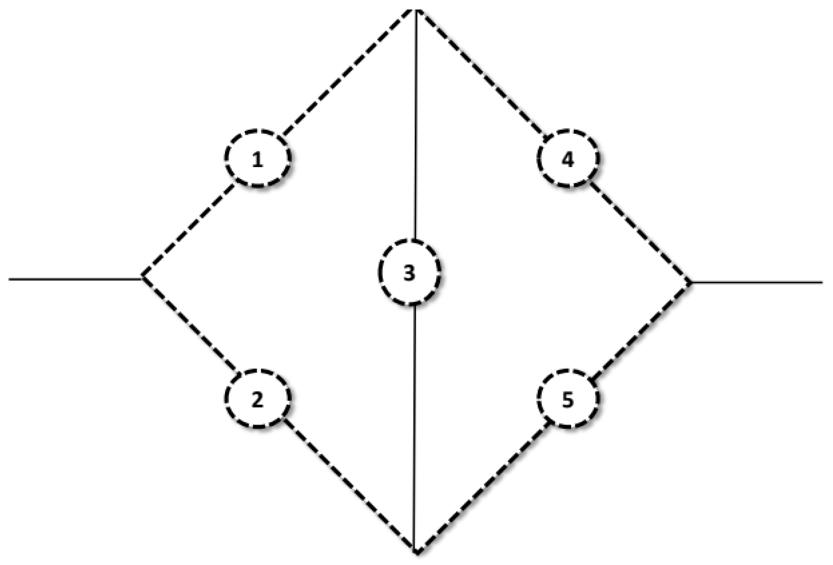
3. The Bridge System’s Reliability and the MTTF

The bridge system consists of five key components, one of which is a bridge network, as depicted in Figure 1. Each component is assumed to be independent and follows the generalized unit half logistic geometric distribution (GUHLGD) with parameters of $\alpha$ and $\theta$. In Equation (3), when time (t) is treated as the random variable, the survival function becomes the reliability function. The reliability function for component i, which is denoted as $r_i\left(t\right)$, where $i=1,2,\dots ,5$, is defined as follows:

$$r_i\left(t\right)={\displaystyle \frac{\alpha (1-t^{\theta })}{\left(2-\alpha \right)t^{\theta }+\alpha }},\alpha ,\theta >0,0<t<1.$$

(5)

The minimal path technique is a highly effective tool in network design and reliability analysis, providing a systematic approach to identifying and optimizing the most reliable paths within a system. This method is extensively applied across various fields to improve system robustness and performance. Here, the minimal path strategy is employed because it focuses on pinpointing the most reliable paths, simplifying the analysis of complex networks, and aiding in the design of systems with higher reliability by emphasizing critical paths. The minimal path technique for the bridge structure is depicted in Figure 4, where ${\tau }_i$ (with i ranging from 1 to 4) represents the minimal tie sets.

Let us define the set of all components in the system as $N=\{1,2,3,4,5\}$. For any given component (i), we define $N_{i^{\prime }}$ as the set containing all components except component i, meaning $N_{i^{\prime }}$ excludes component i from the system. The minimal path technique aids in identifying the critical combinations of components that are essential for the system’s proper functioning. Using this method, the system’s reliability function, denoted by $R\left(t\right)$, can be expressed as follows:

$$\begin{array}{cc}\hfill R\left(t\right)=& \sum _{i=1}^{4}P\left({\tau }_i\right)-\sum _{i=1}^3\sum _{j=i+1}^{4}P({\tau }_i\cap {\tau }_j)+\sum _{i=1}^2\sum _{j=i+1}^3\sum _{k=j+1}^{4}P({\tau }_i\cap {\tau }_j\cap {\tau }_k)\hfill \\ \hfill & -P\left(\bigcap _{i=1}^4{\tau }_i\right)=r_1\left(t\right)r_4\left(t\right)+r_2\left(t\right)r_5\left(t\right)+r_1\left(t\right)r_3\left(t\right)r_5\left(t\right)+\hfill \\ \hfill & r_2\left(t\right)r_3\left(t\right)r_4\left(t\right)-\sum _{i=1}^5\prod _{j\in N_{i^{\prime }}}{r}_i\left(t\right)+2\prod _{j\in N}{r}_j\left(t\right).\hfill \end{array}$$

(6)

Substituting the expression from Equation (5) into (6), we obtain the following:

$$R\left(t\right)=r^2\left(t\right)\left(r\left(t\right)\left(r\right(t)-2)\left(2r\right(t)-1)+2\right),$$

$$r^2\left(t\right)={\left({\displaystyle \frac{\alpha (1-t^{\theta })}{\alpha +(2-\alpha )t^{\theta }}}\right)}^2,$$

$$r\left(t\right)-2={\displaystyle \frac{\alpha (1-t^{\theta })}{\alpha +(2-\alpha )t^{\theta }}}-2={\displaystyle \frac{\alpha (1-t^{\theta })-2(\alpha +(2-\alpha )t^{\theta })}{\alpha +(2-\alpha )t^{\theta }}}={\displaystyle \frac{\alpha (1-t^{\theta })-2\alpha -4t^{\theta }+2\alpha t^{\theta }}{\alpha +(2-\alpha )t^{\theta }}}$$

$$={\displaystyle \frac{\alpha -\alpha t^{\theta }-2\alpha -4t^{\theta }+2\alpha t^{\theta }}{\alpha +(2-\alpha )t^{\theta }}}={\displaystyle \frac{-\alpha -4t^{\theta }+\alpha t^{\theta }}{\alpha +(2-\alpha )t^{\theta }}},$$

and

$$2r\left(t\right)-1=2\left({\displaystyle \frac{\alpha (1-t^{\theta })}{\alpha +(2-\alpha )t^{\theta }}}\right)-1={\displaystyle \frac{2\alpha (1-t^{\theta })}{\alpha +(2-\alpha )t^{\theta }}}-1={\displaystyle \frac{2\alpha (1-t^{\theta })-(\alpha +(2-\alpha )t^{\theta })}{\alpha +(2-\alpha )t^{\theta }}}$$

$$={\displaystyle \frac{2\alpha -2\alpha t^{\theta }-\alpha -(2-\alpha )t^{\theta }}{\alpha +(2-\alpha )t^{\theta }}}={\displaystyle \frac{2\alpha -\alpha -2\alpha t^{\theta }-2t^{\theta }+\alpha t^{\theta }}{\alpha +(2-\alpha )t^{\theta }}}$$

$$={\displaystyle \frac{\alpha -2\alpha t^{\theta }-2t^{\theta }+\alpha t^{\theta }}{\alpha +(2-\alpha )t^{\theta }}},$$

then

$$R\left(t\right)={\displaystyle \frac{2{(1-t^{\alpha })}^5{\alpha }^5}{{\left(t^{\theta }(2-\alpha )+\alpha \right)}^5}}-{\displaystyle \frac{5{(1-t^{\alpha })}^4{\alpha }^4}{{\left(t^{\theta }(2-\alpha )+\alpha \right)}^4}}+{\displaystyle \frac{2{(1-t^{\alpha })}^3{\alpha }^3}{{\left(t^{\theta }(2-\alpha )+\alpha \right)}^3}}+{\displaystyle \frac{2{(1-t^{\alpha })}^2{\alpha }^2}{{\left(t^{\theta }(2-\alpha )+\alpha \right)}^2}}.$$

(7)

Furthermore, the MTTF is expressed as follows:

$$MTTF\left(t\right)={\int }_0^{\infty }R\left(t\right)dt.$$

(8)

The Mathematica program was used to calculate the MTTF quantitatively.

4. Methods for Enhancing Performance

In this section, we improve the bridge system’s efficiency by employing the following methods to improve select components:

4.1. Reduction-Based Improvement Method

In this method, the system’s failure rate is reduced by scaling down the failure rates of individual components by a factor of $\rho$, where $0<\rho <1$. This reduction method is an effective approach for enhancing system reliability by systematically lowering the failure rates of its components. By applying the scaling factor ($\rho$), the overall system reliability is improved, and the mean time to failure (MTTF) is extended, yielding significant advantages in operational efficiency and cost savings.

Let A denote the set of components that have undergone this enhancement. For each component (i, where $i=1,2,3,4,5$), we define $h_i^{\rho }\left(t\right)$ as the hazard rate and $r_i^{\rho }\left(t\right)$ as the reliability function after the enhancement. These expressions are given as follows:

$$h_i^{\rho }\left(t\right)={\displaystyle \frac{2\theta \rho t^{\theta -1}}{(1-t^{\theta })(\alpha +(2-\alpha )t^{\theta })}},$$

(9)

$$r_i^{\rho }\left(t\right)=e^{-{\int }_0^t{h}_i^{\rho }\left(u\right)du}={\left({\displaystyle \frac{\alpha (1-t^{\theta })}{\left(2-\alpha \right)t^{\theta }+\alpha }}\right)}^{\rho }.$$

(10)

When applying this method to enhance the components within the set (A), think of $R_A^{\rho }$ as the reliability function of the improved system. The expression for $R_A^{\rho }$ can be described as follows:

• $A\in S_1=\left\{\left\{3\right\}\right\}$

  $$R_{A,S_1}^{\rho }\left(t\right)=2{\left(r\left(t\right)\right)}^2+2{\left(r\left(t\right)\right)}^2{r}_{\rho }-\sum _{i=1}^5\prod _{j\in N_{i^{\prime }}}{r}_i\left(t\right)+2\prod _{j\in N}{r}_j\left(t\right),$$

  then

  $$\begin{array}{cc}\hfill R_{A,S_1}^{\rho }\left(t\right)& ={\displaystyle \frac{{\alpha }^2{(t^{\alpha }-1)}^2\left(2t^{2\theta }{(\alpha -2)}^2(1+r_{\rho })-4\alpha t^{\theta }(\alpha -2)(1+r_{\rho }{t}^{\alpha })\right)}{{\left(\alpha -t^{\theta }(\alpha -2)\right)}^4}}\hfill \\ \hfill & +{\displaystyle \frac{{\alpha }^2{(t^{\alpha }-1)}^2\left({\alpha }^2(1+t^{\alpha }(2+(2t^{\alpha }{r}_{\rho }-1)))\right)}{{\left(\alpha -t^{\theta }(\alpha -2)\right)}^4}},\hfill \end{array}$$

  (11)
• $A\in S_2=\{\left\{1\right\},\left\{2\right\},\left\{4\right\},\left\{5\right\}\}$

  $$R_{A,S_2}^{\rho }\left(t\right)=r_{\rho }r\left(t\right)+{\left(r\left(t\right)\right)}^2+r_{\rho }{\left(r\left(t\right)\right)}^2+{\left(r\left(t\right)\right)}^3-\sum _{i=1}^5\prod _{j\in N_{i^{\prime }}}{r}_i\left(t\right)+2\prod _{j\in N}{r}_j\left(t\right),$$

  then

  $$\begin{array}{cc}\hfill R_{A,S_2}^{\rho }\left(t\right)& ={\displaystyle \frac{\alpha (t^{\alpha }-1)\left(r_{\rho }{((\alpha -2)t^{\theta }-\alpha )}^3-{\alpha }^2(4r_{\rho }-1){(t^{\alpha }-1)}^2((\alpha -2)t^{\theta }-\alpha )\right)}{{\left(\alpha -(\alpha -2)t^{\theta }\right)}^4}}\hfill \\ \hfill & +{\displaystyle \frac{\alpha (t^{\alpha }-1)\left({\alpha }^3(2r_{\rho }-1){(t^{\alpha }-1)}^3\right)\left(\alpha (t^{\alpha }-1)(1+r_{\rho }){\left(\alpha -(\alpha -2)t^{\theta }\right)}^2\right)}{{\left(\alpha -(\alpha -2)t^{\theta }\right)}^4}},\hfill \end{array}$$

  (12)
• $A\in S_3=\{\{1,3\},\{2,3\},\{3,4\},\{3,5\}\}$

  $$R_{A,S_3}^{\rho }\left(t\right)=r_{\rho }r\left(t\right)+{\left(r\left(t\right)\right)}^2+{\left(r_{\rho }\right)}^{2}r\left(t\right)+r_{\rho }r\left(t\right)-\sum _{i=1}^5\prod _{j\in N_{i^{\prime }}}{r}_i\left(t\right)+2\prod _{j\in N}{r}_j\left(t\right),$$

  then

  $$\begin{array}{cc}\hfill R_{A,S_3}^{\rho }\left(t\right)& ={\displaystyle \frac{\alpha (t^{\alpha }-1)\left(r_{\rho }{t}^{2\theta }{(\alpha -2)}^2(1+r_{\rho })-\alpha (\alpha -2)t^{\theta }\left(3r_{\rho }-r_{\rho }^2+t^{\alpha }(-1+r_{\rho }(3r_{\rho }-1))\right)\right)}{{\left((\alpha -2)t^{\theta }-\alpha \right)}^3}}\hfill \\ \hfill & +{\displaystyle \frac{\alpha (t^{\alpha }-1)\left({\alpha }^2\left(1+t^{\alpha }\left(-1+r_{\rho }(3-r_{\rho }+2t^{\alpha }(-1+r_{\rho }))\right)\right)\right)}{{\left((\alpha -2)t^{\theta }-\alpha \right)}^3}},\hfill \end{array}$$

  (13)
• $A\in S_4=\{\{1,5\},\{2,4\}\}$

  $$R_{A,S_4}^{\rho }\left(t\right)=2r_{\rho }r\left(t\right)+{\left(r_{\rho }\right)}^{2}r\left(t\right)+{\left(r\left(t\right)\right)}^3-\sum _{i=1}^5\prod _{j\in N_{i^{\prime }}}{r}_i\left(t\right)+2\prod _{j\in N}{r}_j\left(t\right),$$

  then

  $$\begin{array}{cc}\hfill R_{A,S_4}^{\rho }\left(t\right)& ={\displaystyle \frac{\alpha (t^{\alpha }-1)\left(r_{\rho }{t}^{2\theta }(2+r_{\rho }){(\alpha -2)}^2-\alpha (\alpha -2)t^{\theta }{r}_{\rho }\left(4+r_{\rho }(3t^{\alpha }-1))\right)\right)}{{\left((\alpha -2)t^{\theta }-\alpha \right)}^3}}\hfill \\ \hfill & +{\displaystyle \frac{\alpha (t^{\alpha }-1)\left({\alpha }^2\left(1+t^{\alpha }\left(-2+t^{\alpha }+r_{\rho }(4-r_{\rho }+2t^{\alpha }(-1+r_{\rho }))\right)\right)\right)}{{\left((\alpha -2)t^{\theta }-\alpha \right)}^3}},\hfill \end{array}$$

  (14)
• $A\in S_5=\{\{1,2\},\{4,5\}\}$

  $$R_{A,S_5}^{\rho }\left(t\right)=r_{\rho }r\left(t\right)+r_{\rho }r\left(t\right)+2r_{\rho }{\left(r\left(t\right)\right)}^2-\sum _{i=1}^5\prod _{j\in N_{i^{\prime }}}{r}_i\left(t\right)+2\prod _{j\in N}{r}_j\left(t\right),$$

  then

  $$\begin{array}{cc}\hfill R_{A,S_5}^{\rho }\left(t\right)& ={\displaystyle \frac{\alpha r_{\rho }(t^{\alpha }-1)\left(2t^{2\theta }{(\alpha -2)}^2-t^{\theta }\left(6-2t^{\alpha }+3r_{\rho }(t^{\alpha }-1)\right)\right)}{{\left((\alpha -2)t^{\theta }-\alpha \right)}^3}}\hfill \\ \hfill & +{\displaystyle \frac{\alpha r_{\rho }(t^{\alpha }-1)\left(\alpha (\alpha -2)+{\alpha }^2\left(2-r_{\rho }-t^{\alpha }(r_{\rho }-2)+2t^{2\alpha }\left(-1+r_{\rho }\right)\right)\right)}{{\left((\alpha -2)t^{\theta }-\alpha \right)}^3}},\hfill \end{array}$$

  (15)
• $A\in S_6=\{\{1,4\},\{2,5\}\}$

  $$R_{A,S_6}^{\rho }\left(t\right)={\left(r_{\rho }\right)}^2+r_2\left(t\right)r_5\left(t\right)+r_{\rho }{\left(r\left(t\right)\right)}^2+r_{\rho }{\left(r\left(t\right)\right)}^2-\sum _{i=1}^5\prod _{j\in N_{i^{\prime }}}{r}_i\left(t\right)+2\prod _{j\in N}{r}_j\left(t\right),$$

  then

  $$\begin{array}{cc}\hfill R_{A,S_6}^{\rho }\left(t\right)& =-{\displaystyle \frac{{\alpha }^2{(t^{\alpha }-1)}^2((\alpha -2)t^{\theta }-\alpha )-2{\alpha }^2{r}_{\rho }{(t^{\alpha }-1)}^2(\alpha t^{\alpha }-(\alpha -2)t^{\theta })}{{\left(\alpha -(\alpha -2)t^{\theta }\right)}^3}}\hfill \\ \hfill & -{\displaystyle \frac{\left((\alpha -2)t^{\theta }-3\alpha +2\alpha t^{\alpha }\right){\left(r_{\rho }{t}^{\theta }(\alpha -2)-\alpha r_{\rho }{t}^{\alpha }\right)}^2}{{\left(\alpha -(\alpha -2)t^{\theta }\right)}^3}}.\hfill \end{array}$$

  (16)

Here, $r_{\rho }=r_i^{\rho }\left(t\right)$ is defined as referenced in Equation (10).

Additionally, the mean time to failure (MTTF) can be calculated as follows:

$$MTT{F}_{A,S_i}^{\rho }\left(t\right)={\int }_0^{\infty }{R}_{A,S_i}^{\rho }\left(t\right)dt,i=1,\dots ,6.$$

(17)

4.2. Duplication Methods

Enhancing the system by introducing additional components operating in either a hot standby configuration or a cold standby configuration with seamless switching can be achieved through duplication methods, as outlined below.

4.2.1. Hot Duplication Enhancement Method

As illustrated in Figure 5, the system’s reliability can be enhanced by incorporating additional components in a hot standby configuration. The hot duplication method is an effective strategy for boosting reliability by adding redundant components that remain active and ready to take over immediately in case of failure. This approach significantly improves system availability and reliability while minimizing downtime. Although it entails added costs and complexity, the advantages of uninterrupted operation and extended mean time to failure (MTTF) make it a precious strategy for critical systems.

Consider $r_i^H\left(t\right)$ as the reliability function of component i following improvement through this method. The expression is as follows:

$$\begin{array}{cc}\hfill r_i^H\left(t\right)& =1-{\left(1-r\left(t\right)\right)}^2=r\left(t\right)(2-r\left(t\right))\hfill \\ \hfill & ={\displaystyle \frac{\alpha (1-t^{\theta })}{\alpha +(2-\alpha )t^{\theta }}}\left(2-{\displaystyle \frac{\alpha (1-t^{\theta })}{\alpha +(2-\alpha )t^{\theta }}}\right).\hfill \end{array}$$

(18)

When using this method to improve the components from set B, let $R_B^H$ be the reliability of the upgraded system; therefore, $R_B^H$ can be denoted as

• $B\in S_1=\left\{\left\{3\right\}\right\}$

  $$\begin{array}{cc}\hfill R_{B,S_1}^H\left(t\right)=& {\displaystyle \frac{1}{{(-t^3(-2+\alpha )+\alpha )}^6}}{(-1+t^{\alpha })}^2{\alpha }^2(2t^{4\theta }{(-2+\alpha )}^4+4t^{3\theta }(-3+t^{\alpha }){(-2+\alpha )}^3\alpha \hfill \\ \hfill & -t^{2\theta }(-13+t^{\alpha }(-10+11t^{\alpha }(-10+11t^{\alpha })){(-2+\alpha )}^2{\alpha }^2\hfill \\ \hfill & +2t^{\theta }(-3+t^{\alpha }(-4+t^{\alpha }(-1+4t^{\alpha })))\hfill \\ \hfill & (-2+\alpha ){\alpha }^3-1+t^{\alpha }(-2-t^{\alpha }(-2-t^{\alpha }+2t^{3\alpha })){\alpha }^4\left)\right),\hfill \end{array}$$

  (19)
• $B\in S_2=\{\left\{1\right\},\left\{2\right\},\left\{4\right\},\left\{5\right\}\}$

  $$\begin{array}{cc}\hfill R_{B,S_2}^H\left(t\right)=& {\displaystyle \frac{1}{{(-t^3(-2+\alpha )+\alpha )}^6}}{(-1+t^{\alpha })}^2{\alpha }^2(3t^{4\theta }{(-2+\alpha )}^4+2t^{3\theta }(-7+t^{\alpha }){(-2+\alpha )}^3\alpha \hfill \\ \hfill & -2t^{2\theta }(-7+5t^{\alpha })){(-2+\alpha )}^2{\alpha }^2+2t^{\theta }(-3+t^{\alpha }(-5-2t^{\alpha }+4t^{2\alpha }))(-2+\alpha ){\alpha }^3\hfill \\ \hfill & +(1+2t^{\alpha }+2t^{2\alpha }-2t^{4\alpha }){\alpha }^4),\hfill \end{array}$$

  (20)
• $B\in S_3=\{\{1,3\},\{2,3\},\{3,4\},\{3,5\}\}$

  $$\begin{array}{cc}\hfill R_{B,S_3}^H\left(t\right)=& {\displaystyle \frac{1}{{(-t^3(-2+\alpha )+\alpha )}^5}}{(\alpha -\alpha t^{\alpha })}^2(({(-t^{\beta }(-2+\alpha )+\alpha )}^3\hfill \\ \hfill & +(-1+t^{\alpha })(t^{\theta }(-2+\alpha )-\alpha )\alpha (-2t^{\theta }(-2+\alpha )+\alpha +t^{\alpha }\alpha )\hfill \\ \hfill & -2{(1-t^{\alpha })}^2{\alpha }^2(-2t^{\theta }(-2+\alpha )+\alpha +t^{\alpha }\alpha )-(-1+t^{\alpha })\alpha +t^{\alpha }\alpha )\hfill \\ \hfill & +{(-t^{\beta }(-2+\alpha )+\alpha )}^2(-2t^{\theta }(-2+\alpha )+\alpha +t^{\alpha }\alpha )\hfill \\ \hfill & -(-1+t^{\alpha }\alpha )\alpha {(-2t^{\theta }(-2+\alpha )+\alpha +t^{\alpha }\alpha )}^2\hfill \\ \hfill & +{\displaystyle \frac{3{(-1+t^{\alpha })}^2{\alpha }^2{(-2t^{\beta }(-2+\alpha )+\alpha +t^{\alpha }\alpha )}^2}{t^{\beta }(-2+\alpha )-\alpha }}\hfill \\ \hfill & +2{(\alpha -t^{\alpha }\alpha )}^3{\left(2+{\displaystyle \frac{\alpha -t^{\alpha }\alpha }{t^{\theta }(-2+\alpha )-\alpha }}\right)}^2),\hfill \end{array}$$

  (21)
• $B\in S_4=\{\{1,5\},\{2,4\}\}$

  $$\begin{array}{cc}\hfill R_{B,S_4}^H\left(t\right)=& {\displaystyle \frac{1}{{(-t^{\theta }(-2+\alpha )+\alpha )}^5}}{(\alpha -\alpha t^{\alpha })}^2(-4t^{3\theta }{(-2+\alpha )}^3\hfill \\ \hfill & -3t^{2\theta }(-5+t^{\alpha }){(-2+\alpha )}^2\alpha +2t^{\theta }(1+t^{\alpha }(-17+t^{\alpha }))(-2+\alpha ){\alpha }^2\hfill \\ \hfill & -(-10+t^{\alpha }(32+t^{\alpha }(-49+23t^{\alpha }))){\alpha }^3+{\displaystyle \frac{11{(-1+t^{\alpha })}^4{\alpha }^4}{t^{\theta }(-2+\alpha )-\alpha }}\hfill \\ \hfill & -{\displaystyle \frac{2{(-1+t^{\alpha })}^5{\alpha }^5}{\left(-t^{\theta }(-2+\alpha )+\alpha \right)}}{)}^2,\hfill \end{array}$$

  (22)
• $B\in S_5=\{\{1,2\},\{4,5\}\}$

  $$\begin{array}{cc}\hfill R_{B,S_5}^H\left(t\right)& ={\displaystyle \frac{1}{{(t^{\theta }(-2+\alpha )+\alpha )}^7}}{(-1+t^{\alpha })}^4{\alpha }^2(4{(t^{3\theta }(-2+\alpha )-\alpha )}^5\hfill \\ \hfill & -18{(-1+t^{\theta })}^2{(t^{\theta }(-2+\alpha )-\alpha )}^3{\alpha }^2-11{(-1+t^{\alpha })}^4(t^{\theta }(-2+\alpha )\hfill \\ \hfill & {-\alpha )}^4+2{(-1+t^{\alpha })}^5{\alpha }^5+22{(-1+t^{\alpha })}^3{\alpha }^3{(-t^{\theta }(-2+\alpha )+\alpha )}^2\hfill \\ \hfill & 2(-1+t^{\alpha })\alpha {(-t^{\theta }(-2+\alpha )+\alpha )}^4),\hfill \end{array}$$

  (23)
• $B\in S_6=\{\{1,4\},\{2,5\}\}$

  $$\begin{array}{cc}\hfill R_{B,S_6}^H\left(t\right)& ={\displaystyle \frac{1}{{(-t^{\theta }(-2+\alpha )+\alpha )}^5}}{(\alpha -\alpha t^{\alpha })}^2({(-t^{\theta }(-2+\alpha )+\alpha )}^3\hfill \\ \hfill & +2(-1+t^{\alpha })(t^{\theta }(-2+\alpha )-\alpha )\alpha (-2t^{\alpha }(-2+\alpha )+\alpha +t^{\alpha }\alpha )\hfill \\ \hfill & -2{(-1+t^{\alpha })}^2{\alpha }^2(-2t^{\alpha }(-2+\alpha )+\alpha +t^{\alpha }\alpha )\hfill \\ \hfill & -(t^{\theta }(-2+\alpha )-\alpha ){(-2t^{\theta }(-2+\alpha )+\alpha +t^{\alpha }\alpha )}^2\hfill \\ \hfill & +{\displaystyle \frac{3{(-1+t^{\alpha })}^2{\alpha }^2{(-2t^{\theta }(-2+\alpha )+\alpha +t^{\alpha }\alpha )}^2}{t^{\theta }(-2+\alpha )-\alpha }}\hfill \\ \hfill & +2{(\alpha -t^{\alpha }\alpha )}^3{\left(2+{\displaystyle \frac{\alpha -t^{\alpha }\alpha }{\left(-t^{\theta }(-2+\alpha )-\alpha \right)}}\right)}^2),\hfill \end{array}$$

  (24)

Now, the MTTF can be denoted in the following form:

$$MTT{F}_{B,S_i}^H\left(t\right)={\int }_0^{\infty }{R}_{B,S_i}^H\left(t\right)dt,i=1,2,\dots ,6.$$

(25)

4.2.2. Cold Duplication Enhancement Method

As depicted in Figure 6, the system is reinforced by incorporating additional components in a cold standby configuration. The switch is assumed to operate perfectly in this setup, with no chance of switching failure. The cold duplication method is a reliable and cost-effective way to enhance system reliability by employing redundant components in a cold standby state. This approach significantly extends the mean time to failure (MTTF) and boosts overall system reliability, assuming flawless switching. By ensuring that backup components are available and can be activated immediately upon the failure of primary components, cold standby redundancy offers a robust solution for critical systems where high reliability is essential.

Consider $r_i^C\left(t\right)$ as the enhanced reliability of component i resulting from this method. Then, we have the following:

$$r_i^C\left(t\right)=r\left(t\right)+{\int }_0^{t}f\left(y\right)r(t-y)dy=r\left(t\right)+{\int }_0^t{\displaystyle \frac{2{\alpha }^2(1-{(t-y)}^{\alpha })}{{(\alpha +(2-\alpha )y^{\theta })}^2(\alpha +(2-\alpha ){(t-y)}^{\alpha })}}dy.$$

(26)

Different numerical techniques are employed to find the solution, since there is no closed-form solution to Equation (26). When using this method to enhance the components from set B, assuming that $R_B^C$ represents the reliability function of the improved system, we can express $R_B^C$ as follows:

• $B\in S_1=\left\{\left\{3\right\}\right\}$

  $$R_{B,S_1}^C\left(t\right)=2{\left(r\left(t\right)\right)}^2+2{\left(r\left(t\right)\right)}^2{r}_C-\sum _{i=1}^5\prod _{j\in N_{i^{\prime }}}{r}_i\left(t\right)+2\prod _{j\in N}{r}_j\left(t\right),$$

  then

  $$\begin{array}{cc}\hfill R_{B,S_1}^C\left(t\right)& ={\displaystyle \frac{{\alpha }^2{(t^{\alpha }-1)}^2\left(2t^{2\theta }{(\alpha -2)}^2(1+r_C)-4\alpha t^{\theta }(\alpha -2)(1+r_C{t}^{\alpha })\right)}{{\left(\alpha -t^{\theta }(\alpha -2)\right)}^4}}\hfill \\ \hfill & +{\displaystyle \frac{{\alpha }^2{(t^{\alpha }-1)}^2\left({\alpha }^2(1+t^{\alpha }(2+(2t^{\alpha }{r}_C-1)))\right)}{{\left(\alpha -t^{\theta }(\alpha -2)\right)}^4}},\hfill \end{array}$$

  (27)
• $B\in S_2=\{\left\{1\right\},\left\{2\right\},\left\{4\right\},\left\{5\right\}\}$

  $$R_{B,S_2}^C\left(t\right)=r_{C}r\left(t\right)+{\left(r\left(t\right)\right)}^2+r_C{\left(r\left(t\right)\right)}^2+{\left(r\left(t\right)\right)}^3-\sum _{i=1}^5\prod _{j\in N_{i^{\prime }}}{r}_i\left(t\right)+2\prod _{j\in N}{r}_j\left(t\right),$$

  then

  $$\begin{array}{cc}\hfill R_{B,S_2}^C\left(t\right)& ={\displaystyle \frac{\alpha (t^{\alpha }-1)\left(r_C{((\alpha -2)t^{\theta }-\alpha )}^3-{\alpha }^2(4r_C-1){(t^{\alpha }-1)}^2((\alpha -2)t^{\theta }-\alpha )\right)}{{\left(\alpha -(\alpha -2)t^{\theta }\right)}^4}}\hfill \\ \hfill & +{\displaystyle \frac{\alpha (t^{\alpha }-1)\left({\alpha }^3(2r_C-1){(t^{\alpha }-1)}^3\right)\left(\alpha (t^{\alpha }-1)(1+r_C){\left(\alpha -(\alpha -2)t^{\theta }\right)}^2\right)}{{\left(\alpha -(\alpha -2)t^{\theta }\right)}^4}},\hfill \end{array}$$

  (28)
• $B\in S_3=\{\{1,3\},\{2,3\},\{3,4\},\{3,5\}\}$

  $$R_{B,S_3}^C\left(t\right)=r_{C}r\left(t\right)+{\left(r\left(t\right)\right)}^2+{\left(r_C\right)}^{2}r\left(t\right)+r_{C}r\left(t\right)-\sum _{i=1}^5\prod _{j\in N_{i^{\prime }}}{r}_i\left(t\right)+2\prod _{j\in N}{r}_j\left(t\right),$$

  then

  $$\begin{array}{cc}\hfill R_{B,S_3}^C\left(t\right)& ={\displaystyle \frac{\alpha (t^{\alpha }-1)\left(r_C{t}^{2\theta }{(\alpha -2)}^2(1+r_C)-\alpha (\alpha -2)t^{\theta }\left(3r_C-r_C^2+t^{\alpha }(-1+r_C(3r_C-1))\right)\right)}{{\left((\alpha -2)t^{\theta }-\alpha \right)}^3}}\hfill \\ \hfill & +{\displaystyle \frac{\alpha (t^{\alpha }-1)\left({\alpha }^2\left(1+t^{\alpha }\left(-1+r_{\rho }(3-r_C+2t^{\alpha }(-1+r_C))\right)\right)\right)}{{\left((\alpha -2)t^{\theta }-\alpha \right)}^3}},\hfill \end{array}$$

  (29)
• $B\in S_4=\{\{1,5\},\{2,4\}\}$

  $$R_{B,S_4}^C\left(t\right)=2r_{C}r\left(t\right)+{\left(r_C\right)}^{2}r\left(t\right)+{\left(r\left(t\right)\right)}^3-\sum _{i=1}^5\prod _{j\in N_{i^{\prime }}}{r}_i\left(t\right)+2\prod _{j\in N}{r}_j\left(t\right),$$

  then

  $$\begin{array}{cc}\hfill R_{B,S_4}^C\left(t\right)& ={\displaystyle \frac{\alpha (t^{\alpha }-1)\left(r_C{t}^{2\theta }(2+r_C){(\alpha -2)}^2-\alpha (\alpha -2)t^{\theta }{r}_C\left(4+r_C(3t^{\alpha }-1))\right)\right)}{{\left((\alpha -2)t^{\theta }-\alpha \right)}^3}}\hfill \\ \hfill & +{\displaystyle \frac{\alpha (t^{\alpha }-1)\left({\alpha }^2\left(1+t^{\alpha }\left(-2+t^{\alpha }+r_C(4-r_C+2t^{\alpha }(-1+r_C))\right)\right)\right)}{{\left((\alpha -2)t^{\theta }-\alpha \right)}^3}},\hfill \end{array}$$

  (30)
• $B\in S_5=\{\{1,2\},\{4,5\}\}$

  $$R_{B,S_5}^C\left(t\right)=r_{C}r\left(t\right)+r_{C}r\left(t\right)+2r_C{\left(r\left(t\right)\right)}^2-\sum _{i=1}^5\prod _{j\in N_{i^{\prime }}}{r}_i\left(t\right)+2\prod _{j\in N}{r}_j\left(t\right),$$

  then

  $$\begin{array}{cc}\hfill R_{B,S_5}^C\left(t\right)& ={\displaystyle \frac{\alpha r_C(t^{\alpha }-1)\left(2t^{2\beta }{(\alpha -2)}^2-t^{\beta }\left(6-2t^{\alpha }+3r_C(t^{\alpha }-1)\right)\right)}{{\left((\alpha -2)t^{\beta }-\alpha \right)}^3}}\hfill \\ \hfill & +{\displaystyle \frac{\alpha r_C(t^{\alpha }-1)\left(\alpha (\alpha -2)+{\alpha }^2\left(2-r_C-t^{\alpha }(r_C-2)+2t^{2\alpha }\left(-1+r_C\right)\right)\right)}{{\left((\alpha -2)t^{\theta }-\alpha \right)}^3}},\hfill \end{array}$$

  (31)
• $B\in S_6=\{\{1,4\},\{2,5\}\}$

  $$R_{B,S_6}^{\rho }\left(t\right)={\left(r_C\right)}^2+r_2\left(t\right)r_5\left(t\right)+r_C{\left(r\left(t\right)\right)}^2+r_C{\left(r\left(t\right)\right)}^2-\sum _{i=1}^5\prod _{j\in N_{i^{\prime }}}{r}_i\left(t\right)+2\prod _{j\in N}{r}_j\left(t\right),$$

  then

  $$\begin{array}{cc}\hfill R_{B,S_6}^C\left(t\right)& =-{\displaystyle \frac{{\alpha }^2{(t^{\alpha }-1)}^2((\alpha -2)t^{\theta }-\alpha )-2{\alpha }^2{r}_C{(t^{\alpha }-1)}^2(\alpha t^{\alpha }-(\alpha -2)t^{\theta })}{{\left(\alpha -(\alpha -2)t^{\theta }\right)}^3}}\hfill \\ \hfill & -{\displaystyle \frac{\left((\alpha -2)t^{\theta }-3\alpha +2\alpha t^{\alpha }\right){\left(r_C{t}^{\theta }(\alpha -2)-\alpha r_C{t}^{\alpha }\right)}^2}{{\left(\alpha -(\alpha -2)t^{\theta }\right)}^3}}.\hfill \end{array}$$

  (32)

Here, $r_C=r_i^C\left(t\right)$ is the same as defined in Equation (26).

To calculate the MTTF, we can use the following formula:

$$MTT{F}_{B,S_i}^C\left(t\right)={\int }_0^{\infty }{R}_{B,S_i}^C\left(t\right)dt,i=1,2,\dots ,6.$$

(33)

5. Factors for Reliability Equivalence

The critical factors for reliability equivalence, denoted as ${\rho }^D\left(\eta \right)$, where D represents either “H” for hot duplication or “C” for cold duplication, are crucial for adjusting the failure rate of the original system to align with that of the enhanced system achieved through these duplication methods. To evaluate these equivalence factors, a comparison is conducted between their values and the failure rates of both the original and enhanced systems. This necessitates solving the following sets of equations:

$$R_{A_i}^{\rho }\left(t\right)=\gamma ,R_{B_i}^D\left(t\right)=\gamma ,D=H,C,i=1,\dots ,6,$$

(34)

where $R_{A_i}^{\rho }\left(t\right)$, $R_{B_i}^H\left(t\right)$, and $R_{B_i}^C\left(t\right)$ are defined in Equations (11) to (16) for ${\rho }^D\left(\eta \right)$, Equations (19) to (24) for hot duplication, and Equations (27) to (32) for cold duplication, respectively.

Typically, numerical techniques are employed to solve the aforementioned systems of equations.

6. $\mathit{\lambda }$ Fractiles

To find the $\lambda$ fractiles of the original system, we need to solve the following equation for the variable L:

$${\int }_L^{\infty }f\left(t\right)dt=\lambda ,$$

or, alternatively,

$$R\left(L\right)={\displaystyle \frac{2{(1-L^{\alpha })}^5{\alpha }^5}{{\left(L^{\theta }(2-\alpha )+\alpha \right)}^5}}-{\displaystyle \frac{5{(1-L^{\alpha })}^4{\alpha }^4}{{\left(L^{\theta }(2-\alpha )+\alpha \right)}^4}}+{\displaystyle \frac{2{(1-L^{\alpha })}^3{\alpha }^3}{{\left(L^{\theta }(2-\alpha )+\alpha \right)}^3}}+{\displaystyle \frac{2{(1-L^{\alpha })}^2{\alpha }^2}{{\left(L^{\theta }(2-\alpha )+\alpha \right)}^2}}=\lambda .$$

(35)

Because the given equation lacks a closed-form solution for L, numerical techniques must be employed to calculate it.

Solving the subsequent equations for L yields the $\lambda$ fractiles for systems enhanced through duplication methods.

$$R_{B_i}^D\left(L\right)=\lambda ,D=H,C.$$

(36)

In this context, $R_{B_i}^D\left(L\right)$ is established as per the equations provided in Equations (19) to (24) and Equations (27) to (32). To compute the $\lambda$ fractiles for systems improved through duplication methods, numerical methods can also be employed.

7. Numerical Application

This section introduces a numerical application to demonstrate the theoretical results. These presumptions are used to compute the REF for the bridge system structure in this example.

• All components are assumed to be identical and independent, each following the generalized unit half logistic geometric distribution (GUHLGD). This assumption simplifies the analysis by ensuring uniform behavior and failure characteristics across all components.
• In the reduction method, the failure rates of components within set A, where $A\in S_i$ for $i=1,\dots ,6$, are uniformly reduced by a factor of $\rho$. This reduction aims to improve system reliability by lowering the failure rate of specific components.
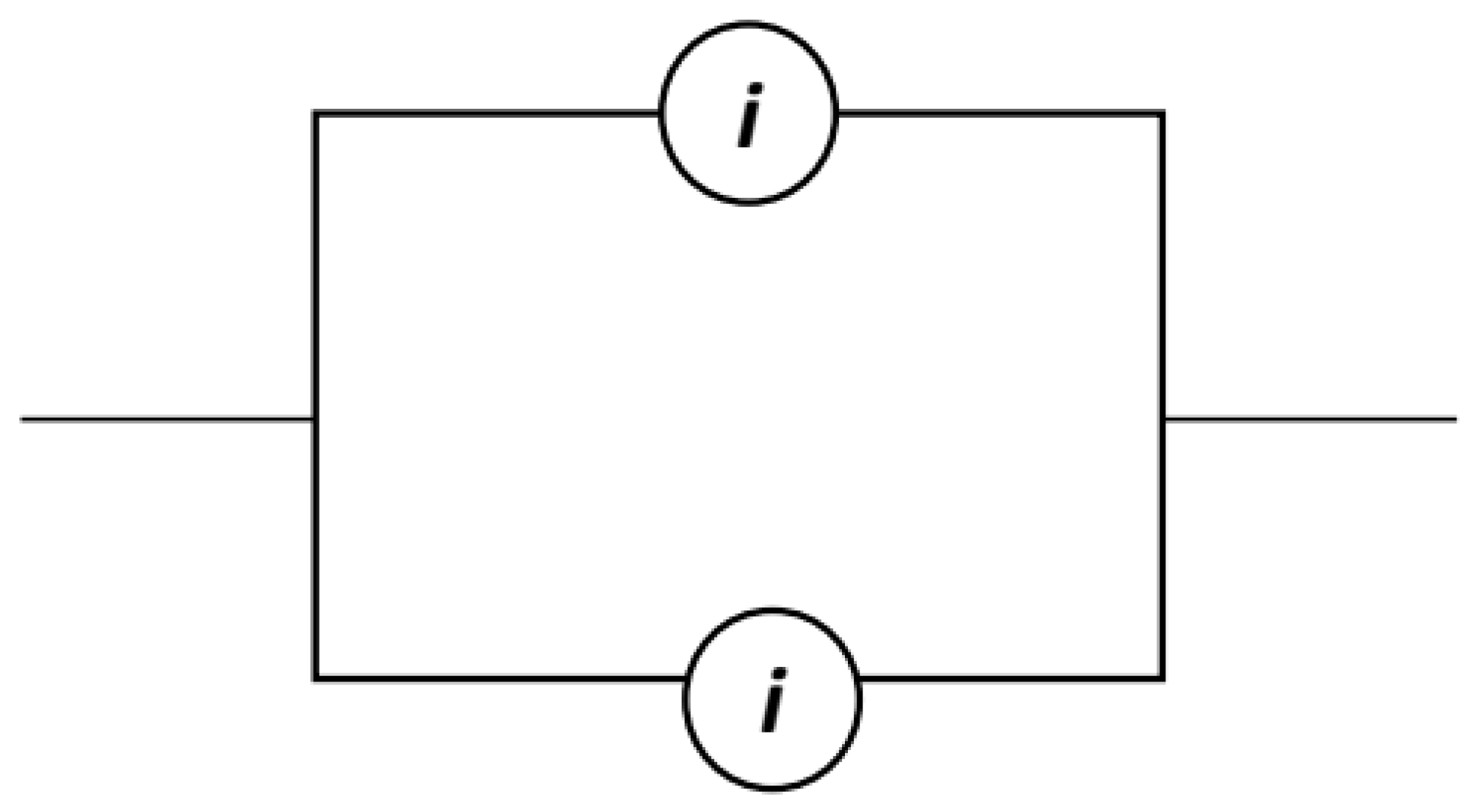
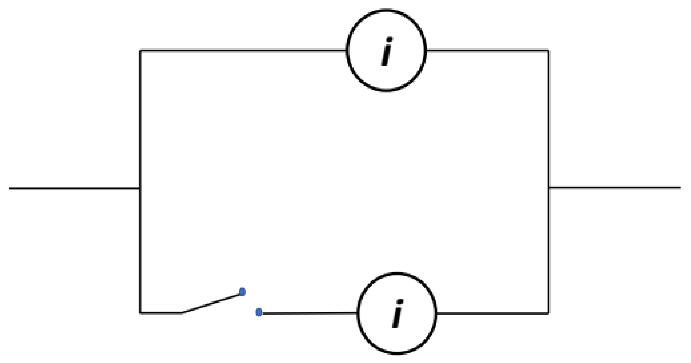
• Components within set B, where $B\in S_i$ for $i=1,\dots ,6$, are enhanced using hot duplication methods. This technique involves adding redundant components that are active simultaneously, thereby improving the overall system reliability.
• Similarly, components in set B are also enhanced using cold duplication methods. In this approach, redundant components are not active until needed, which provides an additional layer of reliability.
• The numerical application involves simulating the performance of the system under various configurations and enhancements. Each configuration is tested to assess how the reduction and duplication methods impact the overall reliability and mean time to failure (MTTF).
• We calculate key reliability metrics, including MTTF and failure probabilities, for each configuration. These metrics help in understanding how each method affects system performance.
• Results of the different methods (reduction, hot duplication, and cold duplication) are compared to highlight the effectiveness of each approach. The comparison includes the assessment of improvements in reliability and performance.
• The assumption of i.i.d.components and the application of GUHLGD are crucial for simplification and analysis and in ensuring uniformity in failure characteristics.
• Each method (reduction, hot duplication, and cold duplication) is applied with careful consideration of its impact on the system’s failure rate and reliability. The numerical results are analyzed to provide a comprehensive understanding of how these methods improve system performance.

The mean time to failure (MTTF) for both the primary and enhanced systems for different values of $\alpha$ and $\beta$ is represented in

Table 1. MTTF for both primary and enhanced systems with $\alpha =3$ and different values of $\theta$.

System	Set	$\mathit{\theta }$
		3	4	5	6	7
Primary	—	0.8199	0.8083	0.8001	0.7943	0.7900
	$S_1$	0.8271	0.8161	0.8083	0.8026	0.7985
	$S_2$	0.8446	0.8351	0.8280	0.8228	0.8188
Hot	$S_3$	0.8514	0.8424	0.8357	0.8307	0.8268
	$S_4$	0.8690	0.8614	0.8554	0.8508	0.8471
	$S_5$	0.8587	0.8503	0.8440	0.8392	0.8355
	$S_6$	0.8763	0.8693	0.8637	0.8593	0.8558
	$S_1$	0.8551	0.8433	0.8127	0.8112	0.8015
	$S_2$	0.8632	0.8511	0.8460	0.8399	0.8034
Cold	$S_3$	0.8539	0.8498	0.8412	0.8395	0.8368
	$S_4$	0.8917	0.8826	0.8707	0.8611	0.8523
	$S_5$	0.8789	0.8698	0.8520	0.8501	0.8482
	$S_6$	0.9311	0.9016	0.8802	0.8679	0.8599

and

Table 2. MTTF for both primary and enhanced systems with $\theta =10$ and different values of $\alpha$.

System	Set	$\mathit{\alpha }$
		3	4	5	6	7
Primary	—	0.7826	0.8413	0.8821	0.9122	0.9349
	$S_1$	0.7911	0.8482	0.8878	0.9167	0.9383
	$S_2$	0.8115	0.8650	0.9016	0.9278	0.9471
Hot	$S_3$	0.8196	0.8716	0.9068	0.9319	0.9502
	$S_4$	0.8401	0.8884	0.9206	0.9431	0.9590
	$S_5$	0.8285	0.8786	0.9123	0.9361	0.9533
	$S_6$	0.8489	0.8954	0.9261	0.9473	0.9621
	$S_1$	0.8131	0.8566	0.9014	0.9437	0.9513
	$S_2$	0.8270	0.8766	0.9211	0.9511	0.9601
Cold	$S_3$	0.8391	0.8812	0.9375	0.9597	0.9712
	$S_4$	0.8611	0.8920	0.9415	0.9608	0.9812
	$S_5$	0.8411	0.8845	0.9219	0.9501	0.9740
	$S_6$	0.8717	0.9180	0.9560	0.9710	0.9991

.

Table 3. $\lambda$ fractiles for primary and enhanced systems with $\alpha =2$ and $\theta =1.5$.

$\mathit{\lambda }$	L	Hot
		${\mathit{S}}_{\mathbf{1}}$	${\mathit{S}}_{\mathbf{2}}$	${\mathit{S}}_{\mathbf{3}}$	${\mathit{S}}_{\mathbf{4}}$	${\mathit{S}}_{\mathbf{5}}$	${\mathit{S}}_{\mathbf{6}}$
0.1	0.8875	0.8926	0.9054	0.9095	0.9182	0.9169	0.9242
0.2	0.8359	0.8440	0.8607	0.8674	0.8794	0.8768	0.8873
0.3	0.7917	0.8021	0.8218	0.8306	0.8456	0.8415	0.8549
0.4	0.7497	0.7618	0.7843	0.7950	0.8129	0.8070	0.8235
0.5	0.7001	0.7205	0.7459	0.7582	0.7794	0.7712	0.7911
0.6	0.6618	0.6761	0.7044	0.7180	0.7431	0.7318	0.7560
0.7	0.6109	0.6255	0.6569	0.6715	0.7015	0.6860	0.7156
0.8	0.5489	0.5628	0.5979	0.6127	0.6497	0.6275	0.6651
0.9	0.4608	0.4723	0.5115	0.5250	0.5736	0.5388	0.5906
$\mathbf{\lambda }$	L	Cold
		${\mathit{S}}_{\mathbf{1}}$	${\mathit{S}}_{\mathbf{2}}$	${\mathit{S}}_{\mathbf{3}}$	${\mathit{S}}_{\mathbf{4}}$	${\mathit{S}}_{\mathbf{5}}$	${\mathit{S}}_{\mathbf{6}}$
0.1	0.8875	0.9066	0.9484	1.2417	0.9765	0.9682	1.1339
0.2	0.8359	0.8598	0.9076	0.9324	0.9526	0.9368	1.1339
0.3	0.7917	0.8183	0.8700	0.8997	0.9278	0.9047	1.1339
0.4	0.7497	0.7780	0.8329	0.8659	0.9017	0.8707	1.1340
0.5	0.7001	0.7363	0.7946	0.8297	0.8734	0.8337	1.0521
0.6	0.6618	0.6911	0.7531	0.7895	0.8422	0.7918	0.9976
0.7	0.6109	0.6394	0.7058	0.7426	0.8063	0.7415	0.9492
0.8	0.5489	0.5753	0.6476	0.6834	0.7627	0.6756	0.8991
0.9	0.4608	0.4824	0.5641	0.5960	0.7035	0.5712	0.8405

illustrates the $\lambda$ fractiles for the primary and enhanced systems with $\alpha =2$ and $\theta =1.5$.

Figure 7 display the reliability functions of the primary and enhanced systems with components enhanced within sets $S_1$, $S_2$, and $S_3$.

Similarly, Figure 8 depict the reliability functions of both primary and enhanced systems with components enhanced within sets $S_4$, $S_5$, and $S_6$.

Additionally, Figure 9 depicts the reliability functions of both primary and enhanced systems using hot and cold duplication methods.

The findings presented in Table 1, Table 2 and Table 3 and Figure 7, Figure 8 and Figure 9 indicate that

• The following inequality holds, demonstrating that cold standby redundancy ($MTT{F}_B^C$) significantly enhances the mean time to failure (MTTF) compared to hot standby redundancy ($MTT{F}_B^H$) and no redundancy: $MTTF<MTT{F}_B^H<MTT{F}_B^C$;
• Inequality $MTTF<MTT{F}_{S_1}^H<MTT{F}_{S_2}^H<MTT{F}_{S_3}^H<MTT{F}_{S_5}^H<MTT{F}_{S_4}^H<MTT{F}_{S_6}^H$ illustrates a consistent improvement in MTTF with increasing levels of hot standby redundancy;
• $MTTF<MTT{F}_{S_1}^C<MTT{F}_{S_2}^C<MTT{F}_{S_3}^C<MTT{F}_{S_5}^C<MTT{F}_{S_4}^C<MTT{F}_{S_6}^C$ indicates a greater enhancement in MTTF with increasing levels of cold standby redundancy;
• As the $\beta$ parameter increases, the MTTF decreases, suggesting an inverse relationship between $\beta$ and system reliability;
• Conversely, an increase in the $\alpha$ parameter leads to a rise in MTTF, indicating a direct relationship between $\alpha$ and system reliability;
• Reliability comparisons ($R<R_{S_1}^D<R_{S_2}^D<R_{S_3}^D<R_{S_5}^D<R_{S_4}^D<R_{S_6}^D$) for both $D=H$ and $D=C$ further highlight that system reliability improves with the addition of standby components;
• For the failure rate, $L\left(\lambda \right)<L_B^H\left(\lambda \right)<L_B^C\left(\lambda \right)$ shows that cold standby redundancy reduces the failure rate more effectively than hot standby redundancy;
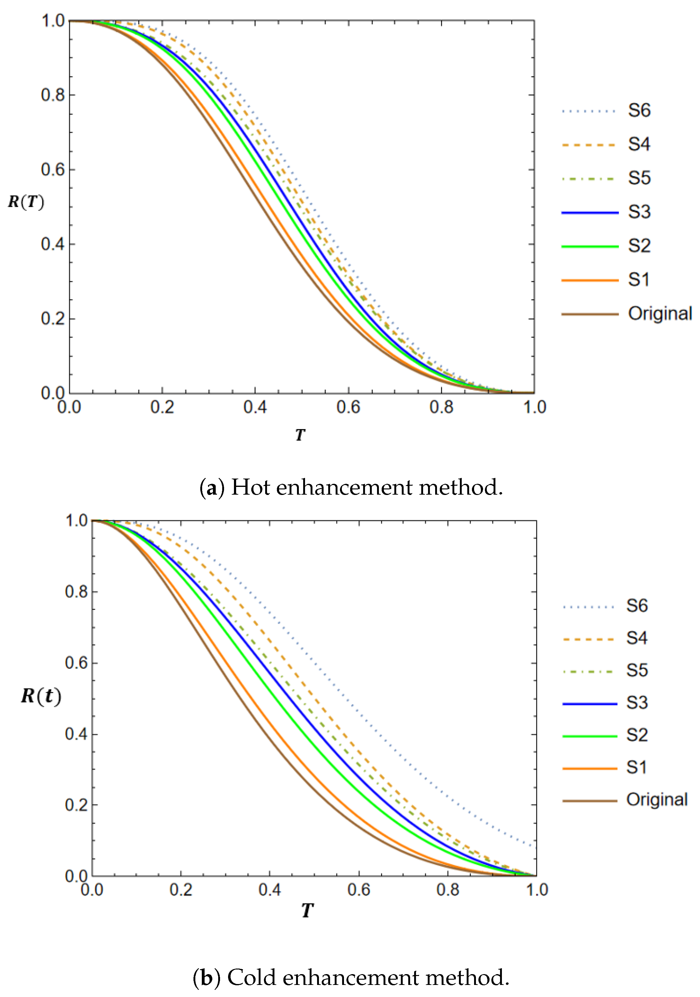
• The most effective method for enhancing the system’s components is the cold duplication technique with a perfect switch, followed by hot duplication, and these methods yield better results than systems without any improvement;
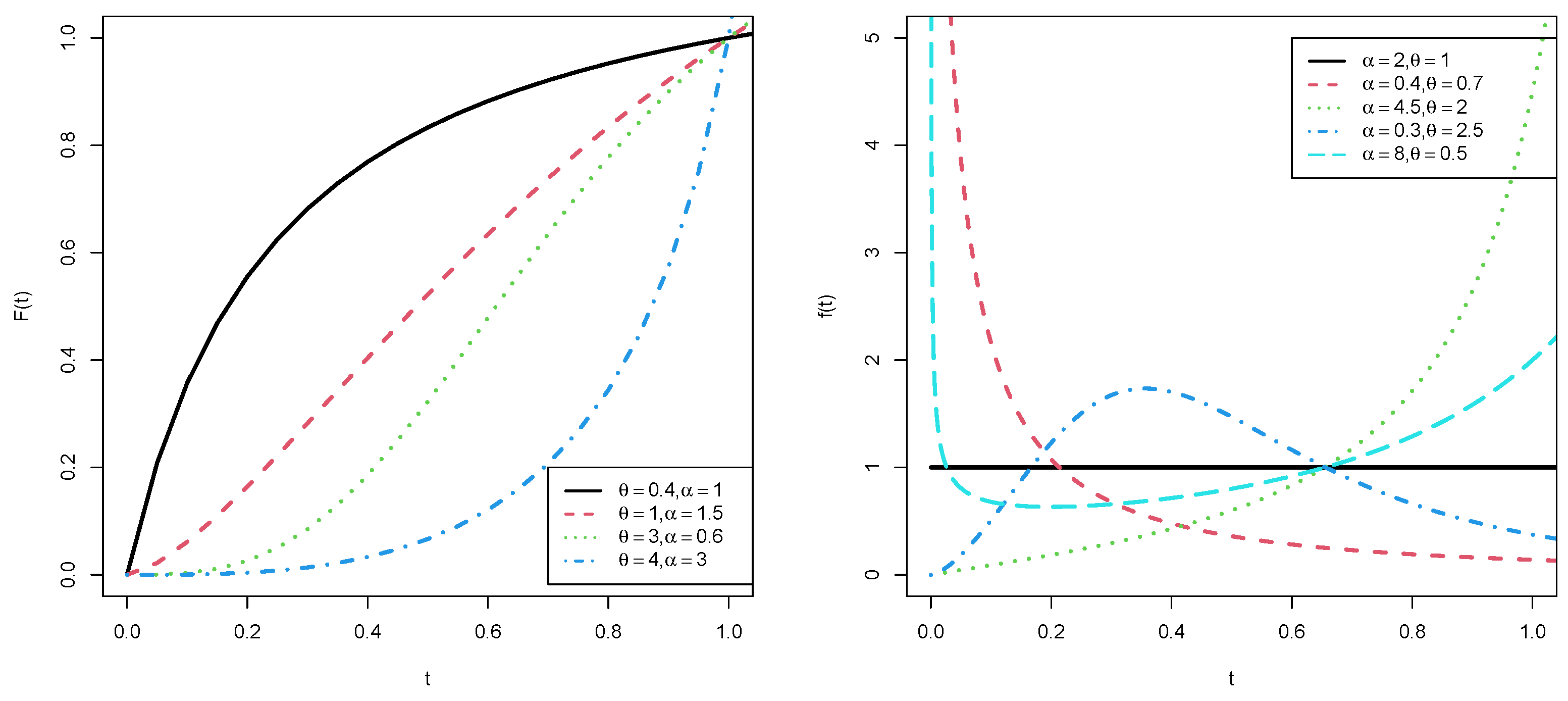
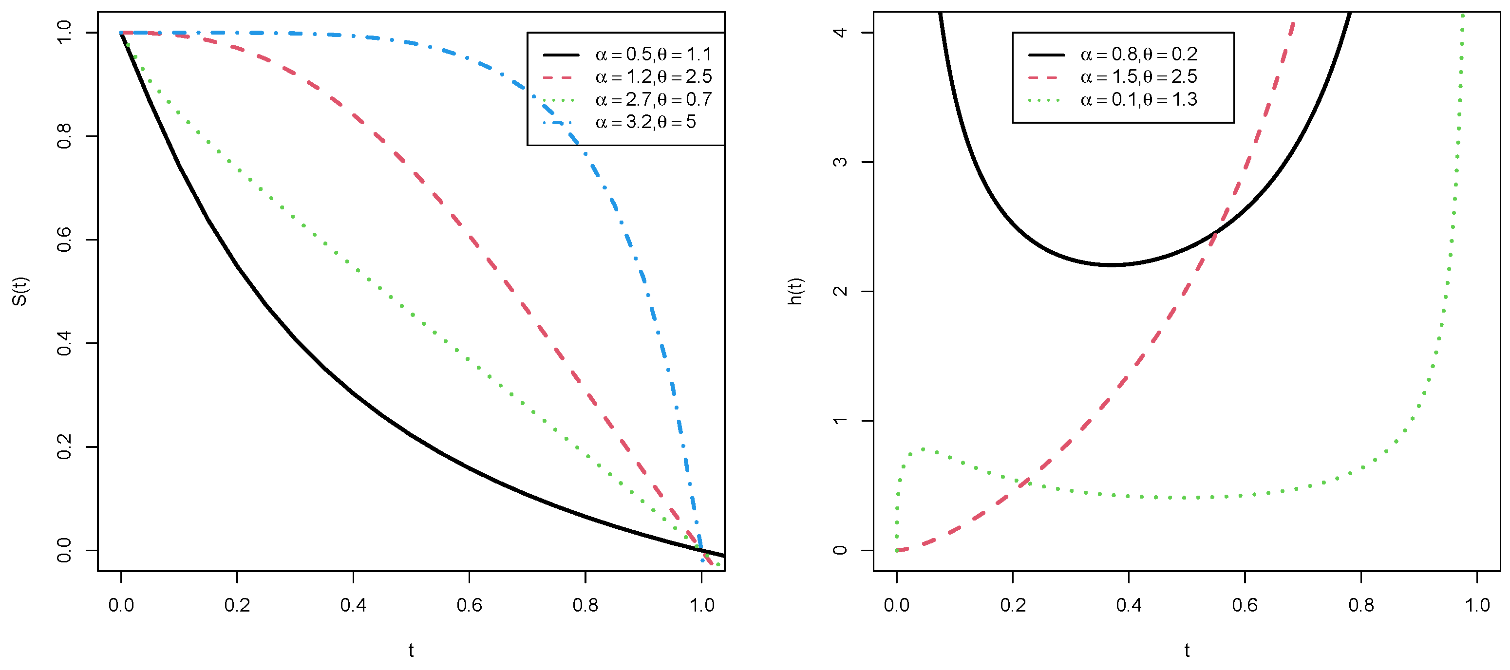
• Numerical results demonstrate that the proposed GUHLGD method provides superior performance in MTTF and reliability compared to traditional methods such as the Bilal, exponential, Weibull, and log-normal distributions. Although Ramadan et al. [17,18] discussed these techniques for improving system reliability using the Bilal distribution, the GUHLGD distribution offers greater flexibility with its probability density function (PDF), which can assume multiple shapes compared to the single shape of the Bilal distribution. This versatility allows the GUHLGD distribution to model a wider range of lifetime data effectively;
• The computational efficiency of the GUHLGD method is comparable to that of traditional methods, ensuring it can be applied to large-scale systems without significant overhead;
• Practical implications of the GUHLGD method include its ability to accurately predict system reliability under various configurations, providing valuable insights for system design and maintenance planning.

The following tables present the values of the REF needed to establish equivalence between the primary system and systems enhanced through hot duplication (see

Table 4. REF values for both the primary and hot-enhanced systems with $\alpha =2$ and $\theta =3$.

$\mathit{\lambda }$	A	Hot, B
		${\mathit{S}}_{\mathbf{1}}$	${\mathit{S}}_{\mathbf{2}}$	${\mathit{S}}_{\mathbf{3}}$	${\mathit{S}}_{\mathbf{4}}$	${\mathit{S}}_{\mathbf{5}}$	${\mathit{S}}_{\mathbf{6}}$
0.1	$S_1$	0.5435	0.2594	0.1352	0.0520	0.0857	0.0483
	$S_2$	0.3761	0.5986	0.1873	0.6430	NA	NA
	$S_3$	0.1519	0.3391	0.4925	NA	NA	NA
	$S_4$	0.8743	0.6584	0.523	NA	NA	0.0170
	$S_5$	0.9124	0.1170	0.4382	NA	0.3761	NA
	$S_6$	0.1204	0.3348	NA	NA	NA	NA
0.3	$S_1$	0.4216	0.2285	0.03575	NA	0.0713	0.0603
	$S_2$	0.4391	0.5872	0.8249	0.1109	NA	NA
	$S_3$	0.7761	0.6350	0.8095	0.8521	NA	NA
	$S_4$	0.7211	0.7443	NA	NA	NA	NA
	$S_5$	0.9285	0.3328	NA	NA	0.6540	0.8929
	$S_6$	0.9972	0.9869	0.2119	0.9301	NA	NA
0.5	$S_1$	0.3321	0.2403	NA	NA	0.1469	0.1661
	$S_2$	0.0982	0.0665	0.1047	0.0984	NA	NA
	$S_3$	0.9591	0.1243	NA	0.8456	0.7986	NA
	$S_4$	0.1626	0.5773	NA	0.9711	0.8312	NA
	$S_5$	0.9220	0.1178	NA	NA	0.9562	0.6682
	$S_6$	NA	0.2030	0.7116	NA	0.5892	NA
0.7	$S_1$	0.2434	0.4101	0.0496	0.1376	0.5544	NA
	$S_2$	NA	NA	0.7051	0.6706	NA	0.9384
	$S_3$	0.4947	NA	0.5800	0.5664	0.4709	0.6409
	$S_4$	0.7592	0.7514	0.8849	0.7092	0.5496	0.9930
	$S_5$	0.9065	0.8271	0.7643	0.7643	0.4896	NA
	$S_6$	0.6898	0.4431	0.7433	NA	NA	0.9064
0.9	$S_1$	0.1300	0.9210	0.6659	NA	NA	NA
	$S_2$	0.7711	0.3865	NA	0.0121	0.6679	NA
	$S_3$	0.8210	NA	NA	0.2776	0.9012	0.1702
	$S_4$	0.4620	0.2815	0.3847	0.3914	0.1780	0.5054
	$S_5$	0.6060	0.5371	0.5653	0.4886	0.4243	NA
	$S_6$	0.8885	NA	NA	NA	NA	0.2572

) and cold duplication (see

Table 5. REF values for both the primary and cold-enhanced systems with $\alpha =2$ and $\theta =1$.

$\mathit{\lambda }$	A	Cold, B
		${\mathit{S}}_{\mathbf{1}}$	${\mathit{S}}_{\mathbf{2}}$	${\mathit{S}}_{\mathbf{3}}$	${\mathit{S}}_{\mathbf{4}}$	${\mathit{S}}_{\mathbf{5}}$	${\mathit{S}}_{\mathbf{6}}$
0.1	$S_1$	0.2476	0.1295	0.4473	0.0658	NA	NA
	$S_2$	0.0946	0.2275	0.1809	NA	NA	NA
	$S_3$	0.9953	0.1129	NA	NA	0.0265	0.3382
	$S_4$	0.8721	0.4486	0.9127	0.0155	0.4437	0.1588
	$S_5$	0.9126	0.3347	0.1762	NA	NA	NA
	$S_6$	0.0170	0.0101	NA	NA	NA	NA
0.3	$S_1$	0.2268	0.2761	0.2863	0.1872	0.5533	0.9126
	$S_2$	0.5887	0.7121	0.3398	0.6578	NA	NA
	$S_3$	0.4473	0.6529	0.8363	NA	NA	NA
	$S_4$	0.1783	0.3387	0.6865	NA	NA	NA
	$S_5$	0.4776	0.2185	0.1101	NA	0.3320	NA
	$S_6$	NA	NA	NA	NA	NA	NA
0.5	$S_1$	0.3329	0.6569	NA	NA	NA	NA
	$S_2$	0.9501	0.1198	0.5438	0.8947	NA	NA
	$S_3$	0.7224	NA	0.0520	NA	0.1147	NA
	$S_4$	0.5112	0.3018	0.3513	0.0308	NA	NA
	$S_5$	0.2374	0.5550	0.3213	NA	NA	NA
	$S_6$	0.6773	0.8639	NA	NA	NA	NA
0.7	$S_1$	0.5531	0.0219	0.9547	NA	NA	NA
	$S_2$	0.4636	0.4737	0.4923	NA	0.3715	NA
	$S_3$	0.3766	0.7852	NA	0.2772	NA	NA
	$S_4$	0.7761	0.7112	NA	NA	NA	0.5546
	$S_5$	0.0334	0.9097	NA	0.3022	NA	NA
	$S_6$	0.8090	0.8707	0.0404	NA	NA	NA
0.9	$S_1$	0.6020	0.5501	0.6280	NA	NA	NA
	$S_2$	0.0015	0.0374	NA	NA	0.5509	NA
	$S_3$	NA	0.1417	NA	NA	NA	NA
	$S_4$	0.6721	0.9804	NA	0.9011	NA	0.0252
	$S_5$	NA	NA	NA	0.553	0.7823	0.9961
	$S_6$	NA	0.5182	0.6590	0.1294	0.0777	NA

) for all enhanced subsets of B.

According to Table 3, Table 4 and Table 5 it is worth noting the following:

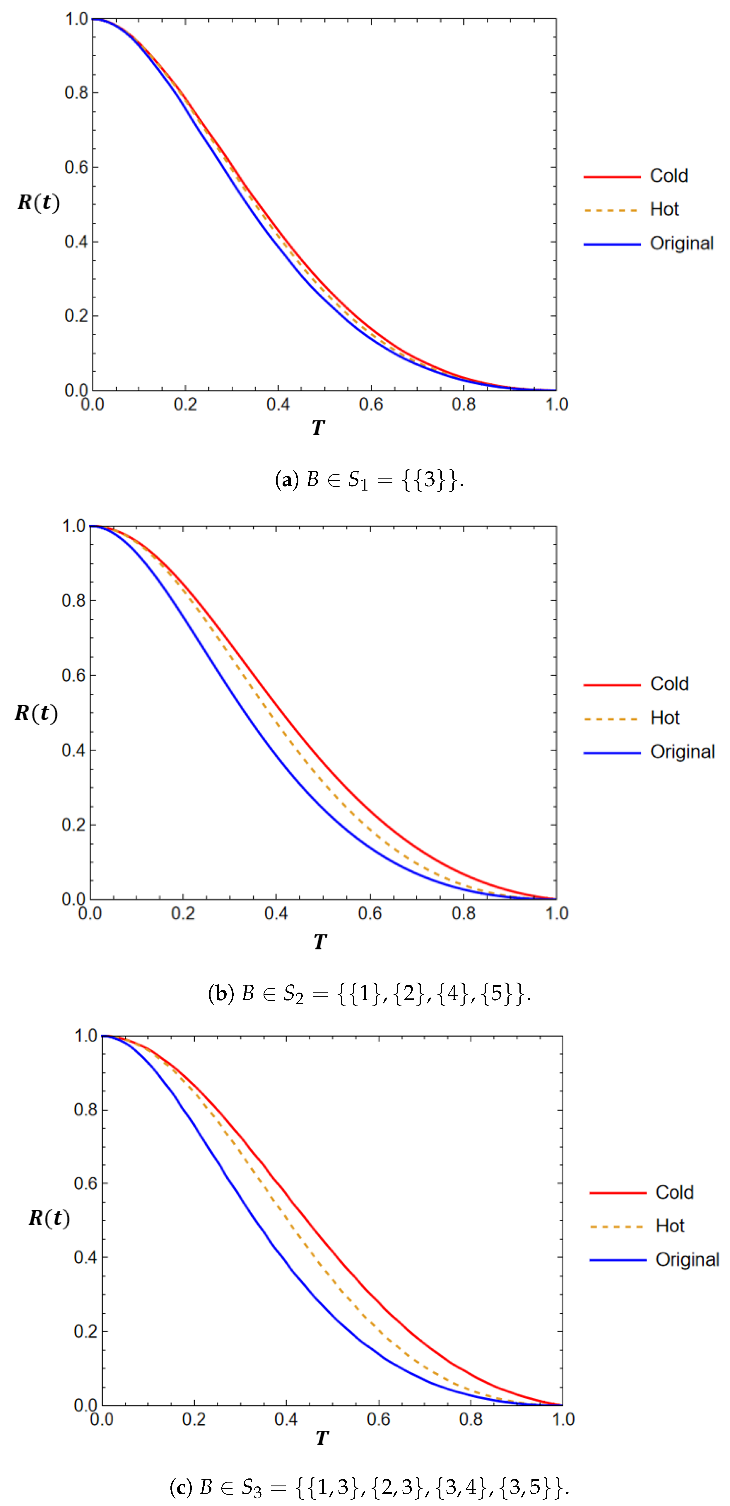
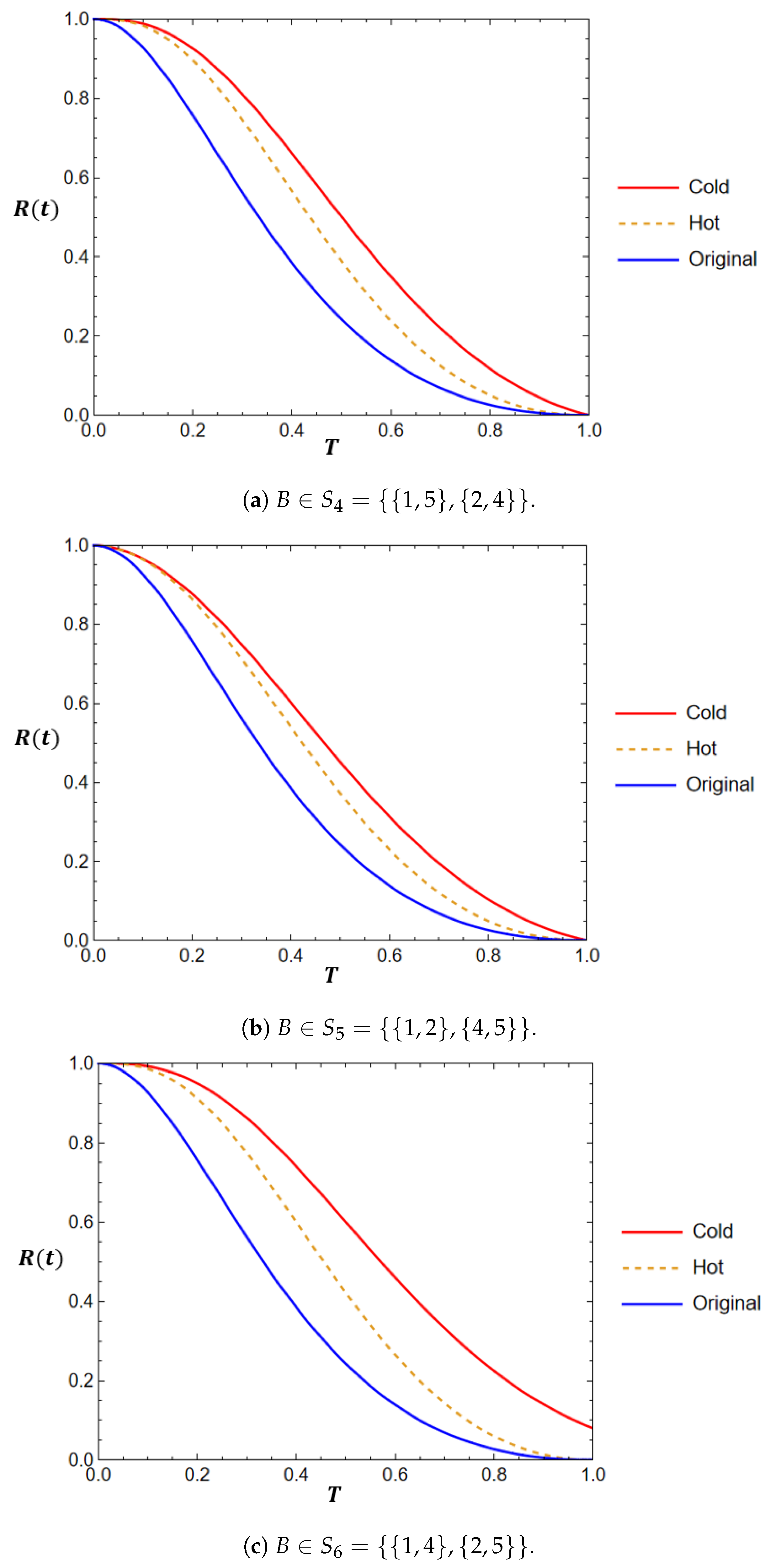
• Table 3 indicates that applying hot duplication to set B within $S_1$ results in an increase of $L\left(0.1\right)$ from $0.8875$ to $0.8926$. This same effect is observed when reducing the failure rates of set A, particularly for the following components: (i) $S_1$ with ${\rho }^H=0.5435$, (ii) $S_2$ with ${\rho }^H=0.2594$, (iii) $S_3$ with ${\rho }^H=0.1352$, (iv) $S_4$ with ${\rho }^H=0.0520$, (v) $S_5$ with ${\rho }^H=0.0857$, and (vi) $S_6$ with ${\rho }^H=0.0483$, as demonstrated in Table 4.
• Additionally, as shown in Table 3, implementing cold duplication for set B within $S_4$ results in an increase of $L\left(0.7\right)$ from $0.6109$ to $0.8063$. This same effect is observed when reducing the failure rates of set A, particularly for the following components: (i) $S_1$ with ${\rho }^C=0.7592$, (ii) $S_2$ with ${\rho }^C=0.7514$, (iii) $S_3$ with ${\rho }^C=0.8849$, (iv) $S_4$ with ${\rho }^C=0.7092$, (v) $S_5$ with ${\rho }^C=0.5496$, and (vi) $S_6$ with ${\rho }^C=0.9930$, as demonstrated in Table 5.
• The abbreviation “NA” signifies that comparing a system enhanced through the reduction method with another system improved through duplication methods is not feasible.

8. Conclusions

In this study, we employed the concept of reliability to examine a bridge system composed of components following the generalized unit half logistic geometric distribution (GUHLGD). We analyzed the following three improvement strategies: reduction, hot duplication, and cold duplication. Our findings highlight several key points. (i) Reduction method: By uniformly reducing the failure rates of components within set A by a factor of $\rho$, we observed a significant improvement in the system’s overall reliability and demonstrated that a targeted reduction in failure rates can effectively enhance the system’s performance. (ii) The hot duplication method: When redundant components within set B are active simultaneously, substantial improvements were also observed. This method ensures that the system maintains functionality, even when primary components fail, thereby increasing the MTTF and overall system reliability. (iii) Cold duplication method: This method involves adding redundant components that remain inactive until needed. It was found to be the most effective among the three strategies. This approach provided the highest reliability and MTTF. The theoretical implications of our findings suggest that incorporating redundancy, whether through hot or cold duplication, is a more effective strategy for enhancing system reliability than merely reducing failure rates. To illustrate these theoretical conclusions, we provided a numerical example demonstrating the application of each method. In conclusion, our study confirms that the use of GUHLGD in modeling component reliability, coupled with strategic enhancements through reduction, hot duplication, and cold duplication, can significantly improve the reliability of bridge systems. The cold duplication method is the most effective approach, providing the highest reliability and MTTF.

9. Future Work

We will improve reliability systems in radar models based on different lifetime distributions and availability equivalence analysis to simulate a repairable bridge network system.

The series-parallel system is one of the important systems in reliability theory and has many applications in engineering sciences. This system has many special use cases, such as in serial, parallel, and radar systems. Therefore, we will study the improvement of the performance of a series-parallel system based on the generalized unit half logistic geometric distribution.

References

1. Lu, Z.H.; Hu, D.Z.; Zhao, Y.G. Second-order fourth-moment method for structural reliability. J. Eng. Mech. 2017, 143, 601–6010. [Google Scholar] [CrossRef]
2. Hasofer, A.M.; Lind, N.C. Exact and invariant second-moment code format. J. Eng. Mech. Div. 1974, 100, 111–121. [Google Scholar] [CrossRef]
3. Zhang, L.W.; Dang, C.; Zhao, Y.G. An efficient method for accessing structural reliability indexes via power transformation family. Reliab. Eng. Syst. Saf. 2023, 233, 109097. [Google Scholar] [CrossRef]
4. Jiang, C.; Qiu, H.; Yang, Z.; Chen, L.; Gao, L.; Li, P. A general failure-pursuing sampling framework for surrogate-based reliability analysis. Reliab. Eng. Syst. Saf. 2019, 183, 47–59. [Google Scholar] [CrossRef]
5. Li, Z.W.; Liu, X.Z.; Chen, S.X. A reliability assessment approach for slab track structure based on vehicle-track dynamics and surrogate model. Proc. Inst. Mech. Eng. Part O J. Risk Reliab. 2022, 236, 79–89. [Google Scholar] [CrossRef]
6. Mustafa, A. Improving the Performance of a Series-Parallel System Based on Gamma Distribution. Int. J. Anal. Appl. 2024, 22, 52. [Google Scholar] [CrossRef]
7. Xu, A.; Fang, G.; Zhuang, L.; Gu, C. A multivariate student-t process model for dependent tail-weighted degradation data. ISE Trans. 2024. [Google Scholar] [CrossRef]
8. Zhuang, L.; Xu, A.; Wang, Y.; Tang, Y. Remaining useful life prediction for two-phase degradation model based on reparameterized inverse Gaussian process. Eur. J. Oper. Res. 2024, 319, 877–890. [Google Scholar] [CrossRef]
9. Alghamdi, S.M.; Percy, D.F. Reliability equivalence factors for a series-parallel system of components with exponentiated Weibull lifetimes. IMA J. Manag. Math. 2017, 28, 339–358. [Google Scholar] [CrossRef]
10. Luo, L.; Xie, X.; Zhang, Y.; He, W. Overview of Calculation Methods of Structural Time-Dependent Reliability. J. Phys. Conf. Ser. 2022, 2148, 12–63. [Google Scholar] [CrossRef]
11. Ezzati, G.; Rasouli, A. Evaluating system reliability using linear-exponential distribution function. Int. J. Adv. Stat. Probab. 2015, 3, 15–24. [Google Scholar] [CrossRef]
12. El-Faheem, A.A.; Mustafa, A.; Abd El-Hafeez, T. Improving the Reliability Performance for Radar System Based on Rayleigh Distribution. Sci. Afr. 2022, 17, e01290. [Google Scholar] [CrossRef]
13. Jaramillo-Vacio, R.; Cruz-Salgado, J.; Ochoa-Zezzatti, A. Selection of Factors Influencing for Reliable Electrical Power Transmission Design in Industry 4.0. Technol. Ind. Appl. Assoc. Ind. 4.0 2022, 4, 217–230. [Google Scholar]
14. Papaioannou, I.; Straub, D. Reliability sensitivity analysis with FORM. In Proceedings of the 13th International Conference on Structural Safety and Reliability (ICOSSAR 2022), Shanghai, China, 13–17 September 2022. [Google Scholar]
15. Peiravi, A.; Karbasian, M.; Ardakan, M.A.; Coit, D.W. Reliability optimization of series-parallel systems with K-mixed redundancy strategy. Reliab. Eng. Syst. Saf. 2019, 183, 17–28. [Google Scholar] [CrossRef]
16. Peyghami, S.; Palensky, P.; Blaabjerg, F. An overview on the reliability of modern power electronic based power systems. IEEE Open J. Power Electron. 2020, 1, 34–50. [Google Scholar] [CrossRef]
17. Ramadan, A.T.; Tolba, A.H.; El-Desouky, B.S. Generalized power Akshaya distribution and its applications. Open J. Model. Simul. 2021, 9, 323–338. [Google Scholar] [CrossRef]
18. Ramadan, A.T.; Tolba, A.H.; El-Desouky, B.S. A unit half-logistic geometric distribution and its application in insurance. Axioms 2022, 11, 676. [Google Scholar] [CrossRef]
19. Xia, T.; Si, G.; Shi, G.; Zhang, K.; Xi, L. Optimal selective maintenance scheduling for series-parallel systems based on energy efficiency optimization. Appl. Energy 2022, 314, 118927. [Google Scholar] [CrossRef]
20. Xia, Y.; Zhang, G. Reliability equivalence factors in gamma distribution. Appl. Math. Comput. 2007, 187, 567–573. [Google Scholar] [CrossRef]
21. Xu, Z.; Saleh, J.H. Machine learning for reliability engineering and safety applications: Review of current status and future opportunities. Reliab. Eng. Syst. Saf. 2021, 211, 107530. [Google Scholar] [CrossRef]
22. Mustaf, A.; El-Desouky, B.S.; Taha, A. Evaluating and improving system reliability of bridge structure using gamma distribution. Int. J. Reliab. Appl. 2016, 17, 121–135. [Google Scholar]
23. Mustaf, A.; El-Desouky, B.S.; Taha, A. Improving the performance of the series-parallel system with linear exponential distribution. Int. Math. Forum 2016, 11, 1037–1052. [Google Scholar] [CrossRef]
24. Mustaf, A.; El-Desouky, B.S.; Taha, A. Reliability equivalence factors of non-identical components series system with mixture failure rates. Int. J. Reliab. Appl. 2009, 10, 43–57. [Google Scholar]
25. Mustaf, A.; El-Desouky, B.S.; Taha, A. Reliability equivalence factors of a system with m non-identical mixed of lifetimes. Am. J. Appl. Sci. 2011, 8, 297. [Google Scholar] [CrossRef]
26. Mustaf, A.; El-Desouky, B.S.; Taha, A. Reliability equivalence factors of a system with mixture of n independent and non-identical lifetimes with delay time. J. Egypt. Math. Soc. 2014, 22, 96–101. [Google Scholar] [CrossRef]
27. Ramadan, A.T.; Alamri, O.A.; Tolba, A.H. Reliability Assessment of Bridge Structure Using Bilal Distribution. Mathematics 2024, 12, 1587. [Google Scholar] [CrossRef]
28. Nasiru, S.; Chesneau, C.; Abubakari, A.G.; Angbing, I.D. Generalized Unit Half-Logistic Geometric Distribution: Properties and Regression with Applications to Insurance. Analytics 2023, 2, 438–462. [Google Scholar] [CrossRef]
29. Breneman, J.E.; Chittaranjan, S.; Elmer, E.L. Introduction to Reliability Engineering; John Wiley & Sons: Hoboken, NJ, USA, 2022. [Google Scholar]
30. El-Damcese, M.A.; Ayoub, D.S. Reliability equivalence factors of a parallel system in two-dimensional distribution. J. Reliab. Stat. Stud. 2011, 4, 33–42. [Google Scholar]
31. Sarhan, A. Reliability equivalence factor of a bridge network system. Int. J. Reliab. Appl. 2004, 5, 81–103. [Google Scholar]
32. Sarhan, A.M.; Mustafa, A. Reliability equivalences of a series system consists of n independent and non-identical components. Int. J. Reliab. Appl. 2006, 7, 111–125. [Google Scholar]
33. Sarhan, A.M. Reliability equivalence factors of a general series–parallel system. Reliab. Eng. Syst. Saf. 2009, 94, 229–236. [Google Scholar] [CrossRef]
34. Sarhan, A.M. Reliability equivalence factors of a parallel system. Reliab. Eng. Syst. Saf. 2005, 87, 405–411. [Google Scholar] [CrossRef]
35. Sarhan, A.M. Reliability equivalence of independent and non-identical components series systems. Reliab. Eng. Syst. Saf. 2000, 67, 293–300. [Google Scholar] [CrossRef]
36. Sarhan, A.M. Reliability equivalence with a basic series-parallel system. Appl. Math. Comput. 2002, 132, 115–133. [Google Scholar] [CrossRef]
37. Baaqeel, H.; Ramadan, A.T.; El-Desouky, B.S.; Tolba, A.H. Evaluating the System Reliability of the Bridge Structure Using the Unit Half-Logistic Geometric Distribution. Sci. Afr. 2023, 21, e01750. [Google Scholar] [CrossRef]
Figure 1. A bridge infrastructure management system.
Mathematics 12 03072 g001
Figure 2. The cdf (left) and the pdf (right) of the GUHLGD across different α and θ values.
Mathematics 12 03072 g002
Figure 3. The survival (left) and hazard (right) functions of the GUHLGD for various θ and α values.
Mathematics 12 03072 g003
Figure 4. Minimal pathways within the bridge system.
Mathematics 12 03072 g004
Figure 5. Component i hot duplication.
Mathematics 12 03072 g005
Figure 6. Component i in a cold redundancy configuration with a flawless switch.
Mathematics 12 03072 g006
Figure 7. Reliability function of primary and enhanced systems when enhancing the components within sets S 1 , S 2 , and S 3 .
Mathematics 12 03072 g007
Figure 8. Reliability function of primary and enhanced systems when enhancing the components within sets S 4 , S 5 , and S 6 .
Mathematics 12 03072 g008
Figure 9. Reliability functions of primary and enhanced systems.
Mathematics 12 03072 g009