Co-Secure Domination in Jump Graphs for Enhanced Security

Abstract

This study proposes a general approach to protect graphs using co-secure domination within jump graphs. In the context of graphs, a dominating set is a group of vertices that are either directly linked or connected to all other vertices within the graph. The minimum cardinality of the dominating set in a graph G is called the domination number $\gamma \left(G\right)$. A set $S\subseteq V$ of a graph G is called a co-secure dominating set, if, for all $u\in S,$ there exists a node $v\in N\left(u\right)$ and in $V\setminus S$ so that $(S\setminus \{u\left\}\right)\cup \left\{v\right\}$ dominates the graph G. ${\gamma }_{cs}\left(G\right)$, the co-secure domination number, is the cardinality of a co-secure dominating set with minimum vertices within the graph G. It is a notable protective strategy in which the nodes that are attacked or damaged in an interconnection network can be replaced with alternative nodes to ensure network security. In a jump graph $J\left(G\right)$, the vertices are the edges of G and the adjacency of the vertices of $J\left(G\right)$ are given by the condition that these edges are not adjacent in G. This paper explains how $\gamma \left(G\right)$ and ${\gamma }_{cs}\left(J\left(G\right)\right)$ are related for the jump graph of various graph classes. The study further determines the exact value for ${\gamma }_{cs}\left(J\left(G\right)\right)$ of specific standard graphs. Additionally, the study characterizes ${\gamma }_{cs}\left(J\left(G\right)\right)=2$ and a tight bond is identified for ${\gamma }_{cs}\left(J\left(G\right)\right)$, particularly for G with specific conditions.

1. Introduction

Graph theory provides a framework for modeling interconnection networks as simple graph $G=(V,E)$. We denote cardinality of a vertex set as $|V|=n$ and the cardinality of the edges as $|E|=m$ in $G$. In interconnection networks, the network components such as computers, routers, and nodes are represented as vertices while the connections or communication links between them as the edges of the graph. This representation facilitates the analysis and implementation of security strategies within interconnection networks [1,2]. It aids in identifying critical nodes, assessing network vulnerabilities, designing redundant backup nodes for critical elements, implementing intrusion detection systems, and mitigating potential threats or attacks.

Domination in graphs plays a vital role in protecting interconnection networks. A set $D\subseteq V$ of G is a dominating set (DS), if every vertex in V is either in D or is directly linked to at least one vertex in D [3]. The strategical placement of mobile guards at particular vertices of the network secures an interconnection network from a variety of attacks and that set of guards forms a dominating set. The smallest number of guards needed to protect the entire network is the domination number (DN), and it is denoted by $\gamma \left(G\right)$. To enhance network resilience against node failures or attacks, various domination variants have emerged [4]. Co-secure domination (CSD) is one such variant that provides an additional layer of protection to the network by allowing the replacement of attacked or damaged nodes with an alternative one without affecting the criterion for dominating set [5]. The co-secure domination number (CSDN) ${\gamma }_{cs}\left(G\right)$ is the minimum number of guards required to secure the network by providing backup mobile guards. The historical basis of the concept of graph protection as well as various strategies for optimizing the existing models are described in [4,5,6]. A characterization of Mycielski graphs with ${\gamma }_{cs}\left(G\right)$ = 2 and 3 is given in [7,8]. An iterative formula for calculating the CSDN of Sierpinski networks is given in [9].

The essential graph concepts utilized in this paper are outlined below. For additional explanations on these basic concepts and key results related to domination, please refer to [3]. The degree of a vertex $v\in G$, denoted by $degv$, signifies the number of edges incident with v in a graph G. The maximum number of edges incidents with a vertex in G is $\Delta \left(G\right)$ and the minimum number of edges incidents with a vertex is denoted by $\delta \left(G\right)$. The open neighborhood of a vertex v is defined as $N\left(v\right)=\{u\in V:uv\in E\}$ and its closed neighborhood is denoted by $N\left[v\right]$, which is the set $N\left(v\right)\cup \left\{v\right\}$. The number of neighbors of an edge $e=uv$ is called the $edge degree$$d\left(e\right)$, where $d\left(e\right)=|N(u)\cup N(v)|-2$. Let $T\subseteq V$ and $v\in T$; if $N\left(u\right)\cap T=\left\{v\right\}$, then u is a T- external private neighbor (epn) of v. The set of all T-epns of v is represented by $EPN(v,T)$ [5]. For all the vertices $u\in V,Max\left\{d\right(u,v):v\in V\}$ is the $eccentricity$ of u and the maximum eccentricity is the $diameter$ of the graph denoted by $diam\left(G\right)$. That is, $diam\left(G\right)=Max\left\{e\right(u):u\in V\}$. The circumference of a graph is defined as the length of the longest cycle, denoted as $c\left(G\right)$.

Various symbols are used to denote distinct graph classes. The path graph is represented as $P_n$, the cycle graph as $C_n$, and the complete graph as $K_n$, where n indicates the number of vertices. Additionally, $K_{m,n}$ denotes the complete bipartite graph with two sets, one containing m vertices and the other containing n vertices, and $K_{1,n}$ denotes the star graph. The Cartesian product of two graphs $G=\left(V\right(G),E(G\left)\right)$, and $H=\left(V\right(H),E(H\left)\right)$, denoted by $G\square H$, is the graph with the vertex set $V\left(G\right)\times V\left(H\right)$, and any two vertices $(u,v),(u^{\prime },v^{\prime })$ are adjacent if and only if either $u=u^{\prime }$ and $v{v}^{\prime }\in E\left(H\right)$ or $v=v^{\prime }$ and $u{u}^{\prime }\in E\left(G\right)$. The vertex corona product of G and H is the graph $G\circ H$, obtained by taking one copy of G, called the center graph, $|V(G)|$ copies of H, called the outer graph, and making the $i^{th}$ vertex of G adjacent to every vertex of the $i^{th}$ copy of H, where $1\le i\le |V(G)|$. The vertex corona product is one of the well-known graph products. It has many real time applications in chemistry, computer, and social networks.

Line Graphs and Jump Graphs

The line graph of an undirected graph G is another graph $L\left(G\right)$ in which each edge in G is a vertex in $L\left(G\right)$ [10]. Two vertices in $L\left(G\right)$ are adjacent if the corresponding edges of G are incident, and vice versa. This graph is also called the ’edge graph’ because it focuses on the connections between the edges of the original graph [11,12]. Some observations about the line graph of certain graph classes used in this article are given here [13].

• $L\left(K_{1,n}\right)=K_n$;
• $L\left(C_n\right)=C_n,n\ge 3$;
• $L\left(P_n\right)=P_{n-1},n\ge 3$.

This article examines the CSDN of jump graphs $J\left(G\right)$, which are the complements of edge-independent edge graphs or line graphs [10]. Chartrand et al. [13] presented the concept of the jump graph and the domination number of these graphs was discussed by Maralabhavi et al. [14]. The domination number of the jump graphs $\gamma \left(J\right(G\left)\right)$ was discussed in [14].

Figure 1 illustrates the transformation of G into its $J\left(G\right)$. The edges $\{1,2,3,4,5,6,7,8\}$ of G serve as the vertices of $J\left(G\right)$. It is to be noted that edges that are adjacent in G are not adjacent in $J\left(G\right)$. Bold vertices indicate the dominating vertices. It is clear that all vertices in the original graph and its jump graph are either bold or adjacent to bold vertices.

This paper includes the following observations:

• The determination of the exact values of the CSDN for jump graphs of specific standard graphs;
• The calculation of the CSDN of jump graphs derived from various graphs classes, such as Windmill, Barbell, Sunlet, Helm, and Lict graphs;
• The characterization of jump graphs with a CSDN of 2;
• The establishment of a tight bond for the CSDN of jump graphs;
• An investigation of the relationship between the CSDN of a jump graph and its underlying graph, particularly under specific conditions related to the graph’s circumference and other parameters.

2. CSDN of Jump Graphs

A set $S\subseteq V\left(J\right(G\left)\right)$ of a jump graph $J\left(G\right)$ is called a co-secure dominating set (CSDS) if for every $u\in S$ there exists a vertex $v\in N\left(u\right)$ and in the compliment of S such that $(S\setminus \{u\left\}\right)\cup \left\{v\right\}$ dominates $J\left(G\right)$. The cardinality of the smallest co-secure dominating set is represented by ${\gamma }_{cs}\left(J\left(G\right)\right)$, which is the co-secure domination number (CSDN) of the jump graph. If $J\left(G\right)$ has isolated vertices, then CSDS does not exist.

Preliminary findings and observations about the CSDN of the line graph of $P_n$, $C_n$, and $K_n$ are summarized in [5,15]: ${\gamma }_{cs}(L\left(C_n\right)={\gamma }_{cs}\left(C_n\right)=\lceil {\displaystyle \frac{2n}{5}}\rceil$, ${\gamma }_{cs}\left(L\left(P_n\right)\right)={\gamma }_{cs}\left(P_{n-1}\right)=\lceil {\displaystyle \frac{2n}{5}}\rceil$, and ${\gamma }_{cs}\left(L\left(K_{1,n}\right)\right)={\gamma }_{cs}\left(K_n\right)=1$.

Bounds and Exact Values for CSDN of Jump Graphs

The analysis of ${\gamma }_{cs}\left(J\left(G\right)\right)$ of certain graph families results in the following theorem. It is easy to prove the following two theorems.

Theorem 1.

1. 

${\gamma }_{cs}\left(J\left(P_n\right)\right)=2,n\ge 5.$

2. 

${\gamma }_{cs}\left(J\left(C_n\right)\right)=2,n\ge 5$.

3. 

${\gamma }_{cs}\left(J\left(K_n\right)\right)=3,n\ge 5$.

4. 

If G is a Spider tree or a Lobster tree with $n\ge 5$, ${\gamma }_{cs}\left(J\left(G\right)\right)=2$.

5. 

${\gamma }_{cs}\left(J\left(K_{m,n}\right)\right)=2,$ for all $m\ge 2,n>3.$

6. 

For the Wheel Graph $W_n,n\ge 5,{\gamma }_{cs}\left(J\left(W_n\right)\right)=3.$

A careful analysis of CSDN with the jump graphs of distinct graph classes yielded the following result.

Corollary 1.

For a connected graph G with n vertices, then ${\gamma }_{cs}\left(J\left(G\right)\right)\ge 2$.

3. Characterization of CSDN of Jump Graphs in Various Graph Classes

The jump graphs of certain derived graphs were analyzed for their CSDN, and a characterization of ${\gamma }_{cs}\left(J\left(G\right)\right)=2$ for these derived graphs was conducted. Graph families under consideration are (i) Cartesian product of graphs, (ii) Windmill graphs, (iii) Barbel graphs, (iv) line graphs, (vi) Sunlet graphs, and (vii) Helm graphs.

Theorem 2.

${\gamma }_{cs}\left(J\left(G\right)\right)=2$ if G is any one of the following three graph families:

(i) 

G has no pendant vertices or G is a tree, and $diam\left(G\right)\ge 3.$

(ii) 

It is an Eulerian graph with $n\ge 3.$

Proof. 

Case (i): Suppose G has no pendant vertices and $diam\left(G\right)\ge 3$.

Consider a graph G with n vertices without isolated vertices, $n\ge 4$, m edges and $diam\left(G\right)>3$. Let $u_1,u_2,\dots ,u_n$ be the longest path in G and $e_1=u_1{u}_2,e_2=u_2{u}_3,\dots ,e_{n-1}=u_{n-1}{u}_n$ be the edges in G. By definition, the edges $e_1$, $e_2$, $e_3$, …, $e_{n-1}$ are vertices in $J\left(G\right)$. For the vertices $e_1$ and $e_{n-1}$ in $J\left(G\right)$, $N\left(e_1\right)=\{e_3$, $e_4$, …, $e_{n-1}\}$ and $N\left(e_{n-1}\right)=\{e_1$, $e_2$, $e_3$, $e_4$, …, $e_{n-3}\}$ [13]. Choose a subset $S\subset V\left(J\right(G\left)\right)$, where $S=\{e_1,e_{n-1}\}$. Since all the vertices of $J\left(G\right)$ are either in S or in $N\left(e_1\right)$ or in $N\left(e_{n-1}\right)$, S is a dominating set for $J\left(G\right)$. The vertex $e_1\in S$ can be replaced by the vertex $e_3$ so that the set ($S\setminus \left\{e_1\right\})\cup \left\{e_3\right\}$ is a dominating set of $J\left(G\right)$. The vertex $e_{n-1}\in S$ can be replaced by $e_2$, since the vertex $\left\{e_2\right\}\in N\left(e_{n-1}\right)$, and the set $(S\setminus$ {$e_{n-1}$ }) ∪ {$e_2$} is a dominating set.

Thus, the set $S=\{e_1,e_{n-1}\}$ is a CSDS of $J\left(G\right)$ with cardinality 2. This is the minimum CSDS because removing a vertex from S disrupts the dominating property of the graph. Hence, ${\gamma }_{cs}\left(J\left(G\right)\right)=2$.

Case (ii): For any tree T with $diam\left(T\right)\ge 3.$

Let $u_i{e}_i{u}_j{e}_j\dots ,u_k{e}_k{u}_{k+1}$ be a path of maximum length in the tree T with pendant vertices $u_i$ and $u_{k+1}$ whose supporting edges are $e_i$ and $e_k$, respectively. The edges of T are the vertices in $J\left(T\right)$ and the total number of vertices in $J\left(T\right)=n-1$. Consider the set $S=\{e_i,e_k\}\subset V\left(J\left(T\right)\right)$. Since $N\left[e_i\right]\cap N\left[e_k\right]=\varphi ,$ in $L\left(G\right)$, by definition of jump graphs, $e_i\in N\left[e_k\right]$ and $e_k\in N\left[e_i\right]$. Thus, $N\left[S\right]=V.$ Hence, S is a DS of $J\left(G\right)$ and $|N[S]|\le 2$. There exists a vertex $e_j\in N\left[e_k\right]$ so that $EPN[e_i,S]\subset N\left[e_k\right]$. Thus, the vertex $e_j$ replaces the vertex $e_i\in S$. S is a CSDS since $EPN[e_i,S]\subset N\left[e_j\right]$, and $e_j\in (V\left(J\left(T\right)\right)\setminus S).$ Thus, $|S|\le 2$.

Similarly, $EPN[e_k,S]\subset N\left[e_{k-2}\right]$, where the vertex $e_{k-2}\in (V\left(J\left(T\right)\right)\setminus S).$ Thus $e_{k-2}$ replaces $e_k$ in S. Since a single vertex in S cannot dominate all vertices in $J\left(G\right)$, the minimum cardinality is at least two. Thus, $|S|\ge 2$. Thus, ${\gamma }_{cs}\left(J\left(T\right)\right)=2$, by the above arguments.

Case (iii): Suppose G is an Eulerian graph, $n\ge 3.$

By definition, if G is an Eulerian graph, the graph possesses a closed trail that traverses each edge exactly once. The trail is a closed path with a diameter greater than 3 for $n\ge 4$. Hence, as proved in Case (i) of this theorem, ${\gamma }_{cs}\left(J\left(G\right)\right)=2.$ □

The following theorem identifies specific graph classes in which ${\gamma }_{cs}\left(J\left(G\right)\right)=2=\gamma J\left(G\right)$.

Figure 2 illustrates the cartesian product (c) $P_3\square K_4$ of the graphs (a) $P_3$ and (b) $K_4.$

Theorem 3.

${\gamma }_{cs}\left(J\left(G\right)\right)$ = $\gamma \left(J\right(G\left)\right)=2$ if G is belonging to any one of the following graph families:

(i) 

The cartesian product of graphs—$P_m\square P_n,C_m\square C_n,C_n\square P_m,C_n\square K_n$.

(ii) 

Windmill graph.

(iii) 

Barbell graph.

Proof. 

(i)

Consider the graph $G\square H$, where $G=P_m$ or $C_m$ or $C_n$ and $H=P_n$ or $C_n$ or $P_m$ or $K_n$.

We know that the Cartesian product of $P_m$ and $P_n$ is the grid graph $P_m\square P_n,\forall m,n\in N$, and N is the set of all natural numbers. We take $G_1=P_m\square P_n$. By definition of the Cartesian product of graphs, $G_1$ has $mn$ vertices and $(m-1)n+(n-1)m$ edges. Thus the $J\left(G_1\right)$ has $2mn-(m+n)$ vertices. The edges in $G_1$ can be $e_1,e_2,e_3,\dots ,e_{mn-1},f_1,f_2,f_3,\dots ,f_{mn-1}$, where $E\left(P_m\right)=\{e_1,e_2,e_3,\dots ,e_{mn-1}\}$ and $E\left(P_n\right)=\{f_1,f_2,f_3,\dots ,f_{mn-1}\}$ respectively. Choose a subset $S_1=\{e_1,e_m\}$ of $V\left(J\left(G_1\right)\right)$, where $e_1\notin N\left(e_m\right)$. $S_1$ dominates all the vertices of $J\left(G_1\right)$. The vertex $e_1\in S_1$ can be replaced by $e_3\in N\left(e_1\right).$ Also, the vertex $e_{mn}\in V\left(J\left(G_1\right)\right)$ can be replaced by the vertex $e_{mn-2}\in J\left(G_1\right)$ in $N\left(e_{mn-1}\right).$ Thus, $S_1$ is a CSDS and its cardinality is 2. It is a minimum dominating set since a single vertex cannot dominate $J\left(G_1\right).$ Hence, ${\gamma }_{cs}J\left(G\right)$ = $\gamma J\left(G\right)=2.$

A similar proof can be applied to the graph $G_2=C_m\square C_n,m,n\ge 3.$ Let the edges in $G_2$ be $g_1,g_2,g_3,\dots ,g_{mn},h_1,h_2,h_3,\dots ,h_{mn}$ respectively, where $E\left(C_m\right)=\{g_1,g_2,g_3,\dots ,g_{mn-1}\}$ and $E\left(C_n\right)=\{h_1,h_2,h_3,\dots ,h_{mn-1}\}.$ It is obvious that the set $S_2=\{h_1,h_{mn-1}\}\subseteq V\left(J\left(G\right)\right)$ is a DS of $V\left(J\left(G_2\right)\right)$ and $|S_2|\ge 2$. The vertex $h_1\in V\left(J\left(G_2\right)\right)$ can be replaced by the vertex $g_{mn}\in V\left(J\left(G_2\right)\right)$. Similarly, $h_{mn}\in S_2$ can be replaced by $h_2\in V\left(J\left(G_2\right)\right).$ Removing a single vertex from $S_2$ will violate the definition of the dominating set of $S_2$. Hence $|S_2|=2.$

Thus, $S_2$ can be a DS as well as CSDS with cardinality two.

Similarly, using the above arguments, we can prove that

${\gamma }_{cs}J\left(G_3\right)={\gamma }_{cs}J(C_m\square P_n)$ and ${\gamma }_{cs}J\left(\left(G_4\right)\right)={\gamma }_{cs}\left(J(C_m\square P_n)\right)=2,m,n\ge 3$.

(ii)

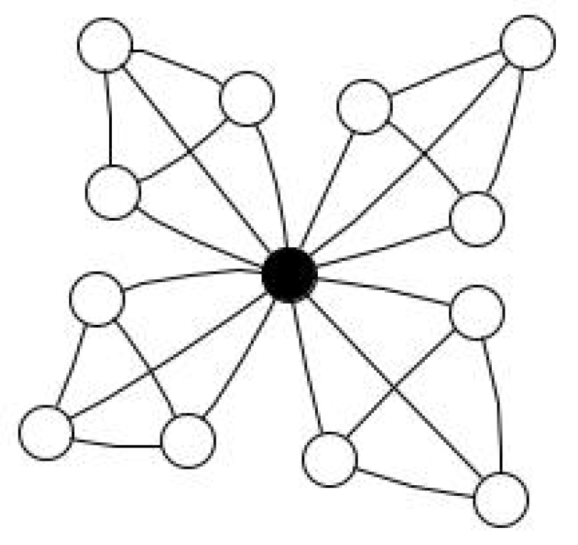
Windmill graph.

Consider a windmill graph $G=W_d[n,m],$ where $n\ge 4,m\ge 2.$ Because all the complete graphs share this universal vertex, the domination number of the windmill graph is $\gamma \left(W_d[n,m]\right)=1.$ The bold vertex in Figure 3 shows this.

Now, consider the jump graph of the windmill graph. Choose any two non-adjacent edges, excluding the edges incident with the universal vertex, to form a DS $S_3=\{e_1,e_2\}.$ Every vertex in $J\left(G\right)$ is dominated by $S_3$. Any non-adjacent edge in $\left(W_d[n,m]\right)$ may replace the vertex $e_1$ in $J\left(\left(W_d[n,m]\right)\right)$, with the exception of the edges incident with the universal vertex in $\left(W_d[n,m]\right)$. In the same way, any non-adjacent edge in $\left(W_d[n,m]\right)$ that is not incident with the edge $e_2$ can be used to substitute the vertex $e_2\in J\left(\left(W_d[n,m]\right)\right)$. This set has cardinality two, making it a CSDS. Furthermore, the required condition for DS is violated when one vertex is removed from $S_3$. Therefore, ${\gamma }_{cs}\left(J\left(G\right)\right)=2=\gamma \left(J\left(G\right)\right)$.

(iii)

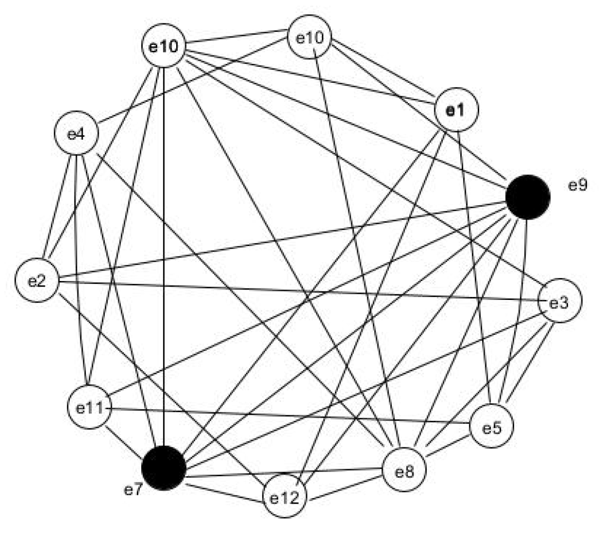
Barbell graph.

We know that in a complete graph with n vertices, $\gamma \left(G\right)={\gamma }_{cs}\left(G\right)=1$. Since two complete graphs are connected by a bridge, two end vertices of the bridge can be taken into the set $S_4=\{u,v\}$, which is clearly a DS. The vertices u and v can be replaced by any x or y$\in K_1$ and $K_2$, and hence $S_4$ is CSDS and hence ${\gamma }_{cs}\left(G\right)=\gamma \left(G\right)=2.$ Create a set $S_6=\{e_1,e_2\}$ by taking two edges that are non-incident with the bridge $e=uv$, where $e_1\in E\left(K_1\right)$ and $e_2\in E\left(K_2\right)$. The edge $e_1$ is adjacent to all edges of $K_2$ and $e_2$ is adjacent to all edges of $K_1$ in $J\left(G\right)$ because every edge in a complete graph is adjacent to every other edge. One of the DS of $J\left(G\right)$ can be taken as $S_6$. The vertex $e_1\in V\left(J\left(G\right)\right)$ can be replaced by any edge of $K_1$ that is not incident with the bridge $e=u v$, and the vertex $e_2$ can be replaced by any edge of $K_2$ that is not incident with the bridge $e=u v$, where $u\in K_1$ and $v\in K_2$. $|S_6|=2$ because removing a single vertex from the set would violate the condition of a dominating set. Hence, ${\gamma }_{cs}\left(J\left(G\right)\right)=\gamma \left(J\left(G\right)\right)=2,$ as a result.

Figure 4 shows an illustration in which a Barbel graph and is its jump graph are given. The edges of the given graph (left figure) become the vertices in the jump graph (right figure) and the edge $e_1$ in the graph is a vertex that is adjacent to $e_3$ and $e_6$ in $J\left(G\right)$. The dominating vertices in the graph G and its jump graph are marked with bold vertices. □

Based on our analysis, it can be demonstrated that for any graph G from the family shown in the Figure 5, we have $\gamma \left(J\left(G\right)\right)={\gamma }_{cs}\left(J\left(G\right)\right)=2$. These graphs have a minimum degree $\delta \left(G\right)\ge 2$ and satisfy $\gamma \left(G\right)={\gamma }_{cs}\left(G\right)=3$.

Corollary 2.

If $G\in \{P_n,C_n,K_n\}$ with $n\ge 5$, then ${\gamma }_{cs}\left(J(G\circ K_m)\right)$ = $\gamma \left(J(G\circ K_m)\right)=2.$

Muddebihal and Kulli introduced the concept of lict graphs in [16]. Lict graphs are the middle graphs of path graphs with $n\ge 4$ [17]. Lict graphs and their corresponding jump graphs were examined for their CSDN. The lict graph is illustrated in Figure 6.

Theorem 4.

For a connected lict graph $L\left(P_n\right)$ with $n⩾4$ and $\delta (L\left(P_n\right)⩾2$, then $\gamma (J\left(L\left(P_n\right)\right)={\gamma }_{cs}(J\left(L\left(P_n\right)\right)=2$.

Proof. 

Consider the given graph as a lict graph $L\left(P_n\right)$ which is the middle graph of the path graph $P_n,n⩾4.$ By definition, $L\left(P_n\right)$ consists of $2n-1$ vertices and $3(n-1)$ edges. The vertex set of $L\left(P_n\right)$ be $V_L=\{u_1,u_2,u_3,\dots ,u_n,u_{1^{\prime }},u_{2^{\prime }},u_{3^{\prime }},\dots ,u_{{(n-1)}^{\prime }}\}$. Consider the sets $S_L\subseteq V_L$, where $S_L$ is defined as $S_L=\{u_1,u_3,u_5,\dots ,u_n\},$ if n is odd and $S_L=\{u_1,u_3,u_5,\dots ,u_{n-1}\}$, if n is even. The set $S_L$ is a dominating set of $L\left(P_n\right)$, since every vertex in ($V_L\setminus S_L)\in N\left(S_L\right)$. $|S_L|\le {\displaystyle \frac{n}{2}}\le \lceil {\displaystyle \frac{n}{3}}\rceil +1.$ Every third vertex in the path graph $P_n$ is in the DS $S_L$. The vertex $u_i\in S_L$ can be replaced by $u_{i^{\prime }}\in \{V_L\setminus S_L\}$ for $i=1,2,3,\dots .,n$, so that the new set $(\{S_L\setminus \left\{u_i\right\})\cup u_{i^{\prime }}\}$ is a DS. Thus, $S_L$ is a CSDS. $|S_L|=\lceil {\displaystyle \frac{n}{3}}\rceil +1$, and by removing a single vertex from the set, $S_L$ is no longer a DS.

Hence, CSDN of lict graph ${\gamma }_{cs}\left(L\left(P_n\right)\right)=\lceil {\displaystyle \frac{n}{3}}\rceil +1.$

Now, consider the jump graph of lict graphs. For all lict graphs $L\left(P_n\right),n\ge 4$, the $diam\left(L\left(P_n\right)\right)>3$ and hence, by Theorem 3, $\gamma (J\left(L\left(Pn\right)\right)={\gamma }_{cs}(J\left(L\left(Pn\right)\right)=2.$ □

Generalisation of CSDN of Jump Graphs

The following theorem provides a generalization of the CSDN for the jump graphs of all connected graphs with a maximum degree $\Delta \left(G\right)\ge 2$ and circumference $c\left(G\right)\ge 4.$

Theorem 5.

For any connected graph G, with $\Delta \left(G\right)\ge 2$ and $c\left(G\right)\ge 4$, $2\le {\gamma }_{cs}\left(J\left(G\right)\right)\le 4.$

Proof. 

It is obvious that ${\gamma }_{cs}\left(J\left(G\right)\right)\ge 2$ for all connected graphs with $\delta \left(G\right)\ge 2$. We divide the graph families based on the diameter.

Case 1:

$diam\left(G\right)=1,c\left(G\right)\ge 4$.

In this class of graphs, since $diam\left(G\right)=1$, every vertex in G is adjacent to every other vertex. Since $c\left(G\right)\ge 4,$ at least two edges in G are non adjacent. Hence, ${\gamma }_{cs}\left(J\left(G\right)\right)\ge 2,$ for $n\ge 4.$ This can be illustrated by taking the cases of any complete graph $K_4$. It is clear that ${\gamma }_{cs}\left(J\left(K_4\right)\right)=3$. Thus, $2\le {\gamma }_{cs}\left(J\left(G\right)\right))\le 4.$

Case 2:

$diam\left(G\right)=2$, $\gamma \left(G\right)=1$, and $c\left(G\right)>4.$

Case 2 (i):

Graphs without pendant vertices.

Clearly, the DS of G will contain u, the vertex with the maximum degree. Take any edge $e_1=v_1{v}_2$ to the DS of $J\left(G\right)$, provided the edge $e_1$ is not incident with the vertex u. Since $\gamma \left(G\right)=1$, the edge $e_1$ is adjacent to all edges in G except the edges that are incident to $e_1$ in G. Let $e_2$ dominate all the edges incident to $e_1$ in G. The set $S_G=\{e_1,e_2\}\subseteq V\left(J\left(G\right)\right)$ is a DS. It is possible to replace $e_1\in J\left(G\right)$ by the vertex $e_3$, where $e_3$ is incident at the vertex $u\in G$. But the set $\{e_3,e_2\}$ cannot dominate all vertices in $J\left(G\right)$. Hence, $S_1\left(G\right)=\{e_1,e_2,e_4\}$, where $e_4$ dominates all the edges incident on the vertex u of G. Thus, $|S_1\left(G\right)|\le 4$.

Case 2 (ii):

Graphs with pendant vertices.

Here, we consider the vertex with a maximum degree in G. Those edges in G that are not incident to the vertex with a maximum degree can enter the DS of $J\left(G\right)$. We consider graphs with a single pendant vertex because an increase in the number of pendant edges increases the $diam\left(G\right)$. As the $c\left(G\right)$ increases, since $\gamma \left(G\right)=1,$ the number of non-incident vertices with a maximum degree vertex is equal to the edges in $c\left(G\right)-2$ + no. of pendant edges in G. The maximum value of DN and CSDN is 4.

Case 3:

Graphs with $diam\left(G\right)=3.$

In this case, we consider the graphs without pendant vertices and with pendant vertices.

Case 3 (i):

Graphs without pendant vertices.

Here, non-adjacent edges to the maximum degree vertex have to be considered. At least three vertices are needed to form a CSDS. Thus, the maximum value of CSDN of $J\left(G\right)$ is 4.

Case 3 (ii):

Graphs with pendant vertices.

In this case, we consider the edges not adjacent or incident to the vertex with a maximum degree in G, including the pendant edges as well. Since $diam\left(G\right)=3$, we can choose at least 3 edges from these sets to dominate $J\left(G\right)$. Consequently, the co-secure domination number is at most $4.$

Case 4:

Graphs with $diam\left(G\right)>3.$

In this case as well, we examine both graphs with and without pendant vertices.

Case 4 (i):

Graphs with $diam\left(G\right)>3$, without pendant vertices.

If G has $diam\left(G\right)>3$, the Theorem 4 provides a thorough explanation that for all connected graphs without pendant vertices, ${\gamma }_{cs}\left(J\left(G\right)\right)=2.$

Case 4 (ii):

Graphs that have $diam\left(G\right)>3$ with pendant vertices.

Consider the helm graph containing 4 pendant vertices, where $c\left(G\right)>4$. Here, the domination number, $\gamma \left(G\right),$ and the CSDN, ${\gamma }_{cs}\left(G\right)$, are 4 and 5, respectively. The pendant edges connected to the principle diagonal edges can be included in the DS of $J\left(G\right),$ leading to $\gamma \left(J\right(G\left)\right)=2.$ The CSDN becomes $2.$ As both the diameter $diam\left(G\right)$ and circumference $c\left(G\right)$ increase, it is observed that ${\gamma }_{cs}\left(J\left(G\right)\right)=2.$

Example: Consider the Helm graph with diameter $4\ge 3$ and pendant vertices in the Figure 7. The jump graph of the same graph is plotted in Figure 8. The dominating vertices are $S_H=\{e_1,e_7\},$ since all other vertices in $J\left(G\right)$ are in $N\left(S_H\right)$.

The pendant vertices will surely enter the DS, and the central vertex will dominate all the other vertices. Thus $\gamma \left(G\right)=5$. All the pendant vertices and the central vertex can be replaced with the supporting vertex, and hence CSDN = 5. When we take the jump graph, since the diameter of the graph is $\ge 3$, by Theorem 2, ${\gamma }_{cs}\left(J\left(G\right)\right)=2$.

□

Corollary 3.

For all graphs G, where G is connected, ${\gamma }_{cs}\left(J\left(G\right)\right)\le {\Delta }_j,$ where ${\Delta }_j$ is the maximum degree of a vertex in $J\left(G\right)$.

Corollary 4.

If four pendant edges are attached to any of the closed graphs say, cycle graph $C_4$, complete graph $K_4$, or wheel graph $W_4$, then the jump graphs of these graphs have, ${\gamma }_{cs}\left(J\left(G\right)\right)=3$.

Theorem 6.

For graphs G with pendant vertices, $k\ge 4$ and circumference $c\left(G\right)\ge 4$, ${\gamma }_{cs}\left(J\left(G\right)\right)\le {\gamma }_{cs}\left(G\right)-1.$

Proof. 

Consider a connected graph G with k pendant vertices and circumference $c\left(G\right)\ge 5.$ It is true that ${\gamma }_{cs}\left(G\right)\ge k$ [5]. Choose a subset $S_j=\{e_i,e_j\}\subset V\left(J\left(G\right)\right)$, where $\{e_i,e_j\}$ are two pendant edges of G that do not share a common edge. Clearly, this set dominates all the vertices of $J\left(G\right)$. Since the two pendant edges of G do not share a common edge and $c\left(G\right)\ge 4$, each vertex in $S_j$ can be replaced by another pendant edge in G, which is in the $N\left(e_i\right)\in V\left(J\left(G\right)\right)$, and hence ${\gamma }_{cs}\left(J\left(G\right)\right)\ge 2$. By theorem $6,$ it is clear that $2\le {\gamma }_{cs}\left(J\left(G\right)\right)\le 4.$ Thus, ${\gamma }_{cs}\left(J\left(G\right)\right)\le {\gamma }_{cs}\left(G\right)-1$, because $k>4$ and ${\gamma }_{cs}\left(G\right)\ge k,$ and ${\gamma }_{cs}\left(J\left(G\right)\right)\le {\gamma }_{cs}\left(G\right)$, when $k=4$. □

We consider the jump graph of Sunlet graphs and Helm graphs [18]. These graphs show $\gamma \left(G\right)={\gamma }_{cs}\left(G\right)=n$ and $\gamma \left(J\left(G\right)\right)={\gamma }_{cs}\left(J\left(G\right)\right)=2$. Analysing the jump graphs of these two graphs for the co-secure domination number, we obtain ${\gamma }_{cs}\left(J\left(G\right)\right)\le {\gamma }_{cs}\left(G\right)-1.$ The result is demonstrated in following figure. The sunlet graph shown in Figure 9 and its jump graph is given in Figure 10. We can see that for a sunlet graph G in the Figure 9, the black vertices are the dominating vertices as well as co-secure dominating vertices. Hence, $\gamma \left(G\right)={\gamma }_{cs}\left(G\right)=5.$ The jump graph in the Figure 9 clearly explains $\gamma \left(J\left(G\right)\right)={\gamma }_{cs}\left(J\left(G\right)\right)=2$, where the CSDS of $J\left(G\right)$ is $\{1,8\}.$

4. Conclusions

This paper examines ${\gamma }_{cs}\left(J\left(G\right)\right)$ across various graph classes and its relationship with other graph parameters. We provide exact values of ${\gamma }_{cs}\left(J\left(G\right)\right)$ for certain standard graphs and characterize jump graphs with ${\gamma }_{cs}\left(J\left(G\right)\right)=2$. Additionally, we establish a tight bond on ${\gamma }_{cs}\left(J\left(G\right)\right)$, particularly for jump graphs derived from other graphs and those with pendant vertices under specified conditions. This method has significant applications in analyzing and implementing security strategies within interconnection networks. In the domain of cyber-security, co-secure domination involves identifying critical nodes where guards should be stationed to maintain network stability. If a guard is compromised or needs to be relocated, another guard must immediately replace them to ensure continuous security. This approach is crucial for protecting network security against attacks or failures. By applying these mathematical concepts, cyber-security professionals can develop more effective defense systems to safeguard critical network infrastructure.

References

- Hsu, L.-H.; Lin, C.-K. Graph Theory and Interconnection Networks; CRC Press: Boca Raton, FL, USA, 2008. [Google Scholar]
- Widmayer, P.; Neyer, G.; Eidenbenz, S. (Eds.) Graph-Theoretic Concepts in Computer Science. In Proceedings of the 25th International Workshop, WG’99, Ascona, Switzerland, 17–19 June 1999; Springer: Berlin/Heidelberg, Germany, 2003. [Google Scholar]
- Haynes, T.W.; Hedetniemi, S.; Slater, P. Fundamentals of Domination in Graphs; CRC Press: Boca Raton, FL, USA, 2013. [Google Scholar]
- Cockayne, E.J.; Grobler, P.J.P.; Grundlingh, W.R.; Munganga, J.; Van Vuuren, J.H. Protection of a graph. Util. Math. 2005, 67, 19–32. [Google Scholar]
- Arumugam, S.; Ebadi, K.; Manrique, M. Co-secure and secure domination in graphs. Util. Math. 2014, 94, 167–182. [Google Scholar]
- Klostermeyer, W.F.; Mynhardt, C.M. Protecting a graph with mobile guards. Appl. Anal. Discret. Math. 2016, 10, 1–29. [Google Scholar] [CrossRef]
- Manjusha, P.; Chithra, M.R. Co-secure domination in Mycielski graphs. J. Comb. Math. Comb. Comput. 2020, 113, 289–297. [Google Scholar]
- Nayana, P.G.; Iyer, R.R. On secure domination number of generalized Mycielskian of some graphs. J. Intell. Fuzzy Syst. Prepr. 2023, 44, 1–11. [Google Scholar] [CrossRef]
- Manjusha, P.; Iyer, R.R. Application of Co-Secure Domination in Sierpinski Networks. In Proceedings of the 2022 IEEE 4th PhD Colloquium on Emerging Domain Innovation and Technology for Society (PhD EDITS), Bangalore, India, 4–5 November 2022. [Google Scholar]
- Basavanagoud, B.; Mathad, V. Graph equations for line graphs, jump graphs, middle graphs, splitting graphs and line splitting graphs. Mapana J. Sci. 2010, 9, 53–61. [Google Scholar] [CrossRef]
- Sastry, D.V.S.; Raju, B.S.P. Graph equations for line graphs, total graphs, middle graphs and quasi-total graphs. Discret. Math. 1984, 48, 113–119. [Google Scholar] [CrossRef]
- Venkatachalapathy, M.; Kokila, K.; Abarna, B. Some trends in line graphs. Adv. Theor. Appl. Math. 2016, 11, 171–178. [Google Scholar]
- Chartrand, G.; Hevia, H.; Jarrett, E.B.; Schultz, M. Subgraph distances in graphs defined by edge transfers. Discret. Math. 1997, 170, 63–79. [Google Scholar] [CrossRef]
- Maralabhavi, Y.B.; Anupama, S.B.; Goudar, V.M. Domination Number of JUMP Graph; Hikari Ltd.: Rousse, Bulgaria, 2013; Volume 8, pp. 753–758. [Google Scholar]
- Beineke, L.W.; Bagga, J.S. Line Graphs and Line Digraphs; Springer: Berlin/Heidelberg, Germany, 1990. [Google Scholar]
- Muddebihal, M.H.; Kulli, V.R. Lict and Litact graph of a graph. J. Anal. Comput. 2006, 3, 33–43. [Google Scholar]
- Basavanagoud, B.; Mathad, V.N. Graph equations for line graphs, jump graphs, middle graphs, litact graphs and lict graphs. Acta Cienc. Indica Math. 2005, 31, 735. [Google Scholar]
- Frucht, R. Graceful numbering of wheels and related graphs. Ann. N. Y. Acad. Sci. 1979, 319, 219–229. [Google Scholar] [CrossRef]
Disclaimer/Publisher’s Note: The statements, opinions and data contained in all publications are solely those of the individual author(s) and contributor(s) and not of MDPI and/or the editor(s). MDPI and/or the editor(s) disclaim responsibility for any injury to people or property resulting from any ideas, methods, instructions or products referred to in the content. |
© 2024 by the authors. Licensee MDPI, Basel, Switzerland. This article is an open access article distributed under the terms and conditions of the Creative Commons Attribution (CC BY) license (https://creativecommons.org/licenses/by/4.0/).
Share and Cite
Pothuvath, M.; Iyer, R.R.; Asiri, A.; Somasundaram, K. Co-Secure Domination in Jump Graphs for Enhanced Security. Mathematics 2024, 12, 3077. https://doi.org/10.3390/math12193077
Pothuvath M, Iyer RR, Asiri A, Somasundaram K. Co-Secure Domination in Jump Graphs for Enhanced Security. Mathematics. 2024; 12(19):3077. https://doi.org/10.3390/math12193077
Chicago/Turabian StylePothuvath, Manjusha, Radha Rajamani Iyer, Ahmad Asiri, and Kanagasabapathi Somasundaram. 2024. "Co-Secure Domination in Jump Graphs for Enhanced Security" Mathematics 12, no. 19: 3077. https://doi.org/10.3390/math12193077