
Closed-Form Performance Analysis of the Inverse Power Lomax Fading Channel Model


Department of Intelligent Radiophysical Information Systems (IRIS), Physics Faculty, P.G. Demidov Yaroslavl State University, Yaroslavl 150003, Russia
Mathematics 2024, 12(19), 3103; https://doi.org/10.3390/math12193103 (registering DOI)
Submission received: 6 September 2024
/
Revised: 27 September 2024
/
Accepted: 30 September 2024
/
Published: 3 October 2024
(This article belongs to the Special Issue Advanced Algorithms in Wireless Communication and Internet of Things (IoT))
Abstract
:This research presents a closed-form mathematical framework for assessing the performance of a wireless communication system in the presence of multipath fading channels with an instantaneous signal-to-noise ratio (SNR) subjected to the inverse power Lomax (IPL) distribution. It is demonstrated that depending on the channel parameters, such a model can describe both severe and light fading covering most cases of the well-renowned simplified models (i.e., Rayleigh, Rice, Nakagami-m, Hoyt, , Lomax, etc.). This study provides the exact results for a basic statistical description of an IPL channel, including the PDF, CDF, MGF, and raw moments. The derived representation was further used to assess the performance of a communication link. For this purpose, the exact expression and their high signal-to-noise ratio (SNR) asymptotics were derived for the amount of fading (AoF), outage probability (OP), average bit error rate (ABER), and ergodic capacity (EC). The closed-form and numerical hyper-Rayleigh analysis of the IPL channel is performed, identifying the boundaries of weak, strong, and full hyper-Rayleigh regimes (HRRs). An in-depth analysis of the system performance was carried out for all possible fading channel parameters’ values. The practical applicability of the channel model was supported by comparing it with real-world experimental results. The derived expressions were tested against a numerical analysis and statistical simulation and demonstrated a high correspondence.
Keywords:
fading channel; statistical description; inverse power Lomax; error rate; outage; capacityPACS:
89.70.+c; 84.40.UaMSC:
94A15; 94A401. Introduction
Wireless communications channels’ statistical description is a mature field of science and engineering that has significantly evolved during the last two decades [1,2,3]. This is mainly due to the rapid evolution of communication networks and systems and the necessity of high-quality predictions of their performance [4,5,6]. It is particularly relevant for tasks related to the analysis of ad hoc communication systems, including 5G NR [7], 6G [8], V2X [9], Wi-Fi 7 [10], Wi-Fi 8 and beyond [11], and unmanned aerial vehicle (UAV) systems [12,13], which greatly suffer from wireless link degradation. Although a wide range of measurement campaigns has been conducted [13,14,15,16,17,18,19], the thickening of propagation conditions prevents the possible unification and generalization of its statistical description.
An extensive growth in the number of proposed models started with the outstanding works by M.D. Yacoub and colleagues [20,21,22,23,24] and continues to the present day with a wide range of various types, including the most intricate ones [25] and the most simplistic [26,27]. Although these models cover a wide range of practical channels, much effort has been put into modeling heavy fading, which corresponds to poor propagation conditions. Such scenarios are generally covered by the so-called heavy-tailed distributions, with one of the most recent examples being the Lomax channel [26]. Notably, the authors in [26] specifically focused on the most simplistic model, but the Lomax distribution has many modifications (suitable for wireless communications) that combine both flexibility and analytical tractability. Among such modifications, one can mention the inverse power Lomax.
The inverse power Lomax distribution (first proposed in [28]) is a three-parametric distribution family and was addressed for a wide range of applications related to econometrics (e.g., GDP analysis [29]), survey sampling, biological sciences (e.g., biological survival data [30]), engineering sciences (e.g., failure times for repairable items [31]), medical research (e.g., relief times analysis [28]), testing problems [32], and social and environmental sciences (e.g., school education-related problems [33] and flood discharges [34]). Moreover, the specific focus of [28] was on applications where censored data arise (with Type-I and Type-II censoring). Furthermore, it was numerously generalized, yielding more complex models, including the four-parametric model, the so-called modified alpha power transformation-inverse power Lomax [33], and the Type-II Topp–Leone modification for the IPL [35]. In spite of being widely used in various applications, its usage in communication systems design, and specifically in wireless communications, is absent.
Recently, a simplified subcase of the IPL, i.e., the classical Lomax model [36], was proposed to describe the statistical effects of a fading wireless communication channel [26]. In their research, Sanchez and López-Martínez [26] aimed to derive a simplified model capable of handling practically valuable scenarios while at the same time being analytically tractable in closed form without resorting to complex functions. It was demonstrated that all the basic statistical characteristics required for a system performance analysis (i.e., the probability density function (PDF), the cumulative distribution function (CDF) and its inverse (ICDF), its raw moments, the moment-generating function (MGF), and its generalization (GMGF)) can be expressed in closed form in contrast to some classical fading distributions (e.g., Rician, Nakagami-m, and Hoyt distributions) [26]. While defining the term “closed-form”, the authors state that “We take the usual convention in the literature, which considers a closed-form as that including a finite number of well-known functions [26]. This classically includes special functions like Bessel or Hypergeometric ones, but not more involved ones like Meijer-G or Fox-H functions”. Although the rigor and clarity of the presented results are praiseworthy, the practical aspects of the chosen approach can be argued. For example, the results in [37] (i.e., [26]) are delivered in terms of various bivariate confluent hypergeometric functions, which are nonstandard for most modern computer algebra systems (CASs) (although they can be easily implemented via series summation or numerical integration). In contrast, the classical univariate Meijer-G or Fox-H functions are implemented in most CASs and have the same computational complexity as the ones mentioned above. Nevertheless, [26] presented not only the statistical description but also most of the Lomax channel-performance metrics (the average bit error rate (ABER), ergodic capacity (EC), and outage probability (OP)). The model was further used for a spectrum sensing analysis [38,39]. One of its key properties, as mentioned in [26,39], is that it is always in the hyper-Rayleigh regime (HRR) (at least the weak HRR) and thus can describe heavy fading conditions, which are of paramount importance for modern urban wireless communications. This can be linked to the fact that the Lomax family (with its modifications) belongs to the heavy-tailed distributions [28], which tend to describe poor propagation conditions.
Additionally, in the last few years, the performance of modern wireless communications has been successfully described with the help of the inverse distributions approach (e.g., inverse gamma shadowing models [40] or inverse Gaussian and inverse generalized Gaussian models [41]) and their power-transformed modifications [42,43,44,45]. Hence, the inverse power Lomax model incorporates all these approaches.
Although much effort has been applied to the description of the IPL model in various applications (from economics to social sciences), it has not been studied in communication theory.
Thus, motivated by the problem stated above, this research studies the performance of a wireless communications system functioning in the presence of a multipath fading channel with the instantaneous signal-to-noise ratio (SNR) subjected to the inverse power Lomax distribution.
The major contributions of this research can be summarized as follows:
- An easy-to-use statistical formulation (in terms of the PDF and CDF) of the inverse power Lomax fading channel model is introduced.
- A specific positioning of the IPL model among the ones most widely used in wireless communications is performed. The results help to identify its capability to handle both severe and light fading, depending on the channel parameters.
- The closed-form expressions are derived for (a) the moment-generating function of the instantaneous SNR; (b) amount of fading (AoF); (c) outage probability (OP); (d) average bit error rate (ABER); and (e) ergodic channel capacity (EC).
- Closed-form high-SNR asymptotic expressions for all the derived channel-performance metrics are derived.
- The closed-form and numerical hyper-Rayleigh analysis of the IPL channel is performed, identifying the boundaries of weak, strong, and full hyper-Rayleigh regimes.
- A thorough joint analysis of the dependence of all the assumed channel-performance metrics on the channel parameters is performed for different fading scenarios—heavy fading and light fading.
- The numerical and statistical simulation results are presented, proving the correctness of the performed theoretical analysis.
- The practical applicability of the proposed model was verified using a variety of datasets, including both synthetic computer-generated data and real-world experimental measurements.
The remainder of this paper is organized as follows: Section 2 provides some preliminary information about the underlying IPL model and derives its representation (in terms of the PDF and CDF), suitable for communications systems’ descriptions, as well as its MGF with its high-SNR asymptotics; Section 3 derives the results for the specific application of the IPL channel in wireless communications (i.e., the exact expressions for the AoF, ABER, OP, and EC); Section 4 delivers an in-depth analysis (theoretical, numerical, and simulation) of the derived expressions for all specific channel and system parameters’ values; and conclusions are drawn in Section 5.
2. IPL Channel Statistical Description
2.1. PDF and CDF of the Instantaneous SNR
This research considers that the instantaneous SNR follows the inverse power Lomax distribution with the PDF and CDF defined as follows [28]:
which are valid for arbitrary positive-distribution parameters (i.e., the scale parameter and the shape parameters and ).
Although such a model can be used for further elaborations, it is conventional to perform a reparametrization in terms of the average SNR as given by the following Lemma:
Lemma 1.
The random variable γ is assumed to follow the two-parametric inverse power Lomax model (i.e., ) with the average value and channel parameters if its PDF and CDF admit the following representation:
Proof of Lemma 1.
To perform this step, one needs the expression for the moments of the instantaneous SNR, i.e., (where r is the order of the moment and is the expectation operator).
Starting from the definition and performing the change in variable , after some straightforward manipulations, yields
where is the Euler gamma function [46].
It must be pointed out that (4c) is valid for any positive and but for , which implies a new restriction on , when evaluating the moments of .
Calculating the average SNR, i.e., , and evaluating leads to
where is introduced for notation clarity in the following way:
For further analysis, one resorts to as a “power-transformation parameter” and as a “shape parameter” of the distribution.
It must be pointed out that the form (3) is quite similar to the corresponding expression for the model (see [42]); thus, some explanations are needed. At its core, the difference between the two lies in the way they are derived: to derive the instantaneous SNR statistics, [42] assumes the -transformed signal’s envelope, which experiences inverse Nakagami-m shadowing. In contrast, here, the -transformed inverse of the SNR is assumed. Moreover, it can be demonstrated that the models cannot be derived from one another by reparameterization. For example, the closest match can be achieved when in [42] is set to one, but this is not allowed for the shadowing model assumed in [42] (i.e., ).
2.2. MGF of the Instantaneous SNR
Theorem 1.
The moment-generating function of the IPL channel and its high-SNR asymptotics are given by
Proof of Theorem 1.
where the equality (10c) is obtained via the transformation of variable :
where is the Fox H-function [46], (11a) is due to () from [51], and (11b) and (11c) are derived with the help of ()–() from [51]:
Combining (10c) with (11c) and (12) and using the power-transformation property of the Fox H-function (see () in [51]), the expression for the moment-generating function can be expressed as
To obtain a high-SNR asymptotic expression for (14b), one can resort to [53] (see expression (3) and (4) in [53]). In this case, one obtains
where and are defined in [53] (see expression (3) and (4), respectively). For the IPL model, and , which finally helps to derive the high-SNR asymptotics for the MGF of the IPL model as
□
It must be noted that the univariate Fox H-functions are implemented in most modern computer algebra systems (e.g., Wolfram Mathematica, MATLAB, Maple, etc.). Thus, (14b) can be easily computed for arbitrary channel parameters, although the computational time can vary, and for some values of and , evaluations can be time-consuming. To speed up the computations, the integral representation of the Fox H-function can be implemented, and efficient numerical integration strategies can be employed. In this case, the MGF (14b) can be rewritten in the following form:
where is the contour chosen in such a way as to separate the poles of the gamma function with opposite signs for the integration variable. For instance, it can be chosen as .
3. IPL Fading Channel Model Application
The derived expressions for the PDF, CDF, and MGF provide a complete first-order statistical representation for assessing the performance of a wireless communication system operating under fading conditions. According to the general framework, communication link reliability is typically quantified in terms of the outage probability, while link quality is measured by the average error rate and ergodic capacity. The impact of fading is conventionally described by the amount of fading and the hyper-Rayleigh regimes.
3.1. Amount of Fading
The amount of fading is defined as the variance of the instantaneous SNR normalized by its squared average value:
Theorem 2.
The amount of fading () for the IPL channel model is given by
Proof of Theorem 2.
The proof of Theorem 2 is trivially obtained by combining the definition of the amount of fading (18) with the expression for the SNR r-th order moment (4c) obtained in Lemma 1. □
Treating the AoF as a function of channel parameters (i.e., ), one can see that
which means that the IPL channel model can exhibit a hyper-Rayleigh regime (according to [54]) depending on the parameters.
3.2. Outage Probability
The outage probability is defined as the probability that the instantaneous SNR falls below the specified threshold value :
Theorem 3.
The outage probability for the IPL channel model and its high-SNR asymptotics are given by
Proof of Theorem 3.
The proof of Theorem 3 is trivially obtained by noting that with the help of Lemma 1. □
It is well known (see [55]) that under certain conditions, the outage probability can asymptotically be expressed as , where and are termed as the diversity and coding gains.
Corollary 1.
The diversity and coding gains of the IPL channel model are expressed in terms of the channel parameters as follows: .
3.3. Error Rate Analysis
The average bit error rate is defined as the instantaneous error rate averaged with the respect to the PDF of the instantaneous SNR:
where is the Gaussian Q-function [46] and the coefficients depend on the choice of the modulation format. For M-QAM or M-PSK, they are given in Table 1.
Theorem 4.
The average error rate for the IPL channel model and its high-SNR asymptotics are given by
Proof of Theorem 4.
To prove Theorem 4, one can make use of the connection between the Gaussian Q-function and the complementary error function [46]:
Denoting the integral over as , it can be further expressed as
where (26a) is obtained with the help of integration by parts and (26c) via the change in the variable .
Making use of (11c) and (12), can be represented as
where (27b) is evaluated with equality () from [52].
Finally, combining (27b) with (25) and making use of the power-transformation property of the Fox H-function (see () in [51]), the closed-form expression for the average error rate can be equated as
To derive the high-SNR asymptotics of (28), one can make use of Fox H-function expansion in the case of an infinitely small argument (see expression (3) and (4) in [53]):
where and are defined in [53] (see expression (3) and (4), respectively). For the IPL model, and , which finally helps to derive the high-SNR asymptotics for the average error rate of the IPL model as
□
Similar to the approach used for the MGF expression, calculations for (28) can be efficiently performed through direct numerical integration. This method can significantly speed up calculations for certain parameter values by utilizing the integral representation of the Fox H-function as follows:
Analogous to the outage probability asymptotic representation, the average bit error rate can be represented as (see [55]) , where and are the diversity and coding gains derived from the ABER.
Corollary 2.
The ABER diversity and coding gains of the IPL channel model are expressed in terms of the channel parameters as follows: .
It can be noted that the diversity gains derived from the OP and ABER are equal, and the ABER coding gain accounts for modulation-specific parameters.
3.4. Ergodic Channel Capacity Analysis
The ergodic channel capacity is defined as the instantaneous capacity averaged over the stochastic channel realizations:
Theorem 5.
The ergodic capacity of the IPL channel and its high-SNR asymptotics are given by
where is the Euler–Mascheroni constant and is the digamma function [46].
Proof of Theorem 5.
Applying () from [51] and () from [52] after some simplifications, the expression for the IPL channel capacity can be obtained in the following form:
Although (36b) delivers the closed-form result, it can be further simplified. For this, one can recall the integral representation of in (36b):
where it was noted that
After some simplifications, the final closed-form expression for the ergodic capacity of the IPL channel model thus will be given by
To derive the high-SNR asymptotics for the IPL channel capacity, one must first note that the asymptotic representation of the Fox H-function in (40) will not be useful because
which means that the obtained result does not depend on .
To overcome that issue, one can resort to the well-known relation (see, for example, [54]):
Since the raw moments were derived in the proof of Lemma 1,
Finally, differentiating (43) and taking a limit as yields
□
3.5. Hyper-Rayleigh Analysis
Hyper-Rayleigh fading is identified in terms of the amount of fading, outage probability (OP), and ergodic capacity (EC) [54]. If one of these characteristics is worse than in the Rayleigh case, the channel is said to be in the weak hyper-Rayleigh regime (HRR); if two, in the strong HRR; and if all factors are below the corresponding levels for the Rayleigh case, in the full HRR.
It is worth mentioning that these regimes are identified asymptotically. It is well known that for the classical Rayleigh channel, the assumed metrics are equal to
Thus, one can state the following:
Lemma 2.
The IPL channel model exhibits hyper-Rayleigh behavior in the following ways:
- In the OP sense if or and ;
- In the AoF sense if and ; otherwise, see Section 4.4;
- In the EC sense if and ; otherwise, see Section 4.4.
Thus, in the case , the IPL model is in the full HRR if , in the strong HRR if , in the weak HRR if , and does not experience the HRR if .
Proof.
From the definition given in [54], it is clear that the IPL channel is said to be in the hyper-Rayleigh regime (in the AoF sense, OP sense, or EC sense) if the following corresponding conditions are satisfied:
This is equivalent to (recollecting the results from Theorems 2, 3, and 5):
Starting from (47b) and noting that if for a sufficiently high SNR (i.e., the HRRs are defined asymptotically for ), the inequality holds true, i.e., the channel is in the HRR (in the OP sense). Thus, if , the IPL model experiences at least the weak HRR.
If , the HRR requires (which is called “power offset” in [54]) to be less than one. Assuming the definition of (see (6)) and substituting after some simplifications yields
Noting that (since the definition does not require the second-order moment), the range of satisfying (48) is .
Although the expressions cannot be solved in closed form, a numerical solution is possible and yields the ranges for (49a) and for (49b), and thus Lemma 2 holds.
Otherwise, if , no closed-form or numerical solution connecting and exists. In this case, the HRRs must be analyzed numerically for the whole range of parameter values. The detailed numerical analysis is given in Section 4.4. □
4. Simulation and Results’ Analysis
To support the analytical derivations and verify the results, simulations were performed. The results evaluated using the obtained exact expressions (see Lemmas 1 and 2 and Theorems 1–5) and plotted with solid lines in Figure 1, Figure 2, Figure 3, Figure 4, Figure 5, Figure 6, Figure 7 and Figure 8 were tested against those obtained via a Monte Carlo simulation with samples (plotted with markers) and supplemented, where applicable, with high-SNR asymptotics (plotted with dashed blue curves).
The channel parameters (, , and ) were chosen to cover all possible scenarios, including heavy and light fading. It must be pointed out that for all results, , since no restrictions are imposed on it. Therefore, in most plots, its lowest value was chosen to be 0.1, except for the hyper-Rayleigh analysis, where the smallest value of was 0.01. Conversely, the lowest value of was chosen differently depending on the analyzed characteristics: if its evaluation required the second-order moment, was greater than two (e.g., the AoF, ABER, EC, and HRR); otherwise, (e.g., the PDF, CDF, and MGF). As mentioned earlier, since the IPL model (as well as the baseline Lomax model) belongs to the heavy-tailed distributions and exhibits various HHRs, the simulation specifically focused on the lower values of the parameters.
4.1. Model Verification and Positioning
First, to validate the correctness of the model, the simulated instantaneous SNR samples generated for specific channel parameters were compared with the theoretical PDF for the same parameter values. The results are presented in Figure 1 for three sets of : ; ; and .
The plots show how the PDF varies with different channel conditions and demonstrate that a decrease in the channel parameters leads to a shift in the distribution mode toward the origin. This means that the smaller the values of , the heavier the fading (i.e., the more probable extremely small SNR values are). It must be highlighted that the Monte Carlo simulation data correspond closely with the theoretical PDF.
To better understand the impact of channel parameters, the CDF was plotted for various sets of (see Figure 2), including the following:
- The increase in the shape parameter for a fixed and small power-transformation parameter (i.e., );
- The increase in the power-transformation parameter for a fixed-shape parameter (i.e., ).
To provide a baseline for comparison, Figure 2 includes the Rayleigh CDF.
It is clear that the proposed model can handle fading that is heavier (even much heavier) than Rayleigh (i.e., a small and up to a moderate ), lighter than Rayleigh (see the curves with larger values of ), as well as cases very close to Rayleigh (see the curve for and ).
As pointed out earlier, there are numerous classical models used in wireless communications to describe fading channels. It is interesting to see how the IPL model is positioned among them.
Figure 3 illustrates the results (in terms of the CDF) for common fading channel models, such as Rayleigh, Rice (with ), Nakagami-m (with ), Lomax (with ), Hoyt (with ), and (with ). The parameters for Nakagami, Hoyt, Lomax, and were chosen to correspond to heavy fading conditions. It can be seen that the presented IPL model with small parameter values demonstrates extremely deep fading (much heavier than the classical models). Combining the results depicted in Figure 2 and Figure 3, one can state that by choosing a specific and , the IPL model can cover the fading regimes achieved with the classical models, demonstrating its high flexibility.
Figure 4 presents a comparison between the MGF obtained through numerical evaluation and the derived closed-form expression for different channel parameters. The parameters include ; ; and . The high-SNR asymptotic expressions are also depicted. The comparison validates the accuracy of the closed-form expression in capturing the behavior of the MGF across various channel conditions.
It must be pointed out that it is quite cumbersome to convert Monte Carlo simulation samples to the sampled MGF. Therefore, a different approach for validating the analytics was chosen: it was tested against the direct numerical integration in (10a).
4.2. Experimental Verification
Although the theoretical comparison of the IPL model with other well-known models demonstrated its high flexibility and usefulness, it does not justify its practical applicability. Therefore, further clarification is needed.
To resolve this issue, one should rely on real-life experimental data and synthetic data generated via certified models. The current research assumes both approaches.
To this extent, four datasets were considered:
- 1.
- Experimental data from a GHz device-to-device (D2D) communication system with on-body devices forming a body area network (BAN) in indoor and outdoor line-of-sight and non-line-of-sight environments [56].
- 2.
- 3.
- Experimental measurements of a 4G LTE network functioning in a densely populated smart city [58].
- 4.
The first and second datasets presented experimental data from D2D communication between on-body devices. The assumed use cases involved a BAN with two users in indoor and outdoor environments, and the tests were conducted to assess the impact of the surrounding environment on link quality. In both datasets, the extracted data represented histogram values of the normalized envelope. Therefore, for fitting the IPL model, its SNR statistics (i.e., the PDF) were converted into envelope statistics using the standard random variable transformation technique.
The third dataset focuses on real-world network-performance indicators. Measurements were collected from an accessible 4G LTE network operating at a frequency of MHz with a bandwidth of 10 MHz. The tests involved a moving vehicle traveling up to 30 km/h and three static base stations over a distance of approximately 2 km. For this study, the SINR values were extracted from the site labeled “site 1” and converted from decibels to dimensionless quantities for analysis.
The fourth dataset is based on a simulated semi-urban environment at GHz, also with a bandwidth of 10 MHz. This dataset was initially proposed for assessing the multipath clustering effects as outlined in the COST 2100 channel model. The extracted data, representing the relative power of different components from the power-delay profile, were normalized based on the sample variance, producing dimensionless values for further analysis.
For the first two datasets, the resulting data provided the sample PDF values. For the last two datasets, the extracted data were further processed using Wolfram Mathematica by generating the histogram list with fixed bins (obtained using the conventional Sturges binning). The results are presented in Figure 5, Figure 6, Figure 7 and Figure 8 with black markers. All the data are accompanied by the fitting PDF curves of the corresponding models (i.e., for Figure 5, for Figure 6, and fdRLoS for Figure 7 and Figure 8). The parameters for each channel were chosen in accordance with [42,56,59]. For each of the assumed datasets, the corresponding IPL PDF was obtained by selecting the channel model parameters (i.e., ) that provided the best fit (in terms of the minimum mean squared error (MSE)). The resulting curves are depicted in Figure 5, Figure 6, Figure 7 and Figure 8 as blue curves, with the corresponding MSE denoted in the legend.
It can be observed that in most cases, the IPL model produces a better fit (in terms of the MSE) than the best of the models applied to the current data. In cases where the IPL has a greater MSE than that of the initial model, the loss is generally insignificant for practical applications. Moreover, in these cases, it performs better than the other models referenced in [42,56,59] (i.e., only the best-fitting models were considered here). Furthermore, it should be highlighted that the IPL provides a much better fit in the distribution tails.
The analysis demonstrated that the IPL model can be successfully applied in all the considered scenarios. Thus, it supports the flexibility of the model and the versatility of its applicability.
4.3. IPL Model Performance: AoF, OP, ABER, and EC
Made certain of the correctness of the IPL model’s statistical characteristics, further analysis focuses on its performance.
Figure 9 shows the relationship between the AoF and the channel parameters and . Different sets of parameters are considered, including ; ; ; and . The graph demonstrates how the AoF changes with varying values for a fixed and vice versa. This analysis helps in understanding the dependence of the AoF on the channel parameters, providing insights into how different fading conditions impact the performance of wireless communication systems. Moreover, one can note that small values of and correspond to , which means that the channel exhibits the HHR in the AoF sense. The impact of and is unequal: the increase in (for ) does not lead to a sufficient decrease in the AoF (i.e., there exists some threshold value of the AoF), while the increase in (for ) leads to an exponential decrease (linear on the logarithmic scale) in the AoF.
The dependence of the outage probability on the average signal-to-noise ratio is illustrated in Figure 10 for various channel parameters. The subplots demonstrate the impact of for a fixed small (see Figure 10a), the effect of for a fixed small (see Figure 10b), and the impact of the threshold for fixed and . It can be seen that the derived high-SNR approximation for the OP is extremely accurate for a small power-transformation parameter, irrespective of the value of the shape parameter. Moreover, it is observed that a small has a greater impact on the OP than and . Reasonable values of the OP (e.g., with ) are achieved around dB for and 11 dB for . If is preserved, the same change in (i.e., from to ) reduces (required to achieve ) by only about 5 dB (from dB to dB).
Figure 11 displays the average bit error rate (ABER) as a function of for different modulations and channel parameters, including the impact of the constellation size for M-PSK (see Figure 11a) and M-QAM (see Figure 11b) modulations with , and the effect of fading parameters for QAM-4 (see Figure 11c).
The modulations were chosen to cover cases with both low-dimensional constellations (e.g., BPSK, QPSK, and QAM-4) and high-dimensional constellations (e.g., PSK-8 for PSK modulations, QAM-128, and QAM-1024). It is clear that reasonable ABER values () are successfully achieved for a moderate (i.e., 15–30 dB) only for a small-to-moderate M (not higher than 128).
The impact of fading parameters (see Figure 11c) was analyzed for five distinct sets of parameters: either a small or small (for a large second parameter), both parameters being either small or large, and an intermediate scenario (with both a moderate and ). It can be seen that in the case of a small power-transformation parameter value, cannot be achieved for any reasonable average SNR; thus, such a scenario (corresponding to deep fading) demonstrates an extremely poor link quality. In contrast, if both parameters are relatively high (), the required SNR can be as small as dB. Again, as demonstrated in the previous plots, the high-SNR approximation becomes less accurate with a higher .
Figure 12 presents the ergodic capacity C of the IPL channel as a function of the average SNR for different sets of channel parameters and . As a reference line, the ergodic capacity for a Rayleigh channel is also presented. It can be noted that small values of correspond to cases where the capacity is smaller than that of a Rayleigh channel (i.e., the channel is in the HRR in the EC sense). For large values of the power-transformation parameter, the capacity is greater than Rayleigh’s, even for a small , indicating that the impact of on the EC is more pronounced.
4.4. Hyper-Rayleigh Analysis
Combining the results of the EC, AoF, and OP analysis, it is clear that there are sets of parameters that correspond to the HRR in a specific sense. Lemma 2 presented the regions of for full, strong, weak, and no hyper-Rayleigh regime only for the case of . Otherwise, no unique closed-form relation exists; thus, the HRR must be analyzed numerically, and it is convenient to present the results in the form of a contour map as a function of . The results for the AoF (in logarithmic scale) are presented in Figure 13, and the residual EC (the difference between the EC of the IPL channel and the Rayleigh model) are presented in Figure 14.
It must be pointed out that the results for are omitted here since they give trivial conditions (see Lemma 2) that can be expressed analytically in a closed form.
In both plots, the black dashed line corresponds to the Rayleigh fading condition (i.e., and ), separating the regions of hyper-Rayleigh fading and lighter-than-Rayleigh fading.
The combined analysis of Figure 13 and Figure 14 demonstrates that the constraint implied by the ergodic capacity is stricter than that of the AoF. Recalling the result of Lemma 2, one can note that the constraint implied by the OP is stricter than by the EC. Thus, it can be finally stated that if the OP of the IPL model is worse than for Rayleigh, the channel experiences the full HRR; if the OP is better than Rayleigh’s but the EC is worse, then the IPL model undergoes the strong HRR; if the EC is better than Rayleigh’s but the AoF is greater than one, the channel experiences the weak HRR; otherwise, the IPL channel does not demonstrate hyper-Rayleigh behavior.
5. Conclusions
This research introduces and examines the inverse power Lomax fading channel model for wireless communications, demonstrating its versatility in describing a range of fading scenarios from severe to mild. The IPL model, defined by its probability density function, cumulative distribution function, and moment-generating function, captures the statistical characteristics of fading channels more flexibly than traditional models like Rayleigh, Rice, Nakagami-m, etc. This study provides exact analytical expressions for key performance metrics such as the amount of fading, outage probability, average bit error rate, and ergodic capacity. These metrics are crucial for evaluating the reliability and efficiency of wireless communication systems. The findings reveal that the IPL model can effectively operate under various fading conditions by adjusting its parameters, thereby encompassing the behavior of several well-known models. Additionally, this research confirms the accuracy of the derived expressions through extensive numerical analysis and statistical simulations, underscoring the practical applicability of the IPL model in real-world communication systems.
Funding
This work was supported by the Russian Science Foundation under grant 24-29-00516 (https://rscf.ru/en/project/24-29-00516/, accessed date: 7 August 2024).
Data Availability Statement
The original contributions presented in the study are included in the article.
Conflicts of Interest
The authors declare no conflicts of interest. The funders had no role in the design of the study; in the collection, analyses, or interpretation of data; in the writing of the manuscript; or in the decision to publish the results.
References
- Paris, J.F. Advances in the Statistical Characterization of Fading: From 2005 to Present. Int. J. Antennas Propag. 2014, 2014, 258308. [Google Scholar] [CrossRef]
- Shankar, P.M. Fading and Shadowing in Wireless Systems; Springer International Publishing: Berlin/Heidelberg, Germany, 2017. [Google Scholar] [CrossRef]
- Khawaja, W.; Guvenc, I.; Matolak, D.W.; Fiebig, U.C.; Schneckenburger, N. A Survey of Air-to-Ground Propagation Channel Modeling for Unmanned Aerial Vehicles. IEEE Commun. Surv. Tutorials 2019, 21, 2361–2391. [Google Scholar] [CrossRef]
- Yadav, P.; Kumar, S.; Kumar, R. A comprehensive survey of physical layer security over fading channels: Classifications, applications, and challenges. Trans. Emerg. Telecommun. Technol. 2021, 32, e4270. [Google Scholar] [CrossRef]
- Liu, S.; Yu, X.; Guo, R.; Tang, Y.; Zhao, Z. THz channel modeling: Consolidating the road to THz communications. China Commun. 2021, 18, 33–49. [Google Scholar] [CrossRef]
- Serghiou, D.; Khalily, M.; Brown, T.W.C.; Tafazolli, R. Terahertz Channel Propagation Phenomena, Measurement Techniques and Modeling for 6G Wireless Communication Applications: A Survey, Open Challenges and Future Research Directions. IEEE Commun. Surv. Tutorials 2022, 24, 1957–1996. [Google Scholar] [CrossRef]
- Launay, F. NG-RAN and 5G-NR: 5G Radio Access Network and Radio Interface, 1st ed.; Wiley-ISTE: Hoboken, NJ, USA, 2021. [Google Scholar]
- Jiang, W.; Luo, F.L. 6G Key Technologies: A Comprehensive Guide; Wiley-IEEE Press: New York, NY, USA, 2022. [Google Scholar]
- Alalewi, A.; Dayoub, I.; Cherkaoui, S. On 5G-V2X Use Cases and Enabling Technologies: A Comprehensive Survey. IEEE Access 2021, 9, 107710–107737. [Google Scholar] [CrossRef]
- Chen, C.; Chen, X.; Das, D.; Akhmetov, D.; Cordeiro, C. Overview and Performance Evaluation of Wi-Fi 7. IEEE Commun. Stand. Mag. 2022, 6, 12–18. [Google Scholar] [CrossRef]
- Reshef, E.; Cordeiro, C. Future Directions for Wi-Fi 8 and Beyond. IEEE Commun. Mag. 2022, 60, 50–55. [Google Scholar] [CrossRef]
- Mao, K.; Zhu, Q.; Qiu, Y.; Liu, X.; Song, M.; Fan, W.; Kokkeler, A.B.J.; Miao, Y. A UAV-Aided Real-Time Channel Sounder for Highly Dynamic Nonstationary A2G Scenarios. IEEE Trans. Instrum. Meas. 2023, 72, 1–15. [Google Scholar] [CrossRef]
- Lyu, Y.; Wang, W.; Sun, Y.; Rashdan, I. Measurement-based fading characteristics analysis and modeling of UAV to vehicles channel. Veh. Commun. 2024, 45, 100707. [Google Scholar] [CrossRef]
- Schmieder, M.; Eichler, T.; Wittig, S.; Peter, M.; Keusgen, W. Measurement and Characterization of an Indoor Industrial Environment at 3.7 and 28 GHz. In Proceedings of the 2020 14th European Conference on Antennas and Propagation (EuCAP), Copenhagen, Denmark, 15–20 March 2020; pp. 1–5. [Google Scholar] [CrossRef]
- Musthafa, A.M.; Luini, L.; Riva, C.; Livieratos, S.N.; Roveda, G. A long-term experimental investigation on the impact of rainfall on short 6G D-band links. Radio Sci. 2023, 58, 1–10. [Google Scholar] [CrossRef]
- Zhang, J.; Lin, J.; Tang, P.; Zhang, Y.; Xu, H.; Gao, T.; Miao, H.; Chai, Z.; Zhou, Z.; Li, Y.; et al. Channel Measurement, Modeling, and Simulation for 6G: A Survey and Tutorial. arXiv 2023, arXiv:2305.16616. [Google Scholar] [CrossRef]
- Qasem, N. Measurement and Simulation for Improving Indoor Wireless Communication System Performance at 2.4 GHz by Modifying the Environment. IEEE Access 2024, 12, 96660–96671. [Google Scholar] [CrossRef]
- Huang, Y.; Xin, W.; Wang, X.; Wang, T.; Shi, Y.; Jiang, Z. A Comparative Study on Urban Micro-Cell Channel Measurements at 4.9 and 28 GHz. In Proceedings of the 2024 IEEE Wireless Communications and Networking Conference (WCNC), Dubai, United Arab Emirates, 21–24 April 2024; pp. 1–6. [Google Scholar] [CrossRef]
- Ju, S.; Shakya, D.; Poddar, H.; Xing, Y.; Kanhere, O.; Rappaport, T.S. 142 GHz Sub-Terahertz Radio Propagation Measurements and Channel Characterization in Factory Buildings. IEEE Trans. Wirel. Commun. 2024, 23, 7127–7143. [Google Scholar] [CrossRef]
- Fraidenraich, G.; Yacoub, M.D. The α-η-μ and α-κ-μ Fading Distributions. In Proceedings of the 2006 IEEE Ninth International Symposium on Spread Spectrum Techniques and Applications, Manaus, Brazil, 28–31 August 2006; pp. 16–20. [Google Scholar] [CrossRef]
- Yacoub, M.D. The κ-μ distribution and the η-μ distribution. IEEE Antennas Propag. Mag. 2007, 49, 68–81. [Google Scholar] [CrossRef]
- Yacoub, M.D. The α-μ Distribution: A Physical Fading Model for the Stacy Distribution. IEEE Trans. Veh. Technol. 2007, 56, 27–34. [Google Scholar] [CrossRef]
- Rabelo, G.S.; Yacoub, M.D. The κ-μ Extreme Distribution. IEEE Trans. Commun. 2011, 59, 2776–2785. [Google Scholar] [CrossRef]
- Paris, J.F. Statistical Characterization of κ-μ Shadowed Fading. IEEE Trans. Veh. Technol. 2014, 63, 518–526. [Google Scholar] [CrossRef]
- Yacoub, M.D. The α-η-κ-μ Fading Model. IEEE Trans. Antennas Propag. 2016, 64, 3597–3610. [Google Scholar] [CrossRef]
- Sánchez, I.; López-Martínez, F.J. The Lomax Distribution for Wireless Channel Modeling: Theory and Applications. IEEE Open J. Veh. Technol. 2024, 5, 162–171. [Google Scholar] [CrossRef]
- Badarneh, O.S.; Costa, D.B.d. Fluctuating Nakagami-m Fading Distribution. IEEE Wirel. Commun. Lett. 2024, 13, 959–963. [Google Scholar] [CrossRef]
- Hassan, A.S.; Abd-Allah, M. On the Inverse Power Lomax Distribution. Ann. Data Sci. 2018, 6, 259–278. [Google Scholar] [CrossRef]
- El-Sherpieny, E.S.A.; Almetwally, E.M.; Muhammed, H.Z. Progressive Type-II hybrid censored schemes based on maximum product spacing with application to Power Lomax distribution. Phys. Stat. Mech. Its Appl. 2020, 553, 124251. [Google Scholar] [CrossRef]
- Shi, X.; Shi, Y. Inference for Inverse Power Lomax Distribution with Progressive First-Failure Censoring. Entropy 2021, 23, 1099. [Google Scholar] [CrossRef] [PubMed]
- Hassan, A.S.; Al-Omar, A.I.; Ismail, D.M.; Al-Anzi, A. A new generalization of the inverse Lomax distribution with statistical properties and applications. Int. J. Adv. Appl. Sci. 2021, 8, 89–97. [Google Scholar] [CrossRef]
- Bhattacharjee, S.; Giri, R.L.; Szymkowiak, M. Some results on characterization of distributions in reliability analysis. Commun.-Stat.-Theory Methods, 2024; 1–12. [Google Scholar] [CrossRef]
- Akueson, G.A.H.; Bogninou, M.J.; Akossou, A.Y.J. Modified Alpha Power Transformed Inverse Power Lomax Distribution with appllications. Res. Sq. 2024; preprint. [Google Scholar] [CrossRef]
- ZeinEldin, R.A.; ul Haq, M.A.; Hashmi, S.; Elsehety, M. Alpha Power Transformed Inverse Lomax Distribution with Different Methods of Estimation and Applications. Complexity 2020, 2020, 1–15. [Google Scholar] [CrossRef]
- Ogunde, A.A.; Oseghale, I.O.; Nwanyibuife, O.B. The Type II Topp-Leone Inverse Power Lomax distribution with Simulation and Applications. J. Mod. Appl. Stat. Methods 2023, 23, 1–28. [Google Scholar] [CrossRef]
- Lomax, K.S. Business Failures: Another Example of the Analysis of Failure Data. J. Am. Stat. Assoc. 1954, 49, 847–852. [Google Scholar] [CrossRef]
- Lopez-Martinez, F.J.; Morales-Jimenez, D.; Martos-Naya, E.; Paris, J.F. On the Bivariate Nakagami-m Cumulative Distribution Function: Closed-Form Expression and Applications. IEEE Trans. Commun. 2013, 61, 1404–1414. [Google Scholar] [CrossRef]
- Gvozdarev, A.S.; Artemova, T.K.; Manahov, R.; Mozzhukhin, S.; Veselkov, A. Energy-Based Spectrum Sensing Over the Severe Fading Channels. In Proceedings of the 2024 Systems of Signals Generating and Processing in the Field of on Board Communications, Moscow, Russian, 12–14 March 2024; pp. 1–5. [Google Scholar] [CrossRef]
- Gvozdarev, A.S.; Artemova, T.K. Closed-form energy-based signal detection analysis in presence of a Lomax fading channel in full hyper-Rayleigh regime. Phys. Commun. 2024, 66, 102473. [Google Scholar] [CrossRef]
- Ramírez-Espinosa, P.; López-Martínez, F.J. Composite Fading Models Based on Inverse Gamma Shadowing: Theory and Validation. IEEE Trans. Wirel. Commun. 2021, 20, 5034–5045. [Google Scholar] [CrossRef]
- Agrawal, R.; Karmeshu; Sehgal, A. Composite Channel Model for Wireless Propagation with Wide-Range Signal Variation Using Rayleigh–Generalized Inverse Gaussian Distribution. Iran. J. Sci. Technol. Trans. Electr. Eng. 2021, 46, 213–223. [Google Scholar] [CrossRef]
- Badarneh, O.S. The α-F Composite Fading Distribution: Statistical Characterization and Applications. IEEE Trans. Veh. Technol. 2020, 69, 8097–8106. [Google Scholar] [CrossRef]
- Badarneh, O.S. The α-η-F and α-κ-F Composite Fading Distributions. IEEE Commun. Lett. 2020, 24, 1924–1928. [Google Scholar] [CrossRef]
- Badarneh, O.S.; Muhaidat, S.; da Costa, D.B. The α-η-κ-F Composite Fading Distribution. IEEE Wirel. Commun. Lett. 2020, 9, 2182–2186. [Google Scholar] [CrossRef]
- Gvozdarev, A.S. Closed-Form Analysis of the α-Beaulieu-Xie Shadowed Fading Channel. IEEE Wirel. Commun. Lett. 2023, 12, 1623–1627. [Google Scholar] [CrossRef]
- Olver, F.W.J. NIST Handbook of Mathematical Functions; Cambridge University Press: Cambridge, UK, 2010. [Google Scholar]
- Simon, M.K.; Alouini, M.S. Digital Communication over Fading Channels; John Wiley & Sons, Inc.: Hoboken, NJ, USA, 2005. [Google Scholar] [CrossRef]
- Atapattu, S.; Tellambura, C.; Jiang, H. MGF Based Analysis of Area under the ROC Curve in Energy Detection. IEEE Commun. Lett. 2011, 15, 1301–1303. [Google Scholar] [CrossRef]
- Gvozdarev, A.S. The Generalized MGF Approach to Closed-Form Average Symbol Error Rate Calculation. IEEE Commun. Lett. 2021, 25, 1124–1128. [Google Scholar] [CrossRef]
- Gvozdarev, A.S. A novel unified framework for energy-based spectrum sensing analysis in the presence of fading. Sensors 2022, 22, 1742. [Google Scholar] [CrossRef]
- Mathai, A.; Saxena, R.; Haubold, H. The H-Function: Theory and Applications; Springer: New York, NY, USA, 2009. [Google Scholar]
- Prudnikov, A.P.; Brychkov, Y.A.; Marichev, O.I. Integrals and Series: More Special Functions; Gordon and Breach Science Publishers: New York, NY, USA, 1990; Volume 3, p. 800. [Google Scholar]
- Chauhan, P.S.; Kumar, S.; Jain, A.; Hanzo, L. An Asymptotic Framework for Fox’s H-Fading Channel With Application to Diversity-Combining Receivers. IEEE Open J. Veh. Technol. 2023, 4, 404–416. [Google Scholar] [CrossRef]
- Garcia-Corrales, C.; Fernandez-Plazaola, U.; Canete, F.J.; Paris, J.F.; Lopez-Martinez, F.J. Unveiling the Hyper-Rayleigh Regime of the Fluctuating Two-Ray Fading Model. IEEE Access 2019, 7, 75367–75377. [Google Scholar] [CrossRef]
- Wang, Z.; Giannakis, G. A simple and general parameterization quantifying performance in fading channels. IEEE Trans. Commun. 2003, 51, 1389–1398. [Google Scholar] [CrossRef]
- Bhargav, N.; da Silva, C.R.N.; Chun, Y.J.; Leonardo, E.J.; Cotton, S.L.; Yacoub, M.D. On the Product of Two κ – μ Random Variables and its Application to Double and Composite Fading Channels. IEEE Trans. Wirel. Commun. 2018, 17, 2457–2470. [Google Scholar] [CrossRef]
- Cotton, S.L. Human Body Shadowing in Cellular Device-to-Device Communications: Channel Modeling Using the Shadowed κ-μ Fading Model. IEEE J. Sel. Areas Commun. 2015, 33, 111–119. [Google Scholar] [CrossRef]
- Imoize, A.L.; Orolu, K.; Atayero, A.A.A. Analysis of key performance indicators of a 4G LTE network based on experimental data obtained from a densely populated smart city. Data Brief 2020, 29, 105304. [Google Scholar] [CrossRef]
- Gvozdarev, A.; Artemova, T.; Morkovkin, A. The impact of modulation constellation type on the finite signal-to-noise ratio diversity gain in the presence of a multipath fading channel. Probl. Inf. Transm. 2024, 60, 71–93. [Google Scholar]
- Blanza, J.; Teologo, A.J.; Materum, L. Datasets for Multipath Clustering at 285 MHz and 5.3 GHz Bands Based on COST 2100 MIMO Channel Model. In Proceedings of the 2019 International Symposium on Multimedia and Communication Technology (ISMAC), Quezon City, Philippines, 19–21 August 2019. [Google Scholar] [CrossRef]
- Blanza, J.F.; Teologo, A.T.; Materum, L. Datasets for Multipath Clustering at 285 MHz and 5.3 GHz Bands Based on COST 2100 MIMO Channel Model. In Proceedings of the 2019 International Symposium on Multimedia and Communication Technology (ISMAC), Quezon City, Philippines, 19–21 August 2019; pp. 1–5. [Google Scholar] [CrossRef]
Figure 1.
PDF comparison of numerical evaluation and numerical simulation for various channel parameters.
Figure 1.
PDF comparison of numerical evaluation and numerical simulation for various channel parameters.

Figure 2.
CDF comparison for various channel parameters.
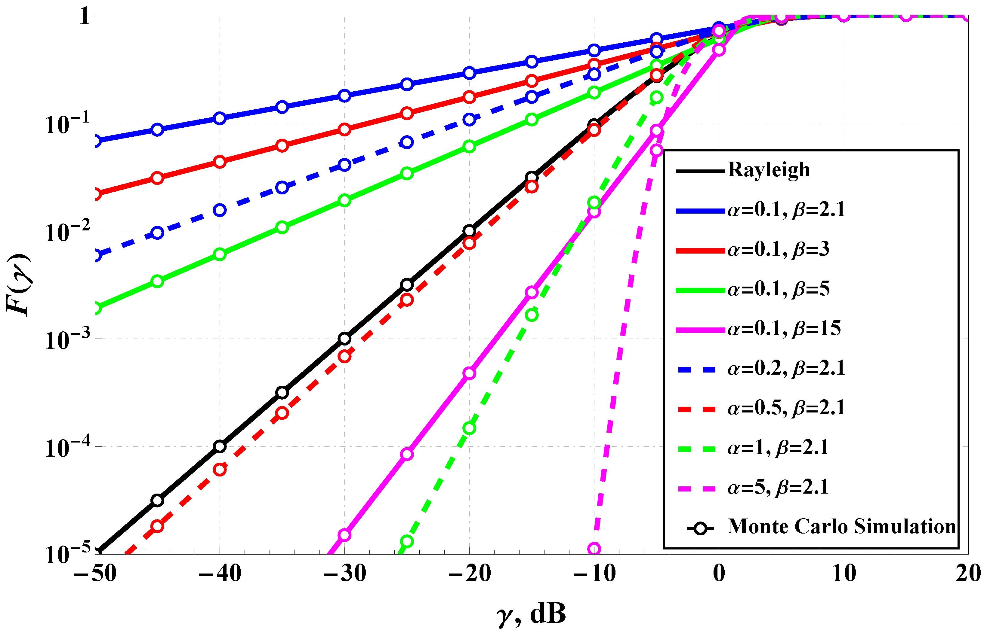
Figure 3.
IPL positioning among various fading channel models.
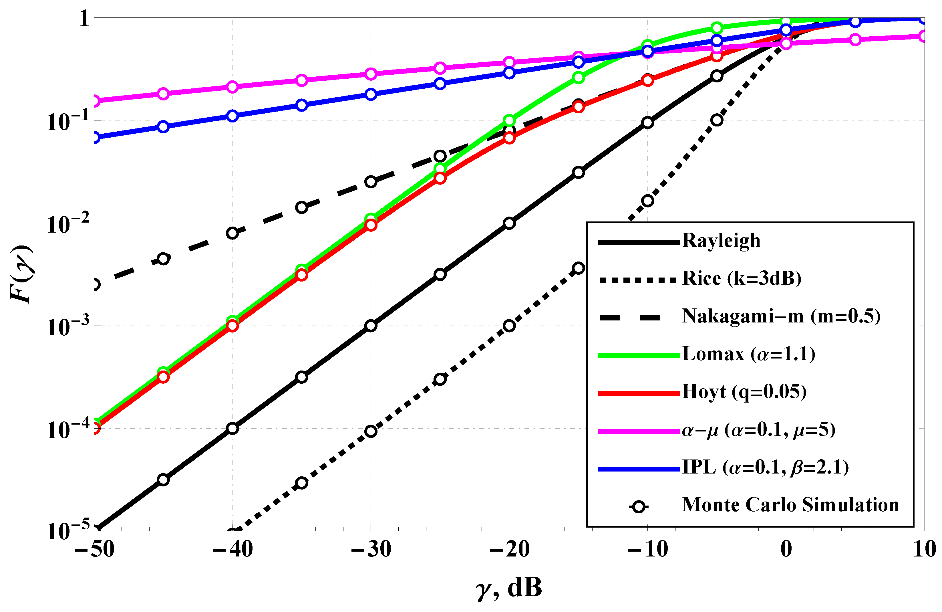
Figure 4.
MGF comparison of numerical evaluation and derived closed-form expression for various channel parameters.
Figure 4.
MGF comparison of numerical evaluation and derived closed-form expression for various channel parameters.

Figure 5.
Empirical data from D2D communication experiment with fitted IPL model and model: (a) LOS indoor environment (see [56] Figure 12a), (b) NLOS indoor environment (see [56] Figure 12b), (c) LOS outdoor environment (see [56] Figure 12c), and (d) NLOS outdoor environment (see [56] Figure 12d).

Figure 6.
Empirical data from D2D communication experiment [57] with fitted IPL model and model (see [42]).
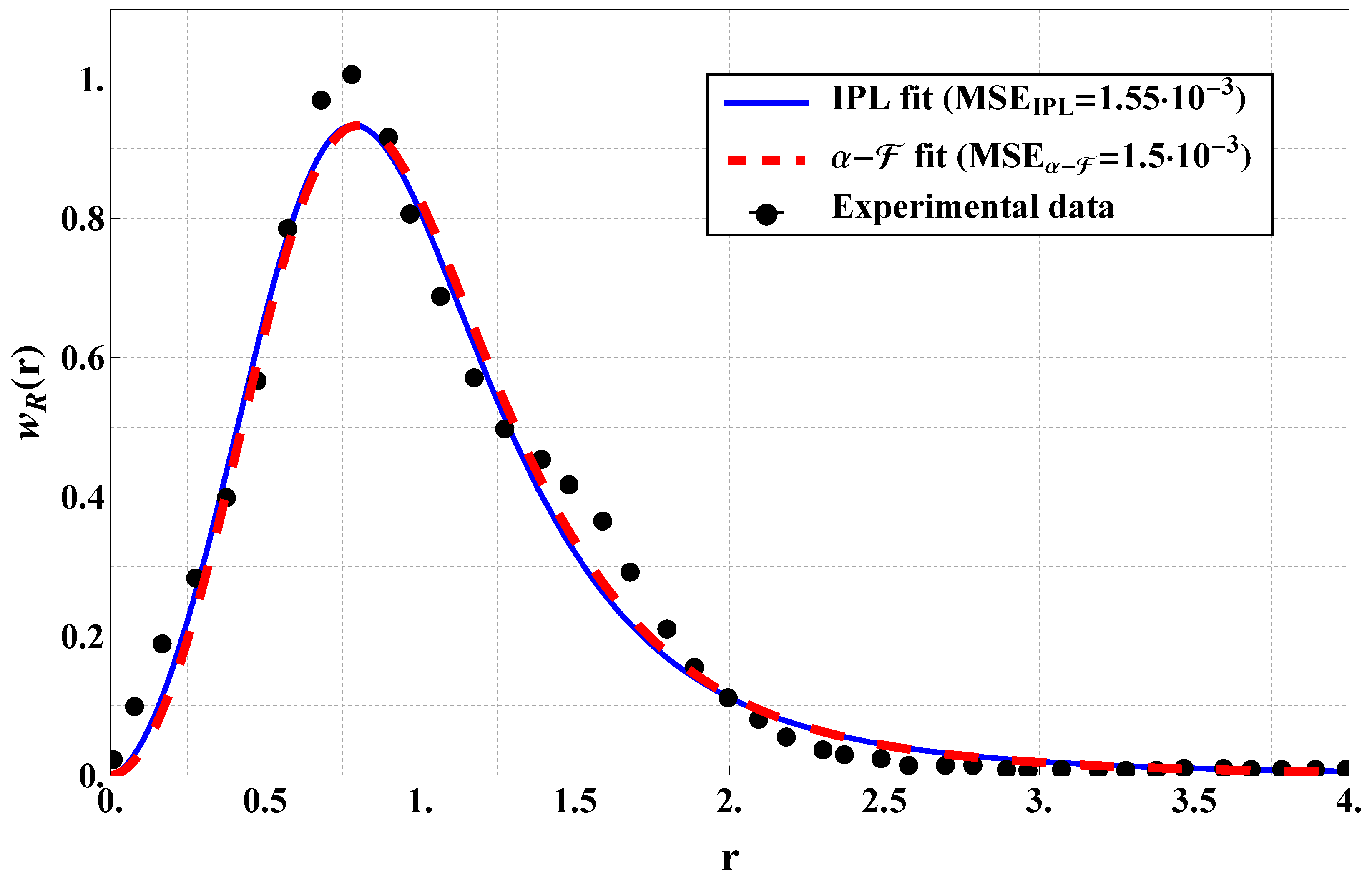


Figure 9.
AoF vs. channel parameters ().
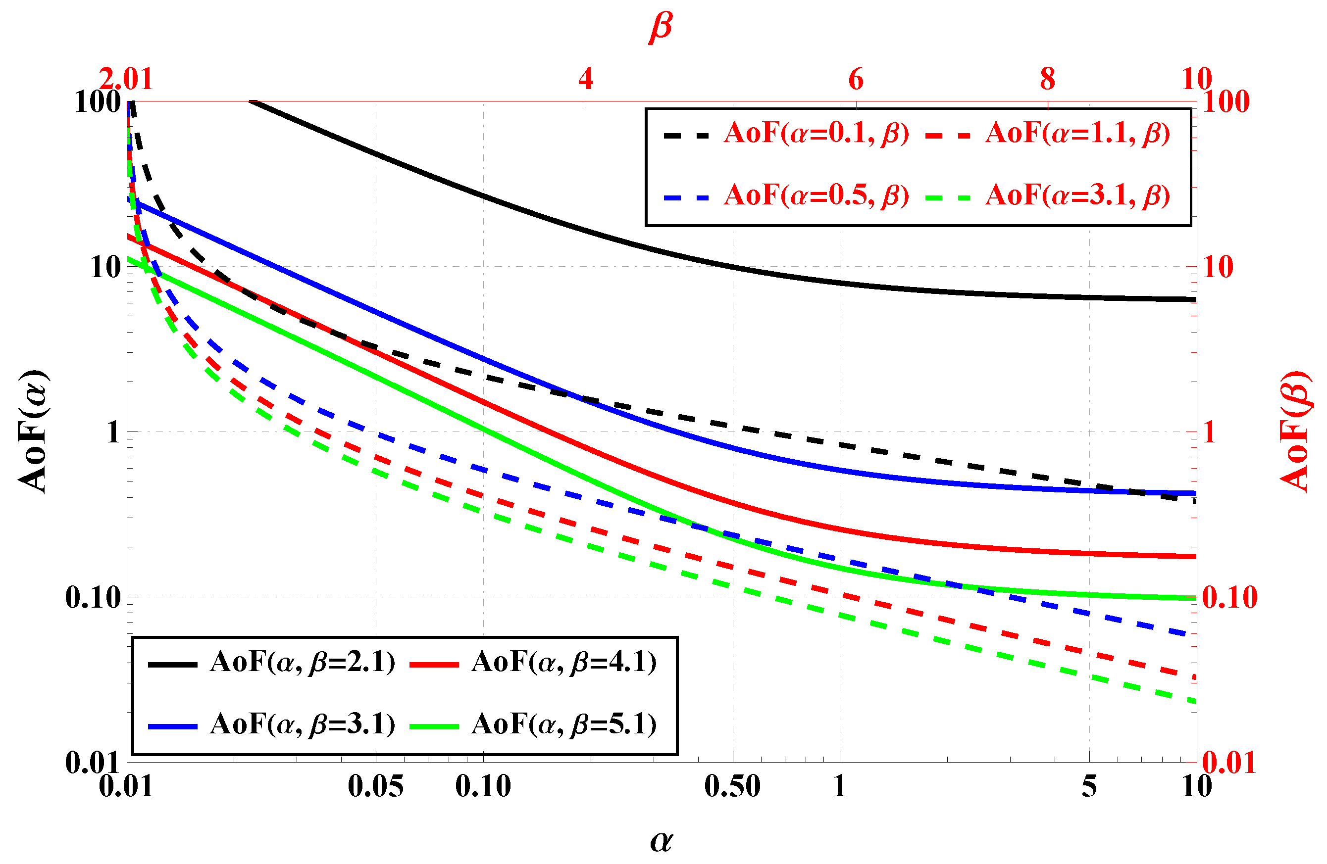
Figure 10.
Outage probability vs. for various channel parameters: (a) the impact for fixed small , (b) the impact for fixed small , and (c) the impact for fixed .
Figure 10.
Outage probability vs. for various channel parameters: (a) the impact for fixed small , (b) the impact for fixed small , and (c) the impact for fixed .
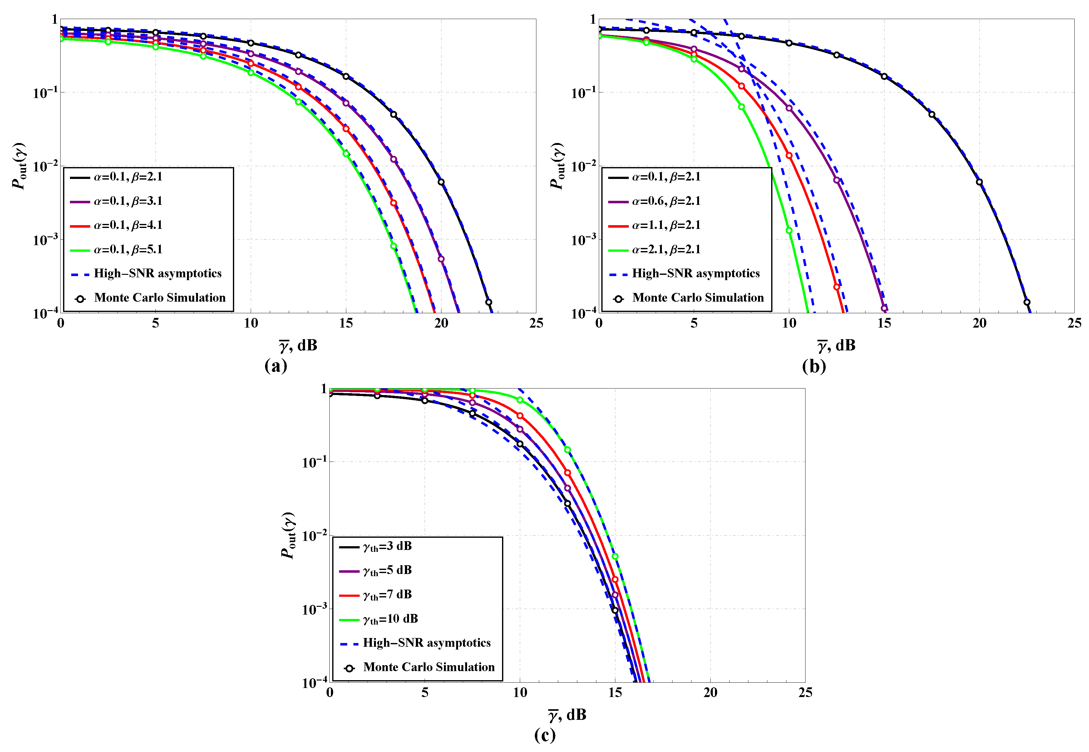
Figure 11.
ABER vs. for modulations and channel parameters: (a) the impact of constellation size for M-PSK with , (b) the impact of constellation size for M-QAM with , and (c) the impact of fading parameters for QAM-4.
Figure 11.
ABER vs. for modulations and channel parameters: (a) the impact of constellation size for M-PSK with , (b) the impact of constellation size for M-QAM with , and (c) the impact of fading parameters for QAM-4.
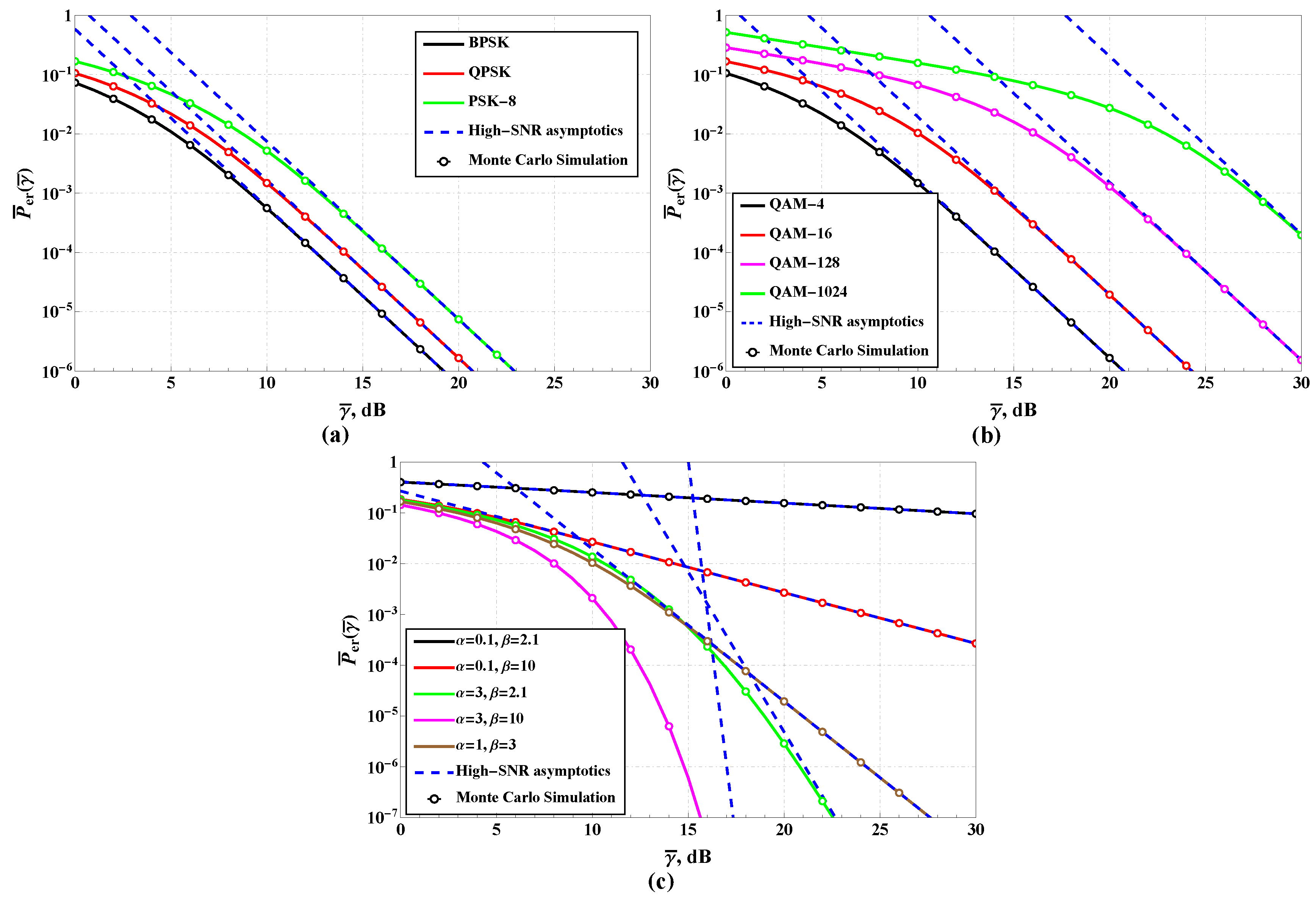
Figure 12.
IPL channel ergodic capacity vs. for various channel parameters ().

Figure 13.
Logarithmically scaled AoF contour map for various channel parameters (); black dashed line corresponds to Rayleigh fading.
Figure 13.
Logarithmically scaled AoF contour map for various channel parameters (); black dashed line corresponds to Rayleigh fading.
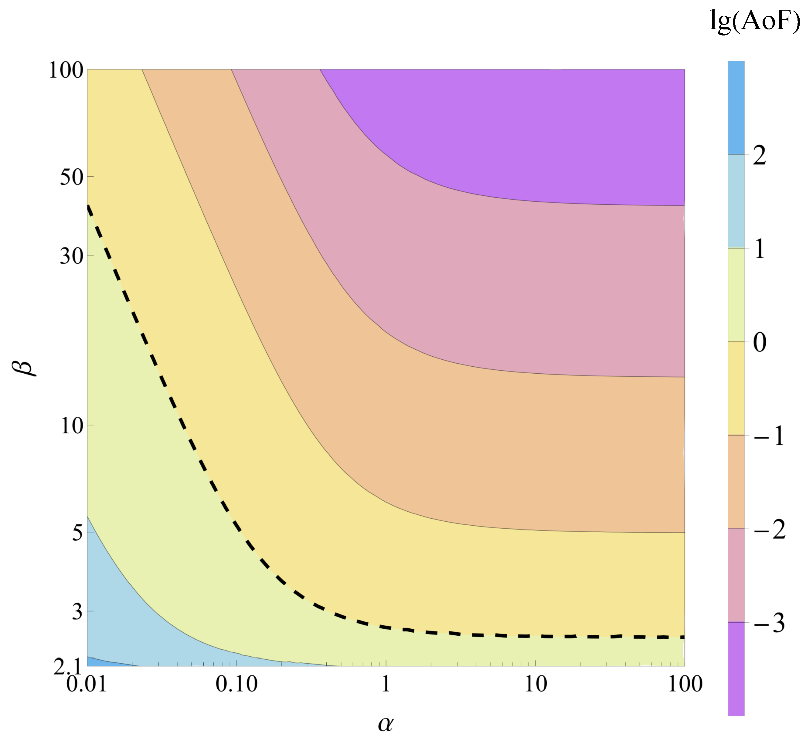
Figure 14.
contour map for various channel parameters (); black dashed line corresponds to , i.e., Rayleigh fading.
Figure 14.
contour map for various channel parameters (); black dashed line corresponds to , i.e., Rayleigh fading.


Table 1.
Modulation-specific coefficients for M-QAM and M-PSK.
| M-QAM | |||
| M-PSK |
Disclaimer/Publisher’s Note: The statements, opinions and data contained in all publications are solely those of the individual author(s) and contributor(s) and not of MDPI and/or the editor(s). MDPI and/or the editor(s) disclaim responsibility for any injury to people or property resulting from any ideas, methods, instructions or products referred to in the content. |
© 2024 by the author. Licensee MDPI, Basel, Switzerland. This article is an open access article distributed under the terms and conditions of the Creative Commons Attribution (CC BY) license (https://creativecommons.org/licenses/by/4.0/).
Share and Cite
MDPI and ACS Style
Gvozdarev, A.S. Closed-Form Performance Analysis of the Inverse Power Lomax Fading Channel Model. Mathematics 2024, 12, 3103. https://doi.org/10.3390/math12193103
AMA Style
Gvozdarev AS. Closed-Form Performance Analysis of the Inverse Power Lomax Fading Channel Model. Mathematics. 2024; 12(19):3103. https://doi.org/10.3390/math12193103
Chicago/Turabian StyleGvozdarev, Aleksey S. 2024. "Closed-Form Performance Analysis of the Inverse Power Lomax Fading Channel Model" Mathematics 12, no. 19: 3103. https://doi.org/10.3390/math12193103
Note that from the first issue of 2016, this journal uses article numbers instead of page numbers. See further details here.