Abstract
In an era of massive construction, damaged and aging infrastructure are becoming more common. Defects, such as cracking, spalling, etc., are main types of structural damage that widely occur. Hence, ensuring the safe operation of existing infrastructure through health monitoring has emerged as an important challenge facing engineers. In recent years, intelligent approaches, such as data-driven machines and deep learning crack detection have gradually dominated over traditional methods. Among them, the semantic segmentation using deep learning models is a process of the characterization of accurate locations and portraits of cracks using pixel-level classification. Most available studies rely on single-model knowledge to perform this task. However, it is well-known that the single model might suffer from low variance and low ability to generalize in case of data alteration. By leveraging the ensemble deep learning philosophy, a novel collaborative semantic segmentation of concrete cracks method called Co-CrackSegment is proposed. Firstly, five models, namely the U-net, SegNet, DeepCrack19, DeepLabV3-ResNet50, and DeepLabV3-ResNet101 are trained to serve as core models for the ensemble model Co-CrackSegment. To build the ensemble model Co-CrackSegment, a new iterative approach based on the best evaluation metrics, namely the Dice score, IoU, pixel accuracy, precision, and recall metrics is developed. Results show that the Co-CrackSegment exhibits a prominent performance compared with core models and weighted average ensemble by means of the considered best statistical metrics.
Keywords:
semantic segmentation; crack identification; ensemble learning; deep learning; Co-CrackSegment MSC:
68U10
1. Introduction
Structural health monitoring (SHM) and damage identification play a crucial role in ensuring the safe operation and structural integrity of in-service infrastructure [1,2]. SHM adheres to guarantee the continuous service of structures bearing internal and external loads and hazardous conditions [3,4]. These unwanted conditions can deteriorate structural elements and gradually lead to structural defects. Therefore, SHM serves as an essential maintenance framework for ensuring reliable infrastructure performance throughout their expected lifespan when subject to catastrophic events. Even if regular manual inspections deliver good information about structural conditions, they are often time-consuming, rely on human evaluations, and are susceptible to human errors [5,6]. In consequence, the utilization of intelligent, soft computing approaches has emerged as a more reliable and convenient method. Among them, convolutional neural networks (CNNs) are being implemented for data-driven defect identification. This can be achieved either through using 1D data as time-domain responses or using 2D data as originally captured images or time-frequence plots. For instance, image datasets gathered from a structure’s surface can be adapted to develop CNNs for image-based defect identification. A well-designed CNN can be an effective tool for crack identification, oiling the wheels of early damage detection and eliminating the risks of catastrophic events. This image-based CNN tool delivers smooth monitoring through taking advantage of machine intelligence to verifiably deduce features from training instances in a ductile manner more efficient than manual condition assessments [7,8].
The most common supervised image-based crack identifications using CNNs can be categorized into three main categories: (i) CNN-based classification methods directly try to recognize whether an image taken from a structure’s surface contains cracks by means of binary crack classification, or more complexly multiclass crack classification [9,10]. The total image is given a classification label, and the CNN learns to classify the images according to their labels. After training, the CNN classifier can be deployed for real-time crack identification without computationally expensive pixel-level tackling. Nevertheless, such category of methods fails to characterize and localize cracks in most scenarios without proper additional image processing techniques [11,12]; (ii) region-based methods are types of CNN-based tools that work on partial regions of the image and consider the cracks as objects that need to be detected. Methods such as sliding windows and You-Only-Look-Once (YOLO) [13] are common object detection tools that can be used to localize cracks by means of boundary boxes rather than tackling full-scale images or pixel-level features. These tools require the use of manually annotated ground truth bounding boxes that deliver supervision for the CNN or basic references for optimizing object possibilities. The output after training is given as the boundary boxes that identify the cracks from the backgrounds with confidence probabilities. Although the object detection tools are faster to train and deploy, they suffer from drawbacks such as the misidentification of crack boundaries and background voids [14,15,16]; (iii) semantic segmentation based on CNNs are modern pixel-level tools that adhere to precisely characterize cracks’ pixels and isolate them from the background pixels. Semantic segmentation uses two main procedures, namely downsampling and upsampling. The former reduces the spatial dimensions of feature maps and increases the number of filters/channels, while the latter increases the spatial dimensions of feature maps and reduces the number of filters/channels. In this case, the CNN assigns a probability of each pixel in the image according to its label, i.e., crack or non-crack, enabling it to generate binary-class attribute maps. The main advantages of semantic segmentation are the ability to characterize crack morphology and give more visual information about crack size and orientation. However, they require the manual preparation of ground truth images to train the CNN and can be computationally expensive in both training and testing. Given the advantages of the state-of-the-art sematic segmentation of concrete cracks, this paper aims to provide effective CNN-based semantic segmentation methods able to overcome the current challenges in this field [15,17,18,19].
Concrete crack detection usually holds several challenges related to crack shapes, widths, patterns, orientations, etc. Moreover, in case of image-based detection, other environmental factors contribute to make the automatic identification more difficult, such as shadows, lighting, foreign objects, rust, corrosion, etc. Image-based deep learning models can be trained to identify cracks of different widths from narrow cracks to wide cracks. Nevertheless, very narrow cracks might be more challenging, because the model might be too confused to see the difference between those cracks and other background textures [8]. Furthermore, crack structure images hold a contrast between the background and the crack itself, which affects the model detection efficiency. Background complex texture or varying background colors make the detection more difficult [14]. In addition, shadows and lighting conditions might reduce the resolution of crack area, which might degrade the model’s detection performance [15]. Hence, the pixel-level identification or the semantic segmentation can solve many of the aforementioned challenges, thanks to its ability to handle various crack widths and complex patterns. This is due to the pixel classification framework rather than treating the image as a whole. Moreover, the semantic segmentation models’ architectures are built in such a way that they perform downsampling and upsampling procedures guided by references of ground truth images. This helps to reduce the effect of environmental factors as well as eliminate light contrast challenges [12]. Therefore, the semantic segmentation can provide a reliable solution for crack-related detection challenges.
In recent years, CNN models such as Unet, SegNet, DeepLab, etc., have been successfully used for crack semantic segmentation. Although the single CNN model-based semantic segmentation has achieved major milestones in pixel-level crack identification, ensemble learning philosophy delivers renowned advantages via exploiting collective knowledge and diversity among ensemble core models. By training several CNN models either from the same type or different types and combining their predictions, they serve to improve the overall crack characterization and deliver more precise pixel crack/background probabilities. Therefore, ensemble learning can be more efficient than the single-model-based methods for concrete crack identification. Although traditional ensemble CNN models that involve the weighted average, bagging, stacking, and boosting have been used for image-based crack classification, they have been rarely applied in semantic segmentation of cracks. This is mainly because the pixel data are highly imbalanced and mostly belong to the background rather than the crack. Moreover, the pixel data are of high dimensions which make it difficult for meta learners to train and combine predictions and therefore require high computational efforts, especially in cases of stacking and boosting. Moreover, the averaging in weighted average and bagging methods might blur the pixels in crack boundaries, hiding their actual label probabilities. Therefore, it is of great importance to further adapt the ensemble learning philosophy for the purpose of crack semantic segmentation and propose more efficient methods similar to the current paper.
2. Literature Review, Research Gaps, and Contributions
Several research works investigated the application of CNNs for concrete crack semantic segmentation with a main focus on single model-based approaches. For example, Arafin et al. [20] developed a multistage strategy for classification and the semantic segmentation of concrete defects with promising results. First, the classification of cracks and spalling defects was performed using three CNNs, namely the InceptionV3, ResNet50, and VGG19, with reported 91% accuracy for InceptionV3. Also, the semantic segmentation was employed based on the Unet and PSPnet to identify defects’ areas with an average evaluation metrics score over 90%. In another work, Hang et al. [21] developed the AFFNet that used the ResNet101 as backbone and dual attention mechanisms for the semantic segmentation of concrete cracks with higher mean intersection over union (IoU) metrics over 84%. Tabernik et al. [22] developed the SegDecNet++ for the semantic segmentation of concrete and pavements cracks and enhanced classification-based segmentation reporting a Dice score of 81%. Shang et al. [23] proposed a fusion-based Unet for the pixel-level identification of sealed cracks with an IoU over 84%. In other research [24], the multiresolution feature extraction network (MSMR) was developed for the semantic segmentation of concrete cracks with a reported IoU over 82%. Minh Dang et al. [25] developed a semantic segmentation of sewer defects method via utilizing the DeepLabV3+ with various backbone networks and reported an accuracy of 97% and IoU of 68%. Another semantic segmentation model was developed by Joshi et al. [26], in which three submodules were incorporated and transfer learning was utilized to improve the overall segmentation results. In addition, a multistage YOLO-based object detection and Otsu thresholding for crack quantification purpose was proposed by Mishra et al. [27]. Further research was conducted by Shi et al. [28], in which they proposed what was called the multilevel contrastive learning CNN for crack segmentation. The developed approach incorporated a dual training approach using full image and image patches with prespecified sizes, and the contrastive learning was then used to provide the final decision about the pixel labels. The overall reported IoU for different scenarios did not exceed 70% for all tested datasets. More research was conducted by Savino and Tondolo [29], in which the Deeplabv3+ networks were developed with weights initialization using transfer learning of different other networks, with the highest reported accuracy bring over 91%. Hadinata et al. [30] developed a multiclass segmentation approach for three classes of cracks, spalling, and voids using the Unet and DeepLabV3+, with a mean reported IoU of around 60% using the Unet. Another approach for crack semantic segmentation using a hybrid deep learning approach based on class activation maps and an encoder–decoder network was proposed by Al-Huda et al. [31]. By incorporating image processing methods and transfer learning, the proposed approach was able to provide a mean IoU of around 90%. In addition, Ali et al. [32] utilized the local pixel-weighing approach with residual blocks for improving a CNN with an encoder–decoder section, with average accuracies over 98% for different scenarios. Kang et al. [33] utilized the faster RCNN to allocate crack boundaries and a modified tubularity flow field for segmentation; a mean average IoU of 83% was reported. Also, the crack semantic segmentation of nuclear containments was conducted with an improved Unet using multifeature fusion and focal loss. Compared with other approaches, the proposed approach achieved a better IoU value of over 73%. From the studied literature, it can be seen that the development and deployment of a single model and its improved features or hybrid versions for the task of crack semantic segmentation is the common research trend worldwide. However, single models are often susceptible to low generalization abilities and might not recognize all underlying crack patterns. In addition, the high bias of the considered datasets might contribute to decline in the performance of single-model-based approaches.
In machine learning applications, ensemble predictions often contribute to improve the individual model predictions, especially when performance of individual models drops with data alterations [34,35,36]. In recent years, several attempts were devoted to implement ensemble learning for semantic segmentation applications [37,38,39]. Difficulties with the high computational cost to train individual models to deal with pixel-level data make ensemble learning less favorable in the case of semantic segmentation. Besides the semantic segmentation of cracks, several successful attempts were reported in the literature. For example, Bousselham et al. [40] developed an ensemble model based on a single meta-learner via leveraging a multifeature pyramid network for semantic segmentation, which was tested using general benchmarking datasets. Nigam et al. [41] developed an ensemble deep learning semantic segmentation model via extracting knowledge, using training individual models on separate data sources and fine-tuning after transfer learning to the intended domain with the main dataset which drone-collected scenes of image data. Also, three DeeplabV3 models trained using the firefly algorithms were ensembled by Zhang et al. [42] by applying model averaging for the semantic segmentation of several benchmark datasets. In other research, Lee et al. [43] developed an ensemble learning model via the progressive weighting of several core models and their backbones for segmentation of skin lesions. Three Unet models with different backbones were ensembled using the model averaging and further tuned with an evolutionary algorithm for retinal vessel segmentation. For crack semantic segmentation purposes, few research works have been concerned with the use of ensemble learning. However, some few papers applied the ensemble learning for crack semantic segmentation, such as the work of Lee et al. [44], who developed a meta-model architecture to synthesize an ensemble prediction of four models, namely the DeeplabV3, Unet, DeepLabV3+, and DANet, with better results reported for the case of the meta-learner ensemble. Li and Zhao [45] attempted to ensemble six models, namely the PSPNet, Unet, DeepLabv3+, Segnet, PSPNet, and FCN-8s by using four softmax regression-based models. Amieghemen and Sherif [46] employed the weighted ensemble of four models, namely three Unets with different backbones and the PaveNet, for the semantic segmentation of aerial images including pavement cracks. In another work, the fuzzy integral was used to ensemble three Linknet models with three different backbone architectures for the purpose of pavement crack segmentation [47]. Similar other research works can be found in [48,49,50,51,52,53]. A recent review article has indicated that the use of ensemble learning for the semantic segmentation of concrete cracks is less popular to minimize the overfitting and low variance of deep neural networks models [54]. From the above literature, it is evident that research on crack semantic segmentation using ensemble learning is still premature and needs further improvements.
According to the aforementioned literature survey, the major research gaps can be listed as the following:
- Most available studies relied on individual model prediction to perform the crack semantic segmentation. Nevertheless, it is well-known that the individual model might suffer from low variance and low generalization ability in case of data alteration.
- To overcome the overfitting of crack image data, many studies focus on various hybridizations or modifications of existing models as well as transfer learning, which still do not incorporate the knowledge of multiple learning to perform the concrete semantic segmentation task.
- Crack semantic segmentation underlies several problems, particularly when dealing with complex and highly contaminated image backgrounds, blurring, shadows, etc. Therefore, it is necessary to improve the existing identification method and include novel techniques.
- The ensemble learning is a very effective method to improve the performance of individual learners through combining their knowledge using some well-established methods, such as weighted averaging, stacking, bagging, and boosting.
- For pixel-level semantic segmentation, especially in case of crack images, the abovementioned ensemble learning methods are less popular among researchers. This is mainly due to problems related to computational cost and difficulties in optimizing ensemble learning parameters.
- The traditional weighted average ensemble learning for pixel-level semantic segmentation might suffer from pixel blurring of the crack boundaries, resulting high bias of predicted crack map than the ground truth.
- It is well-known that pixel-level semantic segmentation is of high spatial correlation features which do not highly suit the independent sampling of supervised learning. Moreover, as most pixels belong to background and to crack area, class imbalance is inevitable in pixel-level crack detection. These two reasons make the use of traditional ensemble learning such as boosting and stacking difficult.
- Hence, it is of great significance to improve the existing ensemble learning methods for pixel-level semantic segmentation, especially when considering crack images that naturally include various background contaminations.
To tackle the abovementioned research gaps, this article introduces a new ensemble learning model for solving the problem of pixel-level semantic segmentation of concrete cracks. The main contributions of the current research can be summarized as follows:
- By leveraging the ensemble deep learning philosophy, a novel collaborative semantic segmentation of concrete cracks method called Co-CrackSegment is proposed.
- Five models, namely the U-net, SegNet, DeepCrack19, and DeepLabV3 with ResNet50, and ResNet101 backbones are trained to serve as core models for the Co-CrackSegment.
- To build the collaborative model, a new iterative approach based on the best evaluation metrics, namely the Dice score, IoU, pixel accuracy, precision, and recall metrics is developed.
- Finally, detailed numerical and visual comparisons between the Co-CrackSegment and the core models as well as the weighted average ensemble learning model are presented.
The remainder of the paper is outlined as follows: (i) the proposed method of the semantic segmentation of surface cracks is presented in Section 3; (ii) the results and discussion of implementation of the proposed Co-CrackSegment with overall evaluation and comparison are illustrated in Section 4; (iii) and finally, the conclusions of this work are presented in Section 5.
3. Materials and Methods
In this section, a full description on the mathematical background of the semantic segmentation problem, adopted datasets for semantic segmentation, as well as the core deep learning models used in the Co-CrackSegment model are presented. Moreover, an overview of the proposed Co-CrackSegment model including the iterative optimal evaluation metric-based ensemble approach is given in detail.
3.1. Mathematical Background on Deep Learning-Based Semantic Segmentation
Semantic segmentation is a fundamental task in computer vision that aims to appoint labels to image pixels. In other words, semantic segmentation is considered a pixel-level classification problem that aims to classify each pixel in an image rather than a total object. When considering the semantic segmentation of concrete cracks, each pixel can be given one of two labels, namely crack or non-crack labels. This helps to accurately and precisely localize and identify a defect area within the concrete surface [55]. In this regard, the problem of the semantic segmentation of an image, , can be interpreted as a pixel-wise classification problem, where the target is to allocate a label, , to each concrete surface pixel. To solve this problem, the deep CNNs with special encoder–decoder architectures similar to the U-net, SegNet, DeepLab, etc., are utilized.
To further provide a mathematical interpretation of the semantic segmentation problem, consider the input-colored image having channels with width and height (), and the label , where are the pixel indices and is the number of classes ( for the pixel-level semantic segmentation of concrete images). The main aim is to define a mapping function that provides a probability distribution of labels around the image pixels [56], which can be mathematically expressed as
where is the predicted label for pixel and the CNN with a special encoder–decoder architecture is trained and optimized through minimizing the error between the ground truth labels and the predicted labels . This implies the use of loss functions such as the Dice loss function, which is derived using the Dice coefficient, that measures the overlap between the predicted labels of image pixels and the ground truth and can be given for a single class as [57,58].
where and are the number of pixels of the predicted and ground truth labels, respectively, and is the intersection between the predicted and ground truth labels. It is worth mentioning that the Dice value of one indicates a full overlap, and vice versa.
However, in order to use the Dice coefficient as a loss function, it is necessary to calculate the complement of the Dice coefficient and minimize it, or in other words maximize the overlap, which can be written for binary semantic segmentation as in Equation (3). Furthermore, an expanded Dice loss expression for pixel-level values can be provided in Equation (4) [57,58].
where is the total number of image pixels, and and are the predicted and ground truth pixel probabilities.
Hence, the pixel-level classification or the semantic segmentation problem can be formulated as finding function , which corresponds to the minimum total loss by using Equation (5).
For the semantic segmentation of concrete cracks, the deep learning models are trained via calculating the gradients of the loss function (Dice loss in this case) with respect to CNN parameters, namely weights and biases by applying the backpropagation. The calculation of gradients helps to formulate the optimization problem through various sorts of optimization algorithms such as Adam or gradient decent approaches. Thereafter, the model parameters are updated iteratively aiming to reduce the Dice loss so that pixel-wise classification accuracy increases via achieving maximum overlap between the ground truth and the predicted pixel probabilities. This iterative process is executed using several epochs along the dataset and the semantic segmentation accuracy is improved for the best pixel-level semantic segmentation of concrete cracks.
As it has been mentioned above, in order to tackle the semantic segmentation problem of concrete cracks, the deep CNNs with the special encoder–decoder designs are utilized. The encoder function is to extract features form input images (downsampling) using a series of convolution and pooling operations followed by an activation function. As the spatial information of the feature maps cringe, the CNN learns complex features that capture pixel-level information of the cracks in the image [58]. Mathematically, the output feature map of the encoder at layer for output channel k can be calculated as
where is the output feature map at pixel at layer L for output channel K, while to denote the input feature map from the previous layer L − 1 for a specific input channel c, we can write . and are the convolutional filter or weight matrix and biases at the layer , respectively, and and are the dimensions of the convolution mask, and is the activation function.
The max-pooling operation is often applied afterwards to reduce the spatial resolution of the feature maps in which can be given as [59].
where is the scale of spatial dimensions reduction.
In the decoder section, the feature maps are upsampled to recover spatial information and map the features back to the input space. In general, the decoder underlies a series of upsampling operations, where every type of semantic segmentation model might apply different types of upsampling based on its design. Common operations involve the transposed convolution, skip connections, etc. The typical transposed convolution for each pixel in the feature map at layer can be expressed as
where is the up-ampled feature map at location , is the feature map from the previous decoder layer L − 1 for input channel c, and and are the convolutional filter or weight matrix and biases at the layer , respectively.
In CNNs like U-Net and DeepLab, skip connections are utilized to merge the encoded low-level feature maps with the upsampled features in the decoder to hold over the spatial features. The element-wise addition of encoder and decoder feature maps can be expressed as Equation (9) describes [60]
where is the skip connection feature map, is the feature map from the encoder at layer , and is the element-wise addition.
After the skip connection, a set of convolution operations should be applied to the results of Equation (11) as follows
where is the feature map resulted after skip connections, and are the convolutional filters applied to the upsampled feature map .
The final layer of the decoder applies the softmax or sigmoid activation functions to the upsampled feature map to generate a pixel-wise classification, where the softmax is used in case of multiclass semantic segmentation (as in Equation (13)) and sigmoid (as in Equation (14)) is used in the binary case that is the case of pixel-level semantic segmentation of concrete cracks. This operation can be expressed as [61,62]
where is the logit for class , is the probability of having the class , and is the number of classes.
Finally, by combining the aforementioned decoder equations, the generalized decoder equation can be written as
where () is the transposed convolution, and is the convolution operation.
3.2. Crack Semantic Segmentation Framework
The overall common crack semantic segmentation comprises six key stages that can be summarized as follows: (i) image data gathering; (ii) image preprocessing and ground truth image dataset construction; (iii) semantic segmentation model architecture and training algorithm determination; (vi) semantic segmentation model training and testing; (v) crack map identification; and (vi) results reporting. The raw crack image dataset is preliminary collected from a considered structure such as flying drones, camera holders, climbing robots, etc. After that, the dataset should undergo some data preprocessing procedures, in which the dataset undergoes image cropping, scaling, augmentation, labeling, normalization, etc. Thereafter, the ground truth images of the dataset are built, which provide the main comparison tools inside the semantic segmentation models. Then, the dual dataset of preprocessed images and their ground truths are divided into training and testing subsets. Subsequently, the semantic segmentation model design and parameters as well as the training method are determined. Then, the semantic segmentation model is trained until approaching a good accuracy. After training the model, the model is evaluated and the crack maps are determined. Finally, the final spatial locations of the cracks are reported. The overall semantic segmentation is realized in Figure 1.
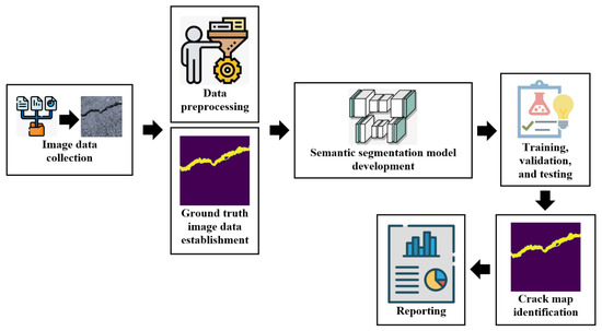
Figure 1.
The general crack semantic segmentation framework.
3.3. Datasets
In this research, two public datasets were adopted. The first one was the famous DeepCrack dataset which was developed by Liu et al. [63]. The DeepCrack dataset was composed of 537 concrete and Asphalt images with their manually annotated ground truth images. This dataset was divided into 85% for training and 15% for testing. The dataset included many challenging aspects such as cracks with shadows, cracks with foreign objects, spalling, complex background, cracks with rust and marks, etc. Some representative images and their ground truth masks are presented in Figure 2.

Figure 2.
Sample images of the DeepCrack dataset [63].
Another larger and well-known dataset for crack segmentation is the Rissbilder dataset [64,65], which contains 3249 training and 573 testing images divided into 85% for training and 15% for testing. The dataset includes wall images taken by a climbing robot. The data are very challenging, containing shadows, illumination, foreign objects, crack-like scaling, crack-like background texture, thin cracks with dirty background, etc. The utilization of this dataset helped to provide complex instances to the developed semantic segmentation methods and verify their performances. Some image samples and their ground truth masks are presented in Figure 3.
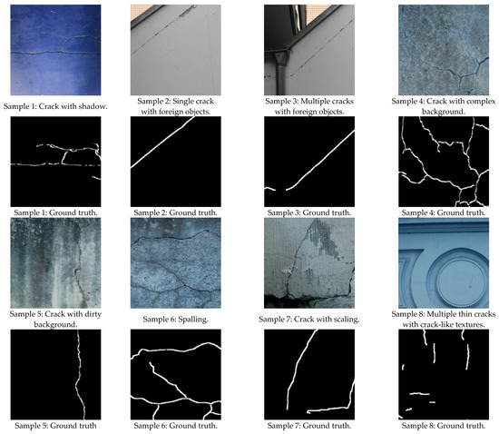
Figure 3.
Sample images of the Rissbilder dataset [64,65].
As the proposed method was an ensemble learning method, the cross validation in this case was less preferable, because when testing the ensemble learning semantic segmentation models with the core models, it was important to maintain a custom testing data to deliver an unbiased and reliable comparison. In addition, for practical deployment, the semantic segmentation models were used to provide a decision on the new data; therefore, the use of fixed test data was more practical than the cross validation. Moreover, semantic segmentation models require high computational efforts, because images are of two-dimensional shape and are of high resolution. Moreover, the ensemble learning requires more computational time, making the use of cross-validation increases the computational burden. Furthermore, semantic segmentation deals with spatial locations of pixels; therefore, using a fixed partitioning of data was more preferable, because the random portioning of patches or pixels when applying cross validation could violate the relationships between the input images and ground truth feature maps.
3.4. The Core Models
3.4.1. The U-Net
One of the most famous semantic segmentation deep CNNs is the U-net, which was originally proposed by Ronneberger [66] for medical imaging segmentation applications. However, the U-net has been utilized in various semantic segmentation projects afterwards. The U-net was named due to it architecture that takes the portrait of the U-frame of encoder–decoder paths. The encoder path grasps the semantic features of the image via applying the basic CNN module, in which the image is subject to downsampling through employing Conv. and pooling operations. Nevertheless, the encoder part endeavors to precisely recuperate spatial features through applying a set of upsampling and Conv. operations. The high-order feature maps from the encoder are merged with the upsampled feature maps using skip connections, which permits for the efficient recovery of low-level spatial features. The main merit of the U-net is the capability to recuperate and merge local and global features using the encoder–decoder pair and skip connections that help to deliver accurate pixel-level classification even with small datasets. The accurate identification of crack boundaries makes it very effective for semantic segmentation applications, especially in the case of crack semantic segmentation. The architecture of U-net can be observed in Figure 4.
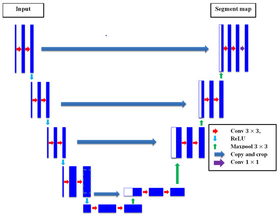
Figure 4.
The U-net architecture.
3.4.2. The SegNet
Another well-known network architecture that was used for semantic segmentation tasks was the SegNet, which is a type of CNN with an encoder–decoder pair model originally proposed for road scene segmentation. The main tool of the SegNet was the transfer learning of the VGG-16 architecture into the decoder module to recuperate pixel-level special and semantic features employing the Conv. and pooling operations of the VGG-16. The innovative point of the SegNet was the design of its decoder, in which the unpooling operation was proposed to unsample low-level features coming from the encoder. The indices of the maxpooled features taken from the encoder were utilized to upsample the higher features helping to maintain boundaries and spatial features, which made it very suitable for crack semantic segmentation applications. The main implemented operations in the SegNet were the full convolutions instead of fully connected layers which enable it to process inputs of various dimensions, the skip connections that contributed to combine the high-level features from the encoder with the upsampled features of the decoder which boosted semantic segmentation accuracy, and the use of transfer learning VGG-16 helped to keep the minimum number of training parameters and contributed to lower computational efforts. The overall merits of SegNet made it an excellent choice for the semantic segmentation of cracks, hence it was adopted in this work as a main core model. The design of SegNet can be realized in Figure 5.
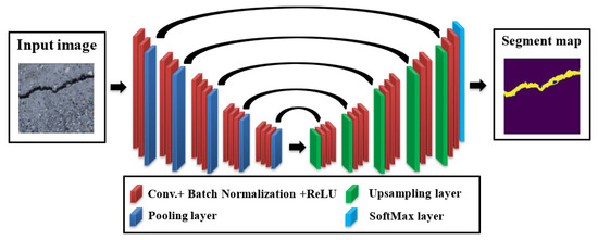
Figure 5.
The SegNet architecture.
3.4.3. DeepCrack19
A well-established CNN model which was designed particularly for concrete crack identification and segmentation is the DeepCrack19 [63]. This model leverages the popular encoder–decoder pair structure with skip connections similar to other semantic segmentation models. The encoder part that does the downsampling is made of a VGG-19 [67] model previously trained using the ImageNet dataset. It is composed of 19 Conv. layers with 5 maxpool layers. The decoder branch uses the same idea of upsampling and skip connections to merge the encoder-resulted upsampled low-level feature maps and the unsampled high-level feature maps to provide a concise semantic segmentation of cracks. The training process of this network elaborates a double loss function, namely the cross entropy and the Dice loss to optimize pixel-level classification of minor cracks. It is well-known that predictions from lower order Conv. layers efficiently maintain crack boundaries but are susceptible to noise, and while deeper layers are robust against noise, they might not be able to keep concrete boundaries. DeepCrack19 proposed a compromise solution to solve this problem through introducing the guided filtering operation in which the model generated a binary crack mask from a fused prediction of various Conv. layers and then utilized the output of Conv.1 and 2 layers as a guiding tool. Thereafter, the guided filtering was implemented to deliver the final classification. The overall DeepCrack19 model can be well-understood in Figure 6.
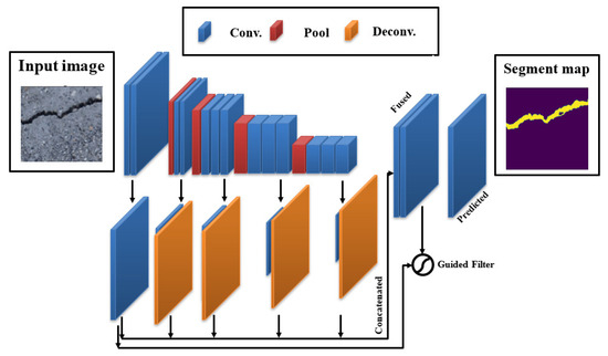
Figure 6.
The DeepCrack19 architecture.
3.4.4. The DeepLabV3 with Backbones
Based on DeepLab model and developed by Google, DeepLabV3 is a relatively new deep learning model for semantic segmentation [68]. The DeepLabV3 employed several new techniques to improve prediction. The main novelty of this model was the replacement of the convolution operation with the dilated or atrous convolution to recuperate the multiscale features without adding extra computational efforts. The atrous convolution implemented dilation rates between the filter values, which efficiently increased the filter field of observation without altering its size. In addition, the DeepLabV3 used what is called the atrous spatial pyramid pooling to perform a multiscale object segmentation which used a parallel approach incorporating atrous operations with various dilation rates. In addition, the DeepLabV3 utilized a simple type of decoder module to purify the semantic segmentation outcomes, which can be very useful in the case of segmenting crack boundaries. Furthermore, the bilinear sampling and concentration was conducted using the decoder which merged both low- and high-level feature maps, which in turn helped to recover the accurate spatial information of crack boundaries. The DeepLabV3 had the feature of coupling various backbone architectures similar to U-net. In this work, two ResNet models, which are the ResNet50 and ResNet101, were merged within the DeepLabV3 for the purpose of the semantic segmentation of structural cracks. The use of ResNet50 backbone held an advantage of powerful residual and skip connections to overcome the gradient vanishing problem during the training process. In addition, the use of ResNet101 as a backbone helped to improve the accuracy because the ResNet101 is double in depth of ResNet50 and can be useful in performing better extractions of the complex crack pixel features. However, the use of DeepLabV3/ResNet101 was more computationally expensive in comparison, especially when using large datasets. The architecture of DeepLabV3 with backbones can be seen in Figure 7.
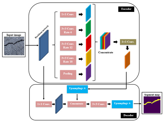
Figure 7.
The DeepLabV3 with backbones architecture.
3.5. Training Procedure
To train the core models, the input crack images were resized to pixeled RBG images and the pixel values normalized between 0 and 1. Data augmentation was applied to improve the variability of the images using random rotation, horizontal and vertical flipping, normalization, and random color jittering. The core models were evolved by considering a batch size of 8 and with 40 epochs. The Dice loss function was implemented to measure the difference between the predicted and ground truth masks. Other related parameters can be observed in Table 1 with respect to dataset1 and dataset2, respectively.

Table 1.
The training parameters of datasets 1 and 2.
The data augmentation was only applied to the training data for both datasets. Applying data augmentation to the total training image data helped to boost the efficiency and performance of the core and ensemble semantic segmentation models. Data augmentation contributed to increase the diversity and complexity of crack instances through adding more environmental effects, different crack angles, a wider range of scenarios, etc. This highly helped to boost the semantic segmentation models’ performances and increase the generalization to see beyond the original training data. Furthermore, concrete crack datasets often include rare cracking cases and imbalanced crack pixels class compared to background pixels class. Therefore, data augmentation could partially solve the imbalanced data problem via adding more instances to the training data. In addition, data augmentation introduced some controlled variations or noise to the training data, contributing to achieve better regularized semantic segmentation models and improve their abilities to tackle real-world data. Here, it is worth mentioning that the data augmentation should not be applied to testing data, because it can violate the basic rule of “Independent and Identically Distributed” data. In other words, the training and testing data should be independent and taken from the same probability distribution. This is due to the fact that data augmentation applies transformations that might lead to similarities and correlations between the original and augmented data. Furthermore, it can degrade the performance evaluation, because the model will deal with real-world images after deployment.
3.6. Evaluation Metrics
The main sets of evaluation metrics for semantic segmentation were categorized under overlapping metrics, in which the semantic segmentation model measured the overlap of pixels between the original image segmentation map and ground truth. To compute the semantic segmentation evaluation metrics, the confusion matrix of pixel-based segmentation mask was the starting point. The confusion matrix was composed of true (TP) and false positives (FP) as well as false (FN) and true negatives (FN). The main overlap metrics were the Dice and intersection over union (IoU) metrics, in which a one-prediction corresponded a full overlapping, whereas a zero-prediction was associated with an absence of overlapping between the predicted mask and ground truth. The Dice score and IoU can be calculated as follows:
and
Or in terms of confusion matrix, the Dice score and IoU can be calculated as follows:
and
Furthermore, the Rand score (pixel accuracy) is the number of correct pixel predictions (TP and TN) divided by the total number of pixel predictions, as in the following equation:
In addition, the precision and recall are popular evaluation metrics in semantic segmentation. Precision measures how often predictions for the positive class are correct in the segmentation result, while recall represents how well the semantic segmentation model detects all positive pixels in the segmentation result. The precision and recall can be calculated as follows:
and
Finally, the mAP, which is the mean average precision or the average value of precision across all classes, is utilized. The mAp can be given as
where k is the number of classes in the segmentation problem.
3.7. The Proposed Group Learning Method
Crack semantic segmentation is often a challenging task, particularly when dealing with complex and contaminated image backgrounds. The available identification approaches require improvements, and advanced techniques must be employed. Group learning or ensemble learning are common tools that improve single classifiers via combining their predictions. However, these group learning tools are less common to be applied for pixel-level semantic segmentation [63], especially for crack images due to computational costs and difficulties in optimizing ensemble learning parameters for pixel-level evaluation. Therefore, it is of high significance to boost existing ensemble learning methods for pixel-level semantic segmentation for crack images. To address this issue, a novel cooperative crack semantic segmentation method, called Co-CrackSegment is proposed. This method takes advantage of ensemble deep learning philosophy through developing a new iterative approach based on the optimal evaluation metrics. Five Co-CrackSegment frameworks using the optimal Dice score (Co-CrackSegment/Dice), optimal IoU (Co-CrackSegment/IoU), optimal pixel accuracy (Co-CrackSegment/Pixel_Acc), optimal precision (Co-CrackSegment/Precision), and optimal recall (Co-CrackSegment/Recall) were developed and compared. To construct the group learner, five models, namely the U-net, SegNet, DeepCrack19, and DeepLabV3 with ResNet50, and ResNet101 backbones were trained to serve as core models for the Co-CrackSegment. The N trained core models were inserted in a model list and an external archive that stores the best model metrics. Each testing image was fed to the trained models and the evaluation metrics were computed subsequently including the current evaluation metrics. Thereafter, the external archive was altered and the model evaluation metrics were stored if a better evaluation metric score was achieved for each of the Co-CrackSegment frameworks. Finally, the overall iterative method was terminated after the best trained models’ metrics were stored. The overall approach can be realized in Figure 8 as well as the following pseudo code:
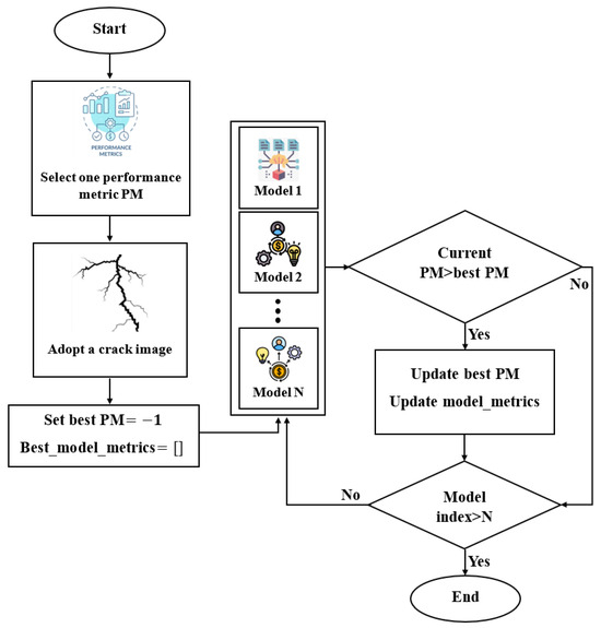
Figure 8.
The developed collaborative Co-CrackSegment semantic segmentation approach.
- Load N trained semantic segmentation models in the model_list.
- Choose one Co-CrackSegment framework, namely Co-CrackSegment/Dice, Co-CrackSegment/IoU, Co-CrackSegment/Pixel_Acc, Co-CrackSegment/Precision, or Co-CrackSegment/Recall.
- Set best_evaluation_metric_score to −1, and best_model_metrics to an empty matrix.
- For each test image, conduct the following:
- (a)
- For each current_model in the model_list (N times)
- (b)
- Set the trainer.model to the current_model.
- (c)
- Evaluate current_model with test image and compute the segmentation prediction output.
- (d)
- Compute the overall evaluation metric scores including the current_evaluation_metric_score of the test image (current_model_metrics).
- (e)
- If (current_evaluation_metric_score >best_evaluation_metric_score)
- i.
- best_evaluation_metric_score = current_evaluation_metric_score
- ii.
- best_model_metrics= current_model_metrics
- iii.
- Add trainer.model to the evaluation results matrix.
- Show the results.
To better understand the proposed Co-CrackSegment method, the pseudo code and Figure 8 are further explained. The Co-CrackSegment started with loading a group of pre-trained semantic segmentation models into a list called model_list (5 models in this case). Then, a performance metric (PM) was chosen for model evaluation and ensemble, namely the precision, recall, pixel accuracy, Dice score, or IoU. This PM was used to check the performance of each model in the model_list. The Co-CrackSegment then initialized two main variables, namely the best_evaluation_metric_score which was set to −1, and the best_model_metrics which was set to an empty archive. The best_evaluation_metric_score aimed to store the highest PM score achieved so far and the best_model_metrics was used to save the best model’s overall performance metrics. For each crack image, an iterative procedure was conducted via testing each model of the model_list. For each semantic segmentation model, the Co-CrackSegment algorithm set the trainer.model to the current model, which was evaluated on the test image and the segmentation prediction was then calculated. The Co-CrackSegment then computed the overall PM scores for the current model on the test image, including the specific metric chosen earlier (i.e., precision, recall, IoU, etc.). These scores were thereafter stored in the current_model_metrics. If the current model’s PM score (current_evaluation_metric_score) was better than the current best_evaluation_metric_score, the Co-CrackSegment updated the best_evaluation_metric_score with the new higher score. Furthermore, it saved the current_model_metrics in the best_model_metrics and added the current trainer.model to the evaluation results’ matrix. After executing the loop on all images, the framework chose the model that had achieved best performance metrics as the best-performing model. Finally, the algorithm showed the results that included the best-performing model with its performance metrics.
In addition to the aforementioned Co-CrackSegment framework, the ensemble using the weighted average method and based on the trained semantic segmentation models consisted of the following steps:
- Load N trained semantic segmentation models in the model_list.
- Set current_model to model1, and model_outputs to an empty matrix.
- For each test image do the following. For each current_model in the model_list do as follows:
- Compute the prediction of the current model.
- Multiply predictions by the weight of the model: weighted_predictions = predictions * weights[j].
- Add the weighted predictions to the list: model_outputs.append(weighted_predictions).
- Perform weighted average sum: ensemble_output = (sum(model_outputs) >= 0.5)
- Compute metrics for the ensemble output.
- Show the results.
4. Results and Discussion
This section presents the overall outcomes of the pixel-level semantic segmentation of surface cracks in two paradigms, namely the results of the core models and the proposed Co-CrackSegment frameworks.
4.1. Performances of the Core Models
In this study, five independent core models, namely the DeepLabV3 with ResNet50 (DLV3/ResNet50) and ResNet101 (DLV3/ResNet101), U-net, SegNet, and DeepCrack19, were trained and tested using two considered datasets for the purpose of pixel-level semantic segmentation of surface cracks. The aim of training those aforementioned models was to develop strong core classifiers to be utilized inside the ensemble learning Co-CrackSegment frameworks. The five trained models were evaluated via considering the parameter sets in Table 1. The Dice loss, percentage of pixel accuracy (%), IoU (%), precision (%), recall (%), mAP (%), and the iteration per second values were taken into account as main evaluation and comparison metrics. Results of training the core models can be observed in Table 2 and Table 3 for dataset1 and dataset2, respectively. In addition, the statistical results are drawn in Figure 9 and Figure 10 for dataset1 as well as Figure 11 and Figure 12 for dataset2. Furthermore, the training-testing curves of the core models by means of six evaluation metrics, namely the Dice loss, pixel accuracy, Dice, IoU, precision, and recall can be realized in the Supplementary Materials. By studying the tabulated results, it is clear that the U-net achieved the best performance by means of loss, pixel accuracy, IoU, Dice, and mAP in the case of dataset1. It is also worth mentioning that the DLV3/ResNet50 and DLV3/ResNet101 also achieved good performances when compromising the overall evaluation metrics. Furthermore, the iteration per second score of the DeepCrack19 made it more competitive as a computationally efficient model. Moreover, in the case of dataset2 and similar to dataset1, the U-net also achieved the best performance by means of loss, accuracy, IoU, recall, Dice, and mAP. Also, the DeepCrack19 showed better computational performance than the other models when considering the number of iterations per seconds.
Table 2.
Segmentation metrics of the trained individual models using dataset1 (bold values indicate best performance metrics).
Table 3.
Segmentation metrics of the trained individual models using dataset2 (bold values indicate best performance metrics).
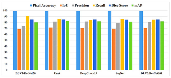
Figure 9.
The evaluation metrics of the core models for dataset1.

Figure 10.
The losses and iterations/sec of the core models for dataset1.
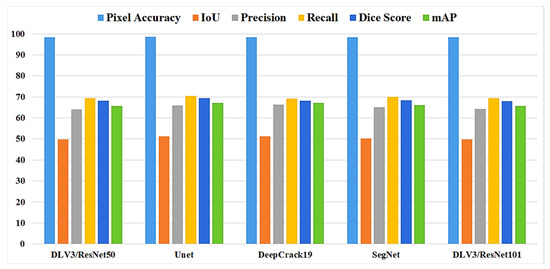
Figure 11.
The evaluation metrics of the core models for dataset2.

Figure 12.
The losses and iterations/sec of the core models for dataset2.
4.2. Performances of Co-CrackSegment
As it was mentioned in Section 3.7, the Co-CrackSegment took advantage of group learning via developing an iterative approach based on optimal evaluation metrics. The five trained deep learning semantic segmentation models were used as core models inside the Co-CrackSegment. Thereafter, the Co-CrackSegment was executed via considering five frameworks using the optimal Dice score (Co-CrackSegment/Dice), optimal IoU (Co-CrackSegment/IoU), optimal pixel accuracy (Co-CrackSegment/Pixel_Acc), optimal precision (Co-CrackSegment/Precision), and optimal recall (Co-CrackSegment/Recall). The evaluation results of the Co-CrackSegment paradigms are presented in two styles as in Table 4 and Table 5 as well as Figure 13 and Figure 14 for dataset1 and dataset2, respectively. By studying the results, the Co-CrackSegment/Dice and Co-CrackSegment/IoU have shown the best trade-off scores compared with other Co-CrackSegment frameworks. In addition, when compared with the weighted average method, most Co-CrackSegment frameworks outperformed the weighted average ensemble by means of all evaluation metrics. This is because the traditional weighted average ensemble learning for pixel-level semantic segmentation suffers from pixel blurring of crack boundaries due to average predictions resulting in high bias of predicted crack map than the ground truth. Furthermore, when comparing the results of core models with the Co-CrackSegment frameworks, it is clear that the group learning approach boosted the performance of the individual models by means of all evaluation metrics. This proved the efficiency of the Co-CrackSegment approach for the pixel-level semantic segmentation of surface cracks.
Table 4.
Segmentation metrics of the ensemble models using dataset1 (bold values indicate best performance metrics).
Table 5.
Segmentation metrics of the ensemble models using dataset2 (bold values indicate best performance metrics).
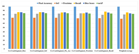
Figure 13.
The evaluation metrics of the Co-CrackSegment frameworks for dataset1.
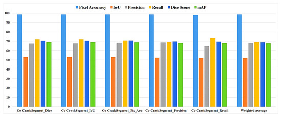
Figure 14.
The evaluation metrics of the Co-CrackSegment frameworks for dataset2.
4.3. Visual Comparison and Discussion
To give a better overview on the developed Co-CrackSegment approach, a detailed visual comparison between the different Co-CrackSegment frameworks as well as the core models is given in this section. Two groups of image samples from the DeepCrack and Rissbilder datasets were tested, as shown in Figure 15 and Figure 16, respectively. The image sample groups contained several challenging aspects. The test group1 contained eight samples, in which test sample 1 contained a wide discontinued crack with an augmentation feature at the end of it.
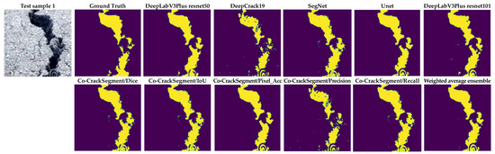
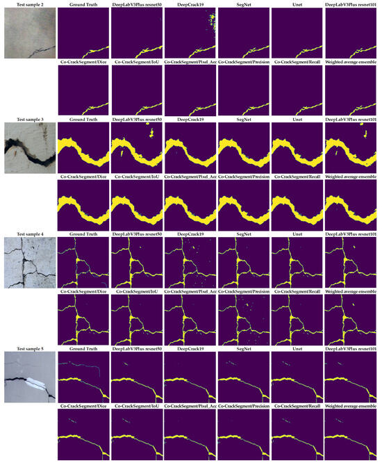
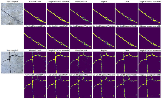
Figure 15.
Visual evaluation of the compared models using image samples of dataset 1.
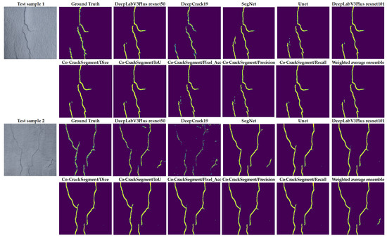
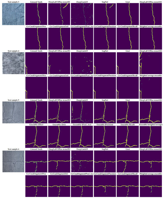
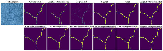
Figure 16.
Visual evaluation of the compared models using image samples of dataset 2.
From Figure 15, it can be seen that the most reduced noise and closest crack map to ground truth was achieved by the Co-CrackSegment/Pixel_Acc in the case of test sample 1. Test sample 2 contained a thin lateral crack with a blurry background which made the pixel-level identification challenging. Nevertheless, all the Co-CrackSegment frameworks achieved a very close crack map to the ground truth. Test sample 3 contained a wide crack with two challenging spots above and beneath. However, all the Co-CrackSegment methods achieved very good matches with the ground truth image, eliminating the background challenging spots. Image sample 4 contained a thin spalling with small voids in the background which contributed to the highly noisy background. Except for the tiny crack portion in the bottom-left corner, it can be seen that the Co-CrackSegment/Dice and Co-CrackSegment/IoU provided the best crack map images. Image sample 5 contained one wide crack with a repaired part in the middle as well as a very thin crack above it. It can be seen from the results that the Co-CrackSegment/Dice and Co-CrackSegment/IoU as well as Co-CrackSegment/Recall achieved the best crack maps compared with other methods. Test sample 6 included a transverse crack with a complex-colored background and scaling in addition to bulges in the middle. It was reported that the Co-CrackSegment/Dice and Co-CrackSegment/IoU as well as Co-CrackSegment/Precision achieved the best crack maps compared with other methods. In test sample 7, spalling cracks were distributed along the image with some voids in the background and very thin cracks around the main crack and the lower left part of the image. It was observed that all the Co-CrackSegment methods achieved relatively good crack maps with a trade-off between the elimination of background voids and the thin crack portions.
As shown in Figure 16, test sample 1 had three main cracks with thin ends. It was observed that the Co-CrackSegment/Dice and Co-CrackSegment/IoU as well as Co-CrackSegment/Recall achieved the best reduced noise and closet matches to original ground truth. Test sample 2 contained two main cracks with a crack-like scaling at the left side. It was reported that the Co-CrackSegment/Dice and Co-CrackSegment/IoU delivered better crack maps compared with other models, with the main advantage of reduced noise in the background. Test sample 3 contained a very thin vertical crack with scales in the background. It was reported that all the Co-CrackSegment as well as the weighted average successfully eliminated the scaling positions and accurately located the crack area. In test sample 4, only very minor lateral crack with complex color of the background and scaling like spots. Nevertheless, all the Co-CrackSegment methods achieved very good matches with the ground truth image eliminating the background challenging spots. In test sample 5, a spalling crack can be seen in the lower part of the image with a vertical crack along the image and a scaling region in the background. It can be seen that the Co-CrackSegment/Dice, Co-CrackSegment/IoU, and Co-CrackSegment/Pixel_Acc of the weighted average models delivered the best crack maps compared with the original image and the ground truth. In test sample 6, a horizontal crack with an interconnected vertical crack can be observed as well complex crack-like scaling in the background. It was reported that the CrackSegment/Dice, Co-CrackSegment/IoU, and Co-CrackSegment/Pixel_Acc also gave the best crack maps compared with the original image and ground truth. In test sample 7, a very thin crack tree with complex color and illumination of the background as well as crack-like scaling can be observed. All the Co-CrackSegment models and weighted average delivered very excellent pixel-level segmentation of the crack, except the Co-CrackSegment/Recall that misclassified the pixel of the crack-like scaling. Finally, it is clear that the Co-CrackSegment/Dice and Co-CrackSegment/IoU frameworks achieved the best performance compared with other Co-CrackSegment frameworks and the weighted average method. This confirms the results presented in the previous discussion.
It is important to note that the test samples were randomly chosen image samples with very challenging feature maps. This cannot fully reflect the overall model performances that can be better observed from the statistical results. However, it can assist to provide a better visual analysis of the pixel-level crack segmentation performances when the models are fed with complex and challenging images.
4.4. Further Comparison and Discussion Using Image Processing and Modern Evaluation Metrics
In this discussion, the following image processing and restoration metrics are utilized to assess the different segmentation predictions and compare them with the original ground truth as
- Mean squared error (MSE) [69] is a metric that is mainly utilized to compute the average squared difference between the original ground truth (OGT) and the semantic segmentation prediction (SSP) and is given as follows:
- Normalized cross-correlation (NCC) [70] is another metric of similarity between the OGT and SSP images. It calculates the similarity based on the displacement of one image relative to the other one. It can be formulated as in Equation (23) shows.
- Structural Similarity Index Measure (SSIM) [71,72] evaluates three main image characteristics: illumination, contrast, and structure. In terms of these three factors, SSIM calculates the similarity between SSP and OGT images in order to select the model with the highest SSIM score. SSIM is computed as follows:
- Peak signal to noise ratio (PSNR) [73] is another well-known metric to compute the similarity between the produced and the ground truth image. However, PSNR focuses only on the absolute error between corresponding pixels of the SSP and OGT images as illustrated in Equation (25).
- Hausdorff distance (HD) [74,75] originally computes the largest distance between two sets. For our mission, HD computed the similarity between different corresponding curves (edges) of the SSP and OGT images via calculating the maximum distance of a set of pixels in the first image to the nearest point (pixel) in the other image. It can be formulated as follows:
- Fréchet Distance (FD) is another similarity metric that focuses on curves similarity and takes into consideration the location and ordering of the curve’s points of both compared images.
Giving two edges (curves) of SSP and OGT images: A(t) and B(t), with t ϵ [0,1], FD is computed as follows [76]:
where, are parameterization factors of the interval [0,1] to establish the matching between SSP and OGT curves, d is the distance between two points of the corresponding curves at a specific time t. As in HD, low values of FD metric indicate more similarity. Cost refers to the cost of matching pairs of curves and can be calculated as follows [76]:
In order to provide a clearer picture about the performance of the developed method, four randomly selected samples from dataset 1, namely test samples 1, 3, 4, and 7 in Figure 15 and four randomly selected samples from dataset 2, namely test samples 1, 2, 4, and 5 in Figure 16, are tested. Results of the comparison are shown in Table 6 and Table 7 for dataset1 and dataset2, respectively. Where, MSE is the mean squared error, NCC is the normalized cross-correlation, SSIM is the structural similarity index, PSNR is the peak signal to noise rate, HD is the Hausdorff distance, FD is the Frechet distance. CCAcc is the Co-CrackSegment/Accuracy, CCDice is the Co-CrackSegment/Dice, CCIoU is the Co-CrackSegment/IoU, CCPrec is the Co-CrackSegment/Precision, CCRec is the Co-CrackSegment/Reall, and EWA is the ensemble weighted average. Moreover, the heatmaps across images of selected samples of datasets 1 and 2 are drawn in Figure 17 and Figure 18, respectively.
Table 6.
Comparison using image processing and modern evaluation metrics for samples of dataset 1 (bold values indicate best performance metrics).
Table 7.
Comparison using image processing and modern evaluation metrics for samples of dataset 2 (bold values indicate best performance metrics).

Figure 17.
The heatmaps of metrics across sample images of dataset1.
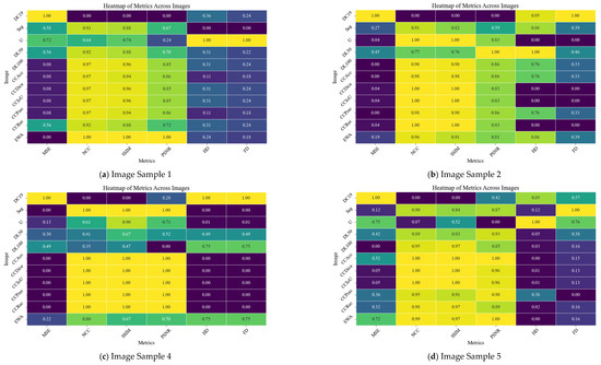
Figure 18.
The heatmaps of metrics across sample images of dataset2.
When studying Figure 17 and Table 6, and in the case of MSE, Hausdorff distance, and Frechet distance, the lower values indicate better performance, whereas in terms of SSIM, NCC, and PSNR, the higher values are better. Through analyzing the numerical study, it was observed that the proposed Co-CrackSegment ensemble models and weighted average ensemble succeed to register high SSIM, NCC, and PSNR values. On the other hand, they registered low values for HD, FD, and MSE. Some individual models achieved good numerical results in some samples, while they failed in others. For example, the SegNet model produced the best NCC, SSIM, and PSNR values for test sample 4, but failed in other test samples. However, the Unet model registered the best individual model’s metrics. In terms of Hausdorff distance, the Co-CrackSegment/Recall and weighted average ensemble showed the best results. This is normal since the Co-CrackSegment/Recall is based on merging models predictions taking into account minimizing the false negative errors which take more pixels of the required ROI of the ground truth. However, the traditional weighted average ensemble learning for pixel-level semantic segmentation suffer from pixel blurring of crack boundaries due to average predictions. Co-CrackSegment/Recall was also better in terms of Hausdorff distance since it maximized the distances between the point of the ground truth and all other similar ones in the corresponding prediction. Since Frechet distance computed the similarity between curves of the ground truth and prediction in terms of ordering along boundaries, the best models that achieve the minimum Frechet distance preserved the structural integrity and topology of the original ground truth (Co-CrackSegment/Recall, Co-CrackSegment/Precision, and Co-CrackSegment/Accuracy registered low (good) values of this metric in the test examples. In addition, when studying Figure 18 and Table 7, all metrics tended to be better in the case of using ensemble models.
It is important to note that the test samples were randomly chosen image samples with very challenging feature maps. This cannot fully reflect the overall model performances that can be better observed from the statistical results. However, it can assist to provide a better analysis of pixel-level crack segmentation performances when the models are fed with complex and challenging images.
5. Conclusions
In this research, a novel collaborative deep learning approach called Co-CrackSegment for the purpose of surface crack semantic segmentation was proposed. For the purpose of constructing the Co-CrackSegment, five core models, namely the DeepLabV3/ResNet50, U-net, DeepCrack19, SegNet, and DeepLabV3/ResNet101, were trained using two different datasets. Subsequently, the Co-CrackSegment was tested by taking into account five frameworks using the optimal Dice score (Co-CrackSegment/Dice), optimal IoU (Co-CrackSegment/IoU), optimal pixel accuracy (Co-CrackSegment/Pixel_Acc), optimal precision (Co-CrackSegment/Precision), and optimal recall (Co-CrackSegment/Recall). Comparisons were made between the core models and the different Co-CrackSegment frameworks using the tabulated and visual aspects. Furthermore, challenging test images with complex patterns were chosen to perform visual comparisons between both the core models and the developed Co-CrackSegment models. The overall findings of this paper can be summarized as follows:
- Under the theme of the core models, it has been reported that the U-net achieved a prominent performance by means of loss, pixel accuracy, IoU, Dice, and mAP when trained using dataset1. It was also observed that the DLV3/ResNet50 and DLV3/ResNet101 had achieved high performances when compromising the overall evaluation metrics. Moreover, the iteration per second score of the DeepCrack19 gave it competitive advantages as a computationally efficient model. Moreover, when trained using dataset2 and similar to dataset1, the U-net also achieved an outstanding performance by means of loss, accuracy, IoU, recall, Dice, and mAP. Also, the DeepCrack19 showed better computational performance than the other models when considering the number of iterations per seconds.
- When studying the proposed collaborative semantic segmentation Co-CrackSegment approach, the Co-CrackSegment/Dice and Co-CrackSegment/IoU showed the best trade-off evaluation scores compared with other Co-CrackSegment frameworks. Furthermore, when compared with the weighted average method, most Co-CrackSegment frameworks outperformed the weighted average ensemble as well as the core models by means of all evaluation metrics. This was because the traditional weighted average ensemble learning for pixel-level semantic segmentation suffered from pixel blurring of the crack boundaries due to average predictions resulting in high bias of the predicted crack map than the ground truth. Furthermore, when comparing the results of core models with the Co-CrackSegment frameworks, it was observed that the collaborative learning approach had boosted the performance of the individual models by means of all evaluation metrics. This proved the efficiency of the Co-CrackSegment approach for pixel-level semantic segmentation of surface cracks.
- When studying feeding the developed models with test samples that contained many challenges, such as crack-like scaling, foreign objects, thin cracks, bulges, voids, spalling, etc., it was reported that all the developed Co-CrackSegment approaches for pixel-level semantic segmentation of surface cracks gave very enhanced crack maps even in challenging cases. Also, the Co-CrackSegment/Dice and Co-CrackSegment/IoU frameworks achieved the best performance compared with other Co-CrackSegment frameworks and the weighted average method as well as the core models. This confirms the results presented in the previous discussion.
- It is well-known that when developing models for the pixel-level identification of concrete cracks, it is very important to realize that cracks occupy very small parts of the images, whereas the data are overwhelmed with background pixels. In other words, in an input image with a crack, the majority of pixels belong to the background class and minority of pixels belong to the crack class. Therefore, the crack image datasets are considered as highly imbalanced when conducting pixel-level classification. Hence, even minor improvements in evaluation metrics have a significant impact on effective localization of cracks within the background. In addition, the performance metrics such as pixel accuracy, precision, recall, and IoU are sensitive to such imbalanced data, and any enhancement in those metrics of the minority class of crack pixels is considered a boost to prediction performance. The use of the ensemble model, which combines the predictions of several models, helps to tackle the pixel classes’ imbalance and enhance the segmentation accuracy. To add, in practical scenarios, even a very narrow crack can be a considered as a warning sign for greater structural damage. Hence, even a slight improvement in segmentation accuracy might be very useful for early damage detection to prevent later catastrophic events.
- The practical limitations of this study can be summarized as the computational complexity, data annotation, core model selection, generalization ability, etc. When considering the ensemble learning for the pixel-level crack identification, the training of multiple models requires more computational efforts; however, the boosted prediction accuracy of the ensemble learning can offer a sort of tolerant towards computational time. Moreover, when preparing the data for training, more efforts are required to prepare ground truth feature maps, which are required in both individual model- or ensemble learning-based semantic segmentation. Furthermore, the availability of many semantic segmentation models in the literature makes the selection of best suited core models more challenging. However, the developed method solves this problem by providing the possibility of any semantic segmentation models, even if trained using other datasets. In addition, even if the ensemble learning-based semantic segmentation models aim to improve the generalization of the prediction via leveraging several core models, any bias in core models can be forwarded to the ensemble model degrading prediction accuracy. Nevertheless, the proposed Co-CrackSegment model chooses the best prediction of the core models, rather than accumulating or averaging their prediction like the traditional average weighting ensemble.
- Finally, several future improvements can be made to improve the proposed method. Firstly, the Co-CrackSegment approach can accept the insertion of any semantic segmentation model. This is mainly due to its flexibility to add core models to its main framework. Moreover, the Co-CrackSegment method can be boosted via improving the utilized performance metrics to make a better trade-off between the original performance metrics that have already been used in its framework. Furthermore, the proposed Co-CrackSegment method can be further improved for multilevel semantic segmentation of structural surface defects. Lastly, the Co-CrackSegment can be easily adapted to be used in other semantic segmentation applications.
Supplementary Materials
The following supporting information can be downloaded at: https://www.mdpi.com/article/10.3390/math12193105/s1, Figure S1: The training-testing curves of DeepLabV3-ResNet50 for dataset1, Figure S2: The training-testing curves of U-net for dataset1, Figure S3: The training-testing curves of CrackNet19 for dataset1, Figure S4: The training-testing curves of SegNet for dataset1, Figure S5: The training-testing curves of DeepLabV3ResNet101 for dataset1, Figure S6: The training-testing curves of DeepLabV3-ResNet50 for dataset2, Figure S7: The training-testing curves of U-net for dataset2, Figure S8: The training-testing curves of CrackNet19 for dataset2, Figure S9: The training-testing curves of SegNet for dataset2, Figure S10: The training-testing curves of DeepLabV3-ResNet101 for dataset2.
Author Contributions
Conceptualization, N.F.A. and A.M.; methodology, N.F.A. and A.M.; software, N.F.A. and A.M.; validation, N.F.A., A.M., X.Z., L.S., P.G.A., Q.W. and M.C.; formal analysis, N.F.A., A.M., X.Z., L.S., P.G.A., Q.W. and M.C.; investigation, N.F.A. and A.M.; resources, N.F.A., A.M. and M.C.; data curation, N.F.A. and A.M.; writing—original draft preparation, N.F.A. and A.M.; writing—review and editing, N.F.A., A.M., Q.W. and M.C.; visualization, N.F.A., A.M., X.Z., L.S., P.G.A., Q.W. and M.C.; supervision, N.F.A., A.M., X.Z., L.S., P.G.A., Q.W. and M.C.; project administration, N.F.A., A.M., X.Z., L.S., P.G.A., Q.W. and M.C.; funding acquisition, N.F.A., A.M., X.Z., L.S., P.G.A., Q.W. and M.C. All authors have read and agreed to the published version of the manuscript.
Funding
This work was supported by the Research Fund for International Young Scientists of the National Natural Science Foundation of China (No. 52250410359), the Natural Science Research Start-up Foundation of Recruiting Talents of Nanjing University of Posts and Telecommunications (No. NY223176), the 2022 National Young Foreign Talents Program of China (No. QN2022143002L), and the Jiangsu-Czech Bilateral Co-funding R&D Project (No. BZ2023011).
Data Availability Statement
Datasets used in this work are public datasets.
Conflicts of Interest
The authors declare no conflicts of interest.
References
- Alkayem, N.F.; Cao, M.; Zhang, Y.; Bayat, M.; Su, Z. Structural damage detection using finite element model updating with evolutionary algorithms: A survey. Neural Comput. Appl. 2018, 30, 389–411. [Google Scholar] [CrossRef] [PubMed]
- Nguyen, S.D.; Tran, T.S.; Tran, V.P.; Lee, H.J.; Piran, M.J.; Le, V.P. Deep Learning-Based Crack Detection: A Survey. Int. J. Pavement Res. Technol. 2023, 16, 943–967. [Google Scholar] [CrossRef]
- Bhatt, P.M.; Malhan, R.K.; Rajendran, P.; Shah, B.C.; Thakar, S.; Yoon, Y.J.; Gupta, S.K. Image-Based Surface Defect Detection Using Deep Learning: A Review. J. Comput. Inf. Sci. Eng. 2021, 21, 040801. [Google Scholar] [CrossRef]
- Tapeh, A.T.G.; Naser, M.Z. Artificial Intelligence, Machine Learning, and Deep Learning in Structural Engineering: A Scientometrics Review of Trends and Best Practices. Arch. Comput. Methods Eng. 2022, 30, 115–159. [Google Scholar] [CrossRef]
- Thai, H.-T. Machine learning for structural engineering: A state-of-the-art review. Structures 2022, 38, 448–491. [Google Scholar] [CrossRef]
- Cao, M.; Alkayem, N.F.; Pan, L.; Novák, D. Advanced methods in neural networks-based sensitivity analysis with their applications in civil engineering. In Artificial Neural Networks: Models and Applications; IntechOpen: Rijeka, Croatia, 2016. [Google Scholar]
- Nguyen, D.H.; Wahab, M.A. Damage detection in slab structures based on two-dimensional curvature mode shape method and Faster R-CNN. Adv. Eng. Softw. 2023, 176, 103371. [Google Scholar] [CrossRef]
- Yu, L.; He, S.; Liu, X.; Jiang, S.; Xiang, S. Intelligent Crack Detection and Quantification in the Concrete Bridge: A Deep Learning-Assisted Image Processing Approach. Adv. Civ. Eng. 2022, 2022, 1813821. [Google Scholar] [CrossRef]
- Kaewniam, P.; Cao, M.; Alkayem, N.F.; Li, D.; Manoach, E. Recent advances in damage detection of wind turbine blades: A state-of-the-art review. Renew. Sustain. Energy Rev. 2022, 167, 112723. [Google Scholar] [CrossRef]
- Wang, S.-J.; Zhang, J.-K.; Lu, X.-Q. Research on Real-Time Detection Algorithm for Pavement Cracks Based on SparseInst-CDSM. Mathematics 2023, 11, 3277. [Google Scholar] [CrossRef]
- Yu, G.; Zhou, X. An Improved YOLOv5 Crack Detection Method Combined with a Bottleneck Transformer. Mathematics 2023, 11, 2377. [Google Scholar] [CrossRef]
- Tran, T.S.; Nguyen, S.D.; Lee, H.J.; Tran, V.P. Advanced crack detection and segmentation on bridge decks using deep learning. Constr. Build. Mater. 2023, 400, 132839. [Google Scholar] [CrossRef]
- Zhang, J.; Cai, Y.-Y.; Yang, D.; Yuan, Y.; He, W.-Y.; Wang, Y.-J. MobileNetV3-BLS: A broad learning approach for automatic concrete surface crack detection. Constr. Build. Mater. 2023, 392, 131941. [Google Scholar] [CrossRef]
- Alkayem, N.F.; Shen, L.; Mayya, A.; Asteris, P.G.; Fu, R.; Di Luzio, G.; Strauss, A.; Cao, M. Prediction of concrete and FRC properties at high temperature using machine and deep learning: A review of recent advances and future perspectives. J. Build. Eng. 2024, 83, 108369. [Google Scholar] [CrossRef]
- Fu, R.; Cao, M.; Novák, D.; Qian, X.; Alkayem, N.F. Extended efficient convolutional neural network for concrete crack detection with illustrated merits. Autom. Constr. 2023, 156, 105098. [Google Scholar] [CrossRef]
- Xiong, C.; Zayed, T.; Abdelkader, E.M. A novel YOLOv8-GAM-Wise-IoU model for automated detection of bridge surface cracks. Constr. Build. Mater. 2024, 414, 135025. [Google Scholar] [CrossRef]
- Alkayem, N.F.; Cao, M.; Ragulskis, M. Damage Diagnosis in 3D Structures Using a Novel Hybrid Multiobjective Optimization and FE Model Updating Framework. Complexity 2018, 2018, 3541676. [Google Scholar] [CrossRef]
- Cao, M.; Qiao, P.; Ren, Q. Improved hybrid wavelet neural network methodology for time-varying behavior prediction of engineering structures. Neural Comput. Appl. 2009, 18, 821–832. [Google Scholar] [CrossRef]
- Alkayem, N.F.; Cao, M. Damage identification in three-dimensional structures using single-objective evolutionary algorithms and finite element model updating: Evaluation and comparison. Eng. Optim. 2018, 50, 1695–1714. [Google Scholar] [CrossRef]
- Arafin, P.; Billah, A.M.; Issa, A. Deep learning-based concrete defects classification and detection using semantic segmentation. Struct. Health Monit. 2023, 23, 383–409. [Google Scholar] [CrossRef]
- Hang, J.; Wu, Y.; Li, Y.; Lai, T.; Zhang, J.; Li, Y. A deep learning semantic segmentation network with attention mechanism for concrete crack detection. Struct. Health Monit. 2023, 22, 3006–3026. [Google Scholar] [CrossRef]
- Tabernik, D.; Šuc, M.; Skočaj, D. Automated detection and segmentation of cracks in concrete surfaces using joined segmentation and classification deep neural network. Constr. Build. Mater. 2023, 408, 133582. [Google Scholar] [CrossRef]
- Shang, J.; Xu, J.; Zhang, A.A.; Liu, Y.; Wang, K.C.; Ren, D.; Zhang, H.; Dong, Z.; He, A. Automatic Pixel-level pavement sealed crack detection using Multi-fusion U-Net network. Measurement 2023, 208, 112475. [Google Scholar] [CrossRef]
- Chen, B.; Zhang, H.; Wang, G.; Huo, J.; Li, Y.; Li, L. Automatic concrete infrastructure crack semantic segmentation using deep learning. Autom. Constr. 2023, 152, 104950. [Google Scholar] [CrossRef]
- Dang, L.M.; Wang, H.; Li, Y.; Nguyen, L.Q.; Nguyen, T.N.; Song, H.-K.; Moon, H. Lightweight pixel-level semantic segmentation and analysis for sewer defects using deep learning. Constr. Build. Mater. 2023, 371, 130792. [Google Scholar] [CrossRef]
- Joshi, D.; Singh, T.P.; Sharma, G. Automatic surface crack detection using segmentation-based deep-learning approach. Eng. Fract. Mech. 2022, 268, 108467. [Google Scholar] [CrossRef]
- Mishra, M.; Jain, V.; Singh, S.K.; Maity, D. Two-stage method based on the you only look once framework and image segmentation for crack detection in concrete structures. Arch. Struct. Constr. 2022, 3, 429–446. [Google Scholar] [CrossRef]
- Shi, P.; Shao, S.; Fan, X.; Zhou, Z.; Xin, Y. MCL-CrackNet: A Concrete Crack Segmentation Network Using Multilevel Contrastive Learning. IEEE Trans. Instrum. Meas. 2023, 72, 5030415. [Google Scholar] [CrossRef]
- Savino, P.; Tondolo, F. Civil infrastructure defect assessment using pixel-wise segmentation based on deep learning. J. Civ. Struct. Health Monit. 2022, 13, 35–48. [Google Scholar] [CrossRef]
- Hadinata, P.N.; Simanta, D.; Eddy, L.; Nagai, K. Multiclass Segmentation of Concrete Surface Damages Using U-Net and DeepLabV3+. Appl. Sci. 2023, 13, 2398. [Google Scholar] [CrossRef]
- Al-Huda, Z.; Peng, B.; Algburi, R.N.A.; Al-Antari, M.A.; Al-Jarazi, R.; Zhai, D. A hybrid deep learning pavement crack semantic segmentation. Eng. Appl. Artif. Intell. 2023, 122, 106142. [Google Scholar] [CrossRef]
- Ali, R.; Chuah, J.H.; Abu Talip, M.S.; Mokhtar, N.; Shoaib, M.A. Automatic pixel-level crack segmentation in images using fully convolutional neural network based on residual blocks and pixel local weights. Eng. Appl. Artif. Intell. 2021, 104, 104391. [Google Scholar] [CrossRef]
- Kang, D.; Benipal, S.S.; Gopal, D.L.; Cha, Y.-J. Hybrid pixel-level concrete crack segmentation and quantification across complex backgrounds using deep learning. Autom. Constr. 2020, 118, 103291. [Google Scholar] [CrossRef]
- Sha, C.; Yue, C.; Wang, W. Ensemble 1D DenseNet Damage Identification Method Based on Vibration Acceleration. Struct. Durab. Health Monit. 2023, 17, 369–381. [Google Scholar] [CrossRef]
- Kailkhura, V.; Aravindh, S.; Jha, S.S.; Jayanth, N. Ensemble learning-based approach for crack detection using CNN. In Proceedings of the Fourth International Conference on Trends in Electronics and Informatics (ICOEI 2020), Tirunelveli, India, 15–17 June 2020. [Google Scholar]
- Liao, Y.; Huang, C.; Yin, Y. Segmentation of Apparent Multi-Defect Images of Concrete Bridges Based on PID Encoder and Multi-Feature Fusion. Buildings 2024, 14, 1463. [Google Scholar] [CrossRef]
- Hong, Y.; Yoo, S.B. OASIS-Net: Morphological Attention Ensemble Learning for Surface Defect Detection. Mathematics 2022, 10, 4114. [Google Scholar] [CrossRef]
- Barkhordari, M.S.; Armaghani, D.J.; Asteris, P.G. Structural Damage Identification Using Ensemble Deep Convolutional Neural Network Models. Comput. Model. Eng. Sci. 2023, 134, 835–855. [Google Scholar] [CrossRef]
- Maarouf, A.A.; Hachouf, F. Transfer Learning-based Ensemble Deep Learning for Road Cracks Detection. In Proceedings of the International Conference on Advanced Aspects of Software Engineering (ICAASE), Constantine, Algeria, 17–18 September 2022. [Google Scholar]
- Bousselham, W.; Thibault, G.; Pagano, L.; Machireddy, A. Efficient Self-Ensemble for Semantic Segmentation. arXiv 2022, arXiv:cs.CV/2111.13280. [Google Scholar]
- Nigam, I.; Huang, C.; Ramanan, D. Ensemble Knowledge Transfer for Semantic Segmentation. In Proceedings of the IEEE Winter Conference on Applications of Computer Vision, Lake Tahoe, NV, USA, 12–15 March 2018. [Google Scholar]
- Zhang, L.; Slade, S.; Lim, C.P.; Asadi, H.; Nahavandi, S.; Huang, H.; Ruan, H. Semantic segmentation using Firefly Algorithm-based evolving ensemble deep neural networks. Knowl.-Based Syst. 2023, 277, 110828. [Google Scholar] [CrossRef]
- Lee, C.; Yoo, S.; Kim, S.; Lee, J. Progressive Weighted Self-Training Ensemble for Multi-Type Skin Lesion Semantic Segmentation. IEEE Access 2022, 10, 132376–132383. [Google Scholar] [CrossRef]
- Lee, T.; Kim, J.-H.; Lee, S.-J.; Ryu, S.-K.; Joo, B.-C. Improvement of Concrete Crack Segmentation Performance Using Stacking Ensemble Learning. Appl. Sci. 2023, 13, 2367. [Google Scholar] [CrossRef]
- Li, S.; Zhao, X. A Performance Improvement Strategy for Concrete Damage Detection Using Stacking Ensemble Learning of Multiple Semantic Segmentation Networks. Sensors 2022, 22, 3341. [Google Scholar] [CrossRef] [PubMed]
- Amieghemen, G.E.; Sherif, M.M. Deep convolutional neural network ensemble for pavement crack detection using high elevation UAV images. Struct. Infrastruct. Eng. 2023, 1–16. [Google Scholar] [CrossRef]
- Cyganov, G.; Rychenkov, A.; Sinitca, A.; Kaplun, D. Using the fuzzy integrals for the ensemble-based segmentation of asphalt cracks. Ind. Artif. Intell. 2023, 1, 5. [Google Scholar] [CrossRef]
- Chen, Y.; Mo, Y.; Readie, A.; Ligozio, G.; Mandal, I.; Jabbar, F.; Coroller, T.; Papież, B.W. VertXNet: An ensemble method for vertebral body segmentation and identification from cervical and lumbar spinal X-rays. Sci. Rep. 2024, 14, 3341. [Google Scholar] [CrossRef] [PubMed]
- Bao, R.; Palaniappan, K.; Zhao, Y.; Seetharaman, G. GLSNet++: Global and Local-Stream Feature Fusion for LiDAR Point Cloud Semantic Segmentation Using GNN Demixing Block. IEEE Sensors J. 2024, 24, 11610–11624. [Google Scholar] [CrossRef]
- Dais, D.; Bal, I.E.; Smyrou, E.; Sarhosis, V. Automatic crack classification and segmentation on masonry surfaces using convolutional neural networks and transfer learning. Autom. Constr. 2021, 125, 103606. [Google Scholar] [CrossRef]
- Vij, R.; Arora, S. A hybrid evolutionary weighted ensemble of deep transfer learning models for retinal vessel segmentation and diabetic retinopathy detection. Comput. Electr. Eng. 2024, 115, 109107. [Google Scholar] [CrossRef]
- Fan, Z.; Li, C.; Chen, Y.; Mascio, P.D.; Chen, X.; Zhu, G.; Loprencipe, G. Ensemble of Deep Convolutional Neural Networks for Automatic Pavement Crack Detection and Measurement. Coatings 2020, 10, 152. [Google Scholar] [CrossRef]
- Devan, K.S.; Kestler, H.A.; Read, C.; Walther, P. Weighted average ensemble-based semantic segmentation in biological electron microscopy images. Histochem. 2022, 158, 447–462. [Google Scholar] [CrossRef]
- Panella, F.; Lipani, A.; Boehm, J. Semantic segmentation of cracks: Data challenges and architecture. Autom. Constr. 2022, 135, 104110. [Google Scholar] [CrossRef]
- Munawar, H.S.; Hammad, A.W.A.; Haddad, A.; Soares, C.A.P.; Waller, S.T. Image-Based Crack Detection Methods: A Review. Infrastructures 2021, 6, 115. [Google Scholar] [CrossRef]
- Zhang, L.; Li, H.; Shen, P.; Zhu, G.; Song, J.; Shah, S.A.A.; Bennamoun, M.; Zhang, L. Improving Semantic Image Segmentation With a Probabilistic Superpixel-Based Dense Conditional Random Field. IEEE Access 2018, 6, 15297–15310. [Google Scholar] [CrossRef]
- Jadon, S. A survey of loss functions for semantic segmentation. In Proceedings of the 2020 IEEE Conference on Computational Intelligence in Bioinformatics and Computational Biology (CIBCB), Viña del Mar, Chile, 27–29 October 2020; pp. 1–7. [Google Scholar]
- Milletari, F.; Navab, N.; Ahmadi, S.-A. V-net: Fully convolutional neural networks for volumetric medical image segmentation. In Proceedings of the 2016 Fourth International Conference on 3D Vision (3DV), Stanford, CA, USA, 25–28 October 2016; pp. 565–571. [Google Scholar]
- Bengio, Y.; Goodfellow, I.; Courville, A. Deep Learning; MIT Press: Cambridge, MA, USA, 2017; Volume 1. [Google Scholar]
- Gu, J.; Wang, Z.; Kuen, J.; Ma, L.; Shahroudy, A.; Shuai, B.; Liu, T.; Wang, X.; Wang, G.; Cai, J.; et al. Recent advances in convolutional neural networks. Pattern Recognit. 2018, 77, 354–377. [Google Scholar] [CrossRef]
- Zhu, H.; Miao, Y.; Zhang, X. Semantic Image Segmentation with Improved Position Attention and Feature Fusion. Neural Process. Lett. 2020, 52, 329–351. [Google Scholar] [CrossRef]
- Andriyanov, N. Using ArcFace Loss Function and Softmax with Temperature Activation Function for Improvement in X-ray Baggage Image Classification Quality. Mathematics 2024, 12, 2547. [Google Scholar] [CrossRef]
- Liu, Y.; Yao, J.; Lu, X.; Xie, R.; Li, L. DeepCrack: A deep hierarchical feature learning architecture for crack segmentation. Neurocomputing 2019, 338, 139–153. [Google Scholar] [CrossRef]
- Kulkarni, S.; Singh, S.; Balakrishnan, D.; Sharma, S.; Devunuri, S.; Korlapati, S.C.R. CrackSeg9k: A Collection and Benchmark for Crack Segmentation Datasets and Frameworks. In Computer Vision—ECCV 2022 Workshops; Karlinsky, L., Michaeli, T., Nishino, K., Eds.; Lecture Notes in Computer Science; Springer: Cham, Switzerland, 2022; Volume 13807. [Google Scholar]
- Pak, M.; Kim, S. Crack Detection Using Fully Convolutional Network in Wall-Climbing Robot. In Advances in Computer Science and Ubiquitous Computing; Park, J.J., Fong, S.J., Pan, Y., Sung, Y., Eds.; Lecture Notes in Electrical Engineering; Springer: Singapore, 2021; Volume 715. [Google Scholar]
- Ronneberger, O.; Fischer, P.; Brox, T. U-Net: Convolutional Networks for Biomedical Image Segmentation. In Medical Image Computing and Computer-Assisted Intervention—MICCAI 2015; Navab, N., Hornegger, J., Wells, W., Frangi, A., Eds.; Lecture Notes in Computer Science; Springer: Cham, Switzerland, 2015; Volume 9351. [Google Scholar]
- Simonyan, K.; Zisserman, A. Very Deep Convolutional Networks for Large-Scale Image Recognition. arXiv 2014, arXiv:1409.1556. [Google Scholar]
- Chen, L.-C.; Papandreou, G.; Schroff, F.; Adam, H. Rethinking Atrous Convolution for Semantic Image Segmentation. arXiv 2017, arXiv:1706.05587. [Google Scholar]
- Wang, Z.; Bovik, A.C. Mean squared error: Love it or leave it? A new look at Signal Fidelity Measures. IEEE Signal Process. Mag. 2009, 26, 98–117. [Google Scholar] [CrossRef]
- Almira, J.M.; Phelippeau, H.; Martinez-Sanchez, A. Fast normalized cross-correlation for template matching with rotations. J. Appl. Math. Comput. 2024, 1–33. [Google Scholar] [CrossRef]
- Setiadi, D.R.I.M. PSNR vs SSIM: Imperceptibility quality assessment for image steganography. Multimedia Tools Appl. 2020, 80, 8423–8444. [Google Scholar] [CrossRef]
- Ding, K.; Ma, K.; Wang, S.; Simoncelli, E.P. Image Quality Assessment: Unifying Structure and Texture Similarity. IEEE Trans. Pattern Anal. Mach. Intell. 2020, 44, 2567–2581. [Google Scholar] [CrossRef]
- Horé, A.; Ziou, D. Image Quality Metrics: PSNR vs. SSIM. In Proceedings of the 2010 20th International Conference on Pattern Recognition, Istanbul, Turkey, 23–26 August 2010; pp. 2366–2369. [Google Scholar] [CrossRef]
- Chen, G.; Lan, H.; Yan, Y.; Peng, Y. Similarity evaluation method of single flow point energy consumption mapping based on Fréchet distance. Meas. Sci. Technol. 2023, 34, 125011. [Google Scholar] [CrossRef]
- Kwon, Y.; Moon, J.; Chung, Y. Noise-Tolerant Trajectory Distance Computation in the Presence of Inherent Noise for Video Surveillance Applications. IEEE Access 2024, 12, 92400–92418. [Google Scholar] [CrossRef]
- Buchin, K.; Löffler, M.; Ophelders, T.; Popov, A.; Urhausen, J.; Verbeek, K. Computing the Fréchet distance between uncertain curves in one dimension. Comput. Geom. 2023, 109, 101923. [Google Scholar] [CrossRef]
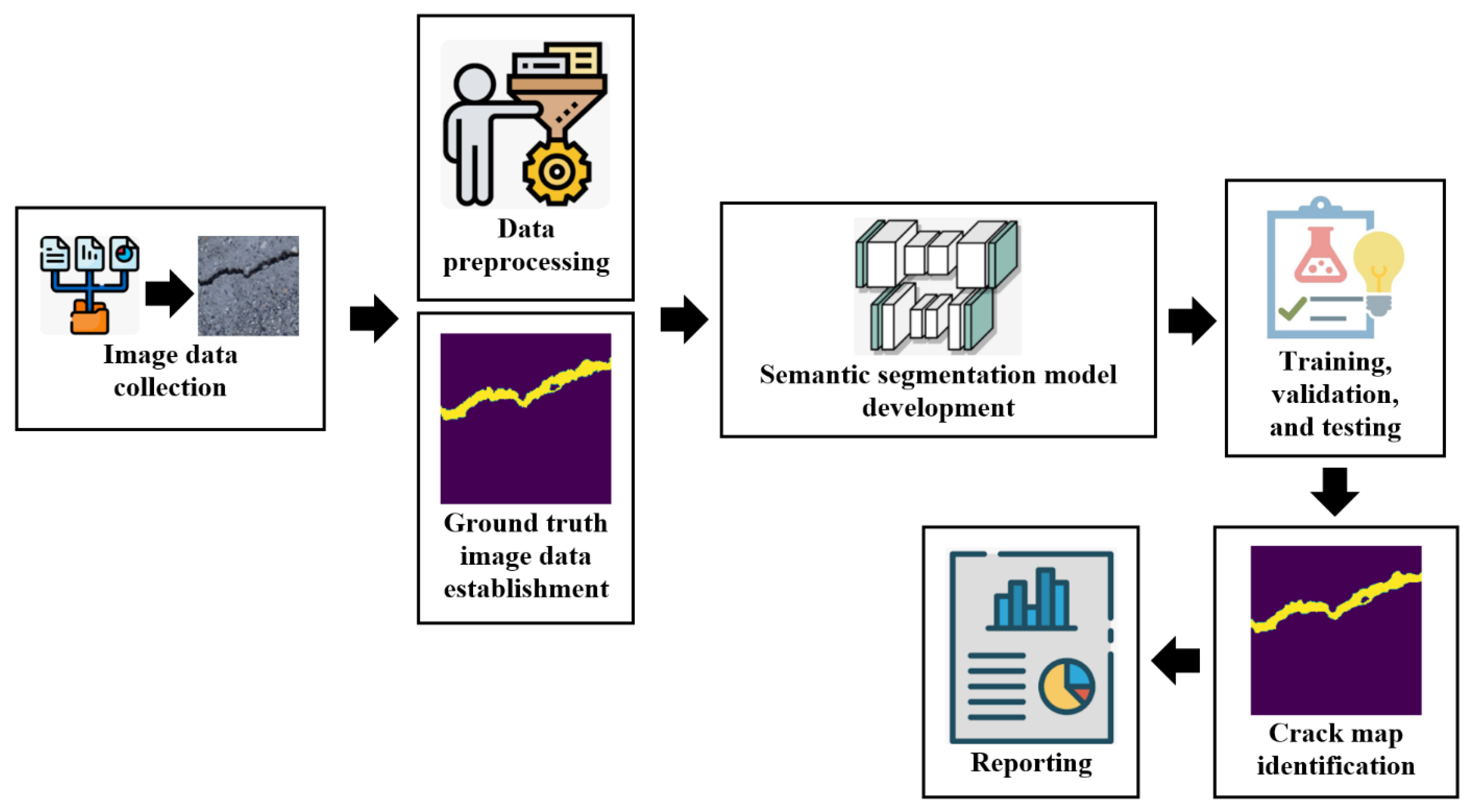
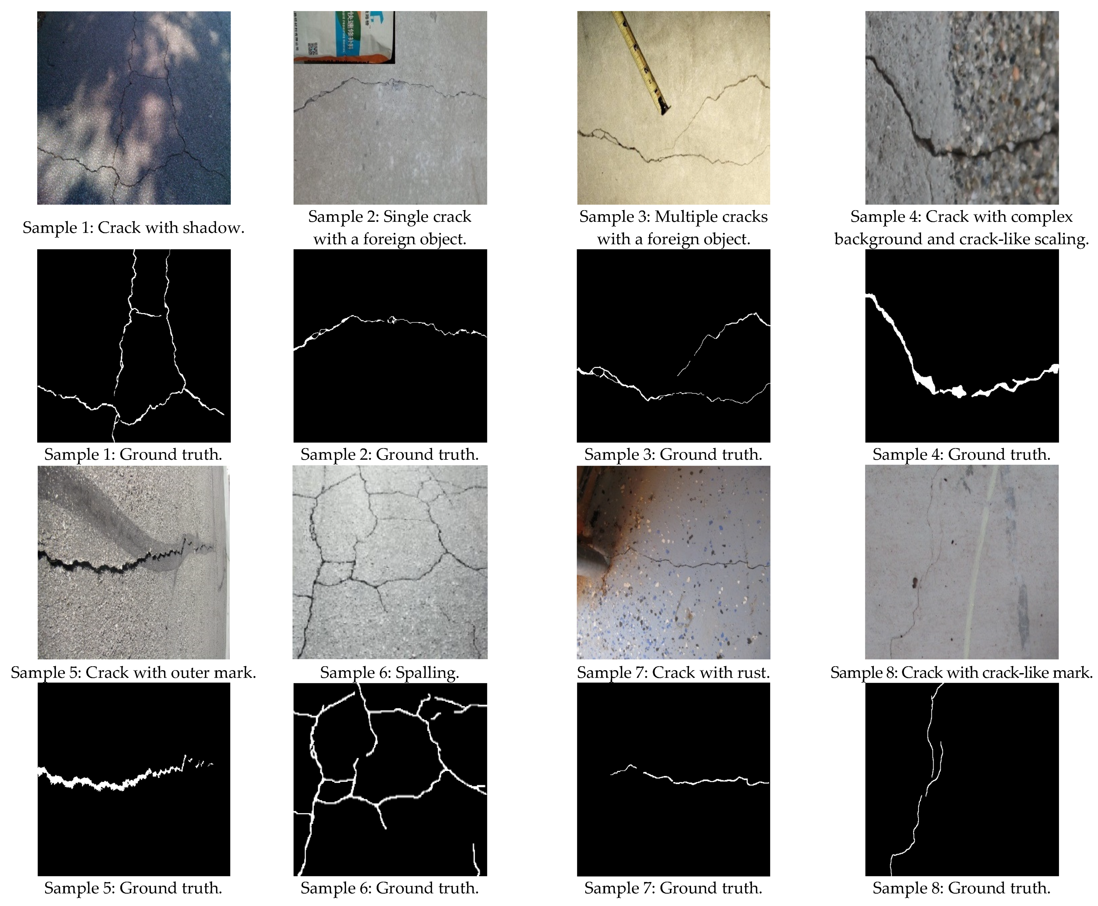


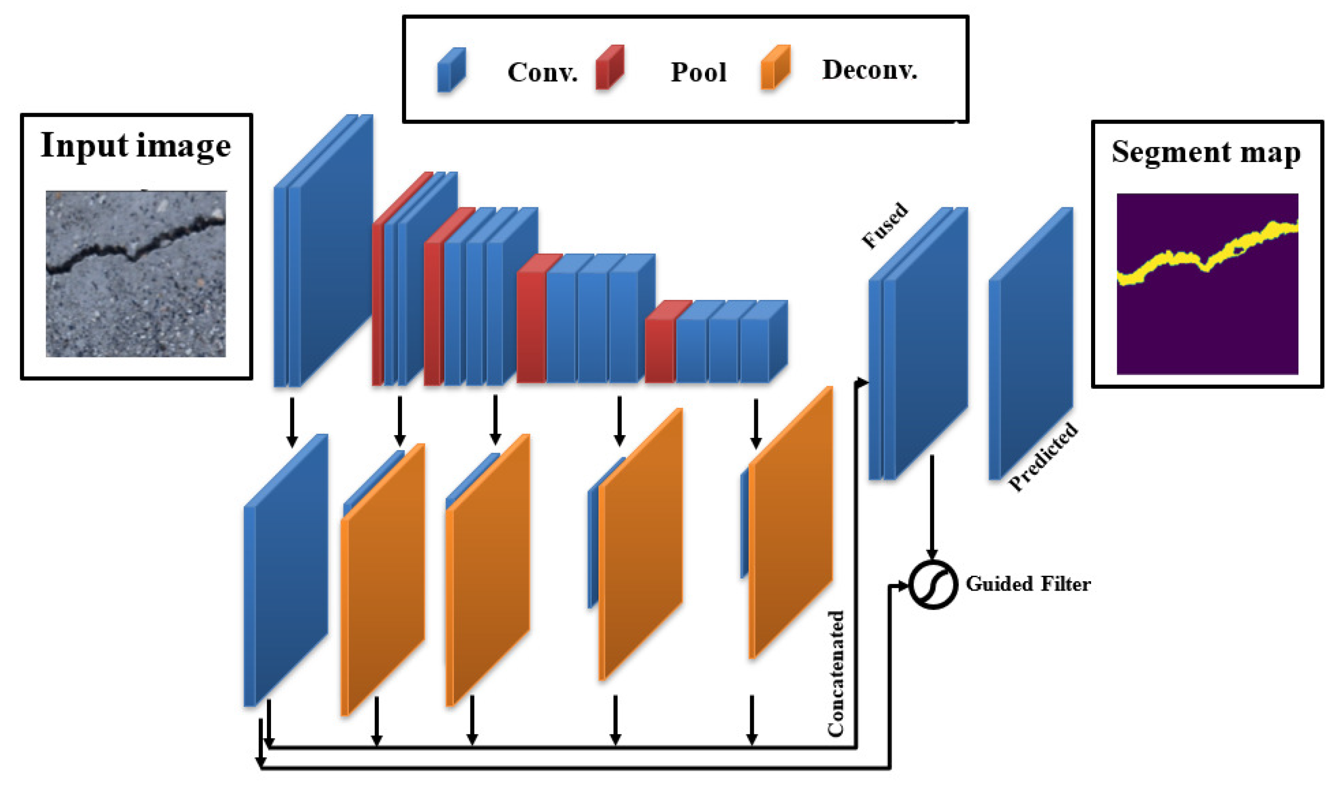

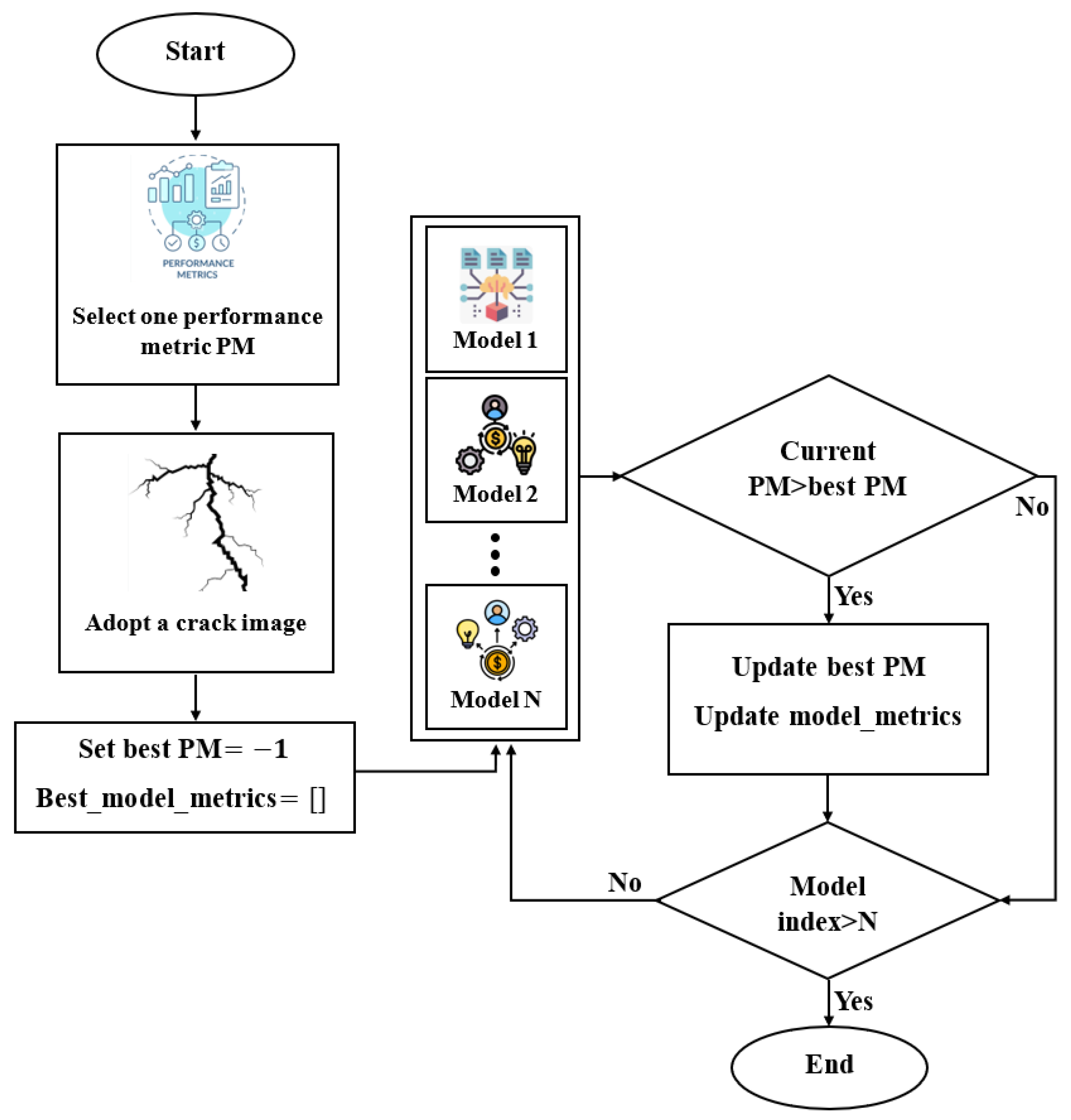
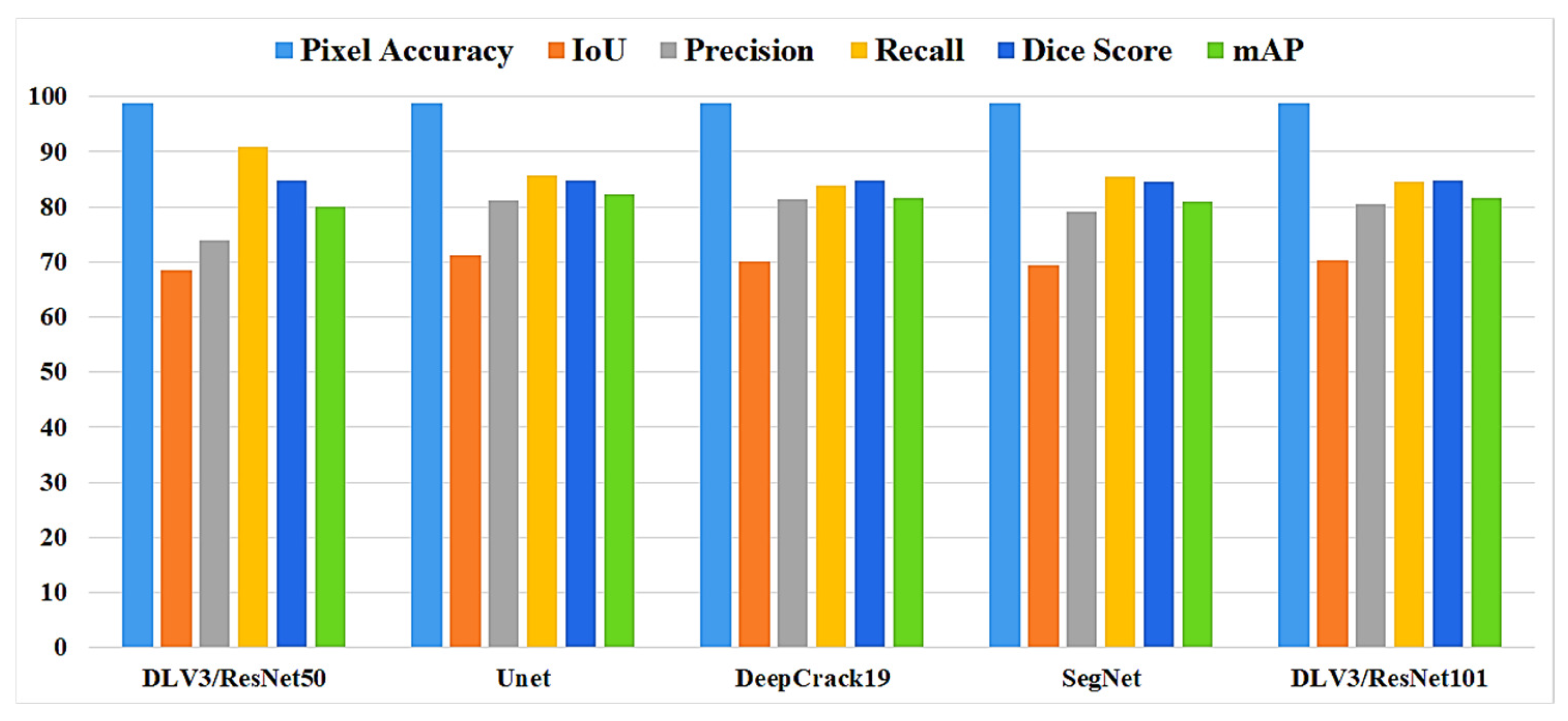
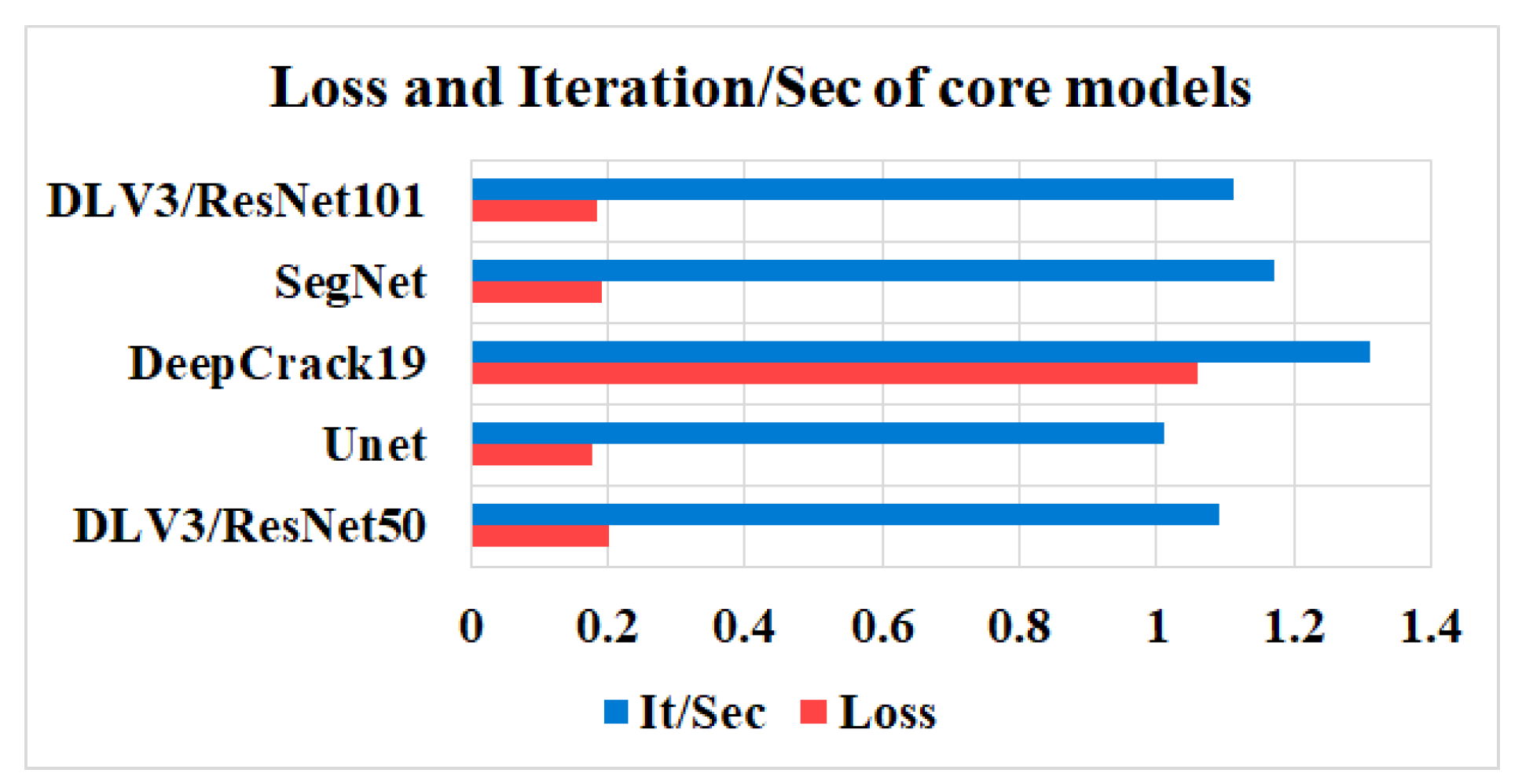

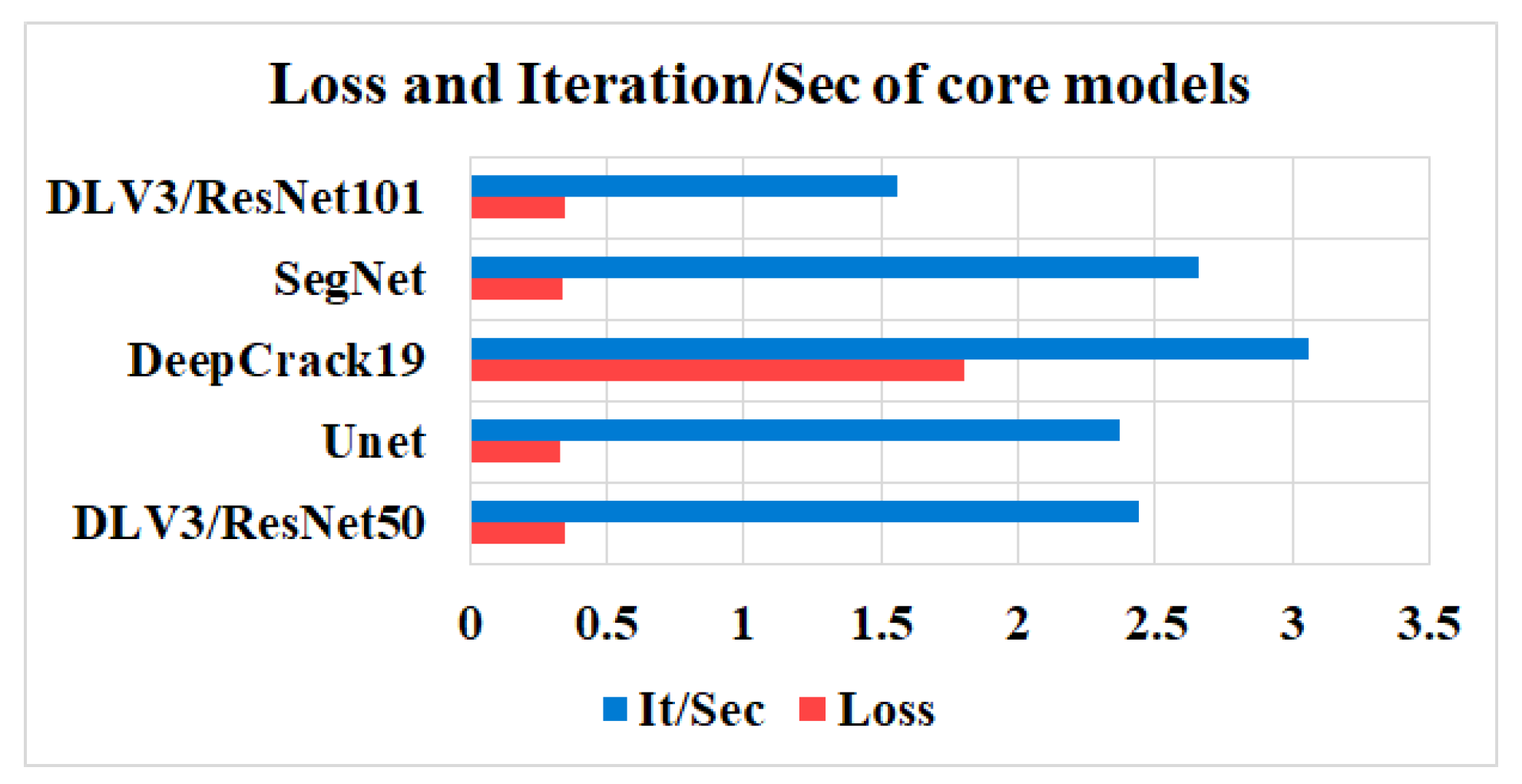


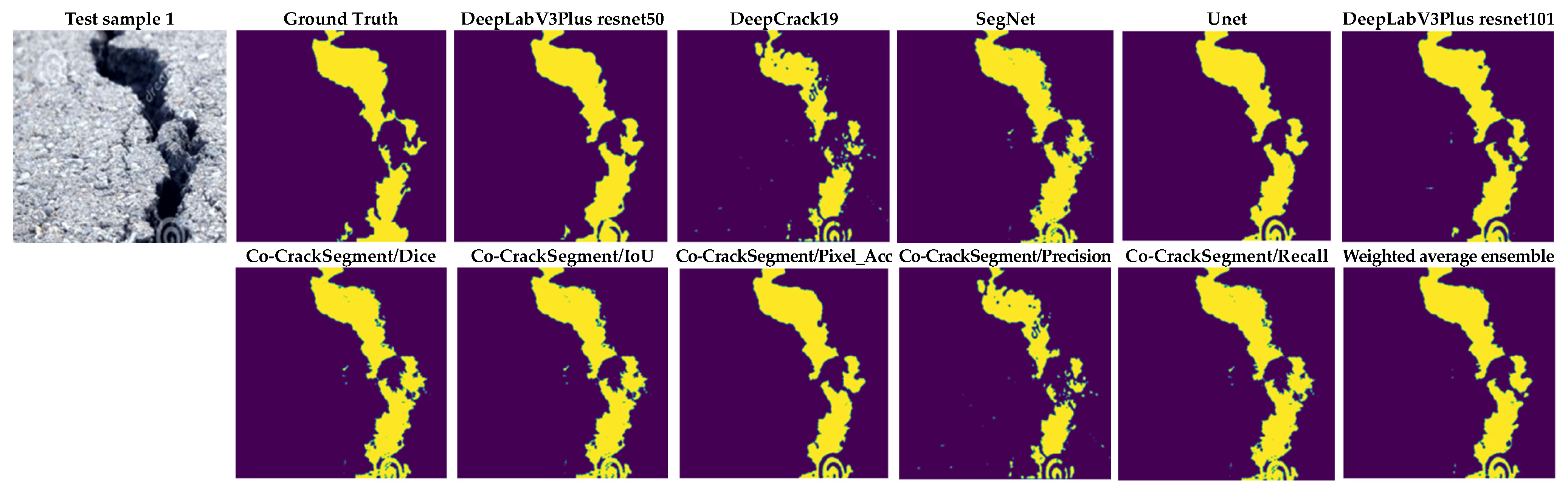
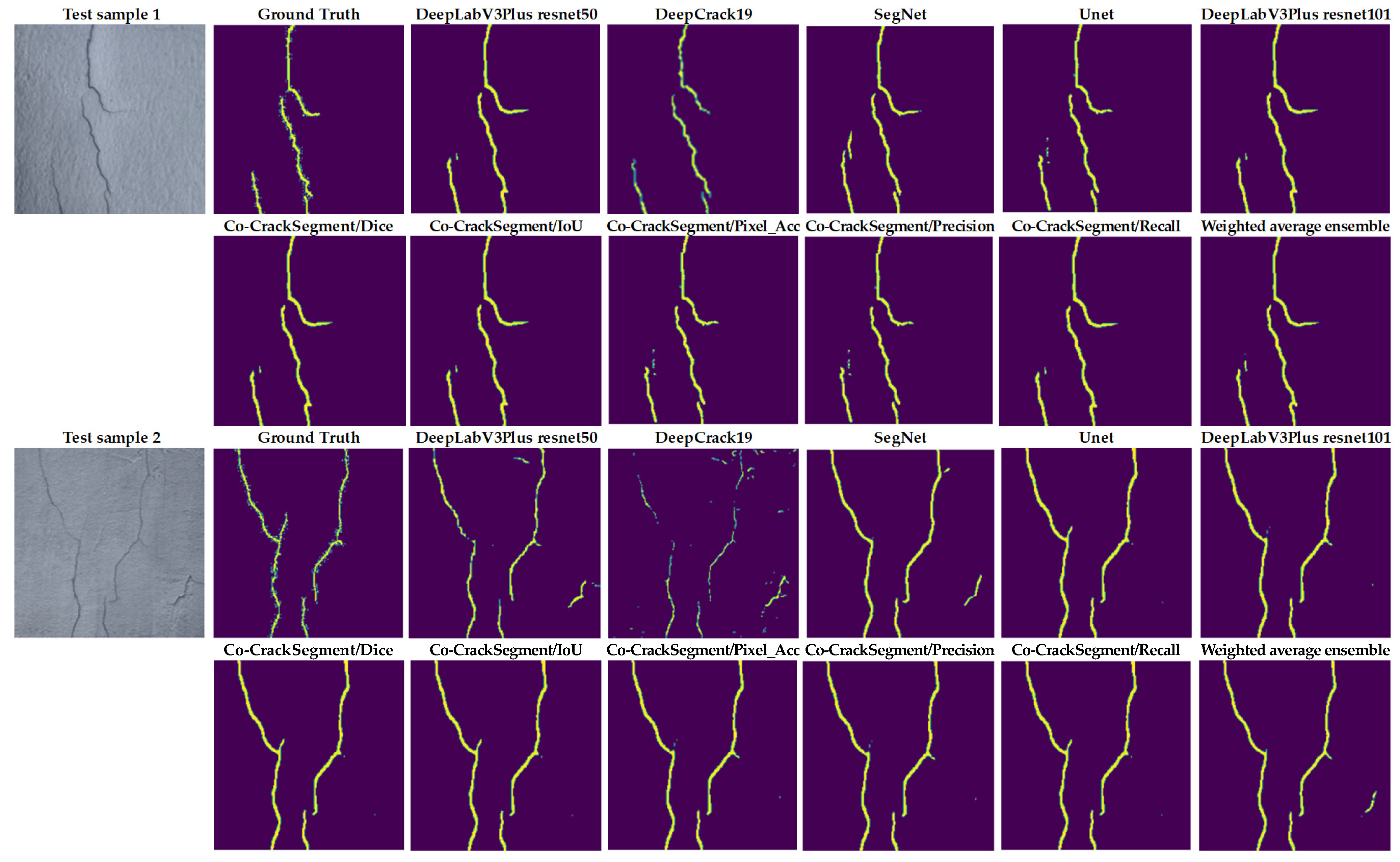
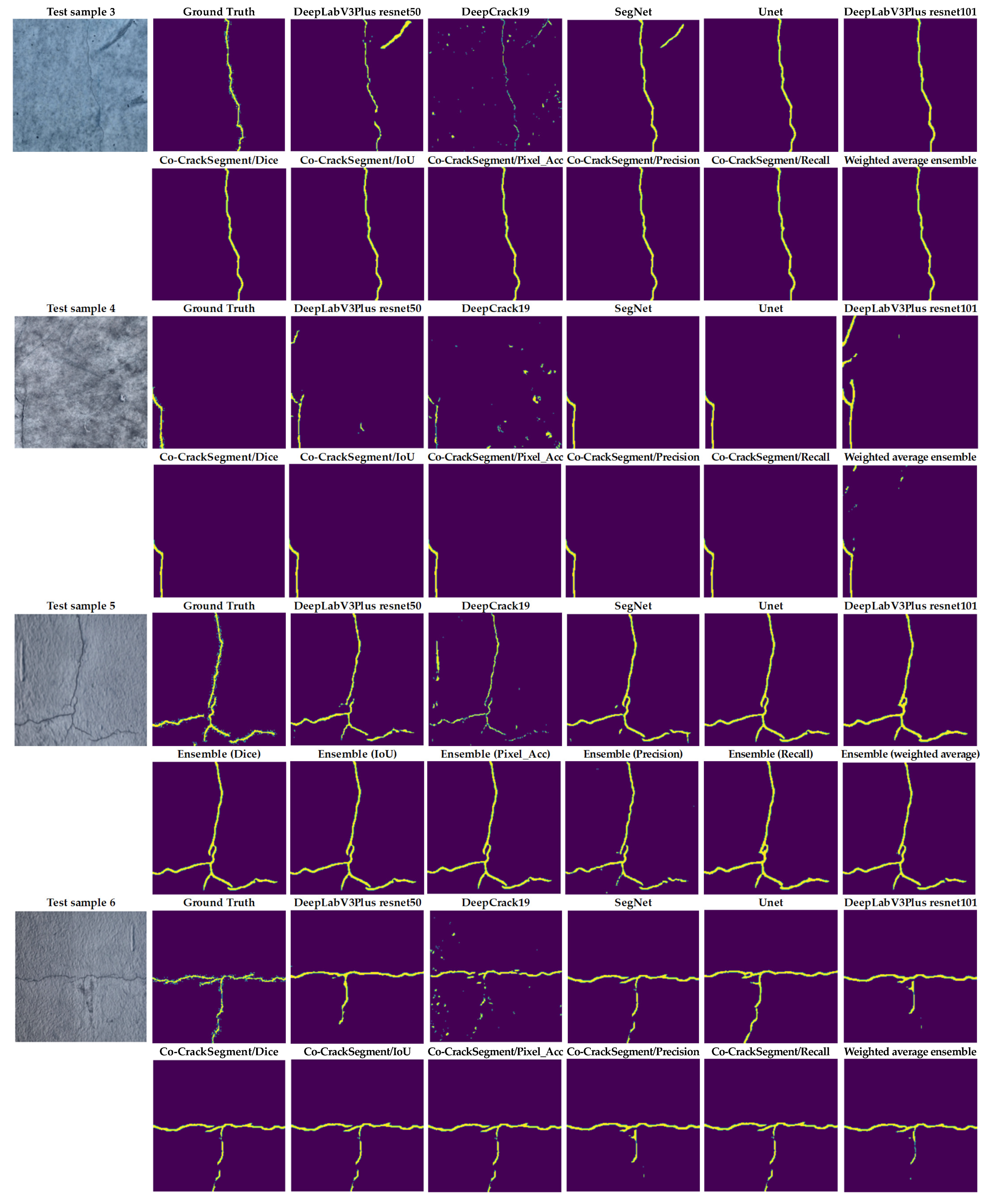

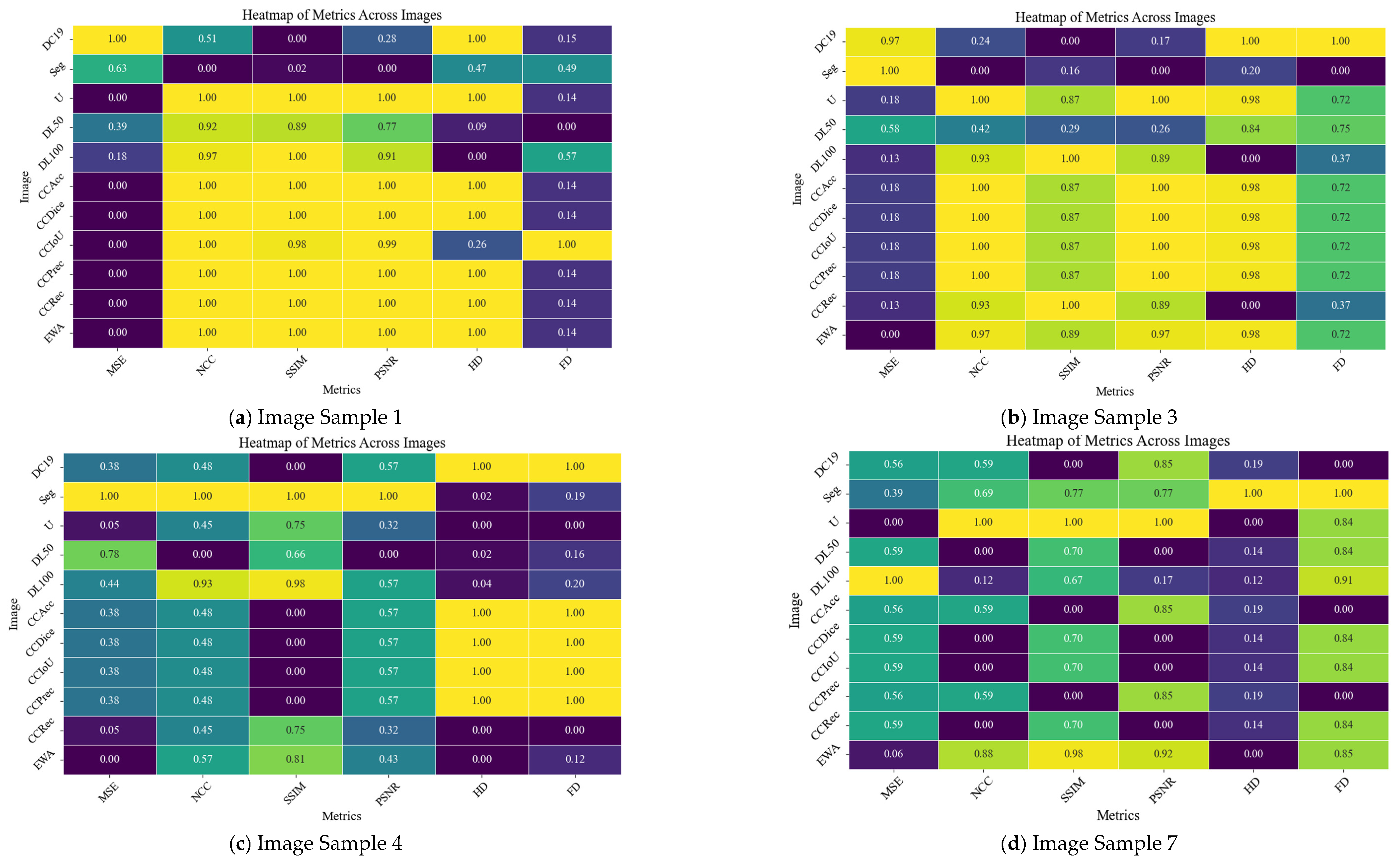
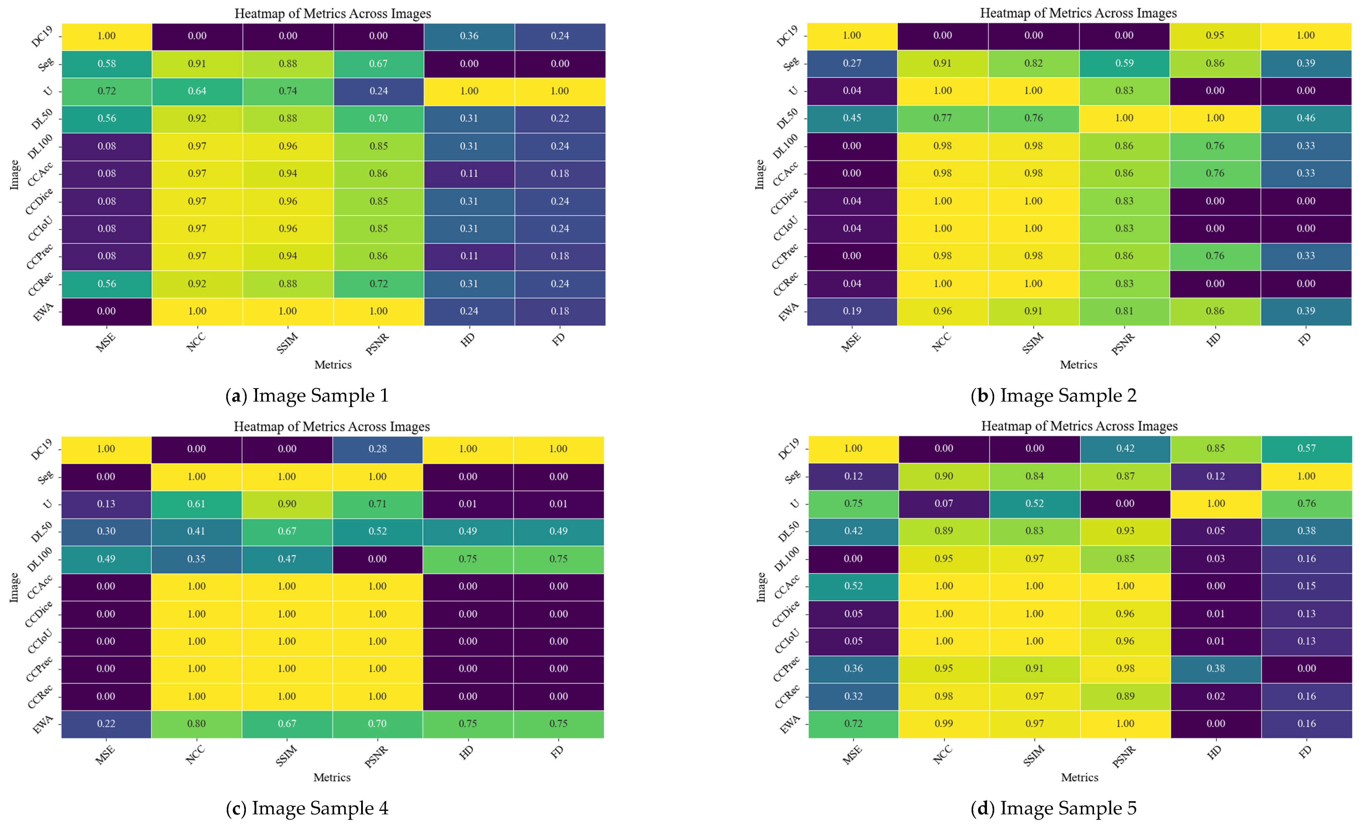
Disclaimer/Publisher’s Note: The statements, opinions and data contained in all publications are solely those of the individual author(s) and contributor(s) and not of MDPI and/or the editor(s). MDPI and/or the editor(s) disclaim responsibility for any injury to people or property resulting from any ideas, methods, instructions or products referred to in the content. |
© 2024 by the authors. Licensee MDPI, Basel, Switzerland. This article is an open access article distributed under the terms and conditions of the Creative Commons Attribution (CC BY) license (https://creativecommons.org/licenses/by/4.0/).