Abstract
This study explores a supply chain product-inventory problem with advance sales under the omni-channel strategies (physical and online sales channels) based on the brand owner’s business model and develops corresponding models that have not been proposed in previous studies. In addition, because the brand owner is a member of the supply chain, and has different handling methods for defective products or products returned by customers in various retail channels, defective products or returned products are included in the supply chain models to comply with actual operating conditions and fill the research gap in the handling of defective/returned products. Regarding the mathematical model’s development, we first clarify the definition of model parameters and relevant data collection, and then establish the production-inventory models with omni-channel strategies and advance sales. The primary objective is to determine the optimal production, delivery, and replenishment decisions of the manufacturer, physical agent, and online e-commerce company in order to maximize the joint total profits of the entire supply chain system. Further, this study takes the supply chain system of mobile game steering wheel products as an example, uses data consistent with the actual situation to demonstrate the optimal solutions of the models, and conducts sensitivity analysis for the proposed model. The findings reveal that increased demand shortens the replenishment cycle and raises order quantity and shipment frequency in the physical channel, similar to the online channel during normal sales. However, during the online pre-order period, higher demand reduces order quantity and cycle length but still increases shipment frequency. Rising ordering or fixed shipping costs lead to higher order quantity and cycle length in both channels, but variable shipping costs in the online channel reduce them. Market price increases boost order quantity and frequency in the online channel, while customer return rates significantly impact inventory decisions.
MSC:
90B05
1. Introduction
Inventory management is a core operational activity for supply chain systems. Effective inventory management is crucial for the healthy functioning of supply chain systems, and related decisions impact the overall financial performance, operational efficiency, and service levels of the entire system [1]. Especially in a brand owner’s operating model, which includes stages such as product design, manufacturing, delivering, replenishment, and sales, the supply chain plays a key role, particularly in managing components and finished goods inventory. Managers must strike a balance between maintaining sufficient inventory to enable the entire supply chain to respond effectively to market changes and minimizing the total cost or maximizing the profit associated with inventory demand. Excess component inventory increases storage and capital costs, while insufficient stock leads to production delays, affecting market responsiveness. Likewise, excess finished goods inventory results in discount pressures, whereas insufficient inventory leads to unmet demand, which harms the brand’s reputation. Therefore, effectively integrating manufacturers and retailers and developing appropriate production-inventory models to jointly determine optimal production, shipping, ordering, and pricing strategies is crucial for supply chain management to minimize total inventory-related cost or maximize overall profit. Goyal [2] pioneered the development of an integrated inventory model for a single manufacturer and a single retailer based on the traditional economic order quantity (EOQ) framework. This seminal study initiated extensive discussions on integrated supply chain inventory models, subsequently leading to the development of various integrated production-inventory models. Banerjee [3] proposed a joint economic lot size (JELS) model, which assumes that the manufacturer produces the entire quantity of products ordered by the retailer and then ships them in bulk to the retailer. Lu [4] extended Banerjee’s model to an integrated inventory model involving a single supplier and multiple buyers. Ha and Kim [5] suggested that goods should be shipped during production to comply with the spirit of just-in-time (JIT). Kelle et al. [6] proposed a production/delivery strategy, where the manufacturer produces quantities that are integer multiple of the quantities received by the retailer each time. Subsequent research, such as that by Ho et al. [7], Lin [8], Wu and Chen [9], Lin and Ho [10], and Lou and Wang [11], continued to explore various aspects of integrated supply chain production-inventory models.
In addition, some practical issues have begun to be incorporated into production-inventory models. For example, Zhao et al. [12] examined an integrated multi-stage supply chain with time-varying demands within a finite planning period. Wu and Zhao [13] considered trade credit policy and explored supply chain inventory models with risk for a single supplier and two retailers. Hariga et al. [14] proposed a model considering carbon tax regulation for a multi-stage cold chain system. Du and Lei [15] discussed competitive and cooperative production-inventory problems in a supply chain that includes a single supplier and multiple retailers. Kogan [16] investigated the impact of wholesale prices with a single price-break point quantity discount on inventory models involving a single supplier and multiple retailers’ competition. Goodarzian et al. [17] developed an integrated supply chain model that integrates production, transportation, ordering, and inventory decisions under various carbon emission regulations. Despite the numerous integrated supply chain models that have been proposed, many primarily focus on physical retail channels and emphasize the production, delivery, and inventory of finished goods, often neglecting raw materials or components. However, the operational framework of the brand owner encompasses omni-channel sales (both physical retail channels and online platform sales channels). Furthermore, the brand owner often faces that the production and sales channels of its products when they come from different countries. Therefore, based on the integrated supply chain production inventory model, this study aims to incorporate the raw materials and finished product inventory of the global supply chain, with the hope that the proposed model can meet the needs of brand owners.
In certain industries, such as electronics retail, services, or seasonal goods, businesses often offer advanced sale services. Examples include advance sales of music C.D.s, books, tickets, and popular travel itineraries. These practices enable firms to extend the sales period and more accurately capture market demand. During the advance sales period, customers can purchase goods at discounted prices, and when the goods arrive, the business can promptly provide them to the customers. Advance sales discounts attract price-sensitive customers who are willing to preorder goods before the official sales season, serving as an effective marketing strategy. Moreover, in competitive markets, many retailers offer advance sales discounts to draw these price-sensitive customers, increase market share, and reduce inventory costs. The sales cycle of goods is becoming increasingly shorter, and many products are sold out after retailers purchase them once. Xie and Shugan [18] proposed that offering discounts to customers during the advance sales period would increase the total profit of the retailer. Moe and Fader [19] utilized demand forecasts from the advance sales period to predict market demand during the on-site sales period. Continuing this line of inquiry, You [20] investigated inventory control issues for stores that exclusively sell goods through advance sales. In his model, customers are allowed to cancel their advance orders, and demand is related to the selling price of the goods. The purpose is to determine the optimal order quantity and selling price that maximizes the retailer’s total profit. You [21] further explored the inventory issue of advance sales, considering scenarios where several pre-sales are offered during the sales period and the demand is dependent on the selling price and waiting time of the customer. You and Wu [22] developed an inventory model that accounted for both advance sales and on-site sales within a finite planning period. Their objective was to determine optimal advance sales prices, on-site selling prices, order quantities, and replenishment frequencies. Tsao [23] discussed two-echelon trade credits and inventory problems involving advance sales and developed an algorithm to determine the optimal replenishment strategy. Chen and Cheng [24] also proposed an inventory model with advance sales that considers the supplier providing incentives for delayed payments to the retailer and the retailer offering advance sales to its customers. Based on the above, this study primarily incorporates advance sales into the production, shipping, and replenishment policies of finished goods and key components based on the current channel sales status of the brand owner.
During the manufacturing process, defective products may arise due to imperfect production systems, old equipment, or human negligence. Therefore, inventory models with imperfect production systems and defective products have been widely proposed [25,26,27,28]. At the earliest, Porteus [29] considered that the quantity of defective products in a production batch is related to the probability of process out of control, and treated the quality level as a decision variable to explore the investment required to improve the production process. Keller and Noori [30] then extended Porteus’s model to include inventory systems with shortages and stochastic demand lead time. Hong and Hayya [31] further generalized Porteus’s approach by incorporating budget constraints and investigating the economic benefits of reducing setup costs and process improvements. Salameh and Jaber [32] introduced the concept of selling defective items at a discounted price after full inspection at the end of a cycle. Subsequently, the inventory model with defective items began to be widely discussed. For instance, Huang [33] developed an integrated inventory model considering defective items from a supply chain perspective. Sana [34] introduced rework concepts to explore inventory models with defective items. Ouyang et al. [35] developed an EOQ model with defective items considering partial delayed payments. Vishkaei et al. [36] investigated optimal replenishment strategies involving inspection and return of defective items. Chen et al. [37] studied the impact of product warranty periods on selling prices. Taleizadeh et al. [38] proposed an inventory model considering defective items and partial backorders. Khalilpourazari and Pasandideh [39] developed a dual-objective Economic Production Quantity (EPQ) model with the stochastic defective rate and allowed shortages. Barzegar and Sajadieh [27] extended Huang’s [33] concept by considering investments to improve defective rates. Priyan and Manivannan [40] explored inventory models with fuzzy deteriorating rates and inspection errors. Nobil et al. [41] addressed procurement-production-inventory problems, considering an imperfect production system under both shortage and non-shortage scenarios. Tiwari et al. [42] developed a stochastic supply chain model in which quality issues and inspection errors impact integration. Zahedi et al. [43] designed a closed loop supply chain system, including forward supply, production, and distribution, as well as reverse inspection, recovery, and disposal. They proposed an integrated objective function to maximize the total profit of the entire supply chain. Because the manufacturer entrusted by the brand owner may produce defective products, in terms of physical channel sales, the defective products produced are not recycled and are directly entrusted to retailers for processing. In the online channel, since the platform allows customers to return goods within a period of time, the returned goods seek to be sold in the secondary market at low prices.
Although numerous integrated supply chain production-inventory models have been proposed, most existing research, such as Goyal [2], Banerjee [3], and Kundu and Chakrabarti [26], primarily focuses on physical retail channels, neglecting the simultaneous management of inventory across both physical and online platforms, particularly in the context of omni-channel strategies. Furthermore, while significant progress has been made in addressing real-world complexities like imperfect production, advance sales, and returns management (e.g., You [20], Tsao [23], Mohanty et al. [28]), these studies have yet to fully capture the interactions between the inventory of key components and finished goods in an omni-channel environment. The term omni-channel refers to a seamless and integrated approach to consumer shopping experiences across multiple channels, both online and in physical retail environments. Among them, the physical store also serves as one of the many touchpoints where customers can interact with a brand. Moreover, many models focus primarily on finished goods and often exclude the critical role of component inventory, which is essential for global supply chains, especially for brand owners operating across multiple countries. This gap becomes more pronounced when factoring in the unique dynamics of online sales, such as advance sales and return policies, which can significantly impact inventory decisions and overall profitability. Therefore, based on the aforementioned relevant literature and the actual situations that the brand owner may face, this study fills an important research gap in the literature by considering the omni-channel strategies included physical and online channels, and exploring a comprehensive production and inventory model with advance sales for the finished goods and key components. To our knowledge, no model for this topic has been proposed before. In the context of the physical retail channel, the primary sales occur through the physical retailer who either sells the goods to customers after manufacturing or serves as one of the many touchpoints where customers can interact with a brand. In the online sales channel, the manufacturer completes production and ships the finished goods to the e-commerce company’s warehouse, which then sells and distributes them through its online shopping platform. Additionally, to strengthen consumers’ willingness to purchase, the brand owner allows its consumers in the online sales channel to apply for returns within an agreed period, and some of the returned items are still usable and sold in the secondary market.
For the proposed model, this study uses mathematical analysis to solve the model and further develops a simple and easy-to-use algorithm to solve the model and verify the results. Furthermore, we employ numerical analysis to illustrate the solution procedure and conduct sensitivity analysis on the major parameters of the model, providing some management implications to enhance the efficiency of brand owners in manufacturing, shipping, sales, and inventory management.
2. Notation and Assumptions
As mentioned above, this study is based on the brand owner’s operating model with the omni-channel strategies included physical retail channels and online sales channels, developing corresponding supply chain production and inventory models. To describe the problem of this study and develop the corresponding supply chain production and inventory model with different retail channels and advance sales, the following notation and assumptions are presented.
2.1. Notations
| i | The subscript symbol, where j = R inducts the physical retailer and j = O inducts the e-commerce company. |
| Demand rate of the physical channel market | |
| Demand rate of the online channel during normal sales period | |
| Demand rate of the online channel during pre-sale period | |
| P | Production rate of the manufacturer |
| S | Setup cost of the manufacturer/production cycle |
| SM | Ordering cost of key components for the manufacturer/production cycle |
| Ordering cost of the facility i/replenishment cycle, where i = R or O | |
| c | Production cost for the manufacturer/unit |
| Purchase cost of key component/unit | |
| Fixed shipping cost of facility i/shipment, where i = R or O | |
| fi | Variable shipping cost of facility i/unit, where i = R or O |
| Holding cost of non-defective items for facility i/unit/unit time, where i = R or O | |
| Holding cost of defective items for facility i/unit/unit time, where i = R or O | |
| hm | Manufacturer’s holding cost of key components/unit/unit time |
| Manufacturer’s holding cost of finished goods for facility i/unit/unit time, where i = R or O | |
| ρ | Product return rate |
| Selling price/unit | |
| s | Selling price in secondary market/unit |
| v | Purchase cost of finished goods for the physical retailer or e-commerce/unit |
| Defective rate of finished goods for the manufacturer | |
| r | Number of key components required per unit of finished goods |
| Length of the pre-order period provided by the e-commerce company | |
| Qi | Order quantity of finished goods for facility i/order, where i = R or O |
| Quantity of finished goods from the manufacturer to facility i/shipment, where i = R or O | |
| Quantity of key components for facility i, where i = R or O | |
| Length of the period required to produce units of finished goods by the manufacturer, where i = R or O | |
| ni | Number of times the manufacturer ships finished goods to facility i within one production cycle, where i = R or O, an integer decision variable |
| Ti | Length of the replenishment cycle of facility i, where i = R or O, a decision variable |
| Length of the manufacturer’s production period within a production cycle for facility i, where i = R or O | |
| Length of the manufacturer’s production cycle for facility i, where i = R or O, a decision variable |
2.2. Assumptions
- This study examines the supply chain system within the brand owner’s operating model, which includes both the physical retail channel and online sales channel, each facing different market demand rates.
- The physical channel comprises a single manufacturer and a single physical retailer. The online sales channel comprises a single manufacturer and a single e-commerce company.
- The proposed supply chain system considers producing a single finished good from a single key component.
- Regardless of the physical retail channel or online sales channel, the manufacturer’s production rate of finished goods is finite and greater than the combined demand rate of the physical retailer and the e-commerce company (such as [13,35,37]). Otherwise, the physical retailer and the e-commerce company will always be out of stock and there will be no inventory issues.
- The e-commerce company offers pre-order services for online sales channels, requiring customers to pay in advance for pre-ordering goods.
- The e-commerce company provides an appreciation period for customers who receive the finished goods. During the appreciation period, the customer can unconditionally request a return and refund if dissatisfied with the finished goods. To facilitate model development, the customer return rate can be estimated from historical data and assumed as a known and fixed value.
- At the end of the sales cycle, all returned finished goods from the online sales channel will be divided into two categories. One category is non-defective products sold in the secondary market at a discounted price, while the other is defective products that are directly discarded.
3. Model Formulation and Solution
Based on the given notation and assumptions, this section will construct a supply chain production-inventory model with omni-channel and advance sales based on the brand owner’s perspective. In the proposed supply chain system, the brand owner entrusts the manufacturer to produce. After receiving the order, the manufacturer purchases key components for finished product production, and then distributes and sells products through the physical retail channel and online sales channel. Regarding the physical retail channel, after manufacturing by the manufacturer, the primary sales occur through the physical retailer who sells the goods to customers. For the online sales channel, the manufacturer completes production and ships the finished goods to the e-commerce company’s warehouse, which then sells and distributes them through its online shopping platform. Additionally, the brand owner allows customers to pre-order goods on the online shopping platform and provides an appreciation period for customers who receive the finished goods. Customers who are dissatisfied during this period can unconditionally request returns and receive refunds. At the end of the sales cycle, the collaborating manufacturers categorize all returned goods from the online platform into two types: non-defective items are sold in the secondary market at a discounted price, while defective items are directly discarded. The procurement of key components, finished product production, transportation, and sales process of the entire supply chain system from the brand owner’s perspective is illustrated in Figure 1.
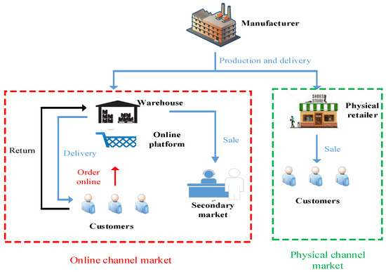
Figure 1.
The entire supply chain system with different retail channels from the brand owner’s perspective.
Next, this study establishes the integrated total profit function of the overall supply chain system including the physical channel retailer, the e-commerce company, and the manufacturer. The details are described as follows:
3.1. Total Profit for the Physical Channel Retailer
For the physical channel retailer, it orders from the manufacturer each time and requires shipments; that is, the quantity of is shipped each replenishment cycle with the length of . Since each batch of finished products will contain defective items with the defect rate λ, a quantity of will be shipped to the physical retailer each time. The inventory level of each replenishment cycle gradually decreases based on market demand, as shown in Figure 2. All the defective items are discarded at the end of each replenishment cycle for the physical retail channel.
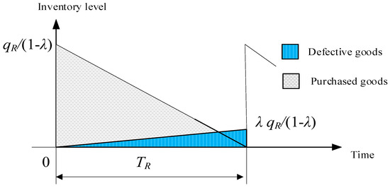
Figure 2.
Inventory level of the physical channel retailer for a replenishment cycle.
Based on the previously defined symbols and assumptions, the total profit function per unit of time for the physical channel retailer can be calculated, including sales revenue, ordering cost, shipping cost, and holding cost. The details are as follows:
- (a)
- Sales Revenue: The sales revenue for the physical retailer per replenishment cycle is equal to .
- (b)
- Ordering Cost: The physical retailer has a fixed ordering cost per replenishment cycle.
- (c)
- Purchasing Cost: For each replenishment cycle, the physical retailer acquires units of non-defective goods, with a unit purchasing price of . Thus, the total purchasing cost for the physical retailer per replenishment cycle is .
- (d)
- Transportation Cost: As the physical retailer requests the manufacturer to deliver the order in shipments, each shipment includes fixed and variable costs, meaning the transportation cost for each replenishment cycle is .
- (e)
- Holding Cost: The holding cost for the physical retailer includes the inventory of non-defective goods and defective products. According to Figure 2, the holding cost for the physical retailer each replenishment cycle can be calculated as:
To summarize the above, and based on the fact that , it can deduct the total profit per unit time for the physical retailer (denoted by ) as:
3.2. Total Profit for the e-Commerce Company
The e-commerce company offers pre-order services with a pre-order period denoted as tp, and provides an appreciation for customers who receive the goods. If customers are not satisfied with the goods in any way, they can unconditionally request a return during the appreciation period (the return rate is ρ). The changes in inventory levels of the e-commerce company in a replenishment cycle are illustrated in Figure 3.
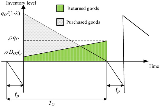
Figure 3.
Inventory level of the e-commerce company for a replenishment cycle.
Similarly, it can calculate the total profit for the e-commerce company, which includes sales revenue, ordering cost, transportation cost, and inventory holding cost, as detailed below.
- (a)
- Sales Revenue: The sales revenue for the e-commerce company for each replenishment cycle with the length of includes both the primary and secondary markets, meaning the sales revenue is equal to .
- (b)
- Ordering Cost: The e-commerce company has a fixed ordering cost for each replenishment cycle.
- (c)
- Purchasing Cost: For each replenishment cycle, the e-commerce company purchases units of non-defective goods, with the unit purchasing price , resulting in a total purchasing cost of .
- (d)
- Transportation Cost: Since the e-commerce company also requests the manufacturer to deliver the order in shipments, each shipment includes fixed and variable costs, resulting in a transportation cost for each replenishment cycle of .
- (e)
- Holding Cost: The holding cost for the e-commerce company includes the inventory of non-defective goods and customer returned products. According to Figure 3, the holding cost for the e-commerce company each replenishment cycle can be calculated as:
To summarize the above, and based on the fact that , it can deduct the total profit per unit time for the e-commerce company (denoted by ) as:
3.3. Total Profit for the Manufacturer
When the manufacturer receives orders from the physical retailer or e-commerce company with the quantity or , the total quantity it will produce and ship is or because there are defective items during the production process. The length of its production period is or . On the other hand, the manufacturer makes key components purchases based on these production quantities, where the purchase quantity is or . Since each unit of finished goods requires r units of key components during production, the inventory level of key components decreases over time at a rate of rP until or is exhausted. Regarding the inventory level of finished goods, because the physical retailer or e-commerce company requires the manufacturer to deliver in batches ( or ), in keeping with the spirit of Just-In-Time (JIT) production, the manufacturer begins shipping items during the production period, delivering the first production up to or to the physical retailer or e-commerce company (the length is or ), and then delivering every fixed interval ( or ) thereafter. Furthermore, based on Assumption 4, the manufacturer stops production after producing the quantity or within the or period, and similarly delivers a fixed quantity or to the physical retailer or e-commerce company every fixed interval ( or ) until all are delivered. The raw material inventory level of the manufacturer fluctuates due to the use of production materials, and the inventory levels of the key components and finished goods for each production cycle are as shown in Figure 4.
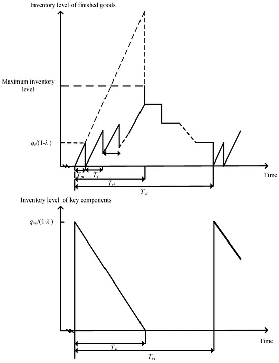
Figure 4.
Inventory levels of manufacturer for each key components and finished goods in a production cycle for different channels (i = R or O).
Based on the aforementioned symbol definitions and assumptions, it can calculate the manufacturer’s total profit per unit of time, which includes sales revenue, setup cost, ordering cost of key components, production cost, purchasing cost of key components, and holding cost, detailed as follows:
- (a)
- Sales Revenue: The sales revenue for the manufacturer in a production cycle comes from both physical and online sales channels, which is equal to v().
- (b)
- Setup Cost: The manufacturer has a fixed setup cost in a production cycle, regardless of the physical and online sales channels; thus, the total setup cost is equal to .
- (c)
- Ordering Cost of Key Components: The manufacturer has a fixed ordering cost in a production cycle, regardless of the physical and online sales channels; thus the total ordering cost of key components is equal to .
- (d)
- Production Cost: The production cost for the manufacturer in a production cycle is .
- (e)
- Purchasing Cost of Key Components: The manufacturer’s purchasing cost of key components for each production cycle is .
- (f)
- Holding Cost: The holding cost for the manufacturer includes two parts: key components and finished goods. Firstly, the inventory level changes for the manufacturer’s key components across different retail channels are as shown in Figure 4. Hence, the total inventory cost of key components is . As for the holding cost of finished goods, since the manufacturer’s cumulative inventory for each production cycle is equal to its cumulative inventory minus the physical retailer’s or the e-commerce company’s cumulative inventory, as shown in Figure 5, the total cumulative inventory of finished goods for the two channels is calculated as:
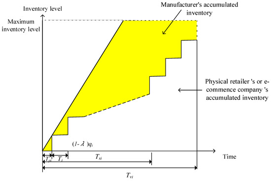 Figure 5. Manufacturer’s cumulative inventory in a production cycle for different channels (i = R or O).
Therefore, the manufacturer’s total holding cost of finished goods is calculated as follows:
Combining the above and based on the fact that , , , and , it can deduct the manufacturer’s total profit per unit time (denoted by ) as:
where i = R and O.
As previously mentioned, it can calculate the integrated total profit per unit time for the entire supply chain (denoted by ) as:
where i = R and O.
Base on the facts that , , and , shown as in (4) can be reduced to , where i = R and O. The main objective is to find the optimal production, delivery, and replenishment strategies from the perspective of supply chain system integration with omin-channel, thereby maximizing the integrated total profit per unit time. First, for given , take the first-order derivatives of with respect to and and let them equal to 0, which gives
and
Since the integrated total profit per unit time, shown in (4), is a complex polynomial function and contains and includes continuous and integer decision variables, it is difficult to solve and prove the concavity of the optimal solution. Instead, we develop the following solution procedure, as shown in Algorithm 1.
| Algorithm 1. The solution procedure of the proposed model with two channels | |
| Step 1: | Start with and , and the initial value of and . |
| Step 2: | Find and (denoted by and ) by solving (5) and (6), and then substitute (, ) into (4) to calculate (denoted by ). |
| Step 3: | Set , and . Then find and (denoted by and ), and substitute (, ) into (4) to calculate (denoted by ). |
| Step 4: | Compare and . (i) If , then go to Step 5. (ii) If , the go back to Step 3. |
| Step 5: | Set , and , and find and (denoted by and ). Then substitute (, ) into (4) to calculate (denoted by ). |
| Step 6: | Compare and . (i) If , then go to Step 7. (ii) If , then back to Step 5. |
| Step 7: | , , , and are the optimal solutions, and the optimal integrated total profit is . |
Although there are some metaheuristic algorithms for solving inventory models, particularly when numerous decision variables are involved, the solution technology we proposed is still an efficient and effective method given the current scale of decision variables.
4. A Numerical Examples and Sensitivity Analysis
4.1. An Empirical Example
The practicality of the proposed model was assessed using a case study involving a brand owner of mobile game steering wheel products in Taiwan. A numerical example of this case was used to verify our analytical results, and sensitivity analysis was used to explore trends in the optimal policies to obtain managerial insights for the footwear manufacturer. Base settings were established for the model by conducting interviews and surveys with relevant staff in this company. The values presented here have been altered to preserve the confidentiality of this commercial information. This research utilized relevant parameter values based on the actual operation of a mobile game steering wheel to verify the inventory model. The descriptions of these parameter values are shown in Table 1.

Table 1.
Parameters of numerical example for the proposed model.
Using the Algorithm 1 above, it was obtained that the manufacturer’s optimal shipping frequency to the physical retailer times and shipping frequency to the e-commerce company times, along with the optimal replenishment cycle length for the physical retailer years, with an order quantity of finished goods 9227.90 units and an order quantity of key components 9513.30 units. The optimal replenishment cycle length for online channels years, with an order quantity of finished goods 7842.82 units and an order quantity of key components 8085.39 units. The optimal integrated total profit for the entire system NT$6.19601 . The solution process is summarized in Table 2. The results of this example can provide the brand owner with a perspective of supply chain system optimization while determining the replenishment quantity of each channel, the manufacturer’s production, and the shipping quantity of key components and finished products.
Table 2.
Solution process of supply chain inventory model base on different channels.
4.2. Sensitivity Analysis
This study conducts sensitivity analysis on the parameters within the model to understand how market variations impact the optimal decisions and total profit of mobile game steering wheel products and key components. We summarize and further interpret the numerical analysis results to provide decision-making references for manufacturers in response to external environmental changes. This study focuses on the sensitivity of the physical channel market demand rate as an example and explores its potential effects on the optimal solution. For convenience, the data are the same as the values used in Section 4.1. Since there are many parameters in the proposed model, the following analysis will be divided into physical retailer’s or e-commerce company’s parameters and manufacturer’s parameters. The results are shown in Table 3 and Table 4.
Table 3.
Sensitivity analysis of physical retailer’s or e-commerce company’s parameters.
Table 4.
Sensitivity analysis of manufacturer’s parameters.
From Table 3, the following observations can be made:
- In the physical channel, when the demand rate increases, the order quantity of finished goods by the physical retailer will increase, but its length of replenishment cycle will shorten. Meanwhile, the number of times the manufacturer ships finished goods to the physical retailer and the quantity of key components ordered by the manufacturer will increase. For the entire supply chain system, the integrated total profit will increase. This empirical result allows the brand owner to effectively monitor demand trends and prepare for frequent restocking in high-demand periods, while optimizing inventory turnover and closely coordinating with suppliers to maintain efficiency and profitability.
- In the online channel, as the demand rate during the normal sales period increases, the order quantity of finished goods and the length of the replenishment cycle for the e-commerce company will increase, along with the frequency of shipments from the manufacturer and the order quantity of key components. Conversely, when the demand rate during the pre-order period increases, the order quantity of finished goods and the replenishment cycle length for the e-commerce company will decrease, while the frequency of shipments from the manufacturer will increase, but the order quantity of key components will decrease. The same as the demand rate of the physical channel, the integrated total profit for the product supply chain system will increase.
- If the ordering cost for the physical retailer or e-commerce company increases, their order quantities of finished goods and length of replenishment cycle will increase. However, while the number of times the manufacturer ships finished goods to the physical retailer or e-commerce company remains unchanged, the manufacturer’s order quantity of key components will increase. Consequently, the integrated total profit for the supply chain system will decrease.
- As the fixed shipping cost for the physical retailer or e-commerce company increases, their order quantities and length of replenishment cycle will increase. Meanwhile, the number of times the manufacturer ships finished goods to the physical retailer or e-commerce company will gradually decrease, and the manufacturer’s order quantity of key components will rise. This will lead to a decrease in the integrated total profit of the supply chain system. These results show that the brand owner should focus on negotiating lower purchase prices and controlling procurement costs, as volume discounts or strategic supplier relationships can mitigate the impact of rising purchase costs on profitability.
- For the physical channel, when the variable shipping cost for the physical retailer increases, the optimal decisions of the physical retailer and the manufacturer remain unaffected, but the integrated total profit will decrease. For the online channel, as the variable shipping cost for the e-commerce company increases, the quantity of finished goods ordered, and the length of the replenishment cycle will decrease. Meanwhile, the number of times the manufacturer ships finished goods to the physical retailer or e-commerce company remains unchanged, but the order quantity of key components will decrease. Consequently, the integrated total profit of the supply chain system will decrease.
- The order quantity of finished goods and length of replenishment cycle will decrease with the increase in the holding cost , , or . However, the number of times the manufacturer ships finished goods to the physical retailer or e-commerce company remains unchanged, and the order quantity of key components decreases. As a result, the integrated total profit for the supply chain system will decrease.
- When the market selling price or secondary market price rises, in the physical channel, the order quantity of finished goods and length of replenishment cycle for the physical retailer, as well as the number of times the manufacturer ships finished goods to the physical retailer and the manufacturer’s order quantity of key component, remain unaffected. However, in the online channel, the order quantity of finished goods and length of replenishment cycle for the e-commerce company will increase, and the number of times the manufacturer ships finished goods to the e-commerce company and the manufacturer’s order quantity of key components will also increase. For the overall supply chain system, total profit will increase whether the market selling or secondary market price rises. These findings allow the brand owner to increase inventory to meet demand when prices in online channels increase, while maintaining operational flexibility and adjusting pricing strategies based on market conditions.
- In the online channel, when the product return rate increases, the order quantity of finished goods and length of replenishment cycle for the e-commerce company will decrease. In addition, the number of times the manufacturer ships finished goods to the e-commerce company remains unchanged, while the manufacturer’s order quantity of key components will decrease. For the overall supply chain system, total profit will decrease. The managerial insight is that the brand owner should implement stricter return policies or improve product quality and customer satisfaction, reduce return frequency and retain profits to mitigate the negative impact of returns.
- When the purchase cost of finished goods increases, the order quantity of finished goods by the physical retailer or the e-commerce company will increase, but the length of the replenishment cycle will shorten. The number of times the manufacturer ships finished goods to the physical retailer or the e-commerce company will increase, and the order quantity of key components will also increase. For the product supply chain system, the integrated total profit will decrease.
From Table 4, the following observations can be made:
- 1
- When the manufacturer’s production rate increases, the order quantities of finished goods by the physical retailer and e-commerce company will decrease, and the corresponding length of the replenishment cycle will shorten. Additionally, the number of times the manufacturer ships finished goods to the physical retailer and the e-commerce company, as well as the manufacturer’s order quantity of key components, will decrease. For the supply chain system, the integrated total profit will increase. From the brand owner’s perspective, optimizing the manufacturer’s production rates can reduce overall inventory levels across the supply chain, improving cash flow and reducing holding costs.
- 2
- As the manufacturer’s setup cost of finished goods or ordering cost of key components increases, the order quantities of finished goods by the physical retailer and e-commerce company will increase, and the corresponding length of the replenishment cycle will lengthen. Moreover, the number of times the manufacturer ships finished goods to the physical retailer and the e-commerce company and the manufacturer’s order quantity of key components will also increase. For the product supply chain system, the integrated total profit will increase.
- 3
- When the manufacturer’s unit production cost of finished goods, unit purchase cost of key components, holding cost or increases, the frequency of shipments to the physical retailer or e-commerce company will gradually decrease. In addition, although the length of the replenishment cycle for the physical retailer or e-commerce company will lengthen as the frequency of shipments decreases, both the order quantity of finished goods and the manufacturer’s order quantity of key components will decrease. For the supply chain system, the integrated total profit will decrease.
- 4
- When the holding cost of key components increases, the order quantity of finished goods and the length of replenishment cycle for the physical retailer or e-commerce company will decrease; meanwhile, the manufacturer’s shipment frequency and the manufacturer’s order quantity of key components will gradually decrease. For the supply chain system, the integrated total profit will increase.
- 5
- When the defective rate increases, the order quantity of finished goods and the length of the replenishment cycle for the physical retailer or e-commerce company will decrease; the manufacturer’s shipment frequency will remain unchanged, but its order quantity of key components ordered will decrease. For the supply chain system, the integrated total profit will increase. This implies that investing in quality control measures and supplier management can help maintain optimal inventory levels and shipping schedules for the brand owner.
- 6
- When the value of parameter r increases, the order quantity of finished goods and the length of the replenishment cycle for the physical retailer or e-commerce company will decrease; meanwhile, the manufacturer’s shipment frequency will gradually decrease, but its order quantity of key components will increase. For the supply chain system, the integrated total profit will increase.
The aforementioned sensitivity analysis results offer the brand owner valuable insights for making optimal decisions in response to changing conditions. Additionally, the proposed model improves upon existing production-inventory frameworks by integrating omni-channel strategies and tackling the complexities associated with defective and returned products, thus providing a more comprehensive approach compared to previous studies. That is, our model builds upon these foundations, offering a more nuanced framework that provides practical insights for the brand owner and demonstrates its superiority in addressing contemporary challenges in supply chain management.
5. Conclusions
This study primarily developed a production-inventory model incorporating omni-channel strategies and advance sales from the perspective of brand owners. Further, it incorporated handling strategies for defective and returned products, reflecting real-world complexities and providing practical insights for brand owners. This research not only established a model for the brand’s finished products and key components based on the optimal delivery times, replenishment cycles, and order quantities of the finished products and key components in different retail channels, but also developed a simple algorithm to solve the proposed model. Furthermore, numerical examples that are relatively consistent with practice are used to solve and verify the model, followed by a sensitivity analysis is performed on the model parameters to provide a reference for comparison with traditional empirical decision-making, and to adjust the optimal decision promptly.
Compared with previous studies, the proposed model enhances existing production-inventory frameworks by incorporating omni-channel strategies and addressing the complexities of defective and returned products. For instance, prior research by You [20] focused on the ordering and pricing of service products in an advance sales system, assuming price-dependent demand, while this study captures the mutual influence of prices on demand across physical and online channels. Similarly, Tsao [23] explored optimal ordering and discounting policies under advance sales, highlighting the importance of pricing strategies; the presented model integrates these concepts while also accounting for defective and returned products. Kundu and Chakrabarti [26] developed a multi-stage supply chain inventory model that addresses imperfections in the production process, which aligns with the complexities considered in this study. Meanwhile, Mohanty et al. [28] examined vendor–buyer interactions in production-inventory systems under trade credit, but did not fully account for the impact of omni-channel strategies. In summary, the current model builds these earlier works by offering a more comprehensive framework that provides practical insights for the brand owner and demonstrating its superiority in addressing contemporary challenges in supply chain management.
Based on the numerical analysis and sensitivity analysis results, in addition to some common sense knowledge, such as demand growth contributing to the total profit and cost increase reducing the total profit for the supply chain, the following meaningful insights can be obtained: (1) In the physical channel, higher demand leads to increased order quantity and shipment frequency, with a shorter replenishment cycle. This result is the same as that of the online channel during the normal sales period. However, in the online channel during the pre-order period, higher demand reduces order quantity and replenishment cycle but still increases shipment frequencies. Strengthening supplier relationships is crucial to managing increased demand effectively and ensuring a steady supply of components. (2) For physical retailers or e-commerce companies, when ordering cost or fixed shipping cost increases, both the order quantity and replenishment cycle length rise. In the physical channel, rising variable shipping costs do not change the retailer’s or manufacturer’s decisions. In contrast, in the online channel, these costs reduce order quantities and cycle length. (3) When the market or secondary market price rises, physical channel operations remain unchanged, but in the online channel, both the order quantity and replenishment cycle increase. This leads to more frequent shipments and higher order quantities of key components, resulting in an overall increase in total supply chain profit. (4) The customer return rate is an important factor affecting production inventory decisions. The relaxed return policy of online e-commerce company will shorten its order quantity of finished goods and key components, as well as the replenishment cycle.
This study has several research limitations and the following future directions can be considered. First, to facilitate model solutions, this study considers the selling prices of physical and online channels as given parameters, which implies the decision-making of these two channels is independent. However, in actual scenarios, the demand for physical and online channels may affect prices individually and mutually. Therefore, in future research, a demand function influenced by the price of its channel and the prices of other channels could be considered, with pricing decisions also included in the model. Second, the existing model only considers a single finished good and a single key component. If it can be extended to multiple finished goods or incorporate multiple components, the applicability of the proposed model would be expanded. Finally, the current focus on net-zero carbon emissions has attracted attention from governments, relevant organizations, and customers. For the brand owner, incorporating carbon footprint considerations and integrating carbon taxes, carbon fees, or carbon emission reduction policies into the model is an interesting and necessary research direction.
Author Contributions
J.P. and W.-J.C. have equivalent contributions as the first author. J.P.: Conceptualization, methodology, formal analysis, writing—original draft preparation; W.-J.C.: Conceptualization, methodology, formal analysis, writing—original draft preparation; C.-J.L.: Conceptualization, methodology, supervision, writing—original draft preparation; K.-S.W.: Methodology, supervision, writing—original draft preparation; C.-T.Y.: Writing—original draft preparation. All authors have read and agreed to the published version of the manuscript.
Funding
The authors received no financial support for the research, authorship, and publication of this article.
Data Availability Statement
The datasets used and/or analyzed during the current study are available from the corresponding author on reasonable request at 122300@mail.tku.edu.tw.
Conflicts of Interest
The authors declare that they have no competing interests.
References
- Nemati, Y.; Alavidoost, M.H. A fuzzy bi-objective MILP approach to integrate sales, production, distribution and procurement planning in a FMCG supply chain. Soft Comput. 2019, 23, 4871–4890. [Google Scholar] [CrossRef]
- Goyal, S.K. An integrated inventory model for a single supplier-single customer problem. Int. J. Prod. Res. 1976, 15, 107–111. [Google Scholar] [CrossRef]
- Banerjee, A. A joint economic-lot-size model for purchaser and vendor. Decis. Sci. 1986, 17, 292–311. [Google Scholar] [CrossRef]
- Lu, L. A one-vendor multi-buyer integrated inventory model. Eur. J. Oper. Res. 1995, 81, 312–323. [Google Scholar] [CrossRef]
- Ha, D.; Kim, S.L. Implementation of JIT purchasing: An integrated approach. Prod. Plan. Control 1997, 8, 152–157. [Google Scholar] [CrossRef]
- Kelle, P.; Al-khateeb, F.; Miller, P.A. Partnership and negotiation support by joint optimal ordering/setup policies for JIT. Int. J. Prod. Econ. 2003, 81–82, 431–441. [Google Scholar] [CrossRef]
- Ho, C.H.; Ouyang, L.Y.; Su, C.H. Optimal pricing, shipment and payment policy for an integrated supplier-buyer inventory model with two-part trade credit. Eur. J. Oper. Res. 2008, 187, 496–510. [Google Scholar] [CrossRef]
- Lin, Y.J. An integrated vendor-buyer inventory model with backorder price discount and effective investment to reduce ordering cost. Comput. Ind. Eng. 2009, 56, 1597–1606. [Google Scholar] [CrossRef]
- Wu, O.Q.; Chen, H. Optimal control and equilibrium behavior of production-inventory systems. Manag. Sci. 2010, 56, 1362–1379. [Google Scholar] [CrossRef]
- Lin, Y.J.; Ho, C.H. Integrated inventory model with quantity discount and price-sensitive demand. TOP 2011, 19, 177–188. [Google Scholar] [CrossRef]
- Lou, K.R.; Wang, W.C. A comprehensive extension of an integrated inventory model with ordering cost reduction and permissible delay in payments. Appl. Math. Model. 2013, 37, 4709–4716. [Google Scholar] [CrossRef]
- Zhao, S.T.; Wu, K.; Yuan, X.M. Optimal production-inventory policy for an integrated multi-stage supply chain with time-varying demand. Eur. J. Oper. Res. 2016, 255, 364–379. [Google Scholar] [CrossRef]
- Wu, C.; Zhao, Q. Two retailer–supplier supply chain models with default risk under trade credit policy. SpringerPlus 2016, 5, 1728. [Google Scholar] [CrossRef] [PubMed]
- Hariga, M.; As’ad, R.; Shamayleh, A. Integrated economic and environmental models for a multi stage cold supply chain under carbon tax regulation. J. Clean. Prod. 2017, 166, 1357–1371. [Google Scholar] [CrossRef]
- Du, J.; Lei, Q. Competition and coordination in single-supplier multiple-retailer supply chain. In Recent Developments in Data Science and Business Analytics; Springer: Cham, Switzerland, 2018; pp. 45–53. [Google Scholar]
- Kogan, K. Discounting revisited: Evolutionary perspectives on competition and coordination in a supply chain with multiple retailers. Cent. Eur. J. Oper. Res. 2019, 27, 69–92. [Google Scholar] [CrossRef]
- Goodarzian, F.; Kumar, V.; Abraham, A. Hybrid meta-heuristic algorithms for a supply chain network considering different carbon emission regulations using big data characteristics. Soft Comput. 2021, 25, 7527–7557. [Google Scholar] [CrossRef]
- Xie, J.; Shugan, S.M. Electronic tickets, smart cards, and online prepayments when and how to advance sell. Manag. Sci. 2001, 20, 219–243. [Google Scholar] [CrossRef]
- Moe, W.W.; Fader, P.S. Using advance purchase orders to forecast new product sales. Mark. Sci. 2002, 21, 347–364. [Google Scholar] [CrossRef]
- You, P.S. Ordering and pricing of service products in an advance sales system with price-dependent demand. Eur. J. Oper. Res. 2006, 170, 51–71. [Google Scholar] [CrossRef]
- You, P.S. Optimal pricing for an advance sales system with price and waiting time dependent demands. J. Oper. Res. Soc. Jpn. 2007, 50, 151–161. [Google Scholar] [CrossRef]
- You, P.S.; Wu, M.T. Optimal Ordering and pricing policy for an inventory system with order cancellations. OR Spectr. 2007, 29, 661–679. [Google Scholar] [CrossRef]
- Tsao, Y.C. Retailer’s optimal ordering and discounting policies under advance sales discount and trade credits. Comput. Ind. Eng. 2009, 56, 208–215. [Google Scholar] [CrossRef]
- Chen, M.L.; Cheng, M.C. Optimal order quantity under advance sales and permissible delays in payments. Afr. J. Bus. Manag. 2011, 17, 7325–7334. [Google Scholar]
- Ullah, M.; Kang, C.W. Effect of rework, rejects and inspection on lot size with work-in-process inventory. Int. J. Prod. Res. 2014, 52, 2448–2460. [Google Scholar] [CrossRef]
- Kundu, S.; Chakrabarti, T. An integrated multi-stage supply chain inventory model with imperfect production process. Int. J. Ind. Eng. Comput. 2015, 6, 568–580. [Google Scholar] [CrossRef]
- Barzegar Astanjin, M.; Sajadieh, M.S. Integrated production-inventory model with price-dependent demand, imperfect quality, and investment in quality and inspection. AUT J. Model. Simul. 2017, 49, 43–56. [Google Scholar]
- Mohanty, D.J.; Kumar, R.S.; Goswami, A. Vendor-buyer integrated production-inventory system for imperfect quality item under trade credit finance and variable setup cost. RAIRO-Oper. Res. 2018, 52, 1277–1293. [Google Scholar] [CrossRef]
- Porteus, E.L. Optimal lot sizing, process quality improvement and setup cost reduction. Oper. Res. 1986, 34, 137–144. [Google Scholar] [CrossRef]
- Keller, G.; Noori, H. Impact of investing in quality improvement on the lot size model. Omega 1988, 16, 595–601. [Google Scholar] [CrossRef]
- Hong, J.D.; Hayya, J.C. Joint investment in quality improvement and setup reduction. Comput. Oper. Res. 1995, 22, 567–574. [Google Scholar] [CrossRef]
- Salameh, M.K.; Jaber, M.Y. Economic production quantity model for items with imperfect quality. Int. J. Prod. Econ. 2000, 64, 59–64. [Google Scholar] [CrossRef]
- Huang, C.K. An optimal policy for a single-vendor single-buyer integrated production– inventory problem with process unreliability consideration. Int. J. Prod. Econ. 2004, 91, 91–98. [Google Scholar] [CrossRef]
- Sana, S.S. A production–inventory model in an imperfect production process. Eur. J. Oper. Res. 2010, 200, 451–464. [Google Scholar] [CrossRef]
- Ouyang, L.Y.; Chang, C.T.; Shum, P. The EOQ with defective items and partially permissible delay in payments linked to order quantity derived algebraically. Cent. Eur. J. Oper. Res. 2012, 20, 141–160. [Google Scholar] [CrossRef]
- Vishkaei, B.M.; Niaki, S.T.A.; Farhangi, M.; Rashti, M.E.M. Optimal lot sizing in screening processes with returnable defective items. J. Ind. Eng. Int. 2014, 10, 70. [Google Scholar] [CrossRef]
- Chen, C.K.; Lo, C.C.; Weng, T.C. Optimal production run length and warranty period for an imperfect production system under selling price dependent on warranty period. Eur. J. Oper. Res. 2016, 259, 401–412. [Google Scholar] [CrossRef]
- Taleizadeh, A.A.; Khanbaglo, M.P.S.; Cárdenas-Barrón, L.E. An EOQ inventory model with partial backordering and reparation of imperfect products. Int. J. Prod. Econ. 2016, 182, 418–434. [Google Scholar] [CrossRef]
- Khalilpourazari, S.; Pasandideh, S.H.R. Bi-objective optimization of multi-product EPQ model with backorders, rework process and random defective rate. In Proceedings of the 2016 12th International Conference on Industrial Engineering (ICIE), Tehran, Iran, 25–26 January 2016; IEEE: New York, NY, USA, 2016; pp. 36–40. [Google Scholar]
- Priyan, S.; Manivannan, P. Optimal inventory modeling of supply chain system involving quality inspection errors and fuzzy defective rate. Opsearch 2017, 54, 21–43. [Google Scholar] [CrossRef]
- Nobil, A.H.; Cárdenas–Barrón, L.E.; Nobil, E. Optimal and simple algorithms to solve integrated procurement-praaoduction-inventory problem without/with shortage. RAIRO-Oper. Res. 2018, 52, 755–778. [Google Scholar] [CrossRef]
- Tiwari, S.; Kazemi, N.; Modak, N.M.; Cárdenas-Barrón, L.E.; Sarkar, S. The effect of human errors on an integrated stochastic supply chain model with setup cost reduction and backorder price discount. Int. J. Prod. Econ. 2020, 226, 107643. [Google Scholar] [CrossRef]
- Zahedi, A.; Salehi-Amiri, A.; Hajiaghaei-Keshteli, M.; Diabat, A. Designing a closed-loop supply chain network considering multi-task sales agencies and multi-mode transportation. Soft Comput. 2021, 25, 6203–6235. [Google Scholar] [CrossRef]


Disclaimer/Publisher’s Note: The statements, opinions and data contained in all publications are solely those of the individual author(s) and contributor(s) and not of MDPI and/or the editor(s). MDPI and/or the editor(s) disclaim responsibility for any injury to people or property resulting from any ideas, methods, instructions or products referred to in the content. |
© 2024 by the authors. Licensee MDPI, Basel, Switzerland. This article is an open access article distributed under the terms and conditions of the Creative Commons Attribution (CC BY) license (https://creativecommons.org/licenses/by/4.0/).