Abstract
The multiple regression model statistical technique is employed to analyze the relationship between the dependent variable and several independent variables. The multicollinearity problem is one of the issues affecting the multiple regression model, occurring in regard to the relationship among independent variables. The ordinal least square is the standard method to evaluate parameters in the regression model, but the multicollinearity problem affects the unstable estimator. Liu regression is proposed to approximate the Liu estimators based on the Liu parameter, to overcome multicollinearity. In this paper, we propose a modified Liu parameter to estimate the biasing parameter in scaling options, comparing the ordinal least square estimator with two modified Liu parameters and six standard Liu parameters. The performance of the modified Liu parameter is considered, generating independent variables from the multivariate normal distribution in the Toeplitz correlation pattern as the multicollinearity data, where the dependent variable is obtained from the independent variable multiplied by a coefficient of regression and the error from the normal distribution. The mean absolute percentage error is computed as an evaluation criterion of the estimation. For application, a real Hepatitis C patients dataset was used, in order to investigate the benefit of the modified Liu parameter. Through simulation and real dataset analysis, the results indicate that the modified Liu parameter outperformed the other Liu parameters and the ordinal least square estimator. It can be recommended to the user for estimating parameters via the modified Liu parameter when the independent variable exhibits the multicollinearity problem.
MSC:
62J02; 62J05; 62J07; 62J20; 62P25
1. Introduction
Regression analysis is a potent statistical tool that reveals the connections between one or more independent variables and a dependent variable. Essential in data analysis and predictive modeling, it finds broad application across fields such as economics, finance, healthcare, and social sciences. However, regression models must meet certain assumptions to provide reliable and valid results. These assumptions form the foundation of regression analysis and guide researchers in interpreting results accurately. One problematic assumption to avoid is the linear relationship among independent variables called multicollinearity, which occurs when two or more independent variables are correlated, increasing the standard error of the coefficients. This escalation in standard errors can render the coefficients of certain independent variables statistically insignificant despite their potential significance. In essence, multicollinearity distorts the interpretation of variables by inflating their standard errors [1]. Shrestha [2] discussed the primary techniques for investigating multicollinearity using questionnaires for survey data to support customer satisfaction.
The Toeplitz correlation structure is a specific type of correlation pattern frequently appearing in real-world datasets such as financial time series data, spatial models, climate data, correlation in DNA sequences, and time-dependent traffic patterns. The properties of Toeplitz covariance matrices have been extensively applied across various fields, with early examples found in psychometric and medical research [3]. Furthermore, the Toeplitz correlation structure is a part of multicollinearity, often arising in datasets with variables exhibiting inherent relationships. Qi et al. [4] utilized a multiple-Toeplitz matrix reconstruction method with quadratic spatial smoothing to enhance direction-of-arrival estimation performance for coherent signals under low signal-to-noise ratio conditions.
Traditional regression techniques often struggle to handle multicollinearity effectively, leading to biased results and unreliable predictions. Researchers have developed various methods to mitigate these challenges, including Liu regression. Liu regression is a technique designed to address multicollinearity in regression analysis. It combines the principles of ridge regression with orthogonalization to effectively mitigate the effects of multicollinearity. Dawoud et al. [5] devised a novel modified Liu estimator to employ multicollinearity in a regression model with a single parameter, incorporating two biasing parameters, with at least one designed to mitigate this issue. Jahufer [6], on the other hand, employed the Liu estimator to alleviate the impact of multicollinearity and the influence of specific observations, devising approximate deletion formulas for identifying influential points.
In predictive analytics, the search for accurate models that can efficiently handle complex datasets while offering robust predictions is perpetual. Among the array of methodologies, the Liu regression model enables better control over the trade-off between bias and variance, leading to more stable and reliable parameter estimates. The flexibility of the Liu estimator makes it a valuable tool in the modern statistician’s toolkit, particularly in fields where predictive accuracy is critical. Karlsson et al. [7] introduced a Liu estimator tailored for the beta regression model with a fixed dispersion parameter, applicable in various practical scenarios where the correlation level among the regressors varies.
Liu regression [8] involves selecting a Liu estimator to balance the bias–variance trade-off. The optimal value of the Liu estimator is typically chosen through techniques such as cross-validation. The Liu estimator, named after its developer, is essential in managing multicollinearity. It is particularly associated with methodologies like ridge regression with orthogonalization, often abbreviated as Liu regression. Liu [9] enhanced the Liu estimator within the linear regression model by considering the biasing parameter under the prediction sum-of-squares criterion. Yang and Xu [10] proposed an alternative stochastic restricted Liu estimator for the parameter vector in a linear regression model, incorporating additional stochastic linear restrictions. Hubert and Wijekoon [11] investigated a novel Liu-type biased estimator, termed the stochastic restricted Liu estimator, and examined its efficiency.
The improvement of the Liu estimator transformed the multiple regression model to canonical form [12] to select a biasing parameter called the Liu parameter. The appropriate Liu parameters were developed to obtain the minimum mean square error in the estimation. Liu [8,9] applied the iterative method to estimate the Liu parameter as the minimum mean squares error in the Liu estimator. Özkale and Kaçiranlar [13] proposed a new restricted Liu parameter by computing the predicted residual error sum of squares to determine the biasing parameter. Dawoud et al. [5] proposed a new Liu estimator using the known mean squares error criterion to handle the multicollinearity problem. Suhail et al. [14] developed a new method of biasing parameters to mitigate the multicollinearity data. Lukman et al. [15] introduced a modified Liu estimator to address multicollinearity issues within the linear regression model.
In this paper, we propose two competing Liu parameters, following mean squares error and R-squared approaches, to estimate the Liu estimator via a multiple regression model with the multicollinearity problem. We measure this performance using the minimum average mean absolute percentage errors for the simulation and real dataset. We also consider the scale option of independent variables including the center, correlation form, and standardization.
This paper is structured as follows: Section 2 presents the multiple regression estimators and discusses the Liu estimator through the reparameterization of Liu regression in canonical form, then in comparison with the OLS estimator. Section 3 describes generation of the independent and dependent variables to evaluate the performance estimators. Section 4 applies a real dataset to validate the simulation results. Section 5 discusses the findings, followed by the conclusion in Section 6.
2. Liu Regression
The multiple regression model is expressed in matrix form as follows:
where is the a column vector of the dependent variable, is the independent variable matrix, is the multiple regression parameter vectors, and is the error vector. The following assumptions of error are made: , , and The efficient parameters () in (1) are commonly estimated to obtain the ordinary least squares (OLS) estimator in (2), as follows:
The estimation error of is evaluated by computing:
The bias, variance (Var), and mean squares error (MSE) of the OLS estimator are computed from (3) as follows:
Hoel and Kennard [16] proposed ridge regression, a powerful technique for handling multicollinearity in linear regression models. Ridge regression addresses the issue by adding a penalty term to the ordinary least squares (OLS) estimation process, shrinking the coefficients towards zero. This regularization helps reduce model complexity and improve prediction accuracy. The ridge regression estimator is expressed as follows:
where is the regularization parameter controlling the shrinkage amount.
From the above computation, the OLS estimator presents the unbiased estimator, which reduces the performance in estimating parameters in relation to the multicollinearity of independent variables. The diagonal matrix causes multicollinearity and inflation, increasing the estimated variance and mean squares error. To overcome this problem, Liu [8] proposed the Liu estimator, which performs better than the OLS estimator [13,17]. The Liu estimator is written based on the OLS as follows:
where is the Liu parameter in terms of the biasing parameter and is the identity matrix. The OLS form (2) and Liu estimators from (5) are related to the independent variables affected by the multicollinearity problem because they depend on the OLS estimator.
The estimation error of is evaluated as the OLS estimator by comparing the Liu estimator and the parameter of the multiple regression model:
The bias [18], variance (Var), and mean square error (MSE) of the Liu estimator from (6) are proposed in the following:
The Liu estimator is shown as the bias estimator, and its variance is greater than that of the OLS estimator when lies between zero and one. Subsequently, Liu [9] developed the shrinkage factor [19] to create the Liu parameter that may lie outside the range between zero and one. In the following subsection, the multiple regression model is transformed into a canonical form to estimate the OLS and Liu estimators.
2.1. The Reparameterization of Liu Regression
The reparameterization of Liu regression transforms a multiple regression model into a canonical form, offering valuable insights into variable relationships and enhancing predictive accuracy [19]. The optimal Liu parameter is determined by minimizing the mean squares error. Akdeniz and Kacįranlar [20] introduced a new biased estimator and assessed its performance against a restricted least squares estimator regarding mean squares error. The comparison of the Liu estimator’s performance in canonical form is expressed as follows:
where , , , and is a diagonal matrix such that . The OLS estimator in canonical form can be defined as follows:
Similarly, the Liu estimator [21] can be written as follows:
The bias, variance (Var), and mean square error (MSE) of the reparameterization of the OLS estimator from (8) are expressed as follows:
The bias, variance (Var), and mean square error (MSE) of the reparameterization of the Liu estimator from (9) are proposed in the following:
Furthermore, the bias, variance, and mean squares error are given by Equations (13), (14), and (15), respectively:
The OLS and Liu estimators in canonical form were compared by considering the variance and MSE.
Given the and , the is the better estimator than , that is , if and only if
Recall that:
and
Then:
It can be observed that when . It can be concluded that and the Liu estimator outperforms the OLS estimator.
2.2. Liu Parameter
As per the above subsection, we compared the two estimators. The reparameterization of Liu regression provides the performance estimator. However, the existing Liu estimator is to select the appropriate Liu parameter that was started by Liu [8] and developed into another model by Suhail et al. [14], Lukman et al. [15], Abdelwahab et al. [22], and Babar et al. [23]. The optimal Liu parameter is one reason to make the minimum of mean squares error (MSE) that is excessed to affect the estimation of the Liu estimator of collinearity on independent variables. However, tracing a diagonal matrix of transformation is useful for calculating the optimal Liu parameter. In this article, we suggest a version of the original Liu parameter, which was proposed by Liu [8], which is defined according to the optimum (opt), the minimum MSE (mm), and Cl criterion (cl), respectively, as follows:
From (15), the mean squares error (MSE) of the estimator is given by:
Now, we need to differentiate the MSE concerning . This involves differentiating both the variance and bias terms as follows:
From (17), this equation and solving for yield the optimal , then:
After solving, the is given by:
where as the estimated standard deviation of the error term in the regression model and as the estimated coefficients in the canonical form of the Liu regression model.
From (17), the minimum MSE is to substitute and for their unbiased estimator, and the derivative of the MSE with respect to is set to zero:
Minimizing the MSE leads to the following expression for :
The Liu parameter from the CL criterion is used to find the optimal biasing parameter that minimizes the CL criterion, which balances the trade-off between fitting the data well and keeping the model’s complexity under control. The following formula gives the CL criterion:
where is the residual sum of squares, , and is the estimated variance of the errors.
To find the optimal , we need to take the derivative of the CL criterion with respect to and set it to zero: .
After calculating the derivative and rearranging as and , we obtain the following equation:
Furthermore, Liu [9] improved the Liu parameter in multiple linear regression under the approximation of the predicted residual error sum of squares criterion via the improved Liu estimator (ILE) as follows:
where
and
Özkale and Kaçiranlar [13] introduced a new two-parameter approach by incorporating the contraction estimator, encompassing well-known methods such as restricted least squares, restricted ridge, restricted contraction estimators, and a novel modified, restricted Liu estimator (RLE), which can be written as follows:
where represents the diagonal elements from the matrix ;
represents the diagonal elements from the matrix ;
represents the diagonal elements from the Liu hat matrix from (5) with cross-validation implemented to evaluate MSE for [24],
and is the ith residual at a specific value of .
- Mallows [25] discussed the interpretation of Cp plots by using the display as a basis for formally selecting a subset-regression model and extending to estimate the Liu estimator. The Liu parameter is defined as follows:where
In this paper, we modify the Liu parameter from Mallows [25] to introduce the mean squares error, which is obtained via the mean sum of squares residual (SSR) as follows:
Furthermore, the correlation coefficient, often denoted as R-squared (), is a critical metric in regression analysis. It quantifies the proportion of the variance in the dependent variable that can be predicted from the independent variables. From the significance of R-squared, we propose the new Liu parameter by computing the correlation coefficient as in the range between zero and one, which is rewritten as follows:
where represents the diagonal elements from and represents the diagonal elements from
Scaling options are utilized to standardize the independent variables and assess their performance via the Liu estimator. The initial method, introduced by Liu [8], is the centered option, standardizing independent variables to have zero mean and unit variance. The scaled option further standardizes independent variables. Lastly, the SC option scales independent variables in correlation form, a concept explored by Belsley [26].
3. Simulation Study
In line with the previous section’s theoretical comparison among Liu estimators, a simulation study covered the Monte Carlo simulation using the R 4.2.1 programming language. The objective of the simulation study was to estimate and compare Liu parameters’ performance on the multiple regression model. The independent variables () were generated from multivariate normal distribution of five, ten, and fifteen independent variables based on Toeplitz correlation () values of 0.1 and 0.9. The multivariate normal distribution based on parameter means () and covariance matrix () was simulated as multicollinearity between independent variables. The probability distribution is defined as follows:
where ,
This type of covariance matrix is mentioned in the Toeplitz correlation model, which implies that closely located independent variables have a high correlation and the correlation decreases for independent variables that are farther apart. A matrix with the following pattern characterizes the relationship:
where the correlation coefficient or level of multicollinearity is given by 0.1 or 0.9.
The observations on the dependent variable are obtained from the multiple regression model as
where is generated from the normal distribution to be mean zero and variance one, and the regression coefficients () are defined as the constant values.
The data generated by the regression model were randomly split into 70% training data and 30% testing data. The data were then randomly sampled, and the training and testing data were used to calculate the MAPE (mean absolute percentage error). The performance criterion was used to judge the performance of different Liu parameters in estimating the Liu estimator. The evaluated MAPE is defined as follows:
where is the real dataset, and is the estimated dataset. The average mean absolute percentage error of the OLS, ridge regression, and eight Liu parameters for five, ten, and fifteen variables are presented in Table 1, Table 2 and Table 3 according to their correlation coefficient (0.1 and 0.9). Table 4 presents the Liu parameter values to estimate the Liu estimator. An average of over 1000 replications was employed to approximate the average mean absolute percentage error. The minimum average of the mean absolute percentage error is shown in bold letters.

Table 1.
The average mean absolute percentage error of Liu estimators for the Toeplitz correlation of the center option.
Table 2.
The average mean absolute percentage error of Liu estimators for Toeplitz correlation of the scaled option.
Table 3.
The average of mean absolute percentage error of Liu estimators for Toeplitz correlation of the SC option.
Table 4.
The mean Liu parameters for Toeplitz correlation in the multiple regression models.
Table 1, Table 2 and Table 3 describe the simulated average mean absolute percentage error for two levels of Toeplitz correlation. In Table 1, Table 2 and Table 3, the smallest value of the MAPE is highlighted in bold letters. The simulation results showed that the modified Liu parameter had the smallest values of MAPE in terms of R-squared (dR2), so it outperformed the other methods, especially in the scaled option in Table 2. However, the dCp have the weakest performance in all cases. Furthermore, the MAPE of dmm, dcl, and dopt was equal to the dR2 in the center and scaled options in Table 1 and Table 2. The influence of sample sizes was observed in the sampled impact on estimation since the MAPE decreased when the sampling sizes decreased. The MAPE of the independent variables was reduced when the independent variables increased. The Liu parameter of the estimate Liu estimator is presented in Table 4; it varied with sample size, independent variables, and the level of correlation.
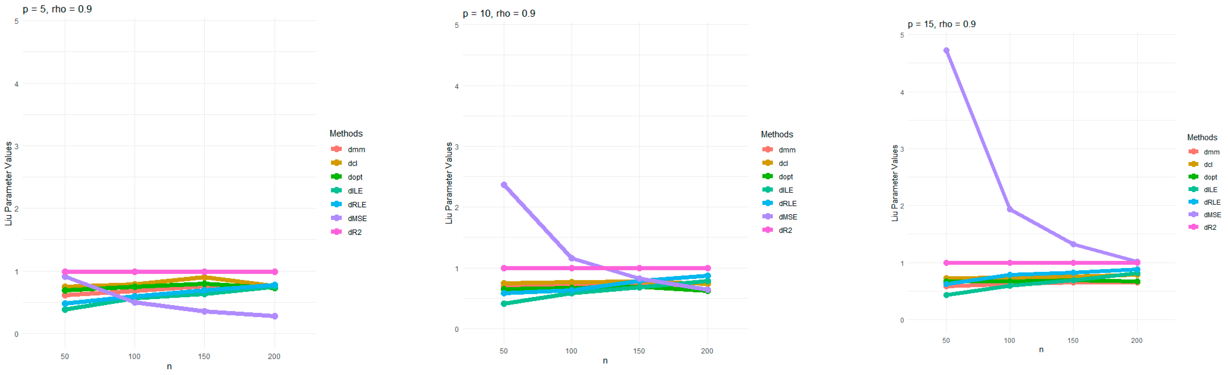
Table 4 presents the mean Liu parameters for multiple regression models with low (0.1) and high (0.9) Toeplitz correlation, comparing various methods and sample sizes across different numbers of independent variables. For low correlations, Liu parameters were relatively stable across methods as sample size increases. However, for high correlations, methods including dRLE and dILE showed significant increases in their Liu parameters as sample sizes and independent variables increased, particularly at higher independent variables. Methods like dCp and dMSE also exhibited higher Liu parameters with larger independent variables and correlation values. Overall, dRLE and dILE tended to perform best, especially when correlation was high, while dmm, dopt, and dcl showed less variation across different sample sizes. For a better understanding, we have plotted the Liu parameters for just dmm, dcl, dopt, dILE, dRLE, dMSE, and dR2 for multicollinearity 0.1 and 0.9 in Figure 1 and Figure 2, respectively.
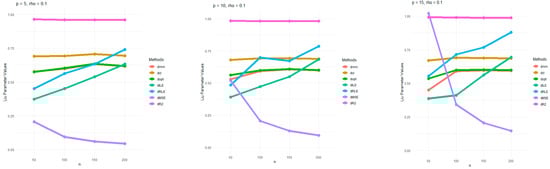
Figure 1.
Estimated Liu parameter values for p = 5, 10, and 15, and the level of correlation at 0.1.
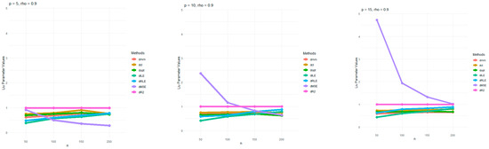
Figure 2.
Estimated Liu parameter values for p = 5, 10, and 15, and the level of correlation at 0.9.
The Liu parameters based on dmm, dcl, dopt, dILE, dRLE, and dR2 demonstrated stable values in all situations, as shown in Figure 1 and Figure 2. Furthermore, the dMSE decreased when sample sizes increase, especially at high correlation. In contrast, the dmm, dcl, dopt, dILE, and dRLE closely followed the Liu parameter in high correlation. The other Liu parameters differ edslightly for dmm, dcl, dopt, dILE, and dRLE. The modified Liu parameters (dR2) were close to stable values of 1 in all cases.
4. Application in Actual Data
We employed Liu regression to distinguish between blood donors’ laboratory values and patients’ ages using the Hepatitis C patients dataset sourced from UCI Machine Learning. This dataset was retrieved from https://archive.ics.uci.edu/dataset/503/hepatitis+c+virus+hcv+for+egyptian+patients (accessed on 26 September 2024). and contained 589 records. The dependent variable was the age of the patients and independent variables included albumin (ALB), total protein (PROT), cholinesterase (CHE), cholesterol (CHOL), alkaline phosphatase (ALP), alanine aminotransferase (ALT), creatinine (CREA), bilirubin (BIL), aspartate aminotransferase (AST), and gamma-glutamyl transferase (GGT).
For checking multicollinearity data, Pearson’s correlation analysis was employed to ascertain any potential relationships among the ten continuous independent variables—the Pearson’s correlation coefficients of the independent variables are listed in Table 5 and illustrated in Figure 3. The null hypothesis stated that there was no relationship between the two variables, and the alternative hypothesis assessed the significance of these relationships. A p-value below 0.05 for the t-statistics signified a rejected null hypothesis and meant a significant relationship between the two variables, as demonstrated in Table 5.
Table 5.
Pearson correlation matrix for the relationships between ten independent variables.
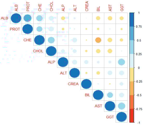
Figure 3.
Correlation graph for the ten independent variables.
Our findings showed that a moderately significant relationship, such as between 0.41–0.6, was observed in most cases. A weak level of considerable relationship was evident in some instances, such as between 0.2 and 0.4. Most of the independent variables exhibited a significant relationship, with the exceptions being between total protein (PROT) and alkaline phosphatase (ALP), alanine aminotransferase (ALT), creatinine (CREA), bilirubin (BIL), aspartate aminotransferase (AST), and gamma-glutamyl transferase (GGT).
The computed Pearson correlation matrix displaying different colors in Figure 3, derived from Table 5, utilizes varying shades to enhance clarity. Light shading indicates moderate correlations, while dark shading represents strong correlations. Most of the independent variables are depicted with moderate and light shading, suggesting inter-variable correlations or multicollinearity issues. The data from the entire dataset were divided into 70% training and 30% testing data and then randomly sampled. The average mean absolute percentage errors shown in Table 6 were computed using OLS, ridge regression, and eight Liu parameters with three scale options by generating 1000 replications testing all datasets. The selection of sample sizes of 50, 100, 150, and 200 mirrored those in the simulation data.
Table 6.
The average mean absolute percentage error was estimated on samples sizes of 50, 100, 150, 200, and 589.
Table 6 reveals that the modified Liu parameters (dMSE and dR2) exhibited consistent and often superior accuracy prediction across all scenarios. The dMSE and dR2 methods notably demonstrated commendable estimation with all sample sizes, better than the original method using OLS and ridge regression. Consequently, the Liu parameter adjustment using the dMSE and dR2 methods for ten independent variables consistently surpassed expectations and aligned closely with the simulation outcomes. Although there were slight discrepancies in estimation when the sample sizes increased, substantial performance enhancements were evident with small sample sizes from within the Hepatitis C dataset. Using a large sample size is more efficient than using an entire dataset, both in estimation accuracy and processing time.
5. Discussion
The simulated results presented in Table 1, Table 2, Table 3 and Table 4 revealed that the mean average percentage error was affected by the number of independent variables and the sample size. The modified Liu estimator (dR2) exhibited superior performance with all independent variables, correlation levels, and sample sizes, whereas dMSE slightly differed from dR2. However, the mean average percentage error for the significant independent variables was lower than that for the smaller independent variables. The increase in the correlation coefficient had a weak impact on the estimation in most methods, as indicated by the slight variation in the mean average percentage error.
In the same direction, the real data results in Table 6 showcase that the proposed Liu parameters (dMSE and dR2) achieved the smallest mean average percentage error for the datasets with eight independent variables. It was observed that the real data’s independent variables exhibited skewed distributions, as illustrated in Figure 4, confirmed by the Shapiro–Wilk test [27], indicating non-normality. Altukhaes et al. [28] introduced robust Liu estimators to combat multicollinearity and outlier problems in the linear regression model. So, the dCp effectively estimated large sample sizes using the center option. Notably, the discrepancy between the simulated and real data results emphasized the importance of considering the data source when selecting the Liu parameter.
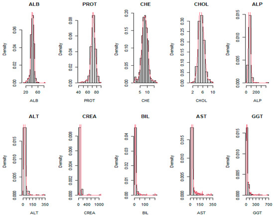
Figure 4.
The histogram of ten independent variables.
The proposed Liu parameters (dMSE and dR2) emerged as the most suitable for the estimator. Medical datasets are widely used to enhance predictive medical diagnosis patient classification. However, the Hepatitis C dataset used was a medical dataset indicating the patients’ ages, representing the multiple regression model with the multicollinearity problem among the independent variables. Oladapo et al. [29] introduced a novel modified Liu ridge-type estimator for estimating parameters in the general linear model, employing Portland cement data as a case study akin to medical data. Their proposed estimator demonstrated superior performance under certain conditions. Baber et al. [23] adapted Liu estimators to address multicollinearity issues in linear regression, utilizing tobacco data, advocating for adoption of these new estimators by practitioners facing high to severe multicollinearity among independent variables. Hammond et al. [30] employed a Liu estimator for inverse Gaussian regression, tackling multicollinearity in chemistry datasets. While considering the Liu estimator for addressing multicollinearity based on multiple regression, the proposed Liu estimator outperformed the other. In summary, we recommend the Liu estimator using the modified Liu parameter for high multicollinearity.
The modified Liu parameters have some critical limitations and challenges. These methods require more processing power and time than traditional methods, which could be problematic for large-scale applications or users with limited computing resources. Furthermore, the risk of overfitting might be too closely tailored to the specific datasets used in the study, leading to good performance on those datasets but poor performance on new, unseen data. More testing on diverse datasets is needed to ensure the methods do not lead to overfitting.
6. Conclusions
This paper introduces a Liu parameter designed to enhance the estimation of the Liu estimator in multiple regression models affected by multicollinearity among independent variables. The selection of this Liu parameter was carefully examined and compared to other methods to determine its effectiveness. Simulation studies demonstrated that the modified Liu parameter based on R-squared consistently achieved the lowest mean absolute percentage error, particularly in the scaled option, outperforming alternative approaches. Sample size, the number of independent variables, and correlation levels influenced the Liu parameter. Specifically, smaller sample sizes and more independent variables contributed to efficient estimators. Additionally, correlation levels significantly impacted the Liu parameter, with small correlations showing positive effects and large correlations leading to higher values. Furthermore, the modified Liu parameter outperformed the ordinary least squares method in simulation and real data scenarios. This Liu parameter substantially improves the estimator, especially in regression models with multicollinearity at varying correlation levels. As a result, utilizing a Liu parameter within the zero range is recommended, which can consistently provide the most accurate estimation.
Accurate estimation of correlation structures within the data is crucial to enhancing the reliability of the proposed methods. However, this can be challenging in practice, mainly when dealing with noisy, incomplete, outlier datasets, which may affect the overall performance of the methods. Therefore, further research should be conducted to address these estimation challenges.
Funding
This work was financially supported by King Mongkut’s Institute of Technology Ladkrabang [2567-02-05-010].
Data Availability Statement
Data are available at https://docs.google.com/spreadsheets/d/1IEsYNzOf15upAhCpn_5FpOdnC8Sa1drG/edit?gid=648769099#gid=648769099 (accessed on 21 August 2024).
Conflicts of Interest
The author declares no conflict of interest.
References
- Daoud, J.I. Multicollinearity and regression analysis. J. Phys. Conf. Ser. 2017, 949, 012009. [Google Scholar] [CrossRef]
- Shrestha, N. Detecting multicollinearity in regression analysis. Am. J. Appl. Math. 2020, 8, 39–42. [Google Scholar] [CrossRef]
- Liang, Y.; Rosen, D.V.; Rosen, T.V. On properties of Toeplitz-type covariance matrices in models with nested random effects. Stat. Pap. 2021, 62, 2509–2528. [Google Scholar] [CrossRef]
- Qi, B.; Xu, L.; Liu, X. Improved multiple-Toeplitz matrices reconstruction method using quadratic spatial smoothing for coherent signals DOA estimation. Eng. Comput. 2024, 41, 333–346. [Google Scholar] [CrossRef]
- Dawoud, I.; Abonazel, M.R.; Awwad, F.A. Modified Liu estimator to address the multicollinearity problem in regression models: A new biased estimation class. Sci. Afr. 2022, 17, e01372. [Google Scholar] [CrossRef]
- Jahufer, A. Detecting global influential observations in Liu regression model. Open J. Stat. 2013, 3, 5–11. [Google Scholar] [CrossRef]
- Karlsson, P.; Månsson, K.; Golam Kibria, B.M. A Liu estimator for the beta regression model and its application to chemical data. J. Chemom. 2020, 24, 2–16. [Google Scholar] [CrossRef]
- Liu, K. A new class of biased estimate in linear regression. Commun. Stat. Theory Methods 1993, 22, 393–402. [Google Scholar]
- Liu, X.-Q. Improved Liu Estimation in a linear regression model. J. Stat. Plan. Inference 2011, 141, 189–196. [Google Scholar] [CrossRef]
- Yang, H.; Xu, J. An alternative stochastic restricted Liu estimator in linear regression. Stat. Pap. 2009, 50, 639–647. [Google Scholar] [CrossRef]
- Hubert, M.H.; Wijekoon, P. Improvement of the Liu estimator in linear regression model. Stat. Pap. 2006, 47, 471–479. [Google Scholar] [CrossRef]
- Akdeniz, F.; Erol, H. Mean squared error matrix comparison of some biased estimators in linear regression. Commun. Stat. Theory Methods 2003, 32, 2389–2413. [Google Scholar] [CrossRef]
- Özkale, M.R.; Kaçiranlar, S. The restricted and unrestricted two-parameter estimators. Commun. Stat. Theory Methods 2007, 36, 2707–2725. [Google Scholar] [CrossRef]
- Suhail, M.; Babar, I.; Khan, Y.A.; Imran, M.; Nawaz, Z. Quantile-based estimation of Liu parameter in the linear regression model: Applications to Portland cement and US crime data. Math. Probl. Eng. 2021, 2021, 1–11. [Google Scholar] [CrossRef]
- Lukman, A.F.; Golam Kibria, B.M.; Ayinde, K.; Jegede, S.L. Modified one-parameter Liu estimator for the linear regression model. Mod. Sim. Eng. 2020, 2020, 1–17. [Google Scholar] [CrossRef]
- Hoerl, A.E.; Kennard, R.W. Ridge Regression: Biased estimation for nonorthogonal problems. Technometrics 1970, 12, 55–67. [Google Scholar] [CrossRef]
- Lukman, A.F.; Ayinde, K.; Kun, S.S.; Adewuyi, E.T. A Modified new two-parameter estimator in a linear regression model. Mod. Sim. Eng. 2019, 2019, 1–10. [Google Scholar] [CrossRef]
- Filzmoser, P.; Kurnaz, F.S. A robust Liu regression estimator. Commun. Stat. Simul. Comput. 2018, 47, 432–443. [Google Scholar] [CrossRef]
- Druilhet, P.; Mom, A. Shrinkage Structure in Biased Regression. J. Multivar. Anal. 2008, 99, 232–244. [Google Scholar] [CrossRef]
- Akdeniz, F.; Kacįranlar, S. More on the new biased estimator in linear regression. Sankhya Indian J. Stat. Ser. B 2001, 63, 321–325. [Google Scholar]
- Duran, E.R.; Akdeniz, F.; Hu, H. Efficiency of a Liu-type estimator in semiparametric regression models. J. Comput. Appl. Math. 2011, 235, 1418–1428. [Google Scholar] [CrossRef]
- Abdelwahab, M.M.; Abonazel, M.R.; Hammad, A.T.; El-Masry, A.M. Modified two-parameter Liu estimator for addressing multicollinearity in the Poisson regression model. Axioms 2024, 13, 46. [Google Scholar] [CrossRef]
- Babar, I.; Ayed, H.; Chand, S.; Suhail, M.; Khan, Y.A.; Marzouki, R. Modified Liu estimators in the linear regression model: An application to Tobacco data. PLoS ONE 2021, 16, e0259991. [Google Scholar] [CrossRef]
- Özkale, M.R.; Kaçiranlar, S. A Prediction-Oriented criterion for choosing the biasing parameter in Liu estimation. Commun. Stat. Theory Methods 2007, 36, 1889–1903. [Google Scholar] [CrossRef]
- Mallows, C.L. Some Comments on Cp. Technometrics 2012, 42, 87–94. [Google Scholar]
- Belsley, D.A. A Guide to using the collinearity diagnostics. Com. Sci. Eco. Mana. 1991, 4, 33–50. [Google Scholar] [CrossRef]
- Shapiro, S.S.; Wilk, M.P. An analysis of variance test for normality (complete samples). Biometrika 1965, 52, 591–611. [Google Scholar] [CrossRef]
- Altukhaes, W.D.; Roozbeh, M.; Mohamed, N.A. Robust Liu estimator used to combat some challenges in partially linear regression model by improving LTS algorithm using semidefinite programming. Mathematics 2024, 12, 2787. [Google Scholar] [CrossRef]
- Oladapo, O.J.; Owolabi, A.T.; Idowu, J.I.; Ayinde, K. A new modified Liu Ridge-Type estimator for the linear regression model: Simulation and application. Int. J. Clin. Biostat. Biom. 2022, 8, 1–14. [Google Scholar]
- Hammood, N.M.; Jabur, D.M.; Algamal, Z.Y. A Liu estimator in inverse Gaussian regression model with application in chemometrics. Math. Stat. Eng. Appl. 2022, 71, 248–266. [Google Scholar]


Disclaimer/Publisher’s Note: The statements, opinions and data contained in all publications are solely those of the individual author(s) and contributor(s) and not of MDPI and/or the editor(s). MDPI and/or the editor(s) disclaim responsibility for any injury to people or property resulting from any ideas, methods, instructions or products referred to in the content. |
© 2024 by the author. Licensee MDPI, Basel, Switzerland. This article is an open access article distributed under the terms and conditions of the Creative Commons Attribution (CC BY) license (https://creativecommons.org/licenses/by/4.0/).