
Stability Analysis of Anti-Periodic Solutions for Cohen–Grossberg Neural Networks with Inertial Term and Time Delays

Abstract
1. Introduction
2. Preliminaries
- For each functions are continuous bounded and satisfy for all .
- For each functions are differentiable and satisfy for all .
- The activation function satisfies the Lipschitz condition, i.e., there exist constants , such thatand there exist constants , such that .
- and for all , where T is a positive constant.
3. Main Results
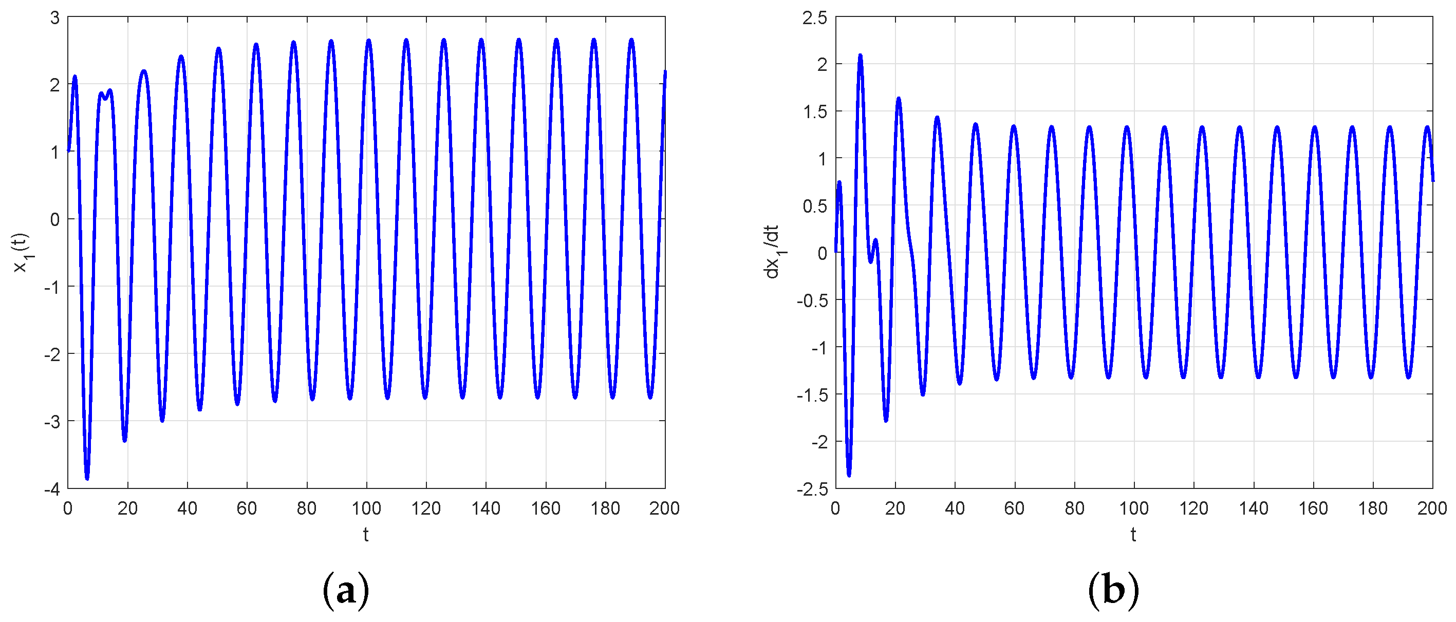
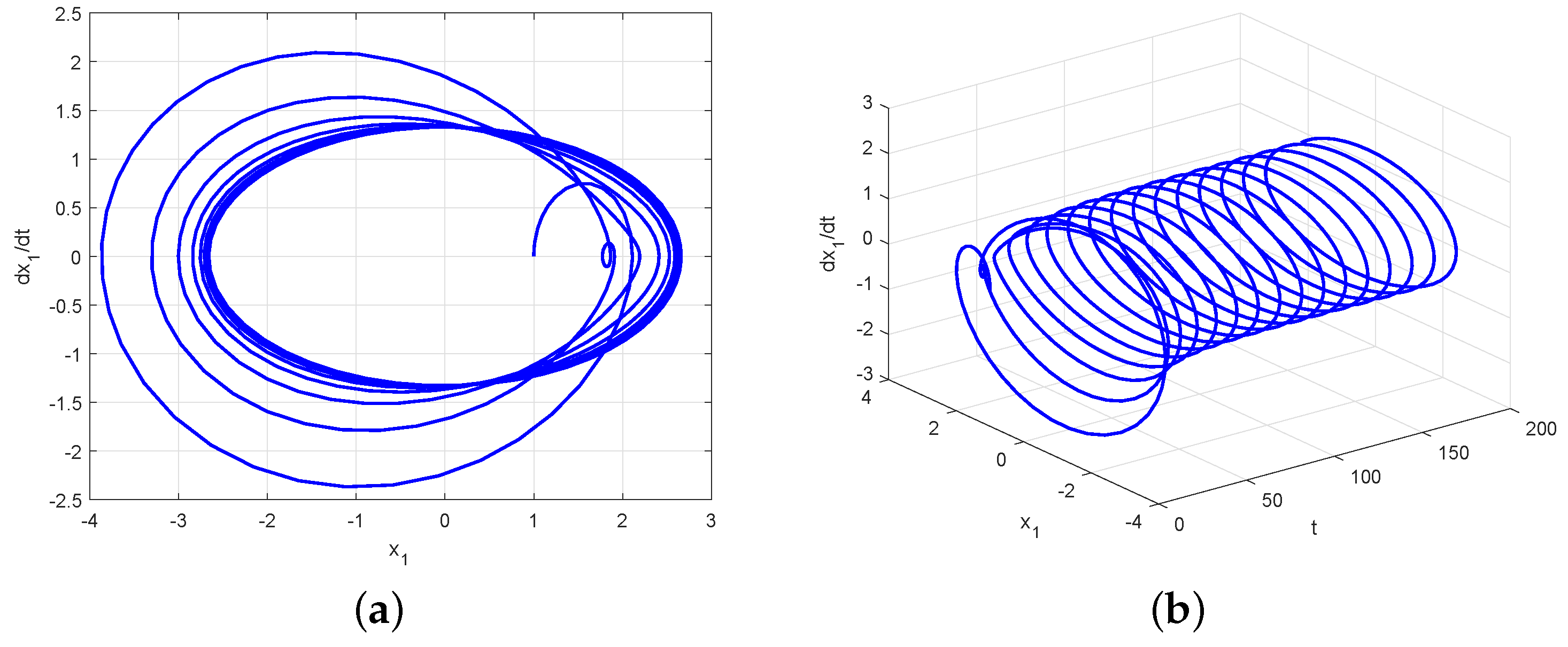
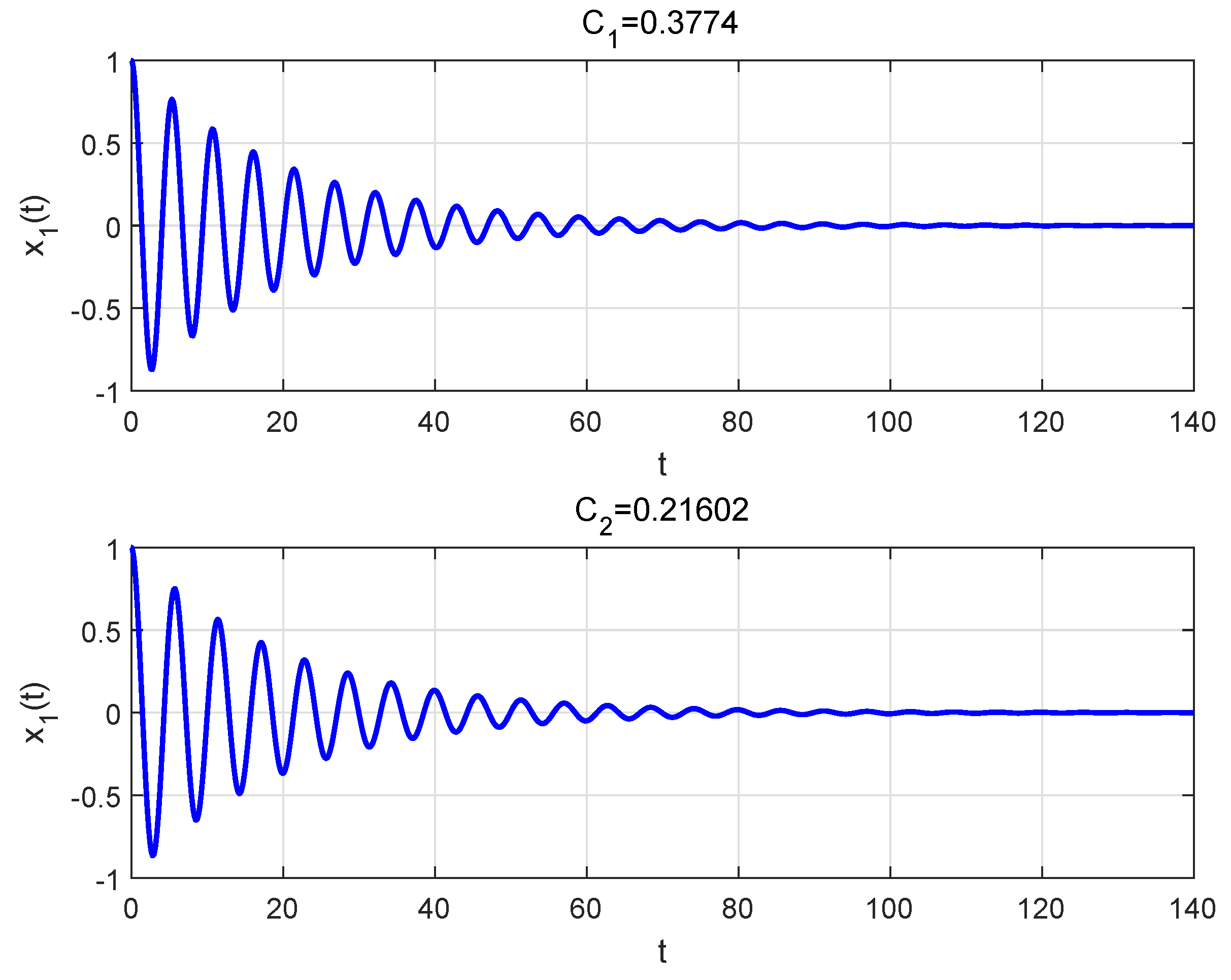
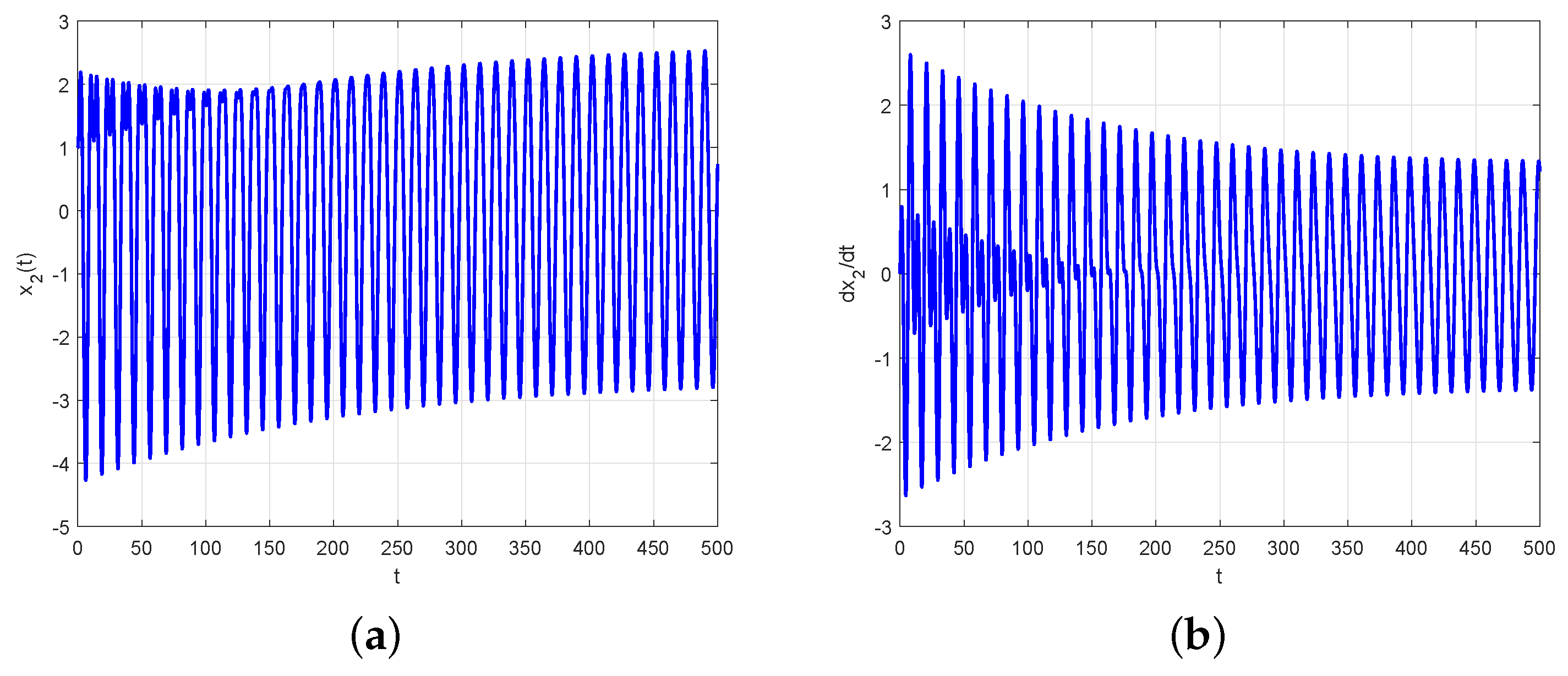
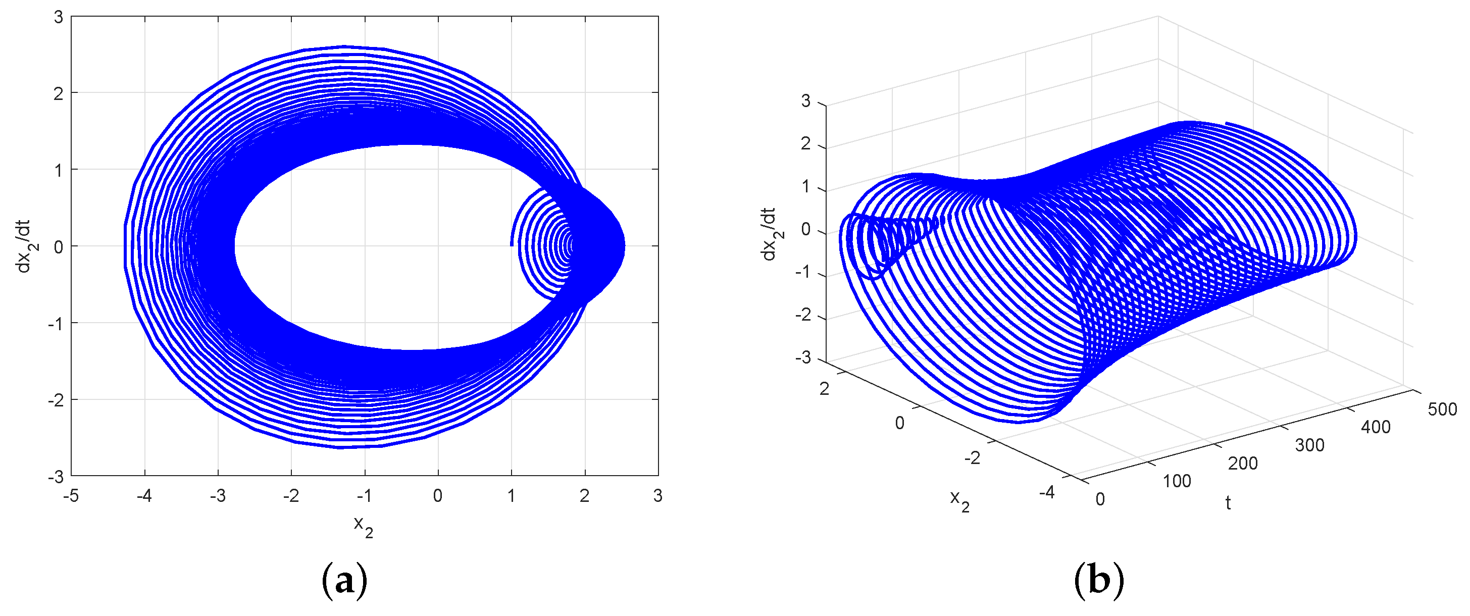
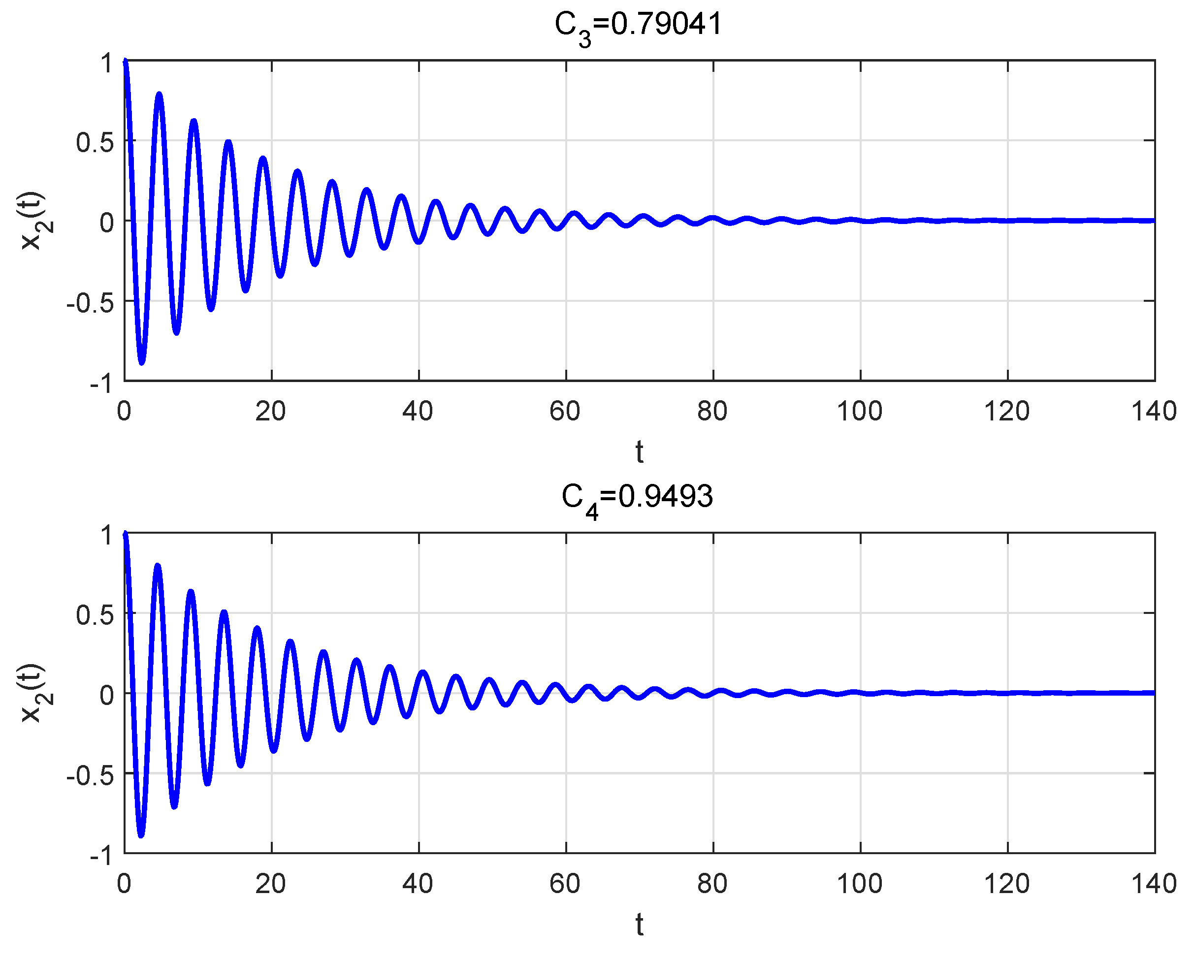
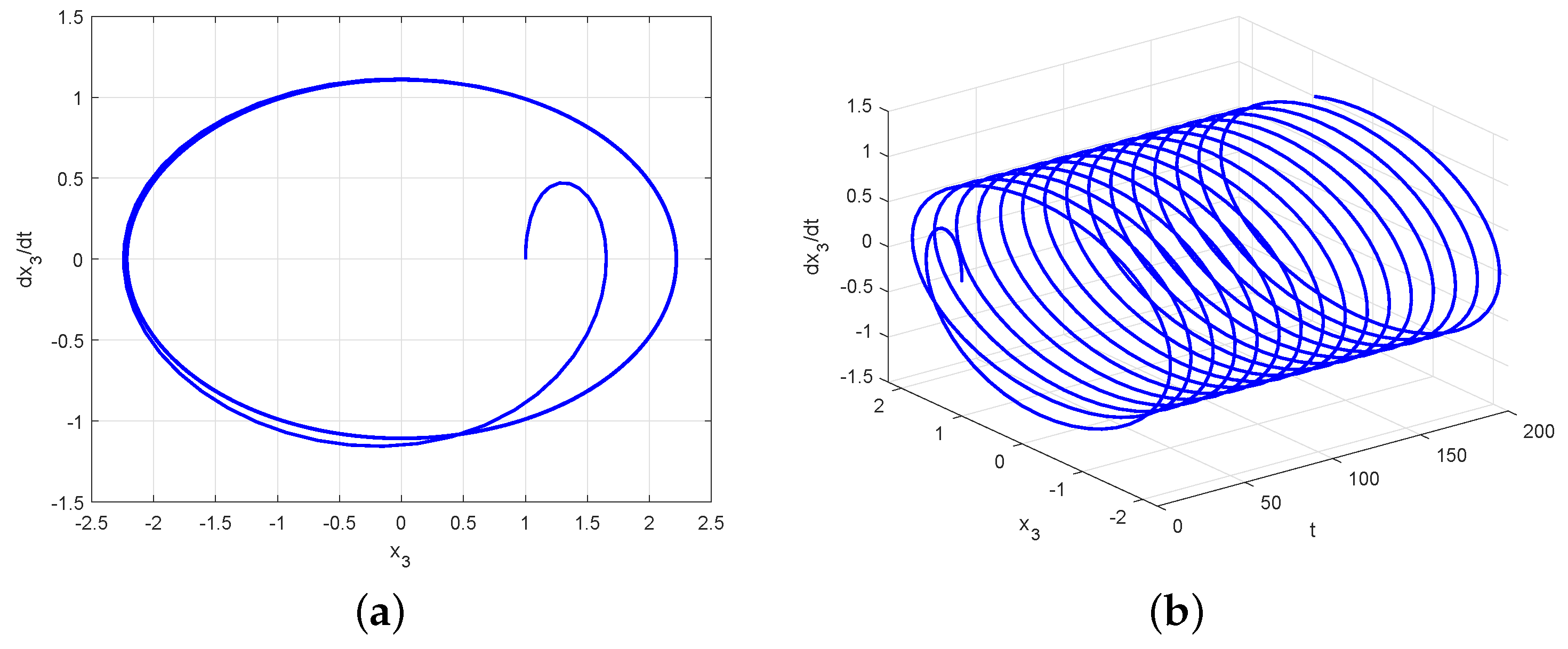
4. An Example
5. Conclusions
Author Contributions
Funding
Data Availability Statement
Acknowledgments
Conflicts of Interest
References
- Cohen, M.; Grossberg, S. Absolute stability of global pattern formation and parallel memory storage by competitive neural networks. IEEE Trans. Syst. Man Cybern. 1983, 13, 815–825. [Google Scholar] [CrossRef]
- Huang, T. Robust stability of delayed fuzzy Cohen-Grossberg neural networks. Comput. Math. Appl. 2011, 61, 2247–2250. [Google Scholar] [CrossRef]
- Gan, Q. Exponential synchronization of stochastic Cohen-Grossberg neural networks with mixed time-varying delays and reaction-diffusion via periodically intermittent control. Neur. Net. 2012, 31, 12–21. [Google Scholar] [CrossRef] [PubMed]
- Gan, Q. Adaptive synchronization of Cohen-Grossberg neural networks with unknown parameters and mixed time-varying delays. Com. Non. Sci. Num. Simu. 2012, 17, 3040–3049. [Google Scholar] [CrossRef]
- Song, Q.; Zhang, J. Global exponential stability of impulsive Cohen-Grossberg neural network with time-varying delays. Nonlinear Anal. Real World Appl. 2008, 9, 500–510. [Google Scholar] [CrossRef]
- Cao, J.; Liang, J. Boundedness and stability for Cohen-Grossberg neural networks with time-varying delays. J. Math. Anal. Appl. 2004, 296, 665–685. [Google Scholar] [CrossRef]
- Cai, Z.; Huang, L.; Wang, Z.; Pan, X.; Liu, S. Periodicity and multi-periodicity generated by impulses control in delayed Cohen-Grossberg-type neural networks with discontinuous activations. Neur. Net. 2021, 143, 230–245. [Google Scholar] [CrossRef]
- Zhang, Y.; Qiao, Y.; Duan, L.; Miao, J. Multistability of almost periodic solution for Clifford-valued Cohen-Grossberg neural networks with mixed time delays. Chaos Solitons Fractals 2023, 176, 4100–4121. [Google Scholar] [CrossRef]
- Kong, F.; Ren, Y.; Sakthivel, R. New criteria on periodicity and stabilization of discontinuous uncertain inertial Cohen-Grossberg neural networks with proportional delays. Chaos Solitons Fractals 2021, 150, 1148–1158. [Google Scholar] [CrossRef]
- Kong, F.; Zhu, Q.; Karimi, H. Fixed-time periodic stabilization of discontinuous reaction-diffusion Cohen-Grossberg neural networks. Neur. Net. 2023, 166, 354–365. [Google Scholar] [CrossRef]
- Xu, C.; Zhang, Q. Existence and exponential stability of anti-periodic solutions for a high-order delayed Cohen-Grossberg neural networks with impulsive effects. Neur. Pro. Lett. 2014, 40, 227–243. [Google Scholar] [CrossRef]
- Shi, P.; Dong, L. Existence and exponential stability of anti-periodic solutions of Hopfield neural networks with impulses. Appl. Math. Comput. 2010, 216, 623–630. [Google Scholar] [CrossRef]
- Li, Y.; Yang, L. Anti-periodic solutions for Cohen-Grossberg neural networks with bounded and unbounded delays. Commun. Non. Sci. Numer Simu. 2009, 14, 3134–3140. [Google Scholar] [CrossRef]
- Luo, D.; Jiang, Q.; Wang, Q. Anti-periodic solutions on Clifford-valued high-order Hopfield neural networks with multi-proportional delays. Neurocomputing 2022, 472, 1–11. [Google Scholar] [CrossRef]
- Gao, J.; Dai, L. Anti-Periodic synchronization of clifford-valued neutral-type cellular neural networks with D operator. J. Appl. Anal. Com. 2023, 13, 2572–2595. [Google Scholar] [CrossRef] [PubMed]
- Yo, H.; Kitajima, H. Bifurcation and stabilization of oscillations in ring neural networks with inertia. Phys. D Nonlinear Phenom. 2009, 238, 2409–2418. [Google Scholar]
- Xu, C.; Zhao, Y.; Lin, J.; Pang, Y.; Liu, Z.; Shen, J.; Qin, Y.; Farman, M.; Ahmad, S. Mathematical exploration on control of bifurcation for a plankton-oxygen dynamical model owning delay. J. Math. Chem. 2023, 20, 1–31. [Google Scholar] [CrossRef]
- Li, P.; Lu, Y.; Xu, C.; Ren, J. Insight into hopf bifurcation and control methods in fractional order BAM neural networks incorporating symmetric structure and delay. Cogni. Com. 2023, 15, 1825–1867. [Google Scholar] [CrossRef]
- Babcock, K.; Westervelt, R. Dynamics of simple electronic neural networks. Phys. D Nonlinear Phenom. 1987, 28, 305–316. [Google Scholar] [CrossRef]
- Yu, S.; Zhang, Z.; Quan, Z. New global exponential stability conditions for inertial Cohen-Grossberg neural networks with time delays. Neurocomputing 2015, 151, 1446–1454. [Google Scholar] [CrossRef]
- Ke, Y.; Miao, C. Stability analysis of BAM neural networks with inertial term and time delay. World Sci. Eng. Acad. Soc. 2011, 10, 425–438. [Google Scholar]
- Ke, Y.; Miao, C. Exponental stability of periodic solutions for inertial Cohen-Grossberg-type neural networks. Neural Netw. World 2014, 4, 377–394. [Google Scholar] [CrossRef]
- Zhao, C.; Fan, Q.; Wang, W. Anti-periodic solutions for shunting inhibitory cellular neural networks with time-varying coefficients. Neural Process. Lett. 2010, 31, 259–267. [Google Scholar] [CrossRef]
- Xu, C.; Liao, M.; Li, P.; Liu, Z.; Yuan, S. New results on pseudo almost periodic solutions of quaternion-valued fuzzy cellular neural networks with delays. Fuzzy Sets Syst. 2021, 411, 25–47. [Google Scholar] [CrossRef]
- He, Z.; Li, C.; Cao, Z.; Li, H. Periodicity and global exponential periodic synchronization of delayed neural networks with discontinuous activations and impulsive perturbations. Neurocomputing 2021, 431, 111–127. [Google Scholar] [CrossRef]
- Zhang, T.; Qu, H.; Zhou, J. Asymptotically almost periodic synchronization in fuzzy competitive neural networks with Caputo-Fabrizio operator. Fuzzy Sets Syst. 2023, 471, 76–88. [Google Scholar] [CrossRef]
- Bento, A.; Oliveira, J.; Silva, C. Existence and stability of a periodic solution of a general difference equation with applications to neural networks with a delay in the leakage terms. Commun. Nonl. Sci. Nume. Simul. 2023, 126, 7412–7429. [Google Scholar] [CrossRef]
- Mfadel, A.; Melliani, S.; Elomari, M. Existence results for anti-periodic fractional coupled systems with p-Laplacian operator via measure of noncompactness in Banach spaces. J. Math. Sci. 2023, 271, 162–175. [Google Scholar] [CrossRef]
- Gao, J.; Dai, L.; Jiang, H. Stability analysis of pseudo almost periodic solutions for octonion-valued recurrent neural networks with proportional delay. Chaos Solitons Fractals 2023, 175, 4061–4078. [Google Scholar] [CrossRef]
- Li, Y.; Wang, X. Almost periodic solutions in distribution of Clifford-valued stochastic recurrent neural networks with time-varying delays. Chaos Solitons Fractals 2021, 153, 1536–1552. [Google Scholar] [CrossRef]


Disclaimer/Publisher’s Note: The statements, opinions and data contained in all publications are solely those of the individual author(s) and contributor(s) and not of MDPI and/or the editor(s). MDPI and/or the editor(s) disclaim responsibility for any injury to people or property resulting from any ideas, methods, instructions or products referred to in the content. |
© 2024 by the authors. Licensee MDPI, Basel, Switzerland. This article is an open access article distributed under the terms and conditions of the Creative Commons Attribution (CC BY) license (https://creativecommons.org/licenses/by/4.0/).
Share and Cite
Cheng, J.; Liu, W. Stability Analysis of Anti-Periodic Solutions for Cohen–Grossberg Neural Networks with Inertial Term and Time Delays. Mathematics 2024, 12, 198. https://doi.org/10.3390/math12020198
Cheng J, Liu W. Stability Analysis of Anti-Periodic Solutions for Cohen–Grossberg Neural Networks with Inertial Term and Time Delays. Mathematics. 2024; 12(2):198. https://doi.org/10.3390/math12020198
Chicago/Turabian StyleCheng, Jiaxin, and Weide Liu. 2024. "Stability Analysis of Anti-Periodic Solutions for Cohen–Grossberg Neural Networks with Inertial Term and Time Delays" Mathematics 12, no. 2: 198. https://doi.org/10.3390/math12020198
APA StyleCheng, J., & Liu, W. (2024). Stability Analysis of Anti-Periodic Solutions for Cohen–Grossberg Neural Networks with Inertial Term and Time Delays. Mathematics, 12(2), 198. https://doi.org/10.3390/math12020198