On the Construction of 3D Fibonacci Spirals

Abstract

The paper aims to extend the classical two-dimensional (2D) Fibonacci spiral into three-dimensional (3D) space by using geometric constructions starting from cubic Fibonacci identities and relying on affine maps and parametrizations of the curves. We have already performed a comprehensive survey of cubic Fibonacci identities, which, to our surprise, uncovered only a handful of homogenous cubic identities. Obviously, the goal here is to show how one could use a particular homogenous cubic Fibonacci identity for generating 3D geometric designs similar in spirit to the way the classical Fibonacci spiral is built in 2D starting from a quadratic Fibonacci identity. This made us realize that for any cubic identity there are many different ways of packing cuboids, while only an insignificant fraction of those possible tilings might allow a smooth spiral-like curve to be drawn through them. After reviewing the state of the art, we present accurate details on ways to construct such 3D spirals using affine maps. We go on to prove the continuity and smoothness of such 3D spirals by giving a parametrization of the intersection of the surfaces that define the curves. Throughout the paper, we visualize the resulting 3D spirals by generating geometrically correct stereoscopic views. Finally, it is to be mentioned that the recursive 3D packing of cuboids tends to lead to fractal structures, which will need further investigations.

1. Introduction and Motivation

This paper is a surprisingly long answer to a reasonably simple question raised in Spring 2017 while the authors were chatting about the classical two-dimensional (2D) Fibonacci spiral. The question was: “Are there 3D versions of the classical 2D Fibonacci spiral?” We were expecting to find answers quickly by conducting a few searches online. Our reasoning was based on the fact that spirals have long been a topic of investigation, first described over two millennia ago with the treatise “On Spirals” of Archimedes (see [1]). An informal definition of spirals would characterize them as planar (i.e., two-dimensional, or 2D) curves starting from a given point (origin) and moving away from the origin, while also turning around the origin. Besides [1], one might also want to refer to [2], which mentions a few different spirals. The list includes three-dimensional (3D) spirals, which are mapped onto: a cylinder (helix); a sphere (rhumb line or loxodrome, Archimedean spiral, and Seiffert’s spiral); or a cone (Pappus spiral and conchospiral). None of these 3D spirals have links to the classical 2D Fibonacci spiral.

Obviously, we started by conducting extensive searches, which led us to realize that there are both artistic representations of 3D spirals linked to the Fibonacci sequence [3], as well as mathematical generalizations to 3D, which we will briefly mention in the state-of-the-art section (see also [4]). Still, a cubic Fibonacci identity is needed for providing a particular tiling of the 3D space using Fibonacci cuboids. The earliest cubic Fibonacci identity can be traced back to 1876 [5,6] (being the only cubic one mentioned in [7]), while others were introduced in 1953 [8,9,10] and in 1968 [11], being complemented by [12,13,14] and reviewed lately in [15]. The selected cubic Fibonacci identity should be a 3D equivalent of the way the 2D classical Fibonacci spiral relies on the well-known quadratic Fibonacci identity $F_n{F}_{n+1}={\sum }_{i=0}^n{F}_i^2$, showing that a Fibonacci rectangle $F_n{F}_{n+1}$ can be tiled using Fibonacci squares $F_i^2$.

The paper will continue by formally introducing both the classical 2D Fibonacci as well as the 2D Padovan spiral (for reasons that will become clear later). Afterwards, we shall briefly go over the state of the art of 3D spirals that mention Fibonacci. These will be followed by an extension of the 2D Padovan spiral to 3D, being motivational for crafting the 3D Fibonacci spirals to be introduced and presented. These novel 3D Fibonacci spirals are closer in spirit to the classical 2D Fibonacci spiral than any other 3D version, because they rely on homogenous cubic Fibonacci identities, hence from a 3D packing of Fibonacci cuboids into a(nother) Fibonacci cuboid.

More precisely, the approach we will take is to construct 2D and 3D fractals using affine maps. The linear parts of these will be built in most cases by composing rotations and reflections, and once in a while “by hand”. By the standard technique of homogeneous coordinates, we will represent these affine maps as linear maps acting on a space of one dimension more. This enables us to compose sequences of such maps by multiplying the corresponding sequences of matrices. We will demonstrate the continuity of piecewise parametric curves using the calculus of a single variable, and, in 3D, using the cross-product. We will also use a computer algebra system (Wolfram Mathematica ver. 12.0.1.0) to find a parametrization of the intersection of two surfaces and to prove bounds on the coordinates of that curve. For visualization, we will rely on standard techniques to generate geometrically correct stereoscopic views of 3D curves suitable for convergent viewing (as is common for the visualization of chemical structures of molecules [16]).

Conclusions and further directions for research will end the paper.

2. Two 2D Spirals

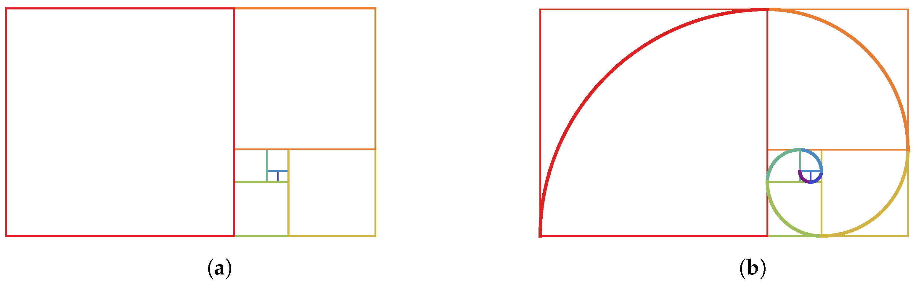
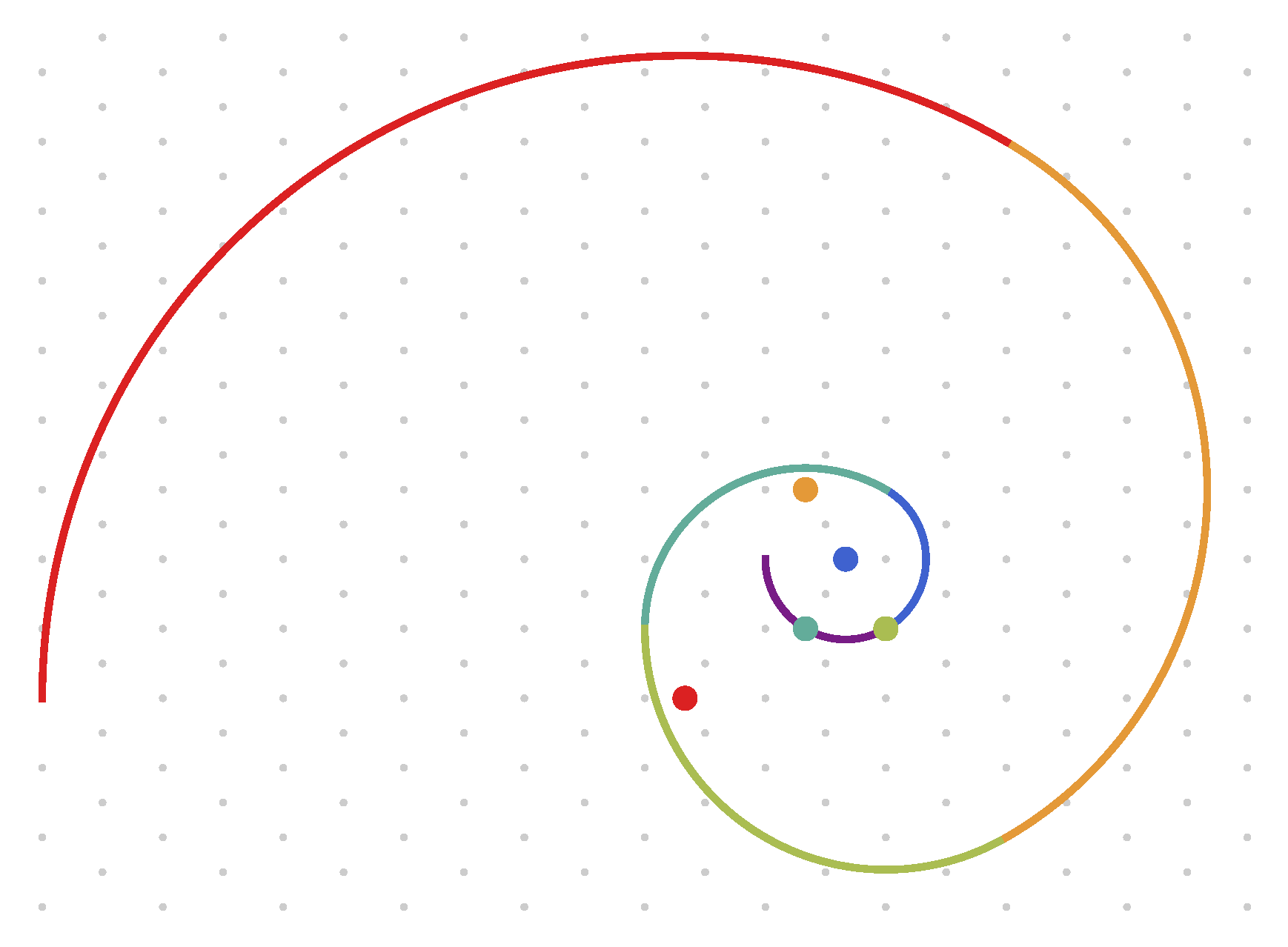
2.1. The Classical 2D Fibonacci Spiral

One of the most well-known sequences of numbers was presented by Leonardo di Pisa in his Liber abaci [17,18]. The Fibonacci sequence [3] is

$${\left(F_n\right)}_{n\ge 0}=(0,1,1,2,3,5,8,\dots ),$$

(1)

defined by $F_0=0$, $F_1=1$, and a homogenous second-order recurrence relation

$$F_n=F_{n-1}+F_{n-2}$$

(2)

for $n=2,3,4,\dots$. This sequence started to be intensively studied from the late 1800s, when it was also called Lamé’s sequence [5,6]. The scientific attraction has been proven by many subsequent publications analyzing its properties and identities as well as its relation to other sequences, e.g., Lucas and Pell. The interested reader might want to consult two earlier books from the mid-1990s [19,20], as well as two others from the early 2000s [21,22]. The scientific appeal has never waned—in fact, the contrary is true—as quite a few generalizations as well as plenty of applications in science and engineering are still being discovered and investigated (see [23,24]).

Many have studied identities involving Fibonacci numbers, the first ones being published in 1680 by Cassini [25], with many following through the 1950s [20], 1960s [26], and 1970s [19], while two books are worth mentioning [21,22]. Some of these identities have been linked to 2D geometrical representations, starting from the 1970s [27,28,29,30] till the mid-1990s [31,32]. Certainly, the best known geometrical example is a tiling of the 2D plane with successive Fibonacci squares (i.e., squares with sides equal to the Fibonacci numbers). If this is carried out by placing the squares in a particular “spiraling” way, shown in Figure 1a, the classical 2D Fibonacci spiral presented in Figure 1b is the result of connecting successive quarter circles inside these Fibonacci squares.

As already mentioned, it is the following quadratic Fibonacci identity

$$F_n{F}_{n+1}=\sum _{i=0}^n{F}_i^2$$

(3)

that leads to the 2D tiling at the heart of the classical 2D Fibonacci spiral. This identity has been known at least since 1876, when it was presented by Lucas [5], and has been the starting point for many other Fibonacci identities (see [19,20], as well as the books already mentioned [21,22]). Obviously, (3) leads to tiling an $F_n\times F_{n+1}$ rectangle with $n+1$ squares $F_i\times F_i$ ($i=0,1,...,n$). One possible option is that presented in Figure 1a. The 2D Fibonacci spiral stems from connecting quarter circles inside each and every square (Figure 1b).

Other 2D tilings based on (3) are also possible [27] (see also [33,34]), but cannot be used to generate spirals. While almost everybody is familiar with the classical 2D Fibonacci spiral, taking it for granted, this spiral implicitly hints to several steps that should be taken:

• Rely only on 2D tiles having Fibonacci number sides (squares, rectangles, etc.);
• i = Identify a (particular) quadratic Fibonacci identity that reveals a covering of the 2D space (there are plenty of quadratic Fibonacci identities including squares $F_i^2$ and/or rectangles $F_i{F}_{i+j}$);
• Select a favorable way of tiling the space, i.e., a particular ordering and placement of the square and rectangular tiles (corresponding to the quadratic Fibonacci identity selected);
• Use a smooth curve to connect through (and/or around) these tiles.

It is to be mentioned that this 2D classical Fibonacci spiral is an approximation of the golden spiral, a logarithmic spiral with a growth ratio equal to the golden ratio $\phi =\frac{1+\sqrt{5}}{2}$ (see [35]).

We present a(nother) very simple example showing that other 2D Fibonacci spirals can easily be designed. Let us start from the following quadratic Fibonacci identity:

$$F_{n+1}^2=\sum _{i=0}^n{F}_i{F}_{i+1}$$

(4)

(valid only for odd values of n). In this case, we are using rectangles $F_i{F}_{i+1}$ to cover a square $F_{n+1}^2$. Drawing quarter ellipses (instead of quarter circles) inside each and every $F_i{F}_{i+1}$ rectangle generates a “compressed” 2D Fibonacci spiral (see Figure 2).

The fact that the circles have to be replaced by ellipses also suggests that any other smooth curve would also work. One natural generalization in this case is represented by squircles (in between a circle and a square), which include superellipses (https://mathworld.wolfram.com/Superellipse.html (accessed on 4 January 2024)):

$${\left|\frac{x-x_0}{r_x}\right|}^p+{\left|\frac{y-y_0}{r_y}\right|}^p=1.$$

(5)

These lead to the strange 2D Fibonacci spirals presented in Figure 3 (including the classical 2D Fibonacci spiral).

We now turn our attention to the classical 2D Fibonacci spiral (Figure 1b) and detail our approach for constructing it using affine maps. Let $S={\{0,1\}}^2$ denote the coordinates of the vertices of the unit square, and let $\overrightarrow{r}$ be the circular arc parametrized by $\overrightarrow{r}\left(t\right)={(1+cost,1+sint)}^T,\pi \le t\le 3\pi /2$.

We define a sequence of frames of reference for ${\mathbb{R}}^2$, each one comprising an origin point and a pair of orthogonal vectors, such that for all n, S and r are the coordinates of the vertices of the nth square and the parametrization of the nth circular arc in the classical picture, with respect to the nth frame of reference. We describe these frames of reference by setting the 0th one equal to the standard orthonormal frame of reference for ${\mathbb{R}}^2$ and by prescribing a sequence ${\left(A_n\right)}_{n\ge 0}$ of affine maps such that the nth affine map transforms the nth frame of reference into the $(n+1)$st frame of reference. More precisely, for $n=0,1,2,\dots$, we have $A_n\left(\overrightarrow{v}\right)=M_n\overrightarrow{v}+{\overrightarrow{b}}_n$, where $A_n\left(S\right)$ gives the coordinates of the $(n+1)$st square with respect to the nth frame of reference, and similarly for the circular arcs. Note that, in the present case, the $(n+1)$st square can be obtained from the nth by an appropriate scaling and rotation (by $\pi /2$ radians anticlockwise), followed by a horizontal translation (by an appropriate distance), which implies that $M_0=I_2$, the identity on ${\mathbb{R}}^2$, ${\overrightarrow{b}}_0={(0,0)}^T$,

$$\begin{array}{cc}\hfill M_n& =\left(\begin{array}{cc}cos\pi /2& -sin\pi /2\\ sin\pi /2& cos\pi /2\end{array}\right)\left(\begin{array}{cc}{F}_{n+1}/F_n& 0\\ 0& F_{n+1}/F_n\end{array}\right)\hfill \end{array}$$

(6)

$$\begin{array}{cc}\hfill & =\left(\begin{array}{cc}0& -F_{n+1}/F_n\\ F_{n+1}/F_n& 0\end{array}\right)\mathrm{and}\hfill \end{array}$$

(7)

$$\begin{array}{cc}\hfill {\overrightarrow{b}}_n& =\left(\begin{array}{c}1+F_{n+1}/F_n\\ 0\end{array}\right).\hfill \end{array}$$

(8)

Setting $B_n=A_0\circ A_1\circ \cdots \circ A_n$ for $n=0,1,2,\dots$, it follows that the sequence of images ${\left(B_n\left(S\right)\right)}_{n\ge 0}$ of the unit square is the classical tiling of ${\mathbb{R}}^2$ by squares with sides equal to successive Fibonacci numbers, and the sequence of arcs ${\left(B_n\left(\overrightarrow{r}\left(t\right)\right)\right)}_{n\ge 0}$, $\pi \le t\le 3\pi /2$, is inscribed in those squares as in the classical 2D tiling. Note that the join of the arcs is continuous, and the direction of the tangent vector varies smoothly throughout the join, while its length is piecewise constant on each arc, with discontinuities at the joins (in fact, at their endpoints, the arcs are all tangential to the coordinate directions; see Figure 1b).

We implement the affine maps on ${\mathbb{R}}^2$ as linear maps on ${\mathbb{R}}^{2+1}$ in a standard way by first embedding ${\mathbb{R}}^2$ as the plane $z=1$ in ${\mathbb{R}}^3$, then applying a sequence of linear maps corresponding to the desired affine maps, and finally projecting onto the first two coordinates. This allows us to represent the concatenation of the affine maps on ${\mathbb{R}}^2$ by the multiplication of the matrices representing the corresponding linear maps on ${\mathbb{R}}^3$. The procedure is

$${(x,y)}^T\mapsto {(x,y,1)}^T\mapsto {(x_n,y_n,1)}^T=B_0{B}_1\cdots B_n{(x,y,1)}^T\mapsto {(x_n,y_n)}^T,$$

(9)

where

$$B_n=\left(\begin{array}{cc}{M}_n& {\overrightarrow{b}}_n\\ 00& 1\end{array}\right),\mathrm{for}\mathrm{all}n\ge 0.$$

(10)

The case of Figure 2 is similar to that of Figure 1 except that $M_0=\left(\begin{array}{cc}0& -1\\ 1& 0\end{array}\right)$, ${\overrightarrow{b}}_0={(0,0)}^T$, and for $n=1,2,3,\dots$

$$\begin{array}{cc}\hfill M_n& =\left(\begin{array}{cc}0& -F_{2\lfloor (n+1)/2\rfloor +1}/F_{2\lfloor (n+1)/2\rfloor }\\ F_{2\lfloor (n+2)/2\rfloor }/F_{2\lfloor n/2\rfloor +1}& 0\end{array}\right)\mathrm{and}\hfill \end{array}$$

(11)

$$\begin{array}{cc}\hfill {\overrightarrow{b}}_n& =\left(\begin{array}{c}{F}_{2\lfloor (n+3)/2\rfloor }/F_{2\lfloor (n+1)/2\rfloor }\\ 0\end{array}\right).\hfill \end{array}$$

(12)

Remark 1.

We use this method throughout this article, in particular embedding ${\mathbb{R}}^3$ in ${\mathbb{R}}^4$ in the same way for the 3D objects. In each case, from now on, we need only specify the coordinates of the shapes and the parametrizations of the curves, the matrices $M_n$, and the vectors ${\overrightarrow{b}}_n$.

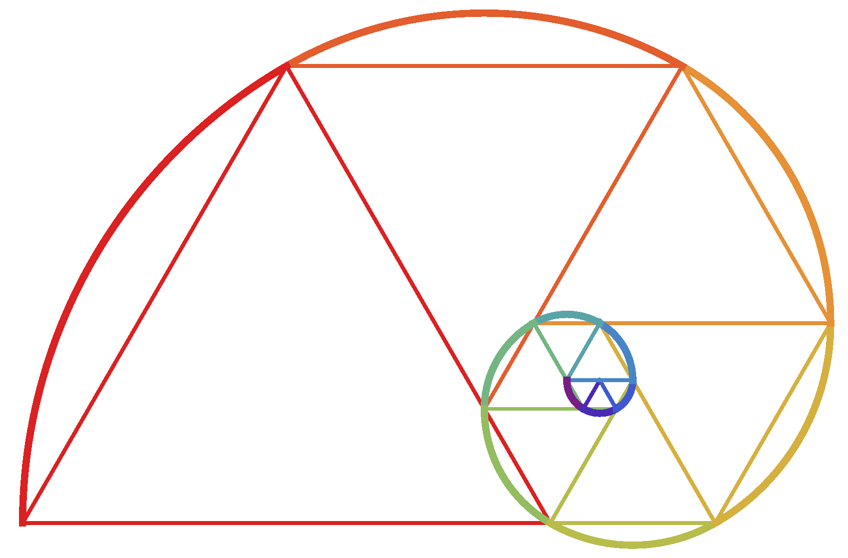
2.2. The Classical 2D Padovan Spiral

The reason we are including here the Padovan sequence [36] and the associated 2D Padovan spiral will become clear later when transitioning to 3D spirals. The Padovan sequence was named after Richard Padovan, who mentioned it in 1994 [37] and credited it to Hans van der Laan around 1928 (see also [38]). This sequence was also mentioned in 1993 by Ervin M. Wilson [39].

The Padovan sequence

$${\left(P_n\right)}_{n\ge 0}=(1,0,0,1,0,1,1,1,2,2,3,4,5,\dots )$$

(13)

is defined by a shifted version of the Fibonacci recurrence relation (Equation (2)), namely

$$P_n=P_{n-2}+P_{n-3}$$

(14)

for $n=3,4,5,\dots$, together with the initial conditions $P_0=1$, $P_1=P_2=0$.

By placing equilateral triangles with sides equal to the Padovan numbers (starting from $n=5$) in a spiraling sequence, a 2D Padovan spiral (see Figure 4) similar to the 2D Fibonacci spiral can be generated (see [40]). Like the classical 2D Fibonacci spiral, this is also a logarithmic spiral whose growth factor is given by the ratio of two consecutive Padovan numbers $P_{n+1}/P_n$, which tends to approximately $1.324717$ (see [39,41]).

Let T be an equilateral triangle of unit side length, with vertices $(0,0),(-1/2,-\sqrt{3}/2)$ and $(-1,0)$, and let $\overrightarrow{r}$ be the circular arc parametrized by $\overrightarrow{r}\left(t\right)={(cost,sint)}^T,\pi \le t\le 4\pi /3$. Taking $M_0=I_2$, and letting ${\overrightarrow{b}}_0$ be the zero vector in ${\mathbb{R}}^2$, we have

$$\begin{array}{cc}\hfill M_n& =\left(\begin{array}{cc}cos\pi /3& -sin\pi /3\\ sin\pi /3& cos\pi /3\end{array}\right)\left(\begin{array}{cc}{P}_{n+5}/P_{n+4}& 0\\ 0& P_{n+5}/P_{n+4}\end{array}\right)\hfill \end{array}$$

(15)

$$\begin{array}{cc}\hfill & =\frac{P_{n+5}}{P_{n+4}}\left(\begin{array}{cc}\frac{1}{2}& -\frac{\sqrt{3}}{2}\\ \frac{\sqrt{3}}{2}& \frac{1}{2}\end{array}\right)\mathrm{and}\hfill \end{array}$$

(16)

$$\begin{array}{cc}\hfill {\overrightarrow{b}}_n& =\left(\frac{P_{n+5}}{P_{n+4}}-1\right)\left(\begin{array}{c}cos\pi /3\\ sin\pi /3\end{array}\right)=\left(\frac{P_{n+5}}{P_{n+4}}-1\right)\left(\begin{array}{c}\frac{1}{2}\\ \frac{\sqrt{3}}{2}\end{array}\right),\mathrm{for}\mathrm{all}n\ge 1.\hfill \end{array}$$

(17)

Thus, we have ${\overrightarrow{r}}^{\prime }\left(t\right)={(-sint,cost)}^T$, $\pi \le t\le 4\pi /3$. Denoting by $\overrightarrow{s}\left(t\right)$ the $(n+1)$st arc in terms of the nth frame of reference, we know that $\overrightarrow{s}\left(t\right)=M_n\overrightarrow{r}\left(t\right)+{\overrightarrow{b}}_n$ and ${\overrightarrow{s}}^{\prime }\left(t\right)=M_n{\overrightarrow{r}}^{\prime }\left(t\right)$ for $\pi \le t\le 4\pi /3$. Hence, $\overrightarrow{s}\left(\pi \right)={(-1/2,-\sqrt{3}/2)}^T=\overrightarrow{r}(4\pi /3)$, as required, and ${\overrightarrow{s}}^{\prime }\left(\pi \right)=\frac{P_{n+5}}{P_{n+4}}{(\sqrt{3}/2,1/2)}^T=\frac{P_{n+5}}{P_{n+4}}{\overrightarrow{r}}^{\prime }(4\pi /3)$, so that ${\overrightarrow{s}}^{\prime }\left(\pi \right)$ and ${\overrightarrow{r}}^{\prime }(4\pi /3)$ are parallel, as required.

3. State of the Art of 3D Fibonacci Spirals

Our searches showed that extensions of the classical 2D Fibonacci spiral to 3D have stirred both the imagination of artists/architects as well as the interest of scientists/mathematicians. That is why we will briefly go over some of the main lines of thought coming from both of these two different communities. It will become clear that there is no consensus on what exactly a 3D Fibonacci spiral entails, and that several different ways of evolving a 3D Fibonacci spiral from the classical 2D one have been suggested and investigated.

3.1. Artistic Views on 3D Fibonacci Spirals

Most of the artistic approaches have tried to evolve the 2D Fibonacci spiral into 3D versions by designing 3D structures using cubes with sides equal to Fibonacci numbers $F_i^3$, but without any Fibonacci identity for backing the 3D structures themselves.

One of the early takes on this problem was a staircase-like design from 1969 by Anne Griswold Tyng [42] (see Figure 5). The ratio between the sides of consecutive cubes was in fact the golden ratio [43], hence approximating the Fibonacci numbers. The resulting 3D spiral linked the diagonal corners of successive cubes, while the cubes made contact only on an edge, being placed upwards starting with the largest cube and following a clockwise $\pi /2$ rotation, hence achieving a spiral staircase appearance. This 3D spiral projected (on the ground) onto a logarithmic spiral, which was an approximation of the classical 2D Fibonacci spiral. The same idea, but starting from the smallest cube, was presented by Rafael Araujo in 2015 (see https://www.acuda.net/golden-ratio-rafael-araujo/ (accessed on 4 January 2024)).

An alternate approach was incorporated in an object named “Fibonacci 3D Spiral Desk Tidy” (see https://www.thingiverse.com/thing:655990 (accessed on 4 January 2024), as well as Figure 6). It was designed by Mike Cheshire and uploaded on 28 January 2015. Similarly to the approach mentioned above, the 3D Fibonacci cubes were “grown” on the faces of the 2D Fibonacci squares (of the classical 2D Fibonacci spiral). The 3D spiral was generated by connecting two of the top corners from two successive Fibonacci cubes $F_{i-1}^3$ and $F_i^3$. This ensured that the spiral was inside the $F_i^3$ cube, and, while turning $\pi /2$ (i.e., a quarter circle, as in the case of the classical 2D Fibonacci spiral), it also moved upwards $F_{i-2}$ (i.e., the difference between $F_i$ and $F_{i-1}$). This 3D spiral was also drawn by Rafael Araujo in 2015 (see https://www.acuda.net/wp-content/uploads/2016/12/DSC9897.jpg (accessed on 4 January 2024)). Although on the website it is mentioned that “the math is not quite true as this was just a bit of fun”, the resulting 3D spiral projected onto the classical 2D Fibonacci spiral, i.e., exactly like the one drawn by Anne Griswold Tyng [42].

It is to be mentioned that in fact these two approaches are quite similar, being based on growing Fibonacci cubes $F_i^3$ from the $F_i^2$ squares of the classical 2D Fibonacci spiral. In particular, in Figure 6 all the cubes sit on the horizontal plane containing the classical 2D Fibonacci spiral, making an upward vertical step of $F_{i-2}$ per $\pi /2$ turn. In Figure 5, each cube is placed at the height of the previous cube, making an upward vertical step of $F_i$ per $\pi /2$ turn. These two variations have been used by other graphical/artistic designers.

3.2. Mathematical Generalizations towards 3D Fibonacci Spirals

A rigorous mathematical take on this problem was presented by Stakhov and Rozin [44]. They used the Binet formula to extended the Fibonacci sequence from discrete to continuous. This was achieved by inputting an arbitrary real number into the Binet formula, while the output was a complex Fibonacci number—giving rise to the Binet–Fibonacci curve [45].

One can now use hyperbolic and quasi-sine (trigonometric) functions:

$$FF\left(x\right)=\frac{{\phi }^x-cos\left(\pi x\right){\phi }^{-x}}{\sqrt{5}}$$

(18)

where $\phi =\frac{1+\sqrt{5}}{2}$ is the golden ratio mentioned above, and x is a real number. This quasi-sine Fibonacci function was considered by the authors as the projection of a 3D Fibonacci spiral that lies on a funnel-shaped surface, hence leading to

$$CFF\left(x\right)=\frac{{\phi }^x-cos\left(\pi x\right){\phi }^{-x}}{\sqrt{5}}+i\frac{sin\left(\pi x\right){\phi }^{-x}}{\sqrt{5}}.$$

(19)

By separating the real and imaginary parts as $y\left(x\right)$ and $z\left(x\right)$, one obtains

$${\left(y-\frac{{\phi }^x}{\sqrt{5}}\right)}^2+z^2={\left(\frac{{\phi }^{-x}}{\sqrt{5}}\right)}^2.$$

(20)

These continuous functions can be easily plotted, revealing a 3D spiral on a shofar-like funnel-shaped surface (see also https://math.stackexchange.com/questions/4474029/modifying-binets-formula-for-the-fibonacci-sequence-with-a-complex-offset (accessed on 4 January 2024)).

A few years later, Falcón and Plaza [46] generalized this approach to k-Fibonacci numbers, which obey the recurrence relation $F_{k,n+1}=k{F}_{k,n}+F_{k,n-1}$ for $n=1,2,3,\dots$, with $F_{k,0}=0$, $F_{k,1}=1$. This led to another continuous version of the hyperbolic function, and a quasi-sine k-Fibonacci function:

$$F{F}_k\left(x\right)=\frac{{\sigma }_k^x-cos\left(\pi x\right){\sigma }_k^{-x}}{{\sigma }_k+{\sigma }_k^{-1}}$$

(21)

where ${\sigma }_k=\frac{k+\sqrt{k^2+4}}{2}$ is the positive root of the characteristic equation associated to the k-Fibonacci sequence. The complex-valued function

$$CF{F}_k\left(x\right)=\frac{{\sigma }_k^x-cos\left(\pi x\right){\sigma }_k^{-x}}{{\sigma }_k+{\sigma }_k^{-1}}+i\frac{sin\left(\pi x\right){\sigma }_k^{-x}}{{\sigma }_k+{\sigma }_k^{-1}}$$

(22)

is called a 3D k-Fibonacci spiral, and a geometric analysis of this 3D spiral targeted its curvature and torsion [47].

In 2011, Harary and Tal looked into the logarithmic spiral, which is ubiquitous in nature [48]. They defined a 3D logarithmic spiral—where both the radius of curvature and that of torsion change linearly along the curve—and used it to model various natural objects. Like the previous two approaches, this was also a continuous version, without wanting departing from the discreteness of the Fibonacci sequence.

More recently, Parodi [49] presented a generalization of planar Fibonacci spirals using the following recurrence relation:

$$G_n=a{G}_{n-1}+b{G}_{n-2}+c{d}^n$$

(23)

for $n=2,3,4,\dots$, with $G_0$ and $G_1$ being the initial values, and a, b, c, and d being known coefficients, all of which are positive real numbers. Parodi’s paper focused on rectangular and arched spirals and presented an extension to 3D. A quadratic product difference identity was used for the generalized Fibonacci numbers and supported 2D generalized Fibonacci spirals, where quarter ellipses were used for rectangles. Unfortunately, when extending into 3D, the solution proposed was “to choose some linear increase”.

4. 3D Spirals

Before moving forward, we want to stress that the agendas of both artists/architects and scientists/mathematicians appear to have not included cubic Fibonacci identities, and the projects brought to the (design/research) table were:

• Expansion (linear) into the third dimension ([42,49]). Such approaches are simple, but unfortunately do not treat the third dimension on a par with the other two (which rely on the Fibonacci sequence).
• Extension to continuous values, either real [48] or complex (e.g., the approaches presented in [44], as well as [46,47] and [48]). Still, there is a gap between such continuous extensions and the discreteness of the Fibonacci numbers leading to cuboid tiling [26,50].

We felt that the search for a 3D Fibonacci spiral was left wanting, as none of the 3D spirals presented in the previous section relies on a Fibonacci identity describing a recurrent tiling of the 3D space. That is why we decided to perform a survey of cubic Fibonacci identities, which led to [15]. For tiling the 3D space, one can use any of the homogeneous Fibonacci cubic identities presented in Table 1 of [15]. Our original plan was to rely on a fractal packing of Fibonacci cuboids corresponding to the identity

$$F_n{F}_{n+1}^2=\sum _{k=0}^n{F}_k^3+\sum _{k=1}^n{F}_{k-1}{F}_k{F}_{k+1},$$

(24)

which was mentioned for the first time in [51] as Equation (1.15) (also presented in [52] as Equation (2)). Arranging a reasonably large number of cuboids is not an easy packing task, so the approach we took was to focus first on the cubes from (24), implying that a 3D Fibonacci spiral would go through the Fibonacci cubes (like the 2D one goes through Fibonacci squares). Different placements of these cubes are possible, and in the following we will present three alternatives leading to three different 3D Fibonacci spirals. Still, before proceeding further, we can significantly simplify Equation (24). To achieve this, we subtract a shifted version of this identity from itself, leading to

$$F_n^3+F_n{F}_{n-1}^2+F_n{F}_{n-1}{F}_{n-2}=F_{n+1}{F}_n^2.$$

(25)

This shows that a rectangular square cuboid $F_{n+1}{F}_n^2$ can be tiled by a cube $F_n^3$, another rectangular square cuboid $F_n{F}_{n-1}^2$, and a cuboid $F_n{F}_{n-1}{F}_{n-2}$, but the equation can be simplified even further:

$$\begin{array}{cc}\hfill F_n^3+F_n{F}_{n-1}\left(F_{n-1}+F_{n-2}\right)& =F_{n+1}{F}_n^2\hfill \end{array}$$

(26)

$$\begin{array}{cc}\hfill F_n^3+F_n^2{F}_{n-1}& =F_{n+1}{F}_n^2.\hfill \end{array}$$

(27)

We came full circle and realized that (27) is a most trivial homogeneous cubic identity, namely $F_n+F_{n-1}=F_{n+1}$ (Equation (2)) multiplied by $F_n^2$. It became clear that the three most trivial homogenous cubic Fibonacci identities can be generated easily by multiplying Equation (2) by the square of one of the terms

$$\begin{array}{c}\hfill F_n^3=F_n^2{F}_{n-1}+F_n^2{F}_{n-2}\end{array}$$

(28)

$$\begin{array}{c}\hfill F_n{F}_{n-1}^2=F_{n-1}^3+F_{n-1}^2{F}_{n-2}\end{array}$$

(29)

$$\begin{array}{c}\hfill F_n{F}_{n-2}^2=F_{n-1}{F}_{n-2}^2+F_{n-2}^3.\end{array}$$

(30)

Obviously, these are geometrically the simplest possible, as one cuboid is covered by two other cuboids. This process can be repeated recursively (by properly scaling), either combining the same equation/tiling, or by combining them in any arbitrary order. It is clear that the resulting cuboids will tile the original (largest) cuboid, and that a homogeneous cubic Fibonacci identity can be derived either from the 3D geometric construction (a reverse-engineering approach with respect to [50]), or by solving the composition of the equations used. This shows that a very large number of different tilings of the 3D space using Fibonacci cuboids are possible—especially as one could use different cubic identities in combination—meaning that plenty of 3D Fibonacci spirals can be envisaged.

The 3D Fibonacci spirals we will introduce in this section are generated by recursively using Equation (27) (or Equation (29), which is a shifted version), leading to (24), while the arrangements of Fibonacci cubes are quasi-self-similar fractals that will be defined by sequences of affine maps (as already mentioned). Additionally, the 3D spirals to be described in this section are constructed so as to have the same type of continuity. The only exception is the planar Padovan-like spiral embedded in 3D, a 3D spiral we start with as an introductory example. In this case, the tangent vector changes direction, where consecutive curves (actually straight-line segments) meet.

4.1. A Planar Padovan-like Spiral Embedded in 3D

A tiling based on the Padovan sequence has been suggested for 3D, see https://demonstrations.wolfram.com/PadovansSpiralNumbers (accessed on 4 January 2024). While for 2D the tiling was carried out with triangles (see Figure 4), in 3D the tiling relies on rectangular square cuboids of sides equal to the Padovan numbers, being supported by the following cubic Padovan identity:

$$P_n{P}_{n+1}{P}_{n+2}=\sum _{k=0}^n{P}_k^2{P}_{k+1}.$$

(31)

The diagonals drawn on the square faces of these rectangular square cuboids form a 3D Padovan cuboid spiral. This is made of segments, hence being a piecewise linear approximation of a 3D spiral. A smooth version is possible by making connections around the shapes, i.e., on the outside of these Padovan cuboids. Still, it should be mentioned that, upon closer inspection, this is not really a 3D spiral per se, but a 2D one embedded in 3D, as it lies on a plane [41].

We formalize this approach as presented for 2D spirals by taking $C={\{0,1\}}^3$ to denote the vertex set of the unit cube and letting $\overrightarrow{r}\left(t\right)=t{(0,0,0)}^T+(1-t){(1,0,1)}^T=(1-t){(1,0,1)}^T,0\le t\le 1$, representing a straight-line segment from the point $(1,0,1)$ to the point $(0,0,0)$. From now on, instead of constructing $M_n$ from rotations and scalings (as in the previous 2D examples), we will construct them directly. In this case, let $M_0=I_3$, ${\overrightarrow{b}}_0$ be the zero vector in ${\mathbb{R}}^3$,

$$\begin{array}{cc}\hfill M_n& =\left\{\begin{array}{cc}\left(\begin{array}{ccc}0& P_{n+6}/P_{n+4}& 0\\ -1& 0& 0\\ 0& 0& P_{n+5}/P_{n+4}\end{array}\right)\hfill & n\ge 1,n\mathrm{odd}\hfill \\ \left(\begin{array}{ccc}{P}_{n+5}/P_{n+4}& 0& 0\\ 0& 0& -1\\ 0& P_{n+6}/P_{n+4}& 0\end{array}\right)\hfill & n\ge 2,n\mathrm{even}\hfill \end{array}\right.\hfill \end{array}$$

(32)

and

$$\begin{array}{cc}\hfill {\overrightarrow{b}}_n& =\left\{\begin{array}{cc}{(0,1,-P_{n+5}/P_{n+4})}^T\hfill & n\ge 1,n\mathrm{odd}\hfill \\ {(-P_{n+5}/P_{n+4},1,0)}^T\hfill & n\ge 2,n\mathrm{even}\hfill \end{array}\right..\hfill \end{array}$$

(33)

As already mentioned above, in this case, the join of these arcs fails to be smooth at the points where consecutive arcs meet. However, it is continuous (see Figure 7). Indeed, with the same notation as before, we have $\overrightarrow{s}\left(t\right)=M_n\overrightarrow{r}\left(t\right)+{\overrightarrow{b}}_n$ and $\overrightarrow{s}\left(0\right)=\overrightarrow{r}\left(1\right)$, whether n is odd or even.

4.2. A Scaled Planar Fibonacci Spiral Embedded in 3D

Obviously, one can use the approach presented above as inspiration and adapt it to Fibonacci numbers, replacing the cubic Padovan identity (25) with a cubic Fibonacci identity. This will be our first 3D Fibonacci spiral, similar to the 3D Padovan one and obviously logarithmic, but having a growth factor of $\phi \sqrt{2}=2.288245$. Unfortunately, exactly like the 3D Padovan spiral (which is on a diagonal plane), the result is a planar 2D Fibonacci spiral embedded in 3D (see Figure 8 below). Still, this is our first step towards non-planar 3D Fibonacci spirals.

Now, let $C={\{0,1\}}^3$ as before, and let $\overrightarrow{r}\left(t\right)={(1+cost,1+cost,sint)}^T,\pi /2\le t\le \pi$, an elliptical arc from the point $(1,1,1)$ to the point $(0,0,0)$. Let $M_0=I_3$ and ${\overrightarrow{b}}_0={(0,0,0)}^T$, and let

$$\begin{array}{cc}\hfill M_n& ={(-1)}^n\left(\begin{array}{ccc}-F_{n+1}/F_n& 0& 0\\ 0& -F_{n+1}/F_n& 0\\ 0& 0& F_{n+1}/F_n\end{array}\right),n\ge 1\hfill \end{array}$$

(34)

and

$$\begin{array}{cc}\hfill {\overrightarrow{b}}_n& =\left\{\begin{array}{cc}{(0,0,0)}^T\hfill & n\ge 1,n\mathrm{odd}\hfill \\ {(1+F_{n+1}/F_n,1+F_{n+1}/F_n,1-F_{n+1}/F_n)}^T\hfill & n\ge 2,n\mathrm{even}\hfill \end{array}\right..\hfill \end{array}$$

(35)

We have ${\overrightarrow{r}}^{\prime }\left(t\right)={(-sint,-sint,cost)}^T$, $\pi /2\le t\le \pi$. With the same notation as before, we also have

$$\begin{array}{cc}\hfill \overrightarrow{s}\left(t\right)& =\left\{\begin{array}{cc}\frac{F_{n+1}}{F_n}{(1+cost,1+cost,-sint)}^T\hfill & n\ge 1,n\mathrm{odd}\hfill \\ {\left(1-\frac{F_{n+1}}{F_n}cost,1-\frac{F_{n+1}}{F_n}cost,1-\frac{F_{n+1}}{F_n}(1-sint)\right)}^T\hfill & n\ge 2,n\mathrm{even}\hfill \end{array}\right.\hfill \end{array}$$

(36)

and

$$\begin{array}{cc}\hfill {\overrightarrow{s}}^{\prime }\left(t\right)& =\left\{\begin{array}{cc}\frac{F_{n+1}}{F_n}{(-sint,-sint,-cost)}^T\hfill & n\ge 1,n\mathrm{odd}\hfill \\ \frac{F_{n+1}}{F_n}{(sint,sint,cost)}^T\hfill & n\ge 2,n\mathrm{even}\hfill \end{array}\right..\hfill \end{array}$$

(37)

It follows that

$$\begin{array}{cc}\hfill \overrightarrow{s}(\pi /2)& =\left\{\begin{array}{cc}\frac{F_{n+1}}{F_n}{(1,1,-1)}^T\hfill & n\ge 1,n\mathrm{odd}\hfill \\ {(1,1,1)}^T\hfill & n\ge 2,n\mathrm{even}\hfill \end{array}\right.\hfill \end{array}$$

(38)

and

$$\begin{array}{cc}\hfill \overrightarrow{s}\left(\pi \right)& =\left\{\begin{array}{cc}{(0,0,0)}^T\hfill & n\ge 1,n\mathrm{odd},\hfill \\ {(1+\frac{F_{n+1}}{F_n},1+\frac{F_{n+1}}{F_n},1-\frac{F_{n+1}}{F_n})}^T\hfill & n\ge 2,n\mathrm{even}\hfill \end{array}\right.\hfill \end{array}$$

(39)

Hence, $\overrightarrow{s}(\pi /2)=\overrightarrow{r}(\pi /2)$ when $n\ge 2$ and n is even, and $\overrightarrow{s}\left(\pi \right)=\overrightarrow{r}\left(\pi \right)$ when $n\ge 1$ and n is odd. Therefore, the join of consecutive arcs is continuous.

Regarding the smoothness of the joins, we know that ${\overrightarrow{s}}^{\prime }(\pi /2)={(\frac{F_{n+1}}{F_n},\frac{F_{n+1}}{F_n},0)}^T=\frac{F_{n+1}}{F_n}{\overrightarrow{r}}^{\prime }(\pi /2)$ when $n\ge 2$ and n is even, and ${\overrightarrow{s}}^{\prime }\left(\pi \right)={(0,0,\frac{F_{n+1}}{F_n})}^T=-\frac{F_{n+1}}{F_n}{\overrightarrow{r}}^{\prime }\left(\pi \right)$ when $n\ge 1$ and n is odd, as required (see Figure 8).

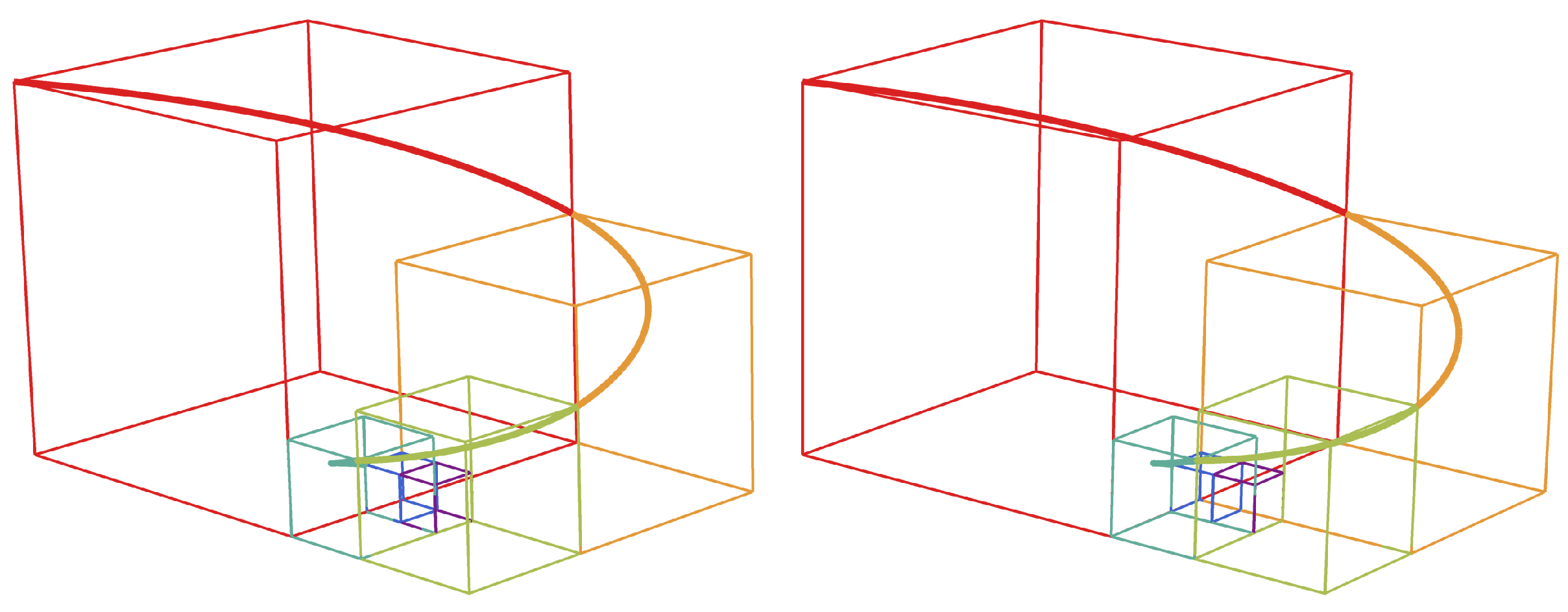
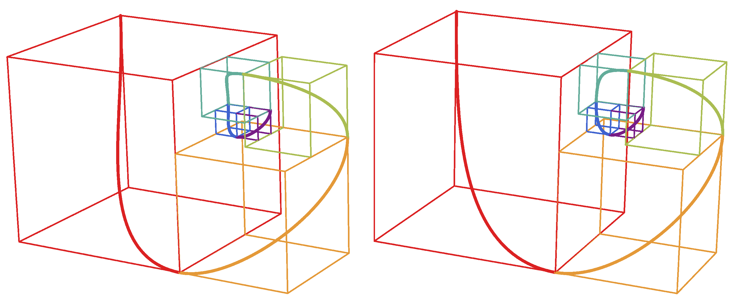
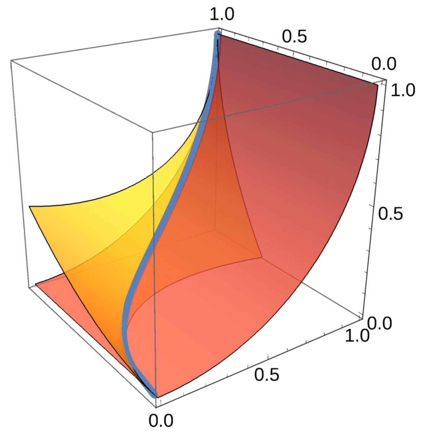
4.3. A Non-Planar 3D Fibonacci Spiral

To fit a spiral inside the unit cube that suits the fractal cube structure described in this section, we start with the planar curve ${(t,{sin}^{2}t)}^T$, $0\le t\le \pi /2$, and we wrap it around a quarter-cylinder to obtain the non-planar curve $\overrightarrow{r}\left(t\right)={({sin}^{2}t,1-cost,sint)}^T$, $0\le t\le \pi /2$ shown in Figure 9.

The fractal structure is defined by $M_0=I_3$ and ${\overrightarrow{b}}_0={(0,0,0)}^T$, and

$$\begin{array}{cc}\hfill M_n& =\left\{\begin{array}{cc}\left(\begin{array}{ccc}{F}_{n+1}/F_n& 0& 0\\ 0& F_{n+1}/F_n& 0\\ 0& 0& -F_{n+1}/F_n\end{array}\right)\hfill & n\ge 1,n\mathrm{odd}\hfill \\ \left(\begin{array}{ccc}{F}_{n+1}/F_n& 0& 0\\ 0& -F_{n+1}/F_n& 0\\ 0& 0& F_{n+1}/F_n\end{array}\right)\hfill & n\ge 2,n\mathrm{even}\hfill \end{array}\right.,\hfill \end{array}$$

(40)

while

$$\begin{array}{cc}\hfill {\overrightarrow{b}}_n& =\left\{\begin{array}{cc}{(0,0,0)}^T\hfill & n\ge 1,n\mathrm{odd}\hfill \\ {(1-F_{n+1}/F_n,1+F_{n+1}/F_n,1-F_{n+1}/F_n)}^T\hfill & n\ge 2,n\mathrm{even}\hfill \end{array}\right..\hfill \end{array}$$

(41)

One desirable feature of the resulting fractal spiral, shown in Figure 10, is that its orthogonal projection parallel to the x-axis is exactly the classical 2D Fibonacci spiral.

We have ${\overrightarrow{r}}^{\prime }\left(t\right)={(2sintcost,sint,cost)}^T$, $0\le t\le \pi /2$. Using the same notation as before, we also have

$$\begin{array}{cc}\hfill \overrightarrow{s}\left(t\right)& =\left\{\begin{array}{cc}\frac{F_{n+1}}{F_n}{({sin}^{2}t,1-cost,-sint)}^T\hfill & n\ge 1,n\mathrm{odd}\hfill \\ {\left(\frac{F_{n+1}}{F_n}({sin}^{2}t-1)+1,\frac{F_{n+1}}{F_n}cost+1,\frac{F_{n+1}}{F_n}(sint-1)+1\right)}^T\hfill & n\ge 2,n\mathrm{even}\hfill \end{array}\right.\hfill \end{array}$$

(42)

and

$$\begin{array}{cc}\hfill {\overrightarrow{s}}^{\prime }\left(t\right)& =\left\{\begin{array}{cc}\frac{F_{n+1}}{F_n}{(2sintcost,sint,-cost)}^T\hfill & n\ge 1,n\mathrm{odd}\hfill \\ \frac{F_{n+1}}{F_n}{(2sintcost,-sint,cost)}^T\hfill & n\ge 2,n\mathrm{even}\hfill \end{array}\right..\hfill \end{array}$$

(43)

It follows that

$$\begin{array}{cc}\hfill \overrightarrow{s}\left(0\right)& =\left\{\begin{array}{cc}{(0,0,0)}^T\hfill & n\ge 1,n\mathrm{odd}\hfill \\ {(1-\frac{F_{n+1}}{F_n},1+\frac{F_{n+1}}{F_n},1-\frac{F_{n+1}}{F_n})}^T\hfill & n\ge 2,n\mathrm{even}\hfill \end{array}\right.\hfill \end{array}$$

(44)

and

$$\begin{array}{cc}\hfill \overrightarrow{s}(\pi /2)& =\left\{\begin{array}{cc}\frac{F_{n+1}}{F_n}{(1,0,-1)}^T\hfill & n\ge 1,n\mathrm{odd}\hfill \\ {(1,1,1)}^T\hfill & n\ge 2,n\mathrm{even}\hfill \end{array}\right.\hfill \end{array}$$

(45)

Hence, $\overrightarrow{s}\left(0\right)=\overrightarrow{r}\left(0\right)$ for $n\ge 1$ and n odd, and $\overrightarrow{s}(\pi /2)=\overrightarrow{r}(\pi /2)$ for $n\ge 2$ and n even, which establishes that the join of the curves is continuous.

As for smoothness, when $n\ge 1$ and n is odd, we know that ${\overrightarrow{s}}^{\prime }\left(0\right)=\frac{F_{n+1}}{F_n}{(0,0,-1)}^T$, which is parallel to ${\overrightarrow{r}}^{\prime }\left(0\right)={(0,0,1)}^T$, and when $n\ge 2$ and n is even, we know that ${\overrightarrow{s}}^{\prime }(\pi /2)=\frac{F_{n+1}}{F_n}{(0,-1,0)}^T$, which is parallel to ${\overrightarrow{r}}^{\prime }(\pi /2)={(0,1,0)}^T$.

4.4. A Padovan-Style 3D Fibonacci Spiral

The orthogonal projection of this 3D spiral along a certain diagonal of the unit cube can be drawn on an isometric grid, creating a picture reminiscent of the classical 2D Padovan spiral (see Figure 4) but based on the Fibonacci sequence instead of the Padovan sequence (Figure 11).

The elementary curve is constructed as part of the intersection of two cylinders, an idea inspired by Steinmetz curves [53]. In fact, if cylinder A has radius $2\sqrt{2}/3$ and axis ${(0,2/3,4/3)}^T+r{(1,-1,-1)}^T$, and cylinder B has radius 1 and axis ${(0,0,1)}^T+s{(0,1,0)}^T$, then the intersection of cylinders A and B can be partitioned into four parts, one of which we choose and parametrize by

$$\overrightarrow{r}\left(t\right)={\left(\sqrt{2t-t^2},\frac{1}{2}\left(t-\sqrt{2t-t^2}+\sqrt{2t+(8-6t)\sqrt{2t-t^2}}\right),t\right)}^T,0\le t\le 1$$

(46)

as in Figure 12. Obviously, the x and z coordinates of (46) lie within the interval $[0,1]$. To show that the same is true of the y coordinate, note that for $t\in [0,1]$ we have $2t-t^2\in [0,1]$, and hence $\sqrt{2t+(8-6t)\sqrt{2t-t^2}}\ge \sqrt{\sqrt{2t-t^2}}\ge \sqrt{2t-t^2}$. It follows that $y\ge t/2\ge 0$. For bounding y above by 1, rearranging and squaring the desired inequality lead to the equivalent problem of bounding $4(1-t)\sqrt{2t-t^2}$ above by $4(1-t)$, for $t\in [0,1]$. This bound is trivially achieved when $t=1$. When $t\in [0,1)$, the required bound is equivalent to the inequality $\sqrt{2t-t^2}\le 1$. Therefore, the curve remains inside the unit cube, which is one of our requirements. We show here that, as we also require, the join of the arcs is continuous and has a smooth parametrization.

The fractal structure is given by $M_0=I_3$ and ${\overrightarrow{b}}_0={(0,0,0)}^T$, and for all $n\ge 1$,

$$M_n=\left(\begin{array}{ccc}0& -F_{n+1}/F_n& 0\\ 0& 0& F_{n+1}/F_n\\ -F_{n+1}/F_n& 0& 0\end{array}\right)$$

(47)

and

$${\overrightarrow{b}}_n=\left(\begin{array}{c}{F}_{n+1}/F_n\\ -F_{n+1}/F_n\\ F_{n+1}/F_n\end{array}\right).$$

(48)

Using the same notation as before, we have

$$\overrightarrow{s}\left(1\right)=M_n\overrightarrow{r}\left(1\right)+{\overrightarrow{b}}_n={(0,0,0)}^T=\overrightarrow{r}\left(0\right)$$

(49)

Hence, the join of the curves is continuous.

We compute the tangent vectors at the endpoints of the curve differently than before, since the derivative of (46) has a singularity at $t=0$. Instead of differentiating, we compute the cross-product of two vectors $n_1$ and $n_2$ that are normal to the cylinders A and B, respectively, at the endpoints of the curve. Since the curve lies in both cylinders, its tangent vector must be parallel to that cross-product. In fact, at ${(0,0,0)}^T$, setting $n_1={(-1,0,-1)}^T$ and $n_2={(0,0,-1)}^T$, we have $n_1\times n_2={(0,-1,0)}^T$, so that

$$\underset{t\to 0^{+}}{lim}\frac{{\overrightarrow{r}}^{\prime }\left(t\right)}{\parallel {\overrightarrow{r}}^{\prime }\left(t\right)\parallel }\upharpoonleft \upharpoonright {(0,1,0)}^T.$$

(50)

Regarding the notation, we used $\parallel \overrightarrow{v}\parallel$ to denote the norm of the vector $\overrightarrow{v}$ and $\overrightarrow{v}\upharpoonleft \upharpoonright \overrightarrow{w}$ to signify that vectors $\overrightarrow{v}$ and $\overrightarrow{w}$ are parallel. Similarly, at ${(1,1,1)}^T$, setting $n_1={(1,1,0)}^T$ and $n_2={(1,0,0)}^T$, we have $n_1\times n_2={(0,0,-1)}^T$, so that

$$\underset{t\to 1^{-}}{lim}\frac{{\overrightarrow{r}}^{\prime }\left(t\right)}{\parallel {\overrightarrow{r}}^{\prime }\left(t\right)\parallel }\upharpoonleft \upharpoonright {(0,0,1)}^T.$$

(51)

It follows that

$$\underset{t\to 1^{-}}{lim}\frac{{\overrightarrow{s}}^{\prime }\left(t\right)}{\parallel {\overrightarrow{s}}^{\prime }\left(t\right)\parallel }\upharpoonleft \upharpoonright M_n\underset{t\to 1^{-}}{lim}\frac{{\overrightarrow{r}}^{\prime }\left(t\right)}{\parallel {\overrightarrow{r}}^{\prime }\left(t\right)\parallel }\upharpoonleft \upharpoonright M_n{(0,0,1)}^T={(0,F_{n+1}/F_n,0)}^T\upharpoonleft \upharpoonright \underset{t\to 0^{+}}{lim}\frac{{\overrightarrow{r}}^{\prime }\left(t\right)}{\parallel {\overrightarrow{r}}^{\prime }\left(t\right)\parallel },$$

(52)

which means that the joins of the arcs are smooth (see Figure 13).

5. Conclusions

This paper investigated a less explored area pertaining to Fibonacci sequences, namely their geometric applications, and in particular the classical 2D Fibonacci spiral. Our interest lay in identifying generalizations of the classical 2D Fibonacci spiral to possible 3D versions. Obviously, we started by briefly describing the classical 2D Fibonacci spiral while mentioning significantly less well-known alternatives, e.g., those starting from other quadratic Fibonacci identities, as well as possible but trivial variations like replacing circles with squircles. A review of the state of the art, from both an artistic and scientific point of view, followed. This revealed that, while the name “3D Fibonacci spiral” has been used, the approaches taken have relied on: (i) growing cubes on/from the squares of the classical Fibonacci spiral (encompassing most of the artistic renditions), and (ii) extensions to continuous values using the Binet formula (most of the mathematical approaches). It seemed odd that none of the previous approaches has tried to find a particular cubic Fibonacci identity from which to work out a 3D Fibonacci spiral; in a similar way, a quadratic Fibonacci identity is the bedrock of the classical 2D Fibonacci spiral. That is why our first step was to work on a review of cubic Fibonacci identities [15].

Going further, we expanded on the geometric constructions presented in [4], using affine maps and parametrizations of the curves. When taken in conjunction with the homogenous Fibonacci cubic identities from [15], it became clear that many different 3D spirals can be envisaged—even from just one cubic Fibonacci identity—as packing cuboids is a problem having plenty of solutions, and in spite of the fact that only a very small percentage of these allow for a near-neighbor spiraling-like type of connectivity.

In the longer run, our plans are to investigate how Fibonacci cubic identities [15] and the many different 3D spirals that could be constructed might prove useful for several applied problems, including the following three:

• 3D packing—both a computer and material science research topic that was started as early as 1611 by Kepler [54]—as atomic radii are related to Fibonacci numbers through the packing of protons and neutrons [55,56], with covalent radii following suit;
• Fractals and fractal structures [57]—a topic falling mainly under mathematics but also under computer science as well as biology (see [58] discussing the fractality of the cortical actin meshwork);
• Protein structure and folding—a computational biology research topic, combining physical and chemical constraints [59] and simulations using molecular dynamics [60], while lately even relying on AI [61].

References

1. Netz, R. The Works of Archimedes: Translation and Commentary (Volume 2: On Spirals); Cambridge Univ. Press: Cambridge, UK, 2017. [Google Scholar]
2. Tsuji, K.; Müller, S.C. Spirals and Vortices; Springer: Cham, Switzerland, 2019. [Google Scholar]
3. OEIS Foundation Inc. The On-Line Encyclopedia of Integer Sequences. Available online: http://oeis.org/A000045 (accessed on 19 November 2023).
4. Nagy, M.; Cowell, S.R.; Beiu, V. Are 3D Fibonacci spirals for real?—From science to arts and back to sciences. In Proceedings of the International Conference on Computers Communications and Control (ICCCC), Oradea, Romania, 8–12 May 2018; pp. 91–96. [Google Scholar]
5. Lucas, F.É.A. Note Sur le Triangle Arithmétique de Pascal et Sur la série de Lamé [Note on the Arithmetic Triangle of Pascal and on the Series of Lamé]. Nouv. Corresp. Math. 1876, 2, 70–75. Available online: https://archive.org/details/nouvellecorresp01mansgoog (accessed on 19 November 2023).
6. Lucas, F.É.A. Recherches Sur Plusieurs Ouvrages de Léonard de Pise et Sur Diverses Questions d’Arithmétique Supérieure [Research on Several Publications of Leonardo of Pisa and on Various Questions of Advanced Arithmetic]. Bull. Di Bibliogr. E Di Stor. Delle Sci. Mat. E Fis. 1877, 10, 129–193, 239–293. Available online: http://gallica.bnf.fr/ark:/12148/bpt6k99634z (accessed on 28 December 2023).
7. Dickson, L.E. History of the Theory of Numbers (Vol. I: Divisibility and Primality); Carnegie Inst. Washington: Washington, DC, USA, 1919; Available online: https://archive.org/details/historyoftheoryo01dick (accessed on 19 November 2023).
8. Block, D. Curiosum #330: Fibonacci summations. Scripta Math. 1953, 19, 191. [Google Scholar]
9. Ginsburg, J. Curiosum #343: A relationship between cubes of Fibonacci numbers. Scripta Math. 1953, 19, 242. [Google Scholar]
10. Subba Rao, K. Some properties of Fibonacci numbers. Amer. Math. Month. 1953, 60, 680–684. [Google Scholar]
11. Brousseau, A. A sequence of power formulas. Fib. Quart. 1968, 6, 81–83. Available online: https://www.fq.math.ca/Scanned/6-1/brousseau3.pdf (accessed on 19 November 2023).
12. Benjamin, A.T.; Carnes, T.A.; Cloitre, B. Recounting the Sums of Cubes of Fibonacci Numbers. In Applications of Fibonacci Numbers, Proceedings of the Eleventh International Conference on Fibonacci Numbers and Their Applications, Braunschweig, Germany, 5–9 July 2004; Webb, W.A., Ed.; Utilitas Mathematica Publ.: Winnipeg, MB, Canada, 2009; pp. 45–51. Available online: https://math.hmc.edu/benjamin/wp-content/uploads/sites/5/2019/06/Recounting-the-Sums-of-Cubes-of-Fibonacci-Numbers.pdf (accessed on 19 November 2023).
13. Clary, S.; Hemenway, P.D. On Sums of Cubes of Fibonacci Numbers. In Applications of Fibonacci Numbers, Proceedings of the Fifth International Conference on Fibonacci Numbers and Their Applications, St. Andrews, Scotland, 20–24 July 1992; Bergum, G.E., Philippou, A.N., Horadam, A.F., Eds.; Kluwer Academic Publishers: Dordrecht, The Netherlands, 1993; pp. 123–136. [Google Scholar]
14. Melham, R.S. A three-variable identity involving cubes of Fibonacci numbers. Fib. Quart. 2003, 41, 220–223. Available online: https://www.mathstat.dal.ca/FQ/Scanned/41-3/melham.pdf (accessed on 19 November 2023).
15. Nagy, M.; Cowell, S.R.; Beiu, V. Survey of cubic Fibonacci identities—When cuboids carry weight. Intl. J. Comp. Comm. Ctrl. 2022, 17, 4616. [Google Scholar] [CrossRef]
16. Streltsov, V.A.; Luang, S.; Peisley, A.; Varghese, J.N.; Ketudat Cairns, J.R.; Fort, S.; Hijnen, M.; Tvaroška, I.; Ardá, A.; Jiménez-Barbero, J.; et al. Discovery of processive catalysis by an exo-hydrolase with a pocket-shaped active site. Nat. Comm. 2019, 10, 2222. [Google Scholar] [CrossRef]
17. Fibonacci, L. Liber Abaci [Book of Calculations]. Biblioteca Nazionale Centrale di Firenze. Conventi Sopressi C.1.2616, 1202 (Revised Manuscript, 1228). Available online: https://catalog.lindahall.org/discovery/delivery/01LINDAHALL_INST:LHL/1286504470005961 (accessed on 19 November 2023).
18. Sigler, L.E. Fibonacci’s Liber Abaci—A Translation into Modern English of Leonardo Pisano’s Book of Calculation; Springer: New York, NY, USA, 2002. [Google Scholar]
19. Brousseau, A. Fibonacci and Related Number Theoretic Tables; Fibonacci Assoc.: Santa Clara, CA, USA, 1972; Available online: http://www.fq.math.ca/fibonacci-tables.html (accessed on 19 November 2023).
20. Vorob’ev, N.N. Chisla Fibonachchi; Gostekhteoretizdat: Moscow-Leningrad, Russia, 1951; Translated as: Fibonacci Numbers; Pergamon Press: London, UK, 1961. [Google Scholar]
21. Benjamin, A.T.; Quinn, J.J. Proofs that Really Count—The Art of Combinatorial Proof; Mathematical Association of America: Washington, DC, USA, 2003. [Google Scholar]
22. Koshy, T. Fibonacci and Lucas Numbers with Applications; John Wiley & Sons: New York, NY, USA, 2001. [Google Scholar]
23. Caldarola, F.; d’Atri, G.; Maiolo, M.; Pirillo, G. New algebraic and geometric constructs arising from Fibonacci numbers. Soft Comput. 2020, 24, 17497–17508. [Google Scholar] [CrossRef]
24. Eğecioğlu, Ö.; Klavžar, S.; Mollard, M. Fibonacci Cubes with Applications and Variations; World Scientific: Singapore, 2023. [Google Scholar]
25. Cassini, J.D. Mathematique [Mathematics]. Hist. Acad. Royale Sci. 1680, I, 201. Available online: http://gallica.bnf.fr/ark:/12148/bpt6k56063967/f219.image (accessed on 28 December 2023).
26. Bicknell, M.; Hoggatt, V.E., Jr. Golden Triangles, Rectangles, and Cuboids. Fib. Quart. 1969, 7, 73–91, 98. Available online: https://www.fq.math.ca/Scanned/7-1/bicknell-a.pdf (accessed on 19 November 2023).
27. Brousseau, A. Fibonacci Numbers and Geometry. Fib. Quart. 1972, 10, 303–318, 323. Available online: https://www.fq.math.ca/Scanned/10-3/brousseau2-a.pdf (accessed on 19 November 2023).
28. Hoggatt, V.E., Jr.; Alladi, K. Generalized Fibonacci Tiling. Fib. Quart. 1975, 13, 137–145. Available online: https://www.fq.math.ca/Scanned/13-2/hoggatt1.pdf (accessed on 19 November 2023).
29. Hoggatt, V.E., Jr.; Alladi, K. In-Winding Spirals. Fib. Quart. 1976, 14, 144–146. Available online: https://www.fq.math.ca/Scanned/14-2/hoggatt3.pdf (accessed on 19 November 2023).
30. Holden, H.L. Fibonacci Tiles. Fib. Quart. 1975, 13, 45–49. Available online: https://www.fq.math.ca/Scanned/13-1/holden.pdf (accessed on 19 November 2023).
31. Bicknell-Johnson, M.; DeTemple, D.W. Visualizing Golden Ratio Sums with Tiling Patterns. Fib. Quart. 1995, 33, 298–303. Available online: https://www.fq.math.ca/Scanned/33-4/bicknell.pdf (accessed on 19 November 2023).
32. Turner, J.C.; Shannon, A.G. Introduction to a Fibonacci geometry. In Applications of Fibonacci Numbers, Proceedings of the International Conference on Fibonacci Numbers and their Applications, Graz, Austria, 14–19 July 1996; Bergum, G.E., Philippou, A.N., Horadam, A.F., Eds.; Springer: Dordrecht, The Netherlands, 1998; Volume 7, pp. 435–448. [Google Scholar]
33. Arkin, J.; Arney, D.C.; Bergum, G.E.; Burr, S.A.; Porter, B.J. Recurring-Sequence Tiling. Fib. Quart. 1989, 27, 323–332. Available online: https://www.fq.math.ca/Scanned/27-4/arkin2.pdf (accessed on 19 November 2023).
34. Arkin, J.; Arney, D.C.; Bergum, G.E.; Burr, S.A.; Porter, B.J. Tiling the kth Power of a Power Series. Fib. Quart. 1990, 28, 266–272. Available online: https://www.fq.math.ca/Scanned/28-3/arkin.pdf (accessed on 19 November 2023).
35. Livio, M. The Golden Ratio: The Story of Phi, the World’s Most Astonishing Number; Broadway Books: New York, NY, USA, 2002. [Google Scholar]
36. OEIS Foundation Inc. The On-Line Encyclopedia of Integer Sequences. Available online: http://oeis.org/A000931 (accessed on 19 November 2023).
37. Padovan, R. Dom Hans van der Laan: Modern Primitive; Architectura & Natura Press: Amsterdam, The Netherlands, 1994. [Google Scholar]
38. Padovan, R. Dom Hans van der Laan and the Plastic Number. In Nexus IV: Architecture and Mathematics; Williams, K., Rodrigues, J.F., Eds.; Kim Williams Books: Fucecchio, Italy, 2002; pp. 181–193. Available online: https://www.nexusjournal.com/the-nexus-conferences/nexus-2002/148-n2002-padovan.html (accessed on 19 November 2023).
39. Wilson, E.M. The Scales of Mountain Meru. Personal Notes. 1993, pp. 3–4. Available online: http://www.anaphoria.com/meruone.pdf (accessed on 19 November 2023).
40. OEIS Foundation Inc. The On-Line Encyclopedia of Integer Sequences. Available online: http://oeis.org/A134816 (accessed on 26 December 2023).
41. Stewart, I. Mathematical recreations—Tales of a neglected number. Sci. Amer. 1996, 274, 102–103. [Google Scholar]
42. Tyng, A.G. Geometric Extensions of Consciousness. Zodiac 1969, 19, 130–162. Available online: http://www.radicalsoftware.org/volume2nr1/pdf/VOLUME2NR1_art08.pdf (accessed on 19 November 2023).
43. Sharp, J. Beyond the Golden Section—The Golden Tip of the Iceberg; Bridges: Winfield, KS, USA, 2000; pp. 87–98. Available online: http://archive.bridgesmathart.org/2000/bridges2000-87.html (accessed on 19 November 2023).
44. Stakhov, A.; Rozin, B. The golden shofar. Chaos Solit. Frac. 2005, 26, 677–684. [Google Scholar] [CrossRef]
45. Özvatan, M.; Pashaev, O.K. Generalized Fibonacci sequences and Binet-Fibonacci curves. arXiv 2017, arXiv:1707.09151. [Google Scholar]
46. Falcón, S.; Plaza, Á. The k-Fibonacci hyperbolic functions. Chaos Solit. Fract. 2008, 38, 409–420. [Google Scholar] [CrossRef]
47. Falcón, S.; Plaza, Á. On 3-dimensional k-Fibonacci spirals. Chaos Solit. Fract. 2008, 38, 993–1003. [Google Scholar] [CrossRef]
48. Harary, G.; Tal, A. The natural 3D spiral. Comput. Graph. Forum 2011, 30, 237–246. [Google Scholar] [CrossRef]
49. Parodi, B.R. A generalized Fibonacci spiral. arXiv 2020, arXiv:2004.08902. [Google Scholar]
50. Ollerton, R.L. Fibonacci cubes. Intl. J. Math. Edu. Sci. Tech. 2006, 37, 754–756. [Google Scholar] [CrossRef]
51. Pond, J.C. Generalized Fibonacci Summations. Fib. Quart. 1968, 6, 97–108. Available online: https://www.fq.math.ca/Scanned/6-2/pond.pdf (accessed on 19 November 2023).
52. Lang, W. A215037: Applications of the Partial Summation Formula to Some Sums over Cubes of Fibonacci Numbers; Tech. Notes for A215037; Karlsruhe Institute of Technology (KIT): Karlsruhe, Germany, 9 August 2012; Available online: https://www.itp.kit.edu/~wl/EISpub/A215037.pdf (accessed on 19 November 2023).
53. Weisstein, E.W. Steinmetz Curve. MathWorld—A Wolfram Web Resource. Available online: http://mathworld.wolfram.com/SteinmetzCurve.html (accessed on 19 November 2023).
54. Kepler, J. De Nive Sexangula; Godfrey Tampach: Frankfurt am Main, Germany, 1611; Available online: http://www.thelatinlibrary.com/kepler/strena.html (accessed on 28 December 2023)Translated by Hardie, C. The Six-Cornered Snowflake; Clarendon Press: Oxford, UK, 1966.
55. Morton, A.A. The Fibonacci Series and the Periodic Table of Elements. Fib. Quart. 2010, 15, 173–175. Available online: https://www.fq.math.ca/Scanned/15-2/morton.pdf (accessed on 28 December 2023).
56. Wlodarski, J. The “Golden-Ratio” and the Fibonacci Numbers in the World of Atoms. Fib. Quart. 1963, 1, 61–63. Available online: https://www.fq.math.ca/Scanned/1-4/wlodarski.pdf (accessed on 28 December 2023).
57. Mandelbrot, B.B. The Fractal Geometry of Nature; W.H. Freeman & Co.: New York, NY, USA, 1982. [Google Scholar]
58. Sadegh, S.; Higgins, J.L.; Mannion, P.C.; Tamkun, M.M.; Krapf, D. Plasma membrane is compartmentalized by a self-similar cortical actin meshwork. Phys. Rev. X 2017, 7, 011031. [Google Scholar] [CrossRef] [PubMed]
59. Enright, M.B.; Leitner, D.M. Mass fractal dimension and the compactness of proteins. Phys. Rev. E 2005, 71, 011912. [Google Scholar] [CrossRef] [PubMed]
60. Castro, T.G.; Munteanu, F.-D.; Cavaco-Paulo, A. Electrostatics of tau protein by molecular dynamics. Biomolecules 2019, 9, 116. [Google Scholar] [CrossRef]
61. Jumper, J.; Evans, R.; Pritzel, A.; Green, T.; Figurnov, M.; Ronneberger, O.; Tunyasuvunakool, K.; Bates, R.; Žídek, A.; Potapenko, A.; et al. Highly accurate protein structure prediction with AlphaFold. Nature 2021, 596, 583–589. [Google Scholar] [CrossRef]
Figure 1. Fibonacci spiral: (a) tiling of the 2D space with successive Fibonacci squares; and (b) the classical 2D Fibonacci spiral.
Mathematics 12 00201 g001
Figure 2. Alternate 2D Fibonacci spiral based on F n + 1 2 = i = 0 n F i F i + 1 (for odd values of n).
Mathematics 12 00201 g002
Figure 3. Variations on 2D Fibonacci spiral using superellipses: (a) convex; (b) both convex and concave.
Mathematics 12 00201 g003
Figure 4. The classical 2D Padovan spiral.
Mathematics 12 00201 g004
Figure 5. Convergent stereo pair view (as in [16]) of the 3D Fibonacci staircase-like spiral proposed by Anne Griswold Tyng in 1969 [42]; also drawn independently by Rafael Araujo in 2015.
Mathematics 12 00201 g005
Figure 6. Convergent stereo pair view (as in [16]) of the 3D Fibonacci spiral proposed by Mike Cheshire i n 2015 (also drawn by Rafael Araujo in 2015).
Mathematics 12 00201 g006
Figure 7. Convergent stereo pair view (as in [16]) of the Padovan spiral embedded in 3D.
Mathematics 12 00201 g007
Figure 8. Convergent stereo pair view (as in [16]) of the 3D Fibonacci spiral introduced in this sub-section.
Mathematics 12 00201 g008
Figure 9. A sigmoid curve (blue) wrapped around a cylinder (transparent orange).
Mathematics 12 00201 g009
Figure 10. Convergent stereo pair view (as in [16]) of the 3D Fibonacci spiral introduced in this sub-section.
Mathematics 12 00201 g010
Figure 11. An isometric projection (on a triangular grid represented by grey dots) of our Padovan-style 3D Fibonacci spiral.
Mathematics 12 00201 g011
Figure 12. Partial view of the intersection (blue curve) of cylinders A and B (transparent yellow and red).
Mathematics 12 00201 g012
Figure 13. Convergent stereo pair view (as in [16]) of the 3D Fibonacci spiral detailed in this sub-section.
Mathematics 12 00201 g013
Disclaimer/Publisher’s Note: The statements, opinions and data contained in all publications are solely those of the individual author(s) and contributor(s) and not of MDPI and/or the editor(s). MDPI and/or the editor(s) disclaim responsibility for any injury to people or property resulting from any ideas, methods, instructions or products referred to in the content.