Abstract
The sea surface roughness parameterization and the universal stability function are key components of the evaporation duct prediction model based on the Monin–Obukhov similarity theory. They determine the model’s performance, which in turn affects the efficiency and accuracy of electromagnetic applications at sea. In this study, we collected layered meteorological and hydrological observation data and preprocessed them to obtain near-surface reference modified refractivity profiles. We then optimized the sea surface roughness parameterization and the universal stability function using particle swarm optimization and simulated annealing algorithms. The results show that the particle swarm optimization algorithm outperforms the simulated annealing algorithm. Compared to the original model, the particle swarm optimization algorithm improved the prediction accuracy of the model by 5.09% under stable conditions and by 9.97% under unstable conditions, demonstrating the feasibility of the proposed method for optimizing the evaporation duct prediction model. Subsequently, we compared the electromagnetic wave propagation path losses under two different evaporation duct heights and modified refractivity profile states, confirming that the modified refractivity profile is more suitable as the accuracy criterion for the evaporation duct prediction model.
Keywords:
evaporation duct; sea surface roughness parameterization; universal stability function; particle swarm optimization algorithm MSC:
86-10
1. Introduction
Due to the influence of oceanic momentum and heat flux, as well as the effects of the interaction between maritime dry and hot air masses, wet and cold air masses, the atmospheric boundary layer over the sea is prone to the formation of atmospheric ducting phenomena, resulting in abnormal refraction of electromagnetic waves [1]. Under certain conditions, electromagnetic waves emitted by ship-borne radar and other radio frequency devices can be trapped within the ducting layer, which can achieve “beyond-line-of-sight” propagation with very low transmission losses [2]. At the same time, the trapping of electromagnetic waves within the ducting layer also leads to the disappearance of some echo regions, and creates “blind zones” [3]. Atmospheric ducting includes elevated duct, surface duct, and evaporation duct. Among them, evaporation duct is a type of surface duct that often occurs at the interface between the sea and the atmosphere. The main reason is that the refractivity can sharply decrease with the height in the near-surface atmosphere due to the evaporation of the sea; it causes the trajectory of electromagnetic wave propagation to bend towards the sea surface and exceeds the curvature of the Earth’s surface. Evaporation duct often occurs within a range of approximately 40 m above the sea surface [4]. The research shows that the probability of this occurs appears in the South China Sea is often above 80%, and there is permanent evaporation duct in some areas [5]. Accurately sensing and predicting atmospheric refractivity is important to scientifically use evaporation duct phenomena. This plays a crucial role in accurately predicting the detection range and blind zones of radar for maritime target detection and achieving beyond-line-of-sight target detection and identification.
Evaporation duct can be detected through direct measurement methods and indirect measurement methods. Direct measurement methods include various tools such as meteorological gradient instruments, microwave refractometers, low-level tethered balloons, or other sounding devices to obtain parameters of the evaporation duct and thereby determine the evaporation duct. This method has high accuracy but is not widely used due to its high cost and rigorous measurement environment. Indirect measurement methods are based on the Monin–Obukhov similarity theory and involving the establishment of a prediction model for the evaporation duct. This method is widely applied due to its real-time capability and simplicity; it is currently the most commonly used method for researching evaporation duct [6].
The output of the evaporation duct prediction model includes the evaporation duct height and the modified refractivity profile. Current research primarily focuses on improving the accuracy of predicting evaporation duct height [2,7,8,9,10]. There are relatively few studies on the modified refractivity profile. Based on the evaporation duct height, it is possible to determine whether electromagnetic waves are trapped within the duct at the emission source and achieving the beyond-line-of-sight propagation. However, to obtain the actual propagation characteristics of electromagnetic waves, one needs the corresponding modified refractivity profile for the given evaporation duct height. Nevertheless, the same evaporation duct height may correspond to multiple modified refractivity profiles. To achieve accurate predictions of the modified refractivity profile and precisely forecast the electromagnetic wave propagation, it is necessary to enhance the model’s accuracy in predicting the modified refractivity profile.
The commonly used evaporation duct prediction models mainly include the COARE model [11,12], the BYC model [3], the NPS model [13,14,15], the ECMWF model [16], and the MM5REV model [17]. These models use iterative methods to calculate intermediate variables such as Monin–Obukhov length and friction velocity with taking into account atmospheric stability. Although these evaporation duct prediction models are all based on the Monin–Obukhov similarity theory, the accuracy of predicting near-surface refractivity profiles can make a difference in different sea regions and seasons. Tian [18] conducted relevant experiments on the seasonal distribution of evaporation duct in the Arabian Sea, and the results showed that evaporation duct exhibit significant seasonal variations, with lower electromagnetic wave propagation losses in summer than in other seasons. The main reason for these differences lies in the using empirical functions (sea surface roughness parameterization schemes and universal stability functions) in the models [4]. Zhang [8] compared the modified refractivity profiles predicted by the BH91, CB05 and G07 models; the results show that the G07 model predictions were closer to the actual measurement and confirm the model’s applicability issues. The key to the applicability issues of the models is the empirical function parameter values. Due to the complex nonlinear relationship between the data and the model’s empirical function parameters, it is difficult to obtain analytical solutions for these parameters based solely on meteorological and hydrological data. Frederickson [19] modified the universal stability function parameters of the NAVSLaM model under unstable conditions. When using the CASPER-East 2015 dataset, the optimal function parameter values obtained were different from the original function parameters, further confirming that parameter values directly affect the model’s prediction accuracy. Therefore, we use global optimization algorithms to optimize both sea surface roughness parameterization schemes and universal stability function parameters in this paper, aiming to improve the accuracy of modified refractivity profiles in the specific sea area.
With the rapid development of technology, the optimization algorithms have been increasingly valued for their convenience. Currently, popular research optimization algorithms include Particle Swarm Optimization (PSO), Genetic Algorithms (GA), Simulated Annealing (SA), and Ant Colony Algorithm (ACA), etc. Among many algorithms, Particle Swarm Optimization algorithm is widely recognized for its advantages, such as having few parameters, fast convergence speed and easy implementation. This algorithm was developed by Kennedy and Eberhart [20], inspired by the social behavior of birds and fish. It is a metaheuristic search algorithm that can effectively solve many complex problems and has significant advantages in solving continuous optimization problems. It is now widely used in areas such as system design, pattern recognition, biological system modeling and signal processing [21]. Wang [22] compares the performance of PSO, GA and ACA, the results show that PSO has the advantages of faster convergence speed and higher retrieval accuracy. SA is widely used for large-scale optimization problems, especially when the desired global minimum is hidden among multiple inferior local minima. It was first proposed by Metropolis [23] and later applied to solving combinatorial optimization problems by Kirkpatrick [24], who published a paper in Science. This algorithm is a general probabilistic algorithm that simulates the annealing process of slowly cooling heated metal to reach a stable condition with the minimum energy level [25]. Zhao [26] compares the performance of the SA algorithm and GA; the results show that the SA algorithm has faster convergence speed and is more suitable for the field of duct. As PSO and SA algorithm have demonstrated superior performance in the field of evaporation duct, we use these two algorithms to optimize the sea surface roughness parameterization and the universal stability function parameters in this paper. By comparing the performance of the two algorithms, the algorithm with faster convergence speed and better approximation to the optimal solution is selected to improve the prediction accuracy of refractivity profiles in the specific sea area.
The structure of this article is as follows: Section 1 is introduction. Section 2 introduces the theoretical framework and related models. Section 3 presents the optimization algorithms and proposes a model optimization method. Section 4 discusses the collection of measured data, the optimization process, and the optimization results. Section 5 provides a summary of the entire article. Finally, in Section 6, the continuity of universal stability functions and whether the evaporation duct height and modified refractivity profile are suitable as criteria for predicting evaporation duct models are discussed.
2. Related Theories and Models
2.1. Monin Obukhov’s Similarity Theory
Due to the small variations in atmospheric horizontal levels over the sea, atmospheric stability states are typically described using stability parameters based on the assumption of atmospheric horizontal uniformity [4]:
In Equation (1), denotes that the atmosphere is in the stable condition, denotes that the atmosphere is in the unstable condition and L is the Monin–Obukhov length.
where is the von Kármán constant, = 0.4, g is the gravitational acceleration, is the friction velocity, T is the atmospheric temperature (K), , are the scalar parameters of temperature and specific humidity, respectively.
To improve the prediction accuracy of the refractivity profile correction in the specific sea area, in this paper, we separately consider the impact of sea surface roughness parameterization schemes and universal stability functions on the prediction results. Furthermore, optimization of their function parameters is carried out to achieve high-precise prediction of the refractivity profile correction in the specific sea area.
2.2. Sea Surface Roughness
The sea surface roughness is an important parameter in the study of the air–sea interaction. However, it is difficult to directly obtain sea surface roughness from the actual environment. Generally, parameterization methods are used to obtain roughness [26]. The physical quantities commonly used to describe the roughness of the air–sea interface include momentum roughness , scalar roughness and [27]. To optimize the coefficients of the sea surface roughness parameterization scheme, we select the following sea surface roughness parameterization schemes in this paper. Among them, there are six types of momentum roughness and one type of scalar roughness.
- The COARE3.0 sea surface roughness parameterization scheme serves is the foundational parameterization scheme for the COARE model and can be represented as [11]where is the Charnock coefficient, a = 0.011, b = 0.007, c = 0.018, u is wind speed. However, this parameterized scheme does not consider the effect of waves on roughness.
- The TY01 sea surface roughness parameterization scheme is a dimensionless roughness parameterization scheme based on a wave slope, in which the sea surface roughness is closely related to wave height [28]:where a = 1200, b = 4.5, is the significant wave height, is peak wavelength, is wave slope and v is the kinematic viscosity.
- The Oost sea surface roughness parameterization scheme considers both wave age and friction velocity, and its roughness can be expressed as a function of wave age and friction velocity [29]:where , , a = 45, b = 4.5, is the wave period, is the phase speed of dominant waves.
- The COARE 3.5 sea surface roughness parameterization scheme is based on the COARE 3.0 sea surface roughness parameterization scheme which modifies the wind speed dependence of the Charnock parameter; it extends the limited range of the parameterization scheme wind speed to 0~20 m/s [12]:where , a = 0.017, b = 0.005.
- The Edson sea surface roughness parameterization scheme subdivides the water depth [30]:where , , a = 0.091, b = 2.In deep sea,In shallow sea,where is the depth of the water. If in deep sea, = 1, if in shallow sea, = 0.
- The Porchetta sea surface roughness parameterization scheme finds that the roughness length is related to the angle between the wind direction and the wave direction; the functional form is [31]where a = 20, b = 0.45, c = 3.8, d = 0.32.
From the above sea surface roughness parameterization, each equation contains the common term ; it is the smooth-flow component of the total roughness. In low-wind conditions, the sea surface behaves as a nearly smooth aerodynamic surface; it is irrelevant to roughness [32,33], .
In the above-sea surface roughness parameterization scheme, the scalar roughness representation is the same, and both and can be expressed as
where c = 5.5, d = 0.6.
2.3. Universal Stability Function
The universal stability function is a bridge that connects both the observed values at a certain height and meteorological parameter profiles near the sea surface. Based on the stable state of the atmospheric stratification, the numerical calculations are performed to correct the meteorological parameter profiles under the neutral atmospheric conditions within the framework of the Monin–Obukhov similarity theory, then obtaining the vertical distribution of physical quantities such as wind speed, temperature, humidity, etc., under the stable or unstable conditions. Currently, the commonly used universal stability functions have different specific mathematical forms and parameter values, which are typically determined based on empirical knowledge [19]. To improve the prediction accuracy of the evaporation duct prediction model in the specific sea area, it is necessary to optimize the universal stability function and corresponding parameter values. Therefore, we select eight of the most commonly used universal stability functions and optimize them under the stable and unstable conditions, respectively.
For stable conditions:
- BH91 is a summary of the work of Beljaars and Holtslag [13] on surface flux observations and modelling of the MESOGERS-84 experiment in Cabauwin, the Netherlands and the south of France, which offers a new functional form under stable conditions:where w = 5, r = 0.35, t = 10.
- CB05 was studied on the performance of the Monin–Obukhov similarity theory under the stable condition by Cheng and Brutsaert [14], during the Cooperative Atmosphere-Surface Exchange Study-99 (CASES-99) and the following expression was obtained:where a = 6.1, b = 2.5, c = 5.3, d = 1.1.
- G07 is a dataset collected by Grachev [15] during the SHEBA for a wide range under the stable conditions. It includes strongly stable conditions. New and functions are derived from this dataset, covering the full range of :where .
- The COARE 3.0 function can be described as [11]where , a = 0.667, b = 14.28, c = 8.525.
- The COARE 3.5 function is [12]where a = 0.7, b = , c = 5, d = 0.35.
- The MM5REV function is [17]where a = 6.1, b = 2.5, c = 5.3, d = 1.1.
- The BYC model improves the validity of the Monin–Obukhov similarity theory under the low wind speed conditions. The function is [3]where a = 5.
- The ECMWF function is [16]where a = 1, b = , c = 5, d = 0.35.
For unstable conditions:
- BH91 [13], CB05 [14] and G07 [15] are different representations of the NPS model, all of which take the functional form given by Paulson [34] and Dyer [35] in the case of instability:where , = 16, = 0.25.
- The COARE 3.0 model, COARE 3.5 model and MM5REV model functions arewhere .
- The BYC function is [3]where .
- The ECMWF function is [16]where , a = 8, b = 2, c = 16, d = 0.25.
2.4. Evaporation Duct Prediction Model
In evaporation duct, the accuracy of the calculation results of electromagnetic wave propagation models largely depends on the precise description of the modified refractivity. The modified refractivity is a primary factor that influences the electromagnetic wave propagation characteristics in the atmospheric environment. The modified refractivity can be expressed as
where N is the atmospheric refractivity, R is the average radius of earth and z (m) is the altitude. N can be expressed as
where T is the atmospheric temperature (K), P is the total atmospheric pressure (hPa), e is the water vapor pressure (hPa). T, P, e can be obtained by the sea surface roughness parameterization scheme and universal stability function in Section 2.2 and Section 2.3 [8]. Therefore, choosing the appropriate sea surface roughness parameterization scheme and universal stability function can obtain higher accuracy N and thus higher accuracy M.
We select a total of six sea surface roughness parameterization schemes and eight universal stability functions in this paper; there are 48 evaporation duct prediction models after combining them. To achieve high-precision modified refractivity profile predictions in the specific sea area, it is necessary to select the combined models. However, since these functions contain multiple parameters, it is necessary to first optimize the parameters and determine their optimization ranges. Subsequently, particle swarm optimization algorithm and simulated annealing algorithm are used to optimize the selected function parameters for improving the prediction accuracy of the modified refractivity profile in the specific sea area.
3. Evaporation Duct Prediction Model Based on Optimization Algorithm
3.1. The Optimization Algorithm
The optimization problem in this paper can be solved using the following equation, where is the objective function, and s.t. is the constraint:
where i denotes the order of the measurement level, j is the sequence of the sample, I is the total number of measurement levels. x is the measurement of meteorological and hydrological data, such as wind speed and temperature. p is the set of parameters to be optimized. is the reference result, is the model output. The absolute value of the difference between the five levels of and is first obtained, and its absolute values are averaged to minimize the rms of all the samples as the objective function. is the corresponding parameter range.
The most widely used optimization algorithms are particle swarm optimization algorithm, simulated annealing algorithm, differential evolution algorithm and its improved variants. Since there are fewer parameters to be optimized in this paper, the classical particle swarm optimization algorithm and simulated annealing algorithm are used to improve the modified refractivity prediction accuracy.
In order to explore the impact of two optimization algorithms on the accuracy of predicting the modified refractivity profile, an evaluation is conducted on the optimization results of both algorithms. The optimization algorithm that approaches the global optimum solution more closely is chosen as the subsequent algorithm for optimizing the modified refractivity profile.
3.2. Particle Swarm Optimization Algorithm
Particle swarm algorithm is still a population-based algorithm. It was initially conceived to visually emulate the graceful and unpredictable motions of birds. This algorithm boasts a considerable probability of approximating the global optimal solution, alongside its swift computational speed and superior global search capability compared to conventional optimization algorithms [36]. Assuming that the parameters to be optimized are D-dimensional vectors, in the search space, F particles are randomly generated and the position of each particle represents a set of parameters to be optimized, then the position of the fth particle is denoted as and its corresponding velocity is . The optimal position searched for by the fth particle is , the optimal position searched for by the population is . The velocity and position of each particle is updated by the following equation:
where k denotes the iteration number. The inertia weight is represented as , while and are the cognitive and social factors, respectively. and are random numbers. The particle count is given by f. The position of the fth particle in a D-dimensional space is described by , with its velocity in the same space represented as . The optimal position discovered by the fth particle in the D-dimensional space is symbolized as . Meanwhile, the swarm’s overall best-found position in this space is indicated by .
There are a large number of particle swarm optimization algorithms and other improved model of them. Due to the fact that optimization objectives are smaller and the optimization function is simple, we employ the standard PSO algorithm in this paper. In this work, the number of particles is set to 200 and the number of iterations is 100, the inertia weight is 0.8, the cognitive factor is 0.8 and the social factor is 1.5.
3.3. Simulated Annealing Algorithm
SA is a simulation of the thermodynamic annealing process using a two-layer loop structure, which essentially is a Monte Carlo algorithm [37]. But SA is not a population-based algorithm. Assuming that the previous state is x(n) and the state changes to x(n + 1) at the next moment, accordingly, the energy of the system changes from E(n) to E(n + 1), and defining the acceptance probability Ps of the system changing from x(n) to x(n + 1) as
In this work, the initial temperature is 100, the temperature decay coefficient is 0.95, the number of cycles in the outer layer is 100, and the number of cycles in the inner layer is 200.
3.4. Optimization Algorithm for Evaporation Duct Prediction Model
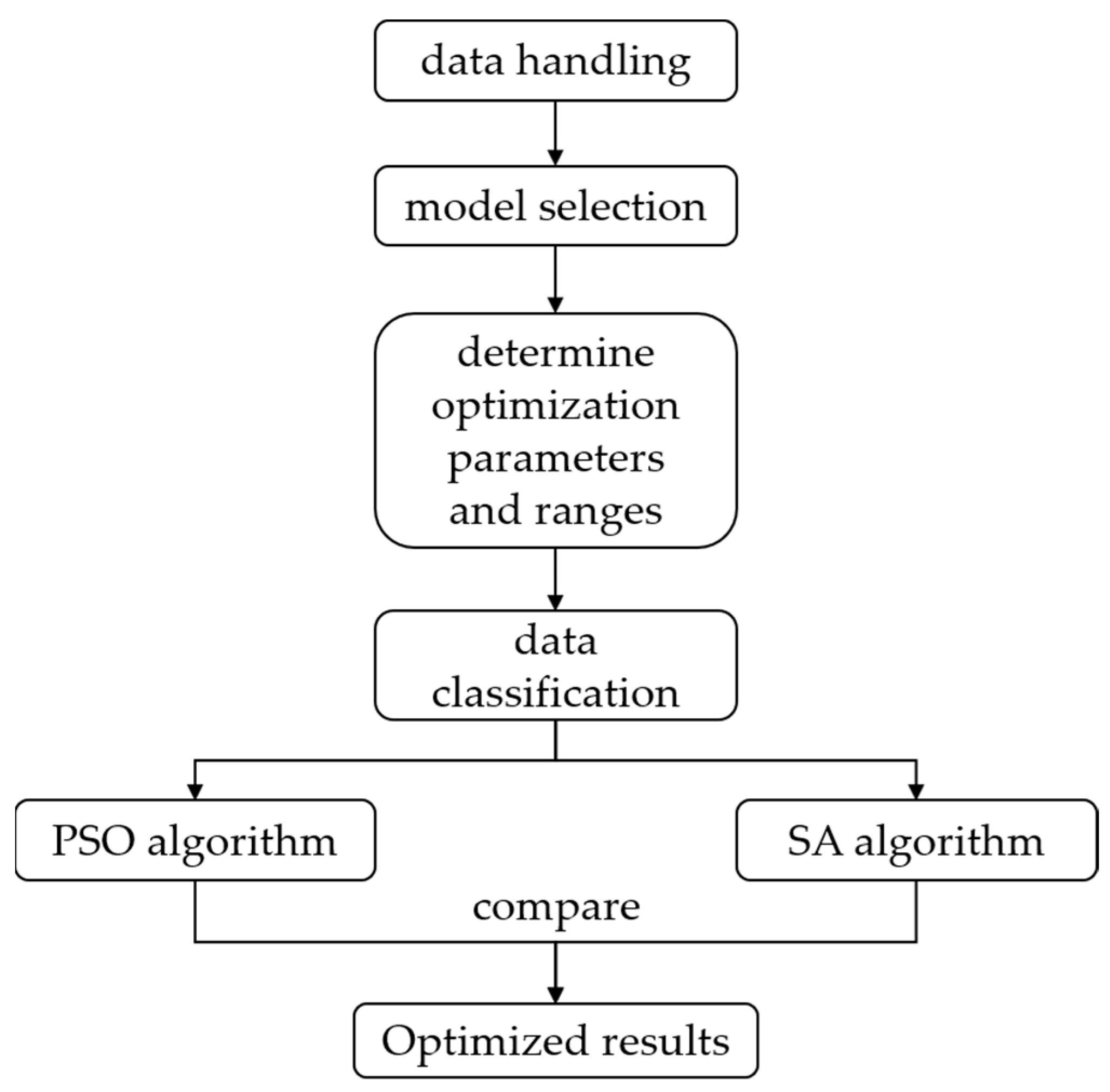
The optimization process of the evaporation duct prediction model, driven by optimization algorithms, comprises four key steps. The first step is data handling. The second step involves model selection followed by the third step where we determine the parameters to be optimized and their respective ranges. Lastly, the fourth step encompasses data classification and model optimization. The specific process is shown in Figure 1.
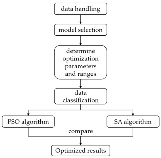
Figure 1.
The flowchart.
The main details are described further. First, the collected meteorological and hydrological data need to be quality controlled, for example, by using the sliding average method to eliminate the noise problems present in the data. The required data are organized into the form of datasets to be passed into the evaporation duct prediction model.
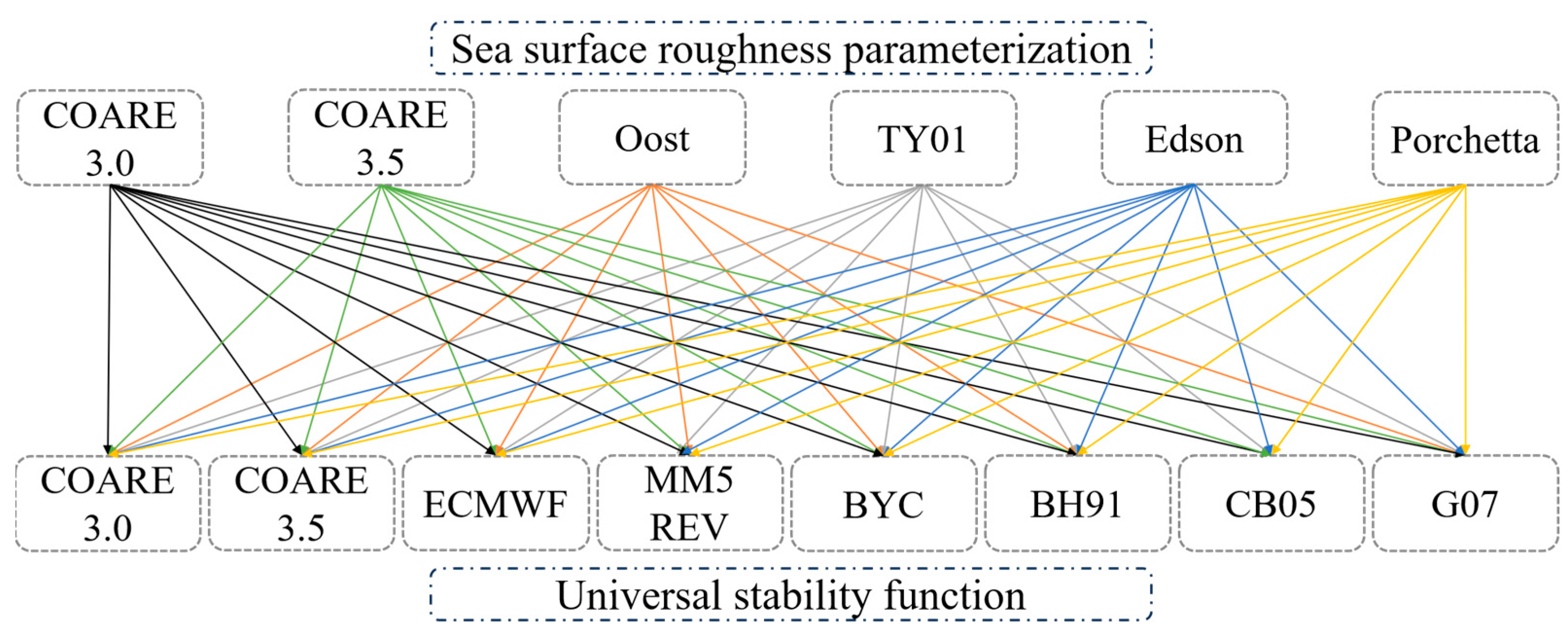
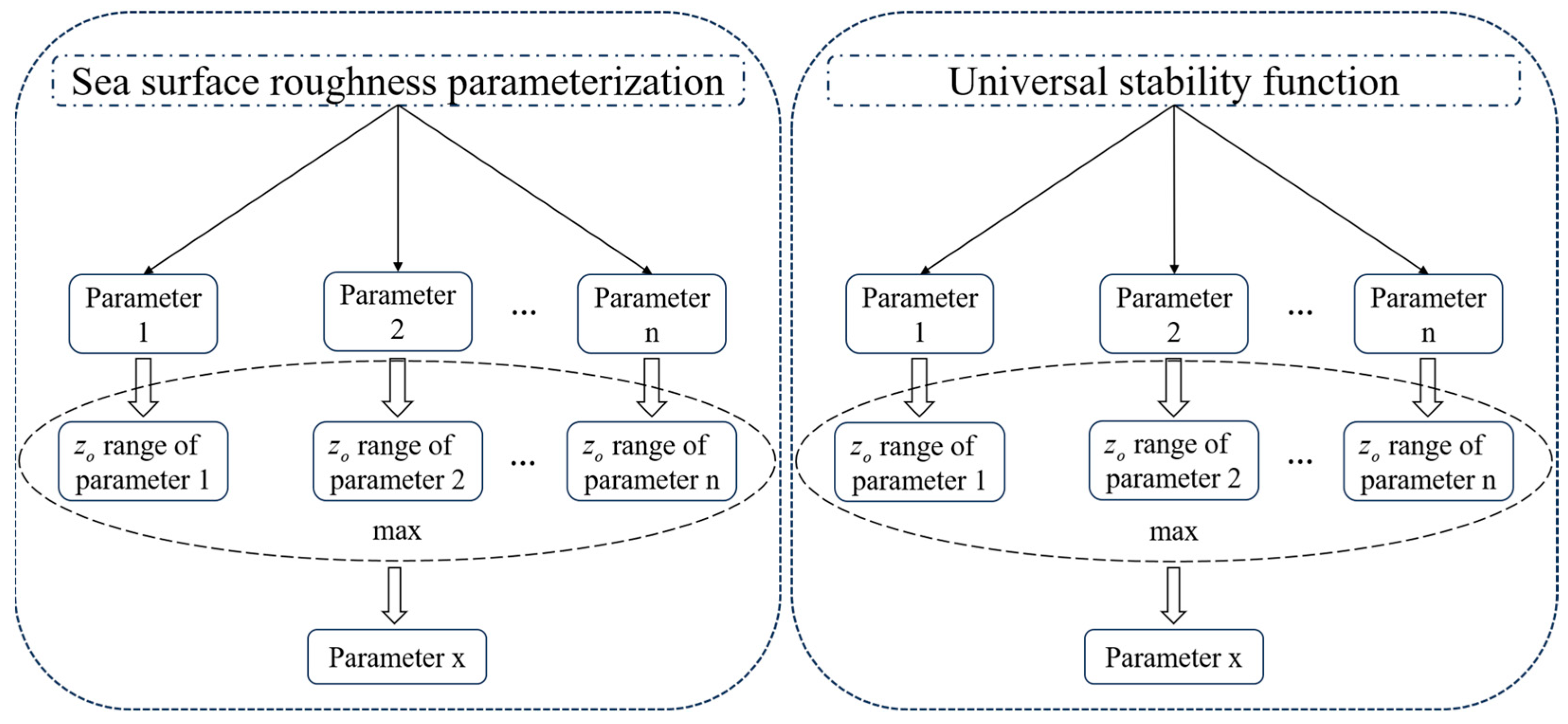
Second, in order to enhance optimization efficiency, we need to choose the combination model of the sea surface roughness parameterization scheme and the universal stability function under the original parameter conditions, thereby obtaining the combination model with the best prediction accuracy in the specific sea area. Figure 2 is model combination.
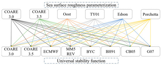
Figure 2.
Model combination.
rms is the root mean square deviation of the value between and , which is used to be the fitness of the accuracy of the model prediction results. is the modified refractivity profile of the model output, is the modified refractivity profile by environmentally measured. The smaller the deviation, , the higher the model prediction accuracy:
where i denotes the order of the measurement level, I is the total number of measurement levels, j is the sequence of the sample and J signifies the total sample count. For the jth sample at the ith layer, is the observed modified refractivity and is the corresponding predicted value from the model.
Third, after obtaining the optimal combination of models, we need to determine the parameters of the sea surface roughness parameterization scheme (e.g., a, b in TY01) and the parameters of the universal stability function (e.g., , in in the stable condition of G07) and the optimization ranges of the corresponding parameters. If the function comprises multiple coefficients, we select some parameters of this function to ensure an equal number of coefficients to be optimized for each function given in Figure 3.
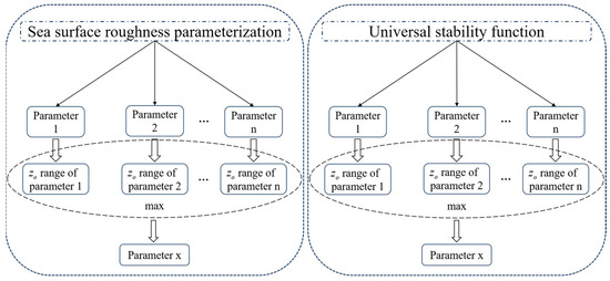
Figure 3.
Parameter selection.
If the function contains multiple parameters, it is necessary to select from these parameters. In the premise of the same variation range for each parameter, we select the parameters that are the most influential to and values, take them as the optimization parameters through observing the changes range in and by adjusting the parameter values. It should be noted that we need to ensure that the number of parameters to be optimized in both functions is the same when exploring the impact of sea surface roughness parameterization schemes and universal stability functions on prediction results. Subsequently, we use the method of exhaustive search to determine the range of parameters to be optimized under the condition that the function’s variation trend does not undergo abrupt changes.
Finally, we divide the dataset into stable and unstable condition samples by using Equation (1) and separately optimize both types of the two samples. The sea surface roughness parameterization selected in step two and the original parameters for universal stability functions are used as initial values for the PSO and SA algorithm. The parameter range to be optimized is set as the upper and lower bounds for the optimization algorithm. Parameters are optimized based on fitness Functions (29) and (30) and iterative iterations are performed to obtain the parameter values corresponding to the minimum fitness value. Unlike the fitness function in step one, since may have measurement errors at different heights, we use the fitted and modified refractivity as the reference value. By comparing and analyzing the accuracy optimization of the refractivity profiles with the two optimization algorithms, the optimization algorithm with the best optimization results is selected to improve the accuracy of predicting refractivity profiles in the specific sea area.
4. Experiment
4.1. Shipboard Data Acquisition Experiment
The research of the evaporation duct prediction model relies on observation data. Many studies have set up meteorological gradient towers near the coast to collect the necessary meteorological and hydrological data. However, this method can only collect data at a single location and the sensor measurement accuracy is not high. These data cannot represent the spatiotemporal characteristics of the specific sea area. High-precision meteorological and hydrological observations near the sea surface are crucial for optimizing the evaporation duct prediction model. Due to the lack of high-precision meteorological and hydrological observation data in the specific sea area, this study installed high-precision meteorological and hydrological sensors at five different heights above the sea surface on the research vessel “Xiangyanghong 18” and conducted a 23-day observation of meteorological and hydrological data near the sea surface. High-precision observation data of wind speed, atmospheric temperature, atmospheric humidity, sea surface skin temperature, atmospheric pressure and other parameters were obtained under different spatiotemporal conditions.
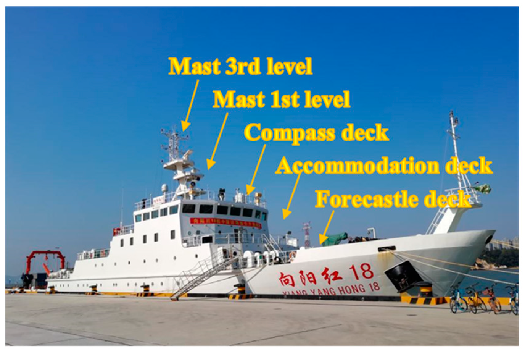
To reduce the impact on the measurement accuracy of sensors, it is necessary to ensure that the installation locations of sensors are as open and unobstructed as possible. As shown in Figure 4, high-precision Humidity and Temperature sensors are installed at the Forecastle deck (6 m), Accommodation deck (8.3 m), Compass deck (13.1 m), Mast 1st floor (14.8 m) and Mast 3rd floor (22.3 m) to achieve layered measurements of atmospheric temperature and humidity at different heights near the sea surface. Barometers, Weather stations and Infrared thermometers are installed on the Compass deck to respectively obtain observation data for atmospheric pressure, wind speed and sea surface skin temperature. The sensor locations as shown in Figure 4. The specifications of the sensors as shown in Table 1. All high-precision observation data are sent to the data collector at the ship’s data center. In this paper, we optimize the evaporation duct forecasting model by using meteorological and hydrological observation data that were collected by the research vessel “Xiangyanghong 18” from 1 April to 23 April, as shown in the cruise route map in Figure 5 (cruise number NORC2021-02-1).

Figure 4.
Sensor locations on R/V.

Table 1.
Sensor specification and installation locations.
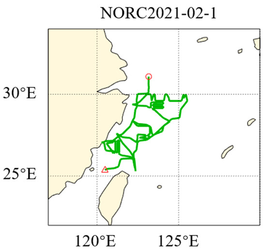
Figure 5.
Cruise trajectories, “Δ” marks the start point and “◯” marks the end point.
4.2. Shipboard Data
The meteorological hydrological sensor used in this study has a data sampling frequency of 1 Hz. A total of 1,987,200 data points were collected from 1 April 2021, 00:00:00 to 23 April 2021, 23:59:59 at the second-level resolution. Before inputting the collected observation data into the evaporation duct prediction model, it is necessary to perform a moving average on the instantaneous observation data to eliminate sensor incidental variations and noise data in the dataset (such as spikes and missing values); thus, we can obtain the observation data that represent the environmental characteristics of the sea area. In this study, a 10 min sliding average window was used for data preprocessing. For true wind observation data, it was first decomposed into north wind and east wind components, then subjected to sliding averaging and synthesis to obtain the required average wind speed and wind direction data. The processed hourly data at whole-hour timestamps were selected as the dataset for further analysis, totaling 552 data points (from 1 April 2021, 00:00:00 to 23 April 2021, 23:00:00).
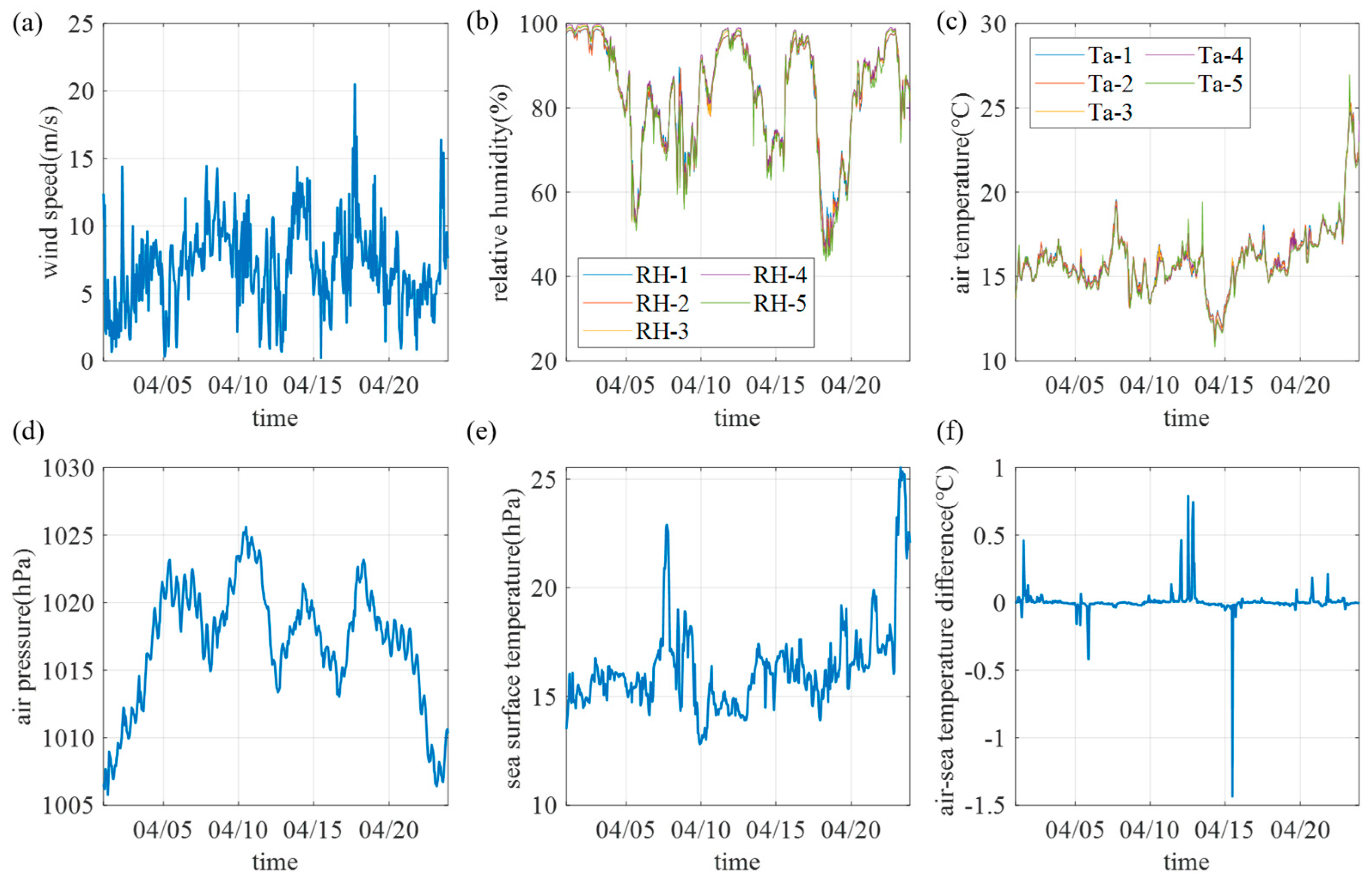
Figure 6 shows the temporal distribution of data after processing for NORC2021-02-1 cruise. Figure 6a represents the wind speed (u) data. Most of the time, the wind speed varies between 0 to 15 m/s, with occasional variations reaching up to 21 m/s. Figure 6b presents relative humidity (RH) data collected at five different heights above the sea surface, namely RH-1, RH-2, RH-3, RH-4 and RH-5 at 6 m, 8.3 m, 13.1 m, 14.8 m and 22.3 m heights, respectively. The RH values range from 43% to 100%, with the majority of the time having RH values above 60%. Figure 6c shows air temperature () data collected at the same five heights as RH. The five curves represent temperature variations at different heights, ranging from 10 °C to 27 °C. Except for 23 April, the temperature data are mostly below 20 °C. Figure 6d displays atmospheric pressure (P) data, which range from 1006 hPa to 1026 hPa. Figure 6e exhibits sea surface temperature () data, with a range of 12 °C to 26 °C. Finally, Figure 6f presents the Richardson number (), calculated by the collected data, which indicates atmospheric stability. According to the statistical results of the data, out of 552 hourly samples collected during the NORC2021-02-1 cruise, there are 273 samples when the atmosphere is in a stable condition and 279 samples when it is in an unstable condition, with more samples indicating an unstable atmosphere.
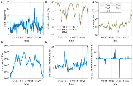
Figure 6.
NORC2021−02−1 data, (a) is the wind speed, (b) is the relative humidity, (c) is the air temperature, (d) is the atmospheric pressure, (e) is sea surface temperature, (f) is the Richardson number.
From Section 2.2, it can be seen that different sea surface roughness parameterization schemes employ various methods to derive sea surface roughness. Some sea surface roughness parameterization schemes (such as Oost, TY01, Porchetta, Edson) utilize wave data, such as significant wave height, wave period, wave direction, etc., to calculate sea surface roughness. In this study, since the shared research cruise did not include sensors for collecting wave data, to ensure data quality, the necessary wave data were obtained from ERA5 reanalysis data [38].
For layered observations of temperature and humidity, least squares fitting was used to derive the referenced modified refractivity profile in each time instant to act as baselines in the following optimization procedures.
where z is the height from the sea surface, i denotes the order of the measurement level, j is the sample serial number and , , are the fitting coefficients. To eliminate the refractivity noise at different heights in the subsequent optimization, the least-squares fitting process was constrained to ensure that the modified refractivity calculated by the model at the height of the ith layer is the same as the modified refractivity value measured at the corresponding layer.
4.3. Evaporation Duct Prediction Model Selection
In accordance with Step 2 in Section 3.4, the model is selected. The sea surface roughness parameterization scheme from Section 2.2 is combined with the universal stability function from Section 2.3 to obtain a new evaporation duct prediction model. The performance of the combined model is evaluated using the NORC2021-02-1 high-precise observation dataset, with Equation (32) as the evaluation criterion. The combined model with the highest prediction accuracy is selected as the model for optimization.
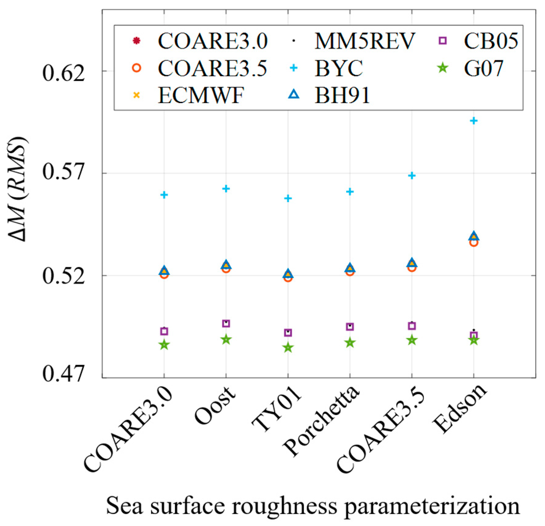
As shown in Figure 7, when using the same universal stability function with different sea surface roughness parameterization schemes, the combination model using the BYC universal stability function has the largest difference in the predicting rms, with an rms difference of 0.0379. The combination model using the G07 universal stability function has the smallest difference in the predicting rms, with an rms difference of 0.004. When using the same sea surface roughness parameterization scheme with different universal stability function combinations, the combination model using the Edson sea surface roughness parameterization scheme has the largest difference in predicting rms, with an rms difference of 0.1072, while the combination model using the TY01 sea surface roughness parameterization scheme has the smallest difference in predicting rms, with an rms difference of 0.073. From the above data, it can be seen that the universal stability function has a greater impact on the model’s prediction results than the sea surface roughness parameterization scheme. Among the 48 predicted models for evaporation duct, the combination model using the TY01 sea surface roughness parameterization scheme and the G07 universal stability function in the specific sea area has the highest accuracy, with an rms of 0.4848. Therefore, the combination model using the TY01 sea surface roughness parameterization scheme and the G07 universal stability function is selected as the model to be optimized.
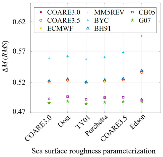
Figure 7.
Comparison of Evaporation duct Prediction Models.
4.4. Parameters to Be Optimized
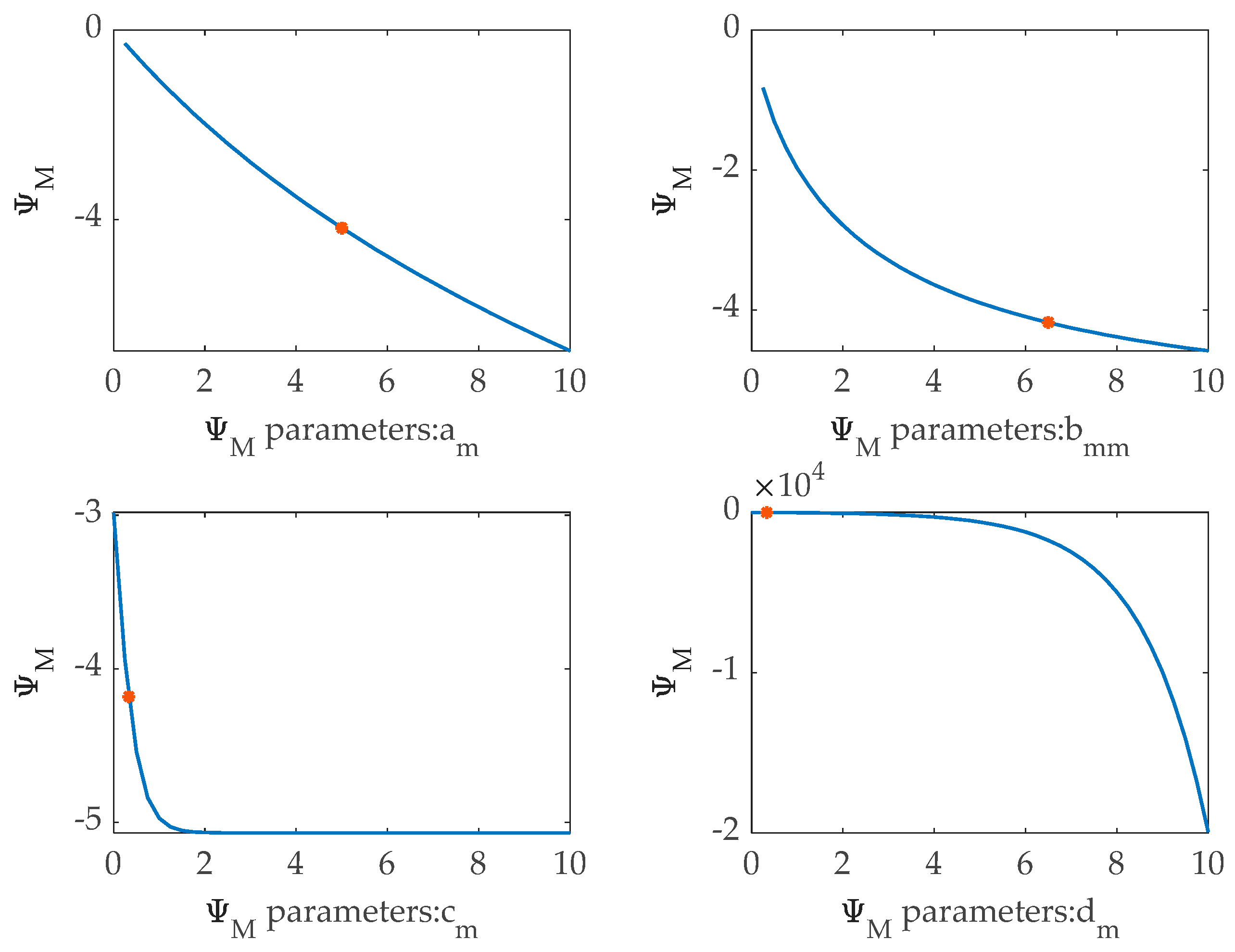
In accordance with Step 3 in Section 3.4, we determine the coefficients to be optimized and their respective ranges. For the selected sea surface roughness parameterization of TY01 and the universal stability function of G07, only variables and contain more than two parameters. To ensure that the number of parameters to be optimized in each function is consistent, it is necessary to select parameters contained in and . Parameter range [0, 10] is used while keeping the other parameters unchanged. Figure 8 and Figure 9 illustrate the influence of various parameters on the values of and .
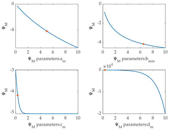
Figure 8.
The effect of different parameters on . “*” is original , “−” is optimized .
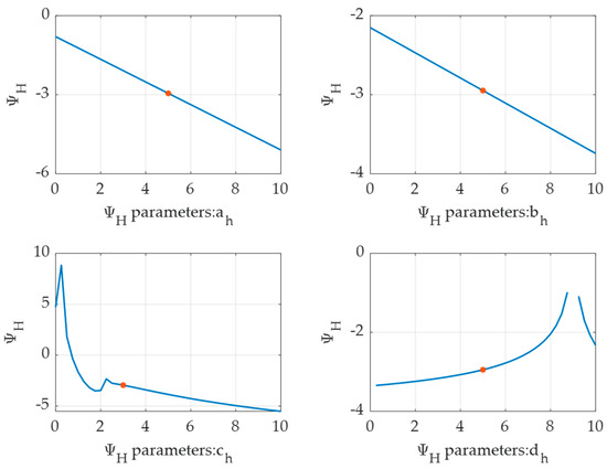
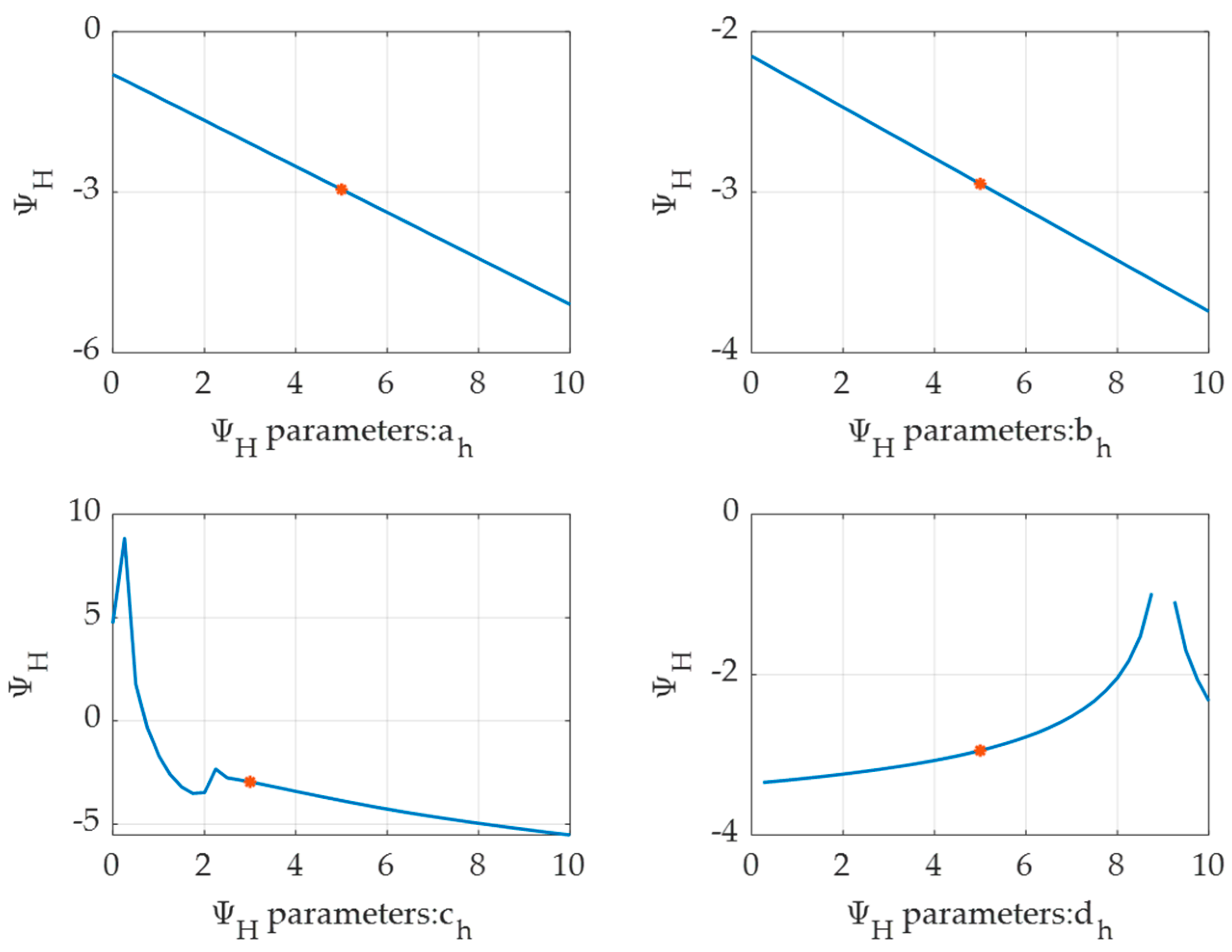
Figure 9.
The effect of different parameters on . “*” is original , “−” is optimized .
From Figure 8 and Figure 9, it is evident that among the four parameters of , the change in the value of has the greatest effect on the value of , followed by the effect of , for a consistent range of parameter variations. Among the four parameters of , the change in has the greatest influence on the value of , and the influence of is the second largest. Therefore, and are selected as parameters to be optimized, and are parameters to be optimized.
While ensuring the continuity and monotonicity of the function, the method of enumeration is used to select the range of changes for each parameter. Table 2 lists the optimized parameters and their optimization ranges for the TY01 sea surface roughness parameterization scheme and the G07 universal stability function.
Table 2.
Parameters to optimize and corresponding numeric range.
4.5. Optimization Results
In accordance with Step 4 in Section 3.4, we divide the observation data into samples corresponding to stable or unstable condition, taking Equation (1) as the criterion for determining atmospheric condition. This division is performed to optimize different functions of the model under different atmospheric conditions in subsequent steps. The TY01 sea surface roughness parameterization scheme and the original parameter values of the G07 universal stability function are used as the initial values for the optimization functions, with the range of optimization parameters set as the upper and lower bounds. The particle swarm optimization algorithm and the simulated annealing algorithm are employed to reference and adjust the refractivity profile , the model output modified refractivity profile , based on the root mean square deviation as the fitness evaluation criterion. After 20 experiments, the parameter values corresponding to the minimum fitness value are determined. The optimization results are presented in Table 3.
Table 3.
NORC2021-02-1 optimization results.
From Table 3, it can be seen that when the number of iterations is the same, both optimization algorithms can approximate the optimal value when optimizing a single function. However, when optimizing multiple functions simultaneously, PSO uses more computational resources because it is a population-based algorithm. Therefore, compared to the SA algorithm, the PSO algorithm is easier to approximate the solution of global optimum.
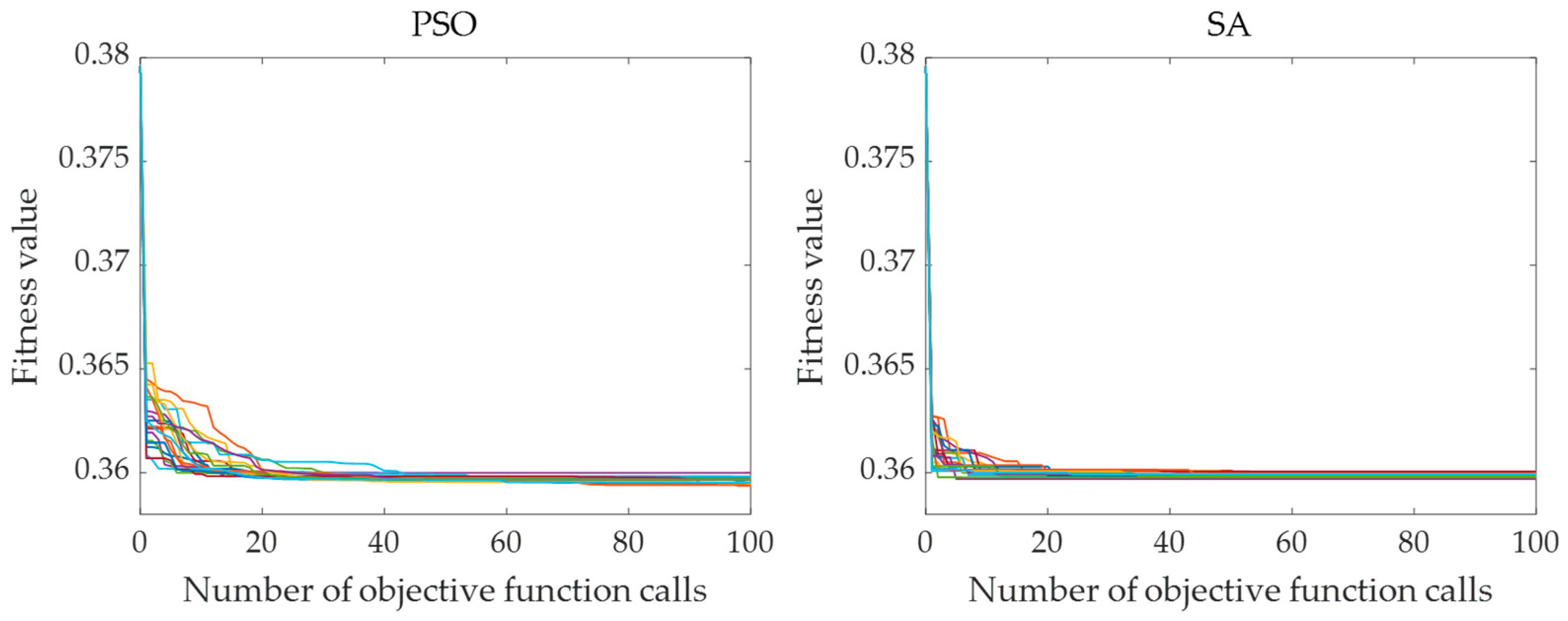
From Figure 10, we can see that both optimization algorithms converge within 100 iterations, and the particle swarm optimization algorithm converges better than the simulated annealing algorithm overall. The average value of the optimal fitness of the particle swarm optimization algorithm for 20 experiments is 0.3596, and its average running time is 4173.2 s. The average value of the optimal fitness of the simulated annealing algorithm for 20 experiments is 0.3599, and its average running time is 4829.7 s. From this, we can conclude that optimization algorithms can be applied to improve the accuracy of predicting the modified refractivity profile. Among them, the PSO algorithm is more effective in improving the accuracy of predicting the modified refractivity profile results.

Figure 10.
Convergence of PSO algorithm and SA algorithm.
When using the above two optimization algorithms to optimize model parameters, the optimization results of samples under unstable conditions are better than those under stable conditions. This result confirms the applicability issues of sea surface roughness parameterization schemes and universal stability functions in the specific sea area. From the optimization results, optimizing parameter has the best effect on improving the accuracy of modified refractivity profile predictions, followed by optimizing parameter . The impact of optimizing sea surface roughness parameters and on the accuracy of modified refractivity profile predictions is relatively small. This conclusion is consistent with Section 3.4; namely, in the specific sea areas, the universal stability function has a greater impact on the accuracy of modified refractivity profile predictions than the sea surface roughness parameterization scheme. Since optimizing parameter has a significantly better effect on improving the accuracy of modified refractivity profile predictions than optimizing other parameters, combination optimization including is superior to combination optimization that only includes and .
5. Summary
We propose a method to improve the accuracy of the prediction model of evaporation duct by using optimization algorithms in this paper. Firstly, high-precise meteorological and hydrological observation data in different heights at the sea surface are collected by installing sensors on a shipborne platform. Wave data are obtained from ERA5 reanalysis data. A least-squares fit is applied to the measured near-sea-surface refractivity profiles based on a fitting formula, resulting in a reference modified refractivity profile near the sea surface. Data collection is used to select sea surface roughness parameterization and universal stability function, yielding a more accurate evaporation duct prediction model for the specific sea area, which is the model to be optimized. The coefficients of the model are determined and coefficient selection is performed for functions with multiple coefficients, ensuring that the number of coefficients to be optimized in each function is the same, the range of values for the coefficients to be optimized is determined.
We use PSO and SA algorithms to optimize the sea surface roughness parameterization and the coefficients of the universal stability function. Comparing with the model’s performance before optimization, under stable conditions, the accuracy of NORC2021-02-1 cruise prediction improved by 5.09% and 4.75% when using the PSO and SA algorithms. Under unstable conditions, the prediction accuracy increased by 9.97% with the PSO algorithm and 9.89% with the SA algorithm. These results confirm the feasibility of applying optimization algorithms to improve the accuracy of modified refractivity profile predictions. Using the PSO algorithm is more effective in enhancing the accuracy of modified refractivity profile predictions, indicating that the model optimized with the particle swarm optimization algorithm has better applicability in certain sea areas and seasons. This paper is a preliminary attempt to improve the accuracy of modified refractivity prediction using optimization algorithms, so the classical PSO algorithm and the SA algorithm are used. In subsequent studies, the accuracy of modified reflectivity prediction will be improved by using other optimization algorithms or improved variants of optimization algorithms, such as the differential evolution method, as well as Grew Wolf Optimization [39,40], Biogeography Based Optimization [41] and Social Network Optimization [42], which has been shown to outperform particle swarm algorithms and has been applied to parameter identification.
6. Discussion
The Monin–Obukhov similarity theory [15] pointed out that is a continuous and monotonous function, with . In this study, without altering the form of and its underlying physical laws, model parameters are optimized. Experimental results have confirmed the feasibility of applying the optimization algorithm to the study of evaporation duct prediction models. Most existing research on evaporation duct assumes that the function is a monotonous function, but there is still not clear consensus on whether the function in nature is a monotonous function. In the following research, the continuity of the function will be a key focus.
In addition to obtaining more accurate evaporation duct parameters (such as modified refractivity and evaporation duct height) based on the Monin–Obukhov similarity theory, some studies have utilized machine learning algorithms, such as BP neural networks and LS-SVM, to directly predict the evaporation duct height using known meteorological and hydrological data. While this approach does not adhere to the Monin–Obukhov similarity theory, it can also lead to improved accuracy in predicting the evaporation duct height. We present a statistical analysis of the mean variation of the optimized model’s evaporation duct height in this paper.
Because , and have a minimal impact on the accuracy of the model’s predictions, it is not necessary to optimize their coefficients separately. As can be seen from Table 4, the improvement percentage of the evaporation duct height is not a simple linear relationship with the predicted accuracy of the modified refractivity. For example, when optimizing all coefficients, using the particle swarm optimization algorithm yields better results for optimizing the modified refractivity than using the simulated annealing algorithm, but the optimization effect for the evaporation duct height is the opposite. Under unstable conditions of the modified refractivity, the optimization effect is better than under stable conditions, but the optimization effect for the evaporation duct height is similarly opposite.
Table 4.
NORC2021-02-1 evaporation duct height optimization results.
To investigate which parameter of the evaporation duct, either the height or the modified refractivity profile, is more suitable as the accuracy criterion for predicting the evaporation duct prediction model, two groups of samples were selected to observe the propagation path loss of electromagnetic waves. The first group of samples consists of profiles with significant differences in modified refractivity profiles but relatively small differences in evaporation duct heights. The second group of samples consists of profiles with relatively small differences in modified refractivity profiles but significant differences in evaporation duct heights. The parameters set for electromagnetic wave propagation in the sea surface are as follows: the maximum range of electromagnetic wave propagation is set to 150 km, the maximum altitude is set to 100 m, of which the range step is 200 m, the altitude step is 0.1 m, the 3 dB beamwidth is 1 deg, the frequency is 3000 MHz, the dielectric constant is 69.134 and the conductivity is 7.1462 s/m.
The first group of samples shows the height of the evaporation duct and the modified refractivity profile as shown in Figure 11. The antenna height is set to 13 m, which means the antenna is located outside the evaporation duct. We calculate the path loss generated by the two profile sets.
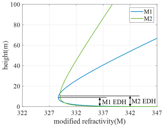
Figure 11.
Group 1: EDH and modified refractivity.
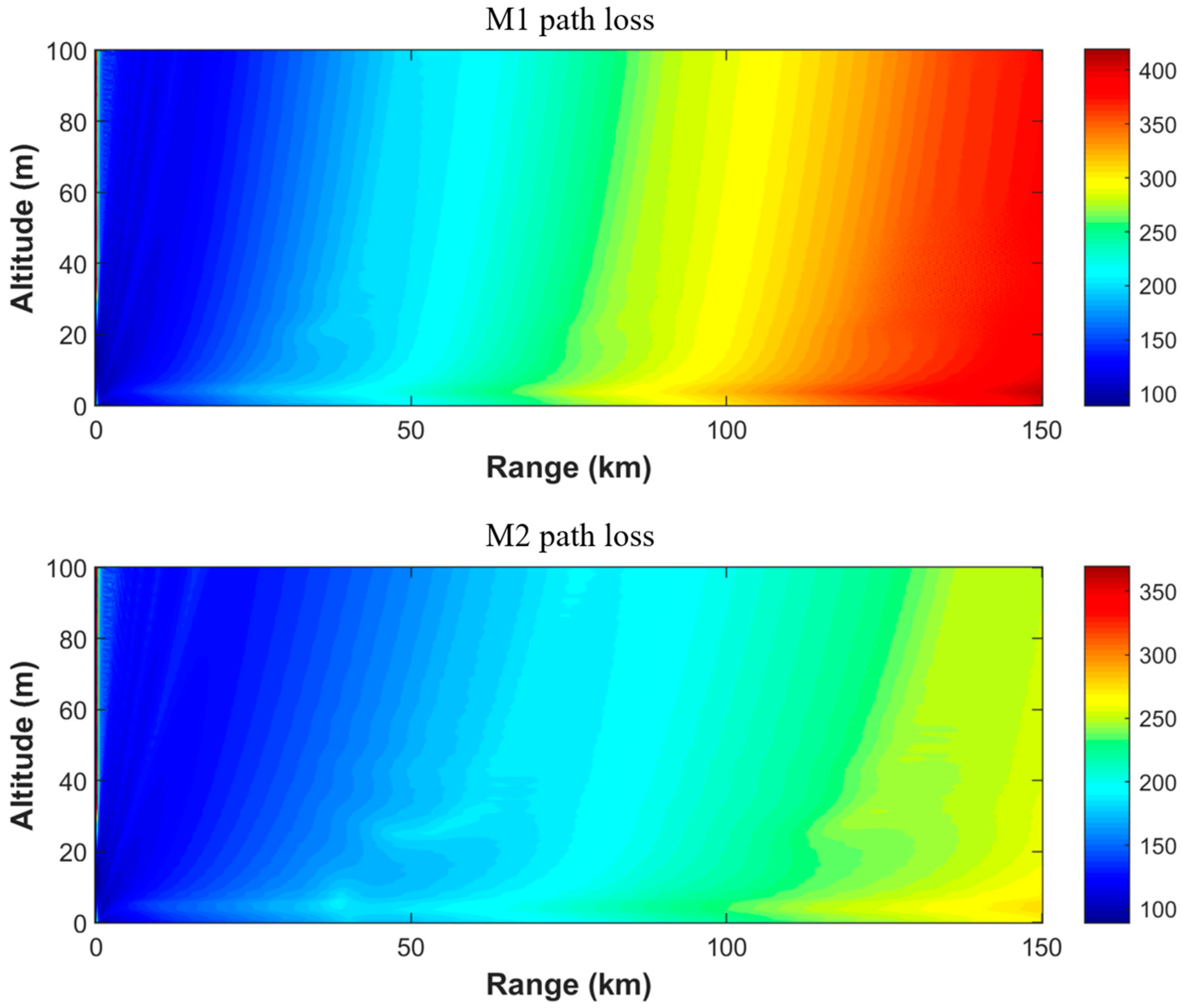
From Figure 12, it can be seen that the path loss is directly proportional to the propagation distance. Within a distance of 0–50 km, the path losses for the M1 and M2 profiles are similar, with no significant differences. However, in the range of 50–100 km, there is a noticeable difference in path loss between the two, with the path loss for the M2 profile significantly lower than that of M1. When the distance exceeds 100 km, the difference in path loss between the two profile groups further increases, with the path loss for M2 profile much lower than that of M1 profile. As shown in the above figure, even when the evaporation duct height is similar, the electromagnetic wave path loss exhibits significant differences due to different refractivity profile corrections.

Figure 12.
First group path loss.
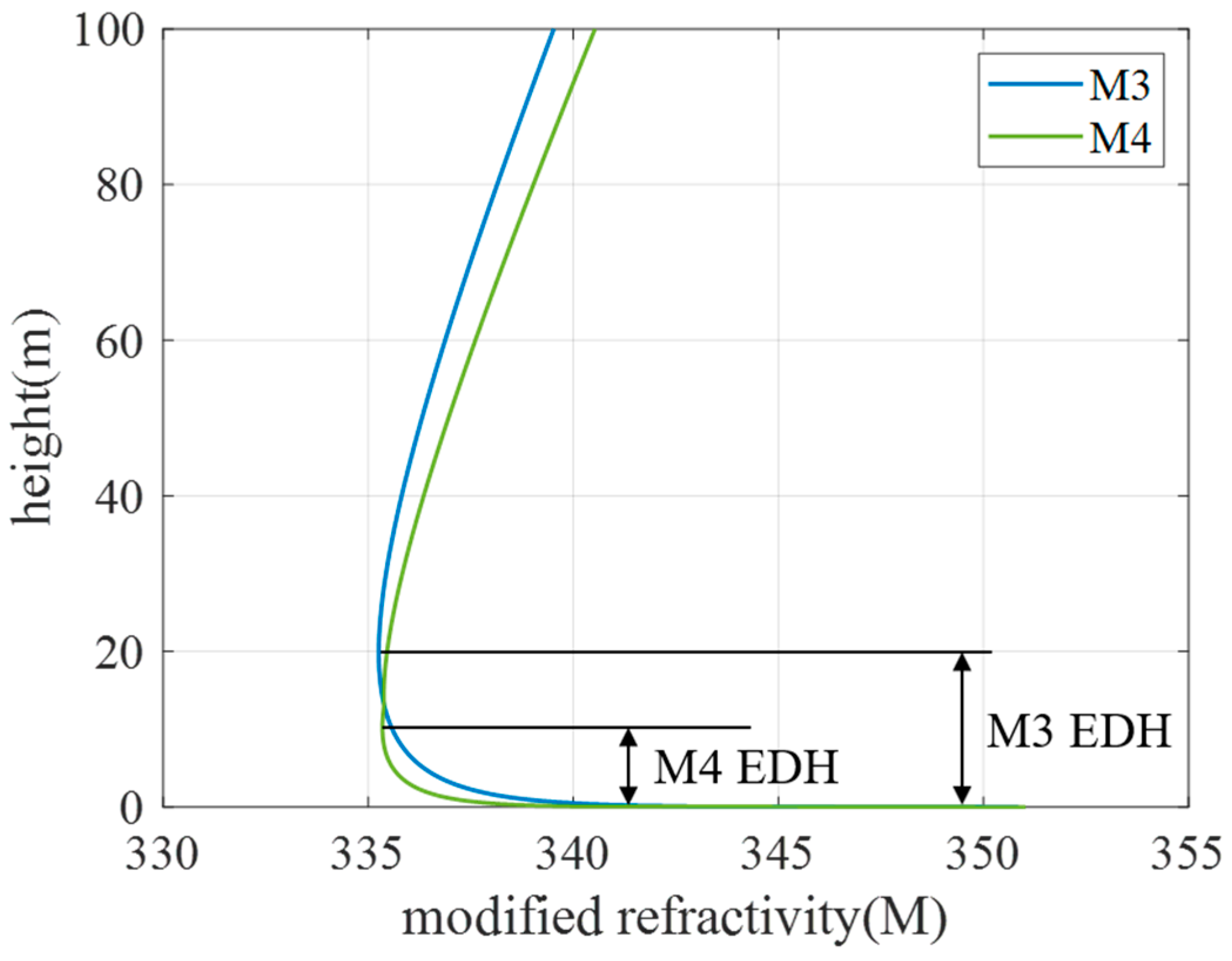
The second group of sample evaporation duct height and modified refractivity profiles is shown in Figure 13. The antenna height is 22 m. The path loss resulting from the two sets of profiles is calculated.
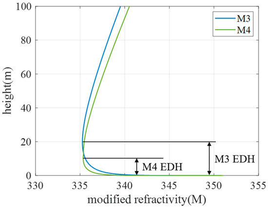
Figure 13.
Group 2: EDH and modified refractivity.
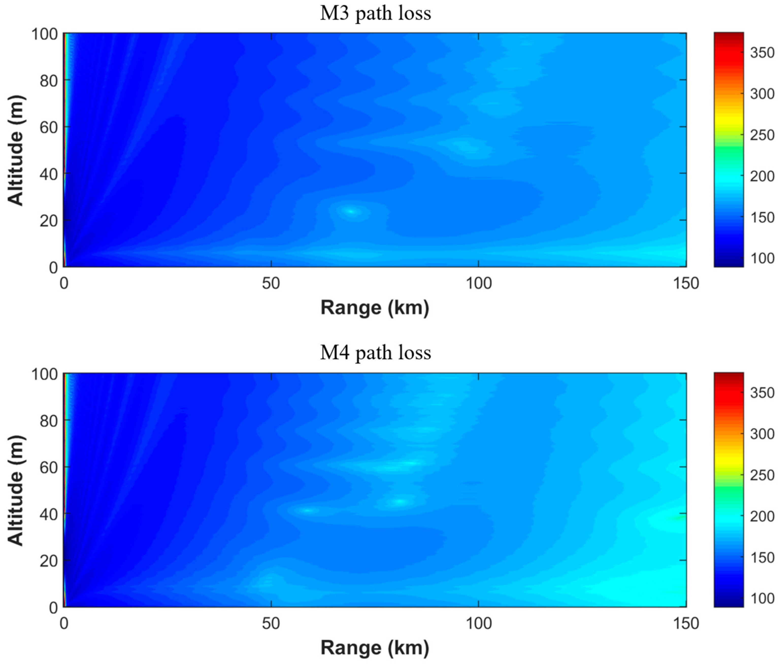
From Figure 14, it can be seen that within a distance of 0–50 km, the path loss difference between profiles M3 and M4 is very small. When the distance exceeds 50 km, the path loss of profile M4 is higher than that of profile M3, but the loss difference is significantly smaller than the first group of profiles. The differences in refractivity profiles are small, even when there is a significant difference in evaporation duct height, the electromagnetic wave path loss does not have too much variation.

Figure 14.
Second group path loss.
From the above information, it can be seen that path loss is directly proportional to propagation distance, the influence of evaporation duct height on path loss is much smaller than the influence of the modified refractivity profile on path loss. In other words, the difference in path loss of electromagnetic waves mainly originates from different modified refractivity profiles. In order to obtain a predictive model for evaporation duct with higher accuracy, the modified refractivity profile is a physical quantity that must be considered and it is more suitable as a standard for evaluating the predictive accuracy of the evaporation duct prediction model. Subsequent research should focus on the modified refractivity profile to achieve high-precision prediction of evaporation duct based on predicting the modified refractivity profile.
Author Contributions
Conceptualization, Y.C.; methodology, Y.C.; software, Y.C.; validation, Y.C.; formal analysis, Y.C.; investigation, Y.C.; data curation, Y.C.; writing—original draft preparation, Y.C.; writing—review and editing, Y.C.; supervision, T.H., Z.Q., J.Z., Z.L., B.W. and K.Q. All authors have read and agreed to the published version of the manuscript.
Funding
The National Natural Science Foundation of China (Grant Nos. 42176185, 42206188 and 42076195); the Natural Science Foundation of Shandong Province of China (Grant Nos. ZR2021MD114, ZR2020QD085 and ZR2020MF022); the Key Research and Development Program of Shandong Province of China (Grant No. 2023CXPT015).
Data Availability Statement
Data can be obtained upon request from the corresponding author of this article.
Acknowledgments
Shipborne data acquisition was supported by the National Natural Science Foundation of China Open Research Cruise (No. NORC2021-02+NORC2021-301), which is funded by the Shiptime Sharing Project of the National Natural Science Foundation of China. This cruise was conducted on board the R/V Xiangyanghong 18 by the First Institute of Oceanography, Ministry of Natural Resources, China.
Conflicts of Interest
The authors declare no conflict of interest.
References
- Xu, L.; Yardim, C.; Haack, T. Evaluation of COAMPS Boundary Layer Refractivity Forecast Accuracy for 2–40 GHz Electromagnetic Wave Propagation. Radio Sci. 2022, 57, e2021RS007404. [Google Scholar] [CrossRef]
- Yang, C.; Shi, Y.; Wang, J.; Feng, F. Regional Spatiotemporal Statistical Database of Evaporation Ducts Over the South China Sea for Future Long-Range Radio Application. IEEE J. Sel. Top. Appl. Earth Obs. Remote Sens. 2022, 15, 6432–6444. [Google Scholar] [CrossRef]
- Jiang, H.; Li, J. Location privacy-preserving mechanisms in location-based services: A comprehensive survey. ACM Comput. Surv. CSUR 2021, 54, 1–36. [Google Scholar] [CrossRef]
- Ding, J.; Fei, J.; Huang, X.; Cheng, X.; Hu, X.; Ji, L. Development and Validation of an Evaporation Duct Model. Part I: Model Establishment and Sensitivity Experiments. J. Meteorol. Res. 2015, 29, 467–481. [Google Scholar] [CrossRef]
- Yang, S.; Li, X.; Wu, C.; He, X.; Zhong, Y. Application of the PJ and NPS Evaporation Duct Models over the South China Sea (SCS) in Winter. PLoS ONE 2017, 12, e0172284. [Google Scholar] [CrossRef] [PubMed]
- Chai, X.; Li, J.; Zhao, J.; Wang, W.; Zhao, X. LGB-PHY: An Evaporation Duct Height Prediction Model Based on Physically Constrained LightGBM Algorithm. Remote Sens. 2022, 14, 3448. [Google Scholar] [CrossRef]
- Shi, Y.; Yang, K.; Yang, Y.; Ma, Y. A New Evaporation Duct Climatology over the South China Sea. J. Meteorol. Res. 2015, 29, 764–778. [Google Scholar] [CrossRef]
- Zhang, Q.; Yang, K.; Shi, Y. Spatial and Temporal Variability of the Evaporation Duct in the Gulf of Aden. Tellus A Dyn. Meteorol. Oceanogr. 2016, 68, 29792. [Google Scholar] [CrossRef]
- Hong, F.; Zhang, Q. Time Series Analysis of Evaporation Duct Height over South China Sea: A Stochastic Modeling Approach. Atmosphere 2021, 12, 1663. [Google Scholar] [CrossRef]
- Jiang, Y.; Yao, X.; Zhang, Y. An Evaporation Duct Height Estimation Algorithm Based on Deep Neural Networks. J. Phys. Conf. Ser. 2022, 2224, 012020. [Google Scholar] [CrossRef]
- DeMott, C.A.; Klingaman, N.P. Atmosphere-ocean coupled processes in the Madden-Julian oscillation. Rev. Geophys. 2015, 53, 1099–1154. [Google Scholar] [CrossRef]
- Deike, L. Mass transfer at the ocean–atmosphere interface: The role of wave breaking, droplets, and bubbles. Annu. Rev. Fluid Mech. 2022, 54, 191–224. [Google Scholar] [CrossRef]
- Tangang, F.; Chung, J.X. Projected future changes in rainfall in Southeast Asia based on CORDEX–SEA multi-model simulations. Clim. Dyn. 2020, 55, 1247–1267. [Google Scholar] [CrossRef]
- Nadeau, D.F.; Pardyjak, E.R. Similarity scaling over a steep alpine slope. Bound.-Layer Meteorol. 2013, 147, 401–419. [Google Scholar] [CrossRef]
- Grachev, A.A.; Andreas, E.L. The critical Richardson number and limits of applicability of local similarity theory in the stable boundary layer. Bound.-Layer Meteorol. 2013, 147, 51–82. [Google Scholar] [CrossRef]
- Woolway, R.I.; Maberly, S.C. Climate velocity in inland standing waters. Nat. Clim. Chang. 2020, 10, 1124–1129. [Google Scholar] [CrossRef]
- Jiménez, P.A.; Dudhia, J.; González-Rouco, J.F.; Navarro, J.; Montávez, J.P.; García-Bustamante, E. A Revised Scheme for the WRF Surface Layer Formulation. Mon. Weather Rev. 2012, 140, 898–918. [Google Scholar] [CrossRef]
- Tian, B.; Liu, Q.; Lu, J.; He, X.; Zeng, G.; Teng, L. The Influence of Seasonal and Nonreciprocal Evaporation Duct on Electromagnetic Wave Propagation in the Gulf of Aden. Results Phys. 2020, 18, 103181. [Google Scholar] [CrossRef]
- Frederickson, P.; Alappattu, D.; Wang, Q.; Yardim, C.; Xu, L.; Christman, A.; Fernando, H.J.S.; Blomquist, B. Evaluating the Use of Different Flux-Gradient Functions in NAVSLaM During Two Experiments. In Proceedings of the 2018 IEEE International Symposium on Antennas and Propagation & USNC/URSI National Radio Science Meeting, Boston, MA, USA, 8–13 July 2018; pp. 885–886. [Google Scholar]
- Shami, T.M.; El-Saleh, A.A. Particle swarm optimization: A comprehensive survey. IEEE Access 2022, 10, 10031–10061. [Google Scholar] [CrossRef]
- Hashizume, T.; Ying, B.W. Challenges in developing cell culture media using machine learning. Biotechnol. Adv. 2023, 70, 108293. [Google Scholar] [CrossRef]
- Wang, B.; Wu, Z.-S.; Zhao, Z.; Wang, H.-G. Retrieving Evaporation Duct Heights from Radar Sea Clutter Using Particle Swarm Optimization (PSO) Algorithm. Prog. Electromagn. Res. M 2009, 9, 79–91. [Google Scholar] [CrossRef]
- Wang, Q.H.; Bedoya-Pinto, A. The magnetic genome of two-dimensional van der Waals materials. ACS Nano 2022, 16, 6960–7079. [Google Scholar] [CrossRef] [PubMed]
- Mohseni, N.; McMahon, P.L. Ising machines as hardware solvers of combinatorial optimization problems. Nat. Rev. Phys. 2022, 4, 363–379. [Google Scholar] [CrossRef]
- Tirkolaee, E.B.; Goli, A.; Ghasemi, P. Designing a sustainable closed-loop supply chain network of face masks during the COVID-19 pandemic: Pareto-based algorithms. J. Clean. Prod. 2022, 333, 130056. [Google Scholar] [CrossRef] [PubMed]
- Zhao, X.; Huang, X. Remote Sensing of Atmospheric Duct Parameters Using Simulated Annealing. Chin. Phys. B 2011, 20, 099201. [Google Scholar] [CrossRef]
- De Leeuw, G.; Andreas, E.L. Production flux of sea spray aerosol. Rev. Geophys. 2011, 49. [Google Scholar] [CrossRef]
- Warner, J.C.; Armstrong, B. Development of a coupled ocean–atmosphere–wave–sediment transport (COAWST) modeling system. Ocean. Model. 2010, 35, 230–244. [Google Scholar] [CrossRef]
- Ricchi, A.; Bonaldo, D. Simulation of a flash-flood event over the Adriatic Sea with a high-resolution atmos-phere–ocean–wave coupled system. Sci. Rep. 2021, 11, 9388. [Google Scholar] [CrossRef]
- Edson, J.B.; Jampana, V.; Weller, R.A.; Bigorre, S.P.; Plueddemann, A.J.; Fairall, C.W.; Miller, S.D.; Mahrt, L.; Vickers, D.; Hersbach, H. On the Exchange of Momentum over the Open Ocean. J. Phys. Oceanogr. 2013, 43, 1589–1610. [Google Scholar] [CrossRef]
- Porchetta, S.; Temel, O.; Muñoz-Esparza, D.; Reuder, J.; Monbaliu, J.; van Beeck, J.; van Lipzig, N. A New Roughness Length Parameterization Accounting for Wind–Wave (Mis)Alignment. Atmos. Chem. Phys. 2019, 19, 6681–6700. [Google Scholar] [CrossRef]
- Eriksen, M.; Lebreton, L.C. Plastic pollution in the world’s oceans: More than 5 trillion plastic pieces weighing over 250,000 tons afloat at sea. PLoS ONE 2014, 9, e111913. [Google Scholar] [CrossRef] [PubMed]
- Stevens, R.J.; Meneveau, C. Flow structure and turbulence in wind farms. Annu. Rev. Fluid Mech. 2017, 49, 311–339. [Google Scholar] [CrossRef]
- Fausto, R.S. Programme for Monitoring of the Greenland Ice Sheet (PROMICE) automatic weather station data. Earth Syst. Sci. Data 2021, 13, 3819–3845. [Google Scholar] [CrossRef]
- Sauer, J.A. The FastEddy® resident-GPU accelerated large-eddy simulation framework: Model formulation, dynamical-core validation and performance benchmarks. J. Adv. Model. Earth Syst. 2020, 12, e2020MS002100. [Google Scholar] [CrossRef]
- Zhou, W.; Shen, M.; Zhang, Y.; Wu, D.; Zhu, D. Offshore Surface Evaporation Duct Joint Inversion Algorithm Using Measured Dual-Frequency Sea Clutter. IEEE J. Sel. Top. Appl. Earth Obs. Remote Sens. 2022, 15, 6382–6390. [Google Scholar] [CrossRef]
- Wang, Z.H.; Chang, C.C. Optimizing least-significant-bit substitution using cat swarm optimization strategy. Inf. Sci. 2012, 192, 98–108. [Google Scholar] [CrossRef]
- Bell, M.L.; Catalfamo, C.J. Post-acute sequelae of COVID-19 in a non-hospitalized cohort: Results from the Arizona CoVHORT. PLoS ONE 2021, 16, e0254347. [Google Scholar] [CrossRef]
- Mirjalili, S.; Mirjalili, S.M.; Lewis, A. Grey Wolf Optimizer. Adv. Eng. Softw. 2014, 69, 46–61. [Google Scholar] [CrossRef]
- Emary, E.; Zawbaa, H.M.; Hassanien, A.E. Binary Grey Wolf Optimization Approaches for Feature Selection. Neurocomputing 2016, 172, 371–381. [Google Scholar] [CrossRef]
- Ma, H. An Analysis of the Equilibrium of Migration Models for Biogeography-Based Optimization. Inf. Sci. 2010, 180, 3444–3464. [Google Scholar] [CrossRef]
- Niccolai, A.; Grimaccia, F.; Mussetta, M.; Pirinoli, P.; Bui, V.H.; Zich, R.E. Social Network Optimization for Microwave Circuits Design. Prog. Electromagn. Res. C 2015, 58, 51–60. [Google Scholar] [CrossRef]


Disclaimer/Publisher’s Note: The statements, opinions and data contained in all publications are solely those of the individual author(s) and contributor(s) and not of MDPI and/or the editor(s). MDPI and/or the editor(s) disclaim responsibility for any injury to people or property resulting from any ideas, methods, instructions or products referred to in the content. |
© 2024 by the authors. Licensee MDPI, Basel, Switzerland. This article is an open access article distributed under the terms and conditions of the Creative Commons Attribution (CC BY) license (https://creativecommons.org/licenses/by/4.0/).